A bivariational, stable and convergent hierarchy for time-dependent coupled cluster with adaptive basis sets

Abstract

We propose a new formulation of time-dependent cc with adaptive basis functions and division of the one-particle space into active and secondary subspaces. The formalism is fully bivariational in the sense of a real-valued tdbvp and converges to the complete-active-space solution, a property that is obtained by the use of biorthogonal basis functions. A key and distinguishing feature of the theory is that the active bra and ket functions span the same space by construction. This ensures numerical stability and is achieved by employing a split unitary/non-unitary basis set transformation: The unitary part changes the active space itself, while the non-unitary part transforms the active basis. The formulation covers vibrational as well as electron dynamics. Detailed eom are derived and implemented in the context of vibrational dynamics, and the numerical behavior is studied and compared to related methods.

I INTRODUCTION

Computing the nuclear quantum dynamics of molecules presents a tremendous challenge for systems with more than a few degrees of freedom. One of the most versatile methods that has been developed for this purpose is the mctdh method,Meyer, Manthe, and Cederbaum (1990); Beck et al. (2000) which employs a complete wave function expansion inside an active space spanned by a limited number of adaptive basis functions. The division of the one-particle space into active and secondary parts allows a compact and highly flexible active space, something that is a key factor in the success of the method. An analogous scheme for computing the electron dynamics of molecules is called mctdhf.Zanghellini et al. (2003); Kato and Kono (2004); Nest, Klamroth, and Saalfrank (2005); Caillat et al. (2005) While mctdh and mctdhf constitute important reference approaches in their respective fields, they involve a computational cost that scales exponentially, thus limiting their application to comparatively small systems. It is therefore highly pertinent to investigate and develop alternative methods that are accurate and achieve polynomial scaling, a goal that has motivated an immense amount of research in different directions that we will not attempt to survey here. Instead, we will focus on the cc Ansatz and, specifically, on the idea of combining the time-dependent cc Ansatz with adaptive basis functions. Adaptive or optimized basis functions have a long history in ground-state electronic cc theory, starting with the bcc method,Chiles and Dykstra (1981); Handy et al. (1989); Raghavachari et al. (1990); Hampel, Peterson, and Werner (1992) where the orbitals are determined in such a way that the singles projections vanish. A closely related approach known as occPurvis and Bartlett (1982); Scuseria and Schaefer (1987); Sherrill et al. (1998); Krylov et al. (1998); Pedersen, Koch, and Hättig (1999) instead minimizes the cc energy by using unitary (orthogonal) orbital transformations. It turns out, however, that occ does not reproduce the fci limit,Köhn and Olsen (2005) which is of course a disadvantage. Replacing the unitary (orthogonal) orbital transformation with a non-unitary (non-orthogonal) one defines the nocc method,Pedersen, Fernández, and Koch (2001) which does in fact recover the fci limit, as shown by Myhre.Myhre (2018)

Time-dependent occ and nocc (tdocc and tdnocc) were introduced by Pedersen et al.Pedersen, Koch, and Hättig (1999); Pedersen, Fernández, and Koch (2001) for the purpose of deriving gauge invariant response functions. Concrete working equations for actually propagating the tdocc and tdnocc wave functions in time were, however, not provided. The first example of an explicitly time-dependent cc method with dynamical orbitals is thus Kvaal’s oatdccKvaal (2012) method from 2012, which employs biorthogonal (i.e. non-orthogonal) orbitals. Importantly, this method allows division of the orbital basis and reproduces the mctdhf limit correctly. The oatdcc and tdnocc Ansätze are equivalent if the oatdcc orbital space is not divided into active and secondary parts.

Just as oatdcc can be viewed as a combination of the cc approach with the basic idea of mctdhf, the tdmvccMadsen et al. (2020a) method developed in our group combines vcc with adaptive basis functions in the spirit of mctdh. We have, however, discovered certain stability issues with the tdmvcc approach that occur specifically when the time-dependent biorthogonal basis set is divided.Højlund et al. (2022) Our investigation of the problem showed that it is associated with the following fact: If a biorthogonal basis is divided into active and secondary parts, then there is no guarantee that the active bra functions and the active ket functions span the same space. In itself, this is not necessarily a cause for concern, but we have observed that the two spaces tend to drift dangerously far apart, resulting in serious numerical trouble. In Ref. 21, we proposed a so-called restricted polar version of tdmvcc (rptdmvcc) that forces the active bra and ket spaces to be the same, while allowing non-orthogonality within the active space. The rptdmvcc model was shown to solve the stability issue without compromising accuracy, but it should be stressed that the rptdmvcc equations are not fully bivariational. Apart from being somewhat unappealing from a formal standpoint, this fact also leads to minor energy non-conservation beyond ordinary numerical noise and integration error. Even when energy conservation is not of major interest in itself, it serves as a convenient tool for gauging the integration error (at least for some types of integration schemes) and is therefore a desirable property in practical computations.

A different approach that cannot suffer from the stability issue described above is to simply use an orthogonal basis. Real-time tdocc has indeed been introduced by Sato et al.,Sato et al. (2018) and we have recently considered an orthogonal version of tdmvcc (otdmvcc)Højlund, Zoccante, and Christiansen (2024) analogous to tdocc. Our detailed benchmark calculations confirmed numerically that otdmvcc does not converge to mctdh, which is certainly a disadvantage. In concrete terms, the non-convergence means that one cannot generally expect the quality of oTDMVCC to improve systematically towards the appropriate limit. Although we did not usually observe this deficiency at low excitation levels,Højlund, Zoccante, and Christiansen (2024) it is surely a problem when high accuracy is required. Another problem of significant practical importance is that the linear equations determining the basis set time evolution (the so-called constraint equations) are more involved in otdmvcc than in tdmvcc and rptdmvcc.Højlund, Zoccante, and Christiansen (2024)

In this paper, we propose a new and fully bivariational formulation of time-dependent cc with adaptive basis functions that combines the following attractive properties: (i) Convergence to the MCTDH/MCTDHF limit, (ii) numerical stability, and (iii) simple basis set equations. Although we are mainly concerned with the vibrational structure problem, we stress that the formalism is also applicable to electron dynamics after removing (summations over) mode indices. The key idea is to separate the basis set transformation into two parts: An interspace (active–secondary) transformation and an intraspace (active–active) transformation. Choosing the former to be unitary and the latter to be non-unitary results in biorthogonal bra and ket basis functions that span the same space by construction. We derive fully bivariational eom by applying a real-valued tdbvpArponen (1983); Kvaal (2012) and specialize the formalism to the vibrational dynamics case. The resulting method is called split TDMVCC, or stdmvcc for short, since it uses a basis set transformation that is split into unitary and non-unitary parts.

The paper is organized as follows: Section II starts with a rather general explanation of some essential concepts (including adaptive basis functions, biorthogonal bases, and basis set division), which in turn motivates the introduction of a new Ansatz for the basis set transformation. Section II then continues with the details of the theory, including an outline of the tdbvp and derivations of the eom. This is followed by a brief description of our implementation in Sec. III and a few numerical examples in Sec. IV. Section V concludes the paper with a summary of our findings.

II THEORY

II.1 Orthogonal and biorthogonal adaptive basis sets

Before deriving any detailed eom, we make some general remarks on basis set parameterization with emphasis on the distinction between orthogonal and biorthogonal bases and on the role of basis set division. For simplicity, we will refer to an underlying or primitive basis, which is taken to be orthonormal. The time-dependent basis functions are then expressed (with time-dependent coefficients) in terms of the primitive functions. This representation has been convenient in our previous work, but it is not an integral part of the formalism as such. It is thus fully possible to derive all equations without reference to an underlying basis, similarly to the works of KvaalKvaal (2012) and Sato et al.Sato et al. (2018) Such an approach may be more useful if the time-dependent basis is represented on a grid (Appendix B gives some indications on the connection between the two approaches).

We start by considering separate bra and ket states, $\bra{\psi^{\prime}}$ and $\ket{\psi}$, that are expressed in the primitive basis. Any basis set transformation that conserves (bi)orthogonality can now be stated as

$$\ket{\psi} \rightarrow e^{\hat{\kappa}}\ket{\psi},$$ (1a)

$$\bra{\psi^{\prime}} \rightarrow\bra{\psi^{\prime}}e^{-\hat{\kappa}},$$ (1b)

where $\hat{\kappa}$ is a one-particle operator:

$$\hat{\kappa}=\sum_{m}{\sum_{pq}}^{(m)}\kappa^{m}_{{p}{q}}\,E^{m}_{{p}{q}},\quad E^{m}_{{p}{q}}=a^{m\mspace{-0.5mu}\raisebox{0.90417pt}{$\scriptstyle\dagger$}}_{\mspace{0.0mu}p}a^{m}_{\mspace{0.0mu}q}.$$ (2)

The operators $a^{m\mspace{-0.5mu}\raisebox{0.90417pt}{$\scriptstyle\dagger$}}_{\mspace{0.0mu}p}$ and $a^{m}_{\mspace{0.0mu}q}$ create and annihilate, respectively, the primitive basis, and we have used a superscript $(m)$ on the second summation symbol to indicate that there is a separate $p,q$ summation for each vibrational mode (in particular, the $m$ summation and the superscripted $p,q$ summation do not commute, which should be kept in mind when reading the paper). Anti-Hermitian $\hat{\kappa}$ generate unitary transformations that conserve orthogonality, whereas generic $\hat{\kappa}$ generate invertible transformations that conserve biorthogonality. It is a well-known factHelgaker, Jørgensen, and Olsen (2000) that the creators and annihilators transform as

$$a^{m\mspace{-0.5mu}\raisebox{0.90417pt}{$\scriptstyle\dagger$}}_{\mspace{0.0mu}q} \rightarrow\tilde{a}^{m\mspace{-0.5mu}\raisebox{0.90417pt}{$\scriptstyle\dagger$}}_{\mspace{0.0mu}q} =e^{\hat{\kappa}}\,a^{m\mspace{-0.5mu}\raisebox{0.90417pt}{$\scriptstyle\dagger$}}_{\mspace{0.0mu}q} e^{-\hat{\kappa}} ={\sum_{p}}^{(m)}a^{m\mspace{-0.5mu}\raisebox{0.90417pt}{$\scriptstyle\dagger$}}_{\mspace{0.0mu}p}\exp(\mathbf{K}^{m})_{pq},$$ (3a)

$$a^{m}_{\mspace{0.0mu}p} \rightarrow\tilde{b}^{m}_{\mspace{-1.0mu}p} =e^{\hat{\kappa}}\,a^{m}_{\mspace{0.0mu}p} e^{-\hat{\kappa}} ={\sum_{q}}^{(m)}\exp(-\mathbf{K}^{m})_{pq}\,a^{m}_{\mspace{0.0mu}q},$$ (3b)

where $\mathbf{K}^{m}$ is the matrix containing the $\kappa^{m}_{{p}{q}}$ parameters. We note that the transformed annihilators are not the adjoint of the transformed creators, except for the special case where $\mathbf{K}^{m}$ is anti-Hermitian. The corresponding transformation for the ‘first-quantized’ basis functions reads as

$$\chi^{m}_{q} \rightarrow\tilde{\varphi}^{m}_{q} ={\sum_{p}}^{(m)}\chi^{m}_{p}\exp(\mathbf{K}^{m})_{pq},$$ (4a)

$$\chi^{m*}_{p} \rightarrow\tilde{\varphi}^{\prime m}_{p} ={\sum_{q}}^{(m)}\exp(-\mathbf{K}^{m})_{pq}\,\chi^{m*}_{q}.$$ (4b)

The transformed functions are generally not each other’s complex conjugate unless $\mathbf{K}^{m}$ is anti-Hermitian, and one should therefore think of the primal (or ket) basis [Eq. (4a)] as being separate from the dual (or bra) basis [Eq. (4b)]. In the case where all basis functions are active (no basis set division), the difference between an orthogonal and a biorthogonal basis is easily illustrated by using ordinary vectors in $\mathbb{R}^{2}$; see Fig. 1. When the basis is real (as in Fig. 1), the dual basis spans the same space as the primal basis, i.e. the dual space is identical to the primal space. In the complex case, the dual space is exactly the complex conjugate of the primal space.

We now introduce a division of the time-dependent basis into active and secondary parts (see Fig. 2 for a schematic). The idea is to use only the active functions for constructing the wave function, while the secondary functions have exactly zero occupation. Such a division enables a compact and highly flexible active basis, something that has been used to great effect within the mctdhMeyer, Manthe, and Cederbaum (1990); Beck et al. (2000) framework. In the context of mctdh (and similar ‘variational’ Ansätze) one uses an orthogonal active basis, so that the active bra space is automatically the conjugate of the active ket space (informally, we will say that the spaces are the same). This is not so when $\hat{\kappa}$ is a generic one-particle operator, as illustrated in Fig. 3. Here, we have constructed a biorthogonal basis for $\mathbb{R}^{3}$ and selected the two first primal and dual vectors as active basis vectors. The active primal vectors span the $xy$-plane (blue), while the active dual vectors span a different plane (orange). Nevertheless, the two sets have unit overlap which can be realized by comparing the right-hand panel in Fig. 3 to Fig. 1(c). This overlap is in fact unchanged when adding arbitrary $z$-components to the dual vectors (or, more generally, when adding components that are orthogonal to the active primal space). Requiring unit overlap between the active dual and primal bases is thus a very flexible requirement. In particular, we note that the dual basis is not uniquely determined by the primal basis when unit overlap is the only constraint.

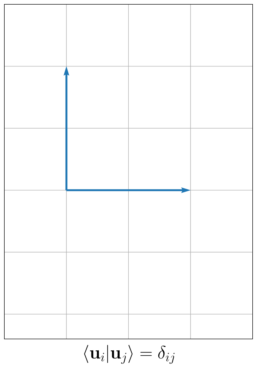
(a) Orthogonal

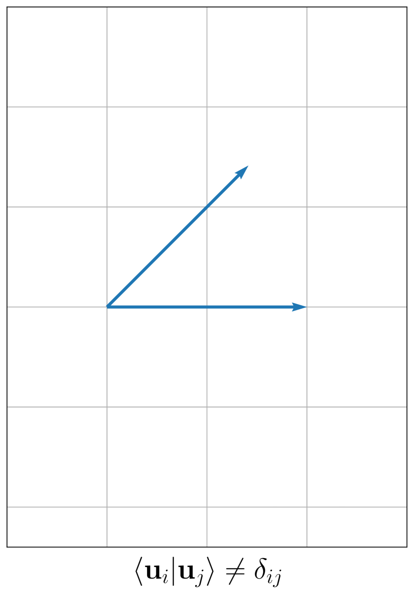
(b) Non-orthogonal

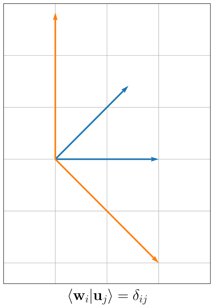
(c) Biorthogonal

Figure 1: Three types of bases for the 2D plane. (a) An orthogonal basis (unit overlap). (b) A non-orthogonal basis (non-unit overlap). (c) A biorthogonal basis. The primal/ket basis (blue) and the dual/bra basis (orange) are separate non-orthogonal bases for the plane. Together, they constitute a biorthogonal basis with unit overlap.

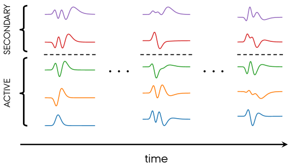
Figure 2: Schematic representation of an adaptive basis that is divided into active and secondary parts. Each vibrational mode has such a basis.

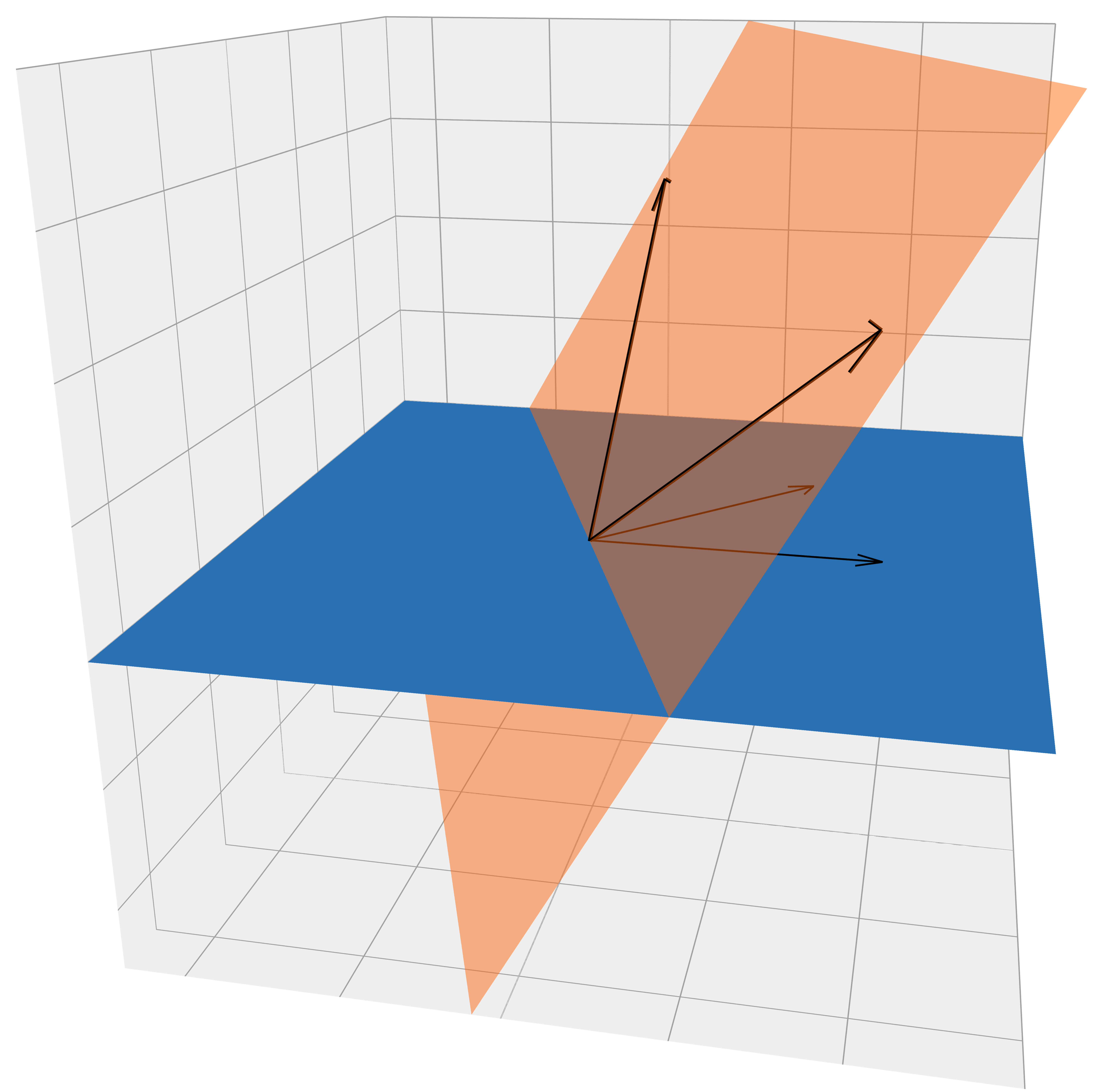
(a)

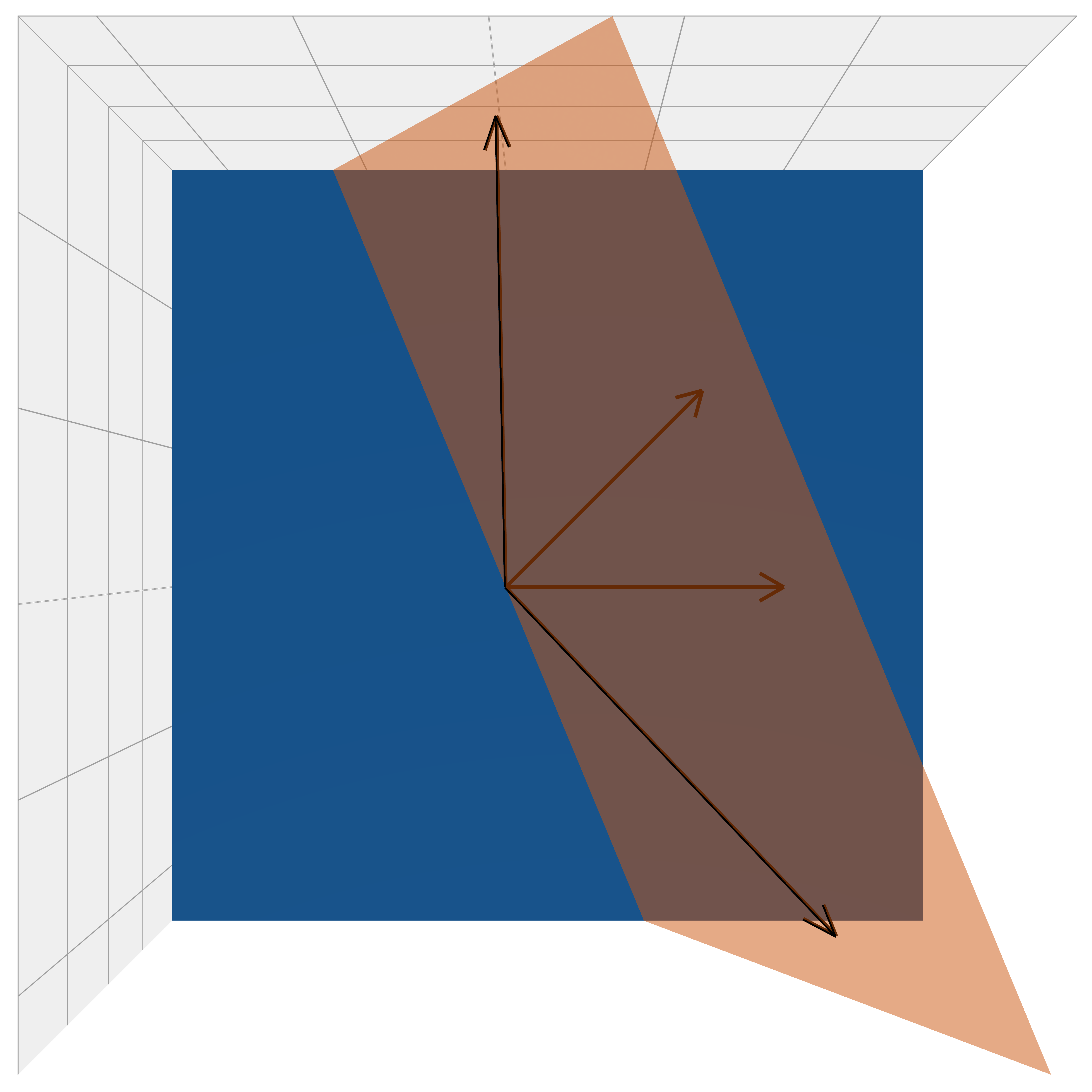
(b)

Figure 3: A biorthogonal set where the primal and dual bases do not span the same 2D planes. The set nevertheless has unit overlap, which can be seen by comparing the right-hand panel to Fig. 1(c).

We would like an alternative parameterization where the active dual/bra and primal/ket spaces are the same, but without restricting the active basis to be orthogonal. The first step towards such a parameterization is to understand that the exponential function $e^{\hat{\kappa}}$ has two roles: (i) choosing an active space and (ii) choosing a basis within that space. These roles are mixed together in the single exponential formulation, but they can be separated by introducing a double or split exponential parameterization:

$$e^{\hat{\kappa}}\rightarrow e^{\hat{\sigma}}e^{\hat{\kappa}},$$ (5a)

$$\hat{\sigma}=\sum_{m}{\sum_{pq}}^{(m)}\sigma^{m}_{{p}{q}}\,E^{m}_{{p}{q}},\quad\hat{\kappa}=\sum_{m}{\sum_{pq}}^{(m)}\kappa^{m}_{{p}{q}}\,E^{m}_{{p}{q}}.$$ (5b)

Here, the first factor ($e^{\hat{\sigma}}$) is an operator that changes the active space, while the second factor ($e^{\hat{\kappa}}$) changes the active basis (the order of the factors will be explained shortly). Equivalently, one can think of the factors as generating interspace and intraspace transformations, i.e. mixing between the active and secondary spaces and mixing within the active space. Such a separation can be realized by requiring a certain type of structure in the time derivative of the operators $\hat{\sigma}$ and $\hat{\kappa}$. The details for the general case (i.e. $\hat{\sigma}\neq 0$ and $\hat{\kappa}\neq 0$) can be worked out by using the Lie algebraic techniques of Ref. 26, but for now we will focus on the simple case where $\hat{\sigma}=0$ and $\hat{\kappa}=0$. At this point, the time derivatives are required to assume a particularly transparent structure, namely

$$\dot{\mathbf{\Sigma}}^{m} =\left[\begin{array}[]{c | c}\mspace{2.0mu}\mathbf{0}\mspace{3.0mu}{}&{}\mspace{3.0mu}\bm{*}\\ \hline\cr\mspace{2.0mu}\bm{*}\mspace{3.0mu}{}&{}\mspace{3.0mu}\mathbf{0}\mspace{2.0mu}{}\end{array}\right],$$ (6c)

$$\dot{\mathbf{K}}^{m} =\left[\begin{array}[]{c | c}\mspace{2.0mu}\bm{*}\mspace{3.0mu}{}&{}\mspace{3.0mu}\mathbf{0}\mspace{2.0mu}{}\\ \hline\cr\mspace{2.0mu}\mathbf{0}\mspace{3.0mu}{}&{}\mspace{3.0mu}\mathbf{0}\mspace{2.0mu}{}\end{array}\right],$$ (6f)

where the block structure refers to the active–secondary division. We have introduced the matrices $\mathbf{\Sigma}^{m}$ and $\mathbf{K}^{m}$ containing the $\sigma^{m}_{{p}{q}}$ and $\kappa^{m}_{{p}{q}}$ parameters, respectively, and used asterisks to indicate non-zero blocks. Regardless of the detailed structure, the basic operators transform as

$$a^{m\mspace{-0.5mu}\raisebox{0.90417pt}{$\scriptstyle\dagger$}}_{\mspace{0.0mu}q} \rightarrow\breve{a}^{m\mspace{-0.5mu}\raisebox{0.90417pt}{$\scriptstyle\dagger$}}_{\mspace{0.0mu}q} =e^{\hat{\sigma}}e^{\hat{\kappa}}\,a^{m\mspace{-0.5mu}\raisebox{0.90417pt}{$\scriptstyle\dagger$}}_{\mspace{0.0mu}q} e^{-\hat{\kappa}}e^{-\hat{\sigma}} ={\sum_{\bar{p}p}}^{(m)}a^{m\mspace{-0.5mu}\raisebox{0.90417pt}{$\scriptstyle\dagger$}}_{\mspace{0.0mu}\bar{p}}\exp(+\mathbf{\Sigma}^{m})_{\bar{p}p}\exp(+\mathbf{K}^{m})_{pq} ={\sum_{\bar{p}}}^{(m)}a^{m\mspace{-0.5mu}\raisebox{0.90417pt}{$\scriptstyle\dagger$}}_{\mspace{0.0mu}\bar{p}}\,\mathcal{U}_{\bar{p}q}^{m},$$ (7a)

$$a^{m}_{\mspace{0.0mu}p} \rightarrow\breve{b}^{m}_{\mspace{-1.0mu}p} =e^{\hat{\sigma}}e^{\hat{\kappa}}\,a^{m}_{\mspace{0.0mu}p} e^{-\hat{\kappa}}e^{-\hat{\sigma}} ={\sum_{\bar{q}q}}^{(m)}\exp(-\mathbf{K}^{m})_{pq}\exp(-\mathbf{\Sigma}^{m})_{q\bar{q}}\,a^{m}_{\mspace{0.0mu}\bar{q}} ={\sum_{\bar{q}}}^{(m)}\mathcal{W}_{p\bar{q}}^{m}\,a^{m}_{\mspace{0.0mu}\bar{q}},$$ (7b)

where we have defined matrices $\bm{\mathcal{U}}^{m}$ and $\bm{\mathcal{W}}^{m}$ holding the coefficients of the total transformation for mode $m$ (these matrices are of course the inverse of each other). It is important to note that the transformations by $\exp(+\mathbf{\Sigma}^{m})$ and $\exp(-\mathbf{\Sigma}^{m})$ are carried out first, contrary to what one might expect from the ordering of the product $e^{\hat{\sigma}}e^{\hat{\kappa}}$. The transformation that defines the active space thus precedes the one that defines a suitable basis within that space.

If we take $\hat{\sigma}$ and $\hat{\kappa}$ to be both anti-Hermitian (or both generic) we get an overall transformation that is unitary (or non-unitary) and completely equivalent to a single exponential transformation. We are, however, free to choose an anti-Hermitian $\hat{\sigma}$ and a generic $\hat{\kappa}$. This allows unitary transformations of the active space, and non-unitary transformations within the active space. In particular, the active bra and ket bases are not necessarily orthogonal, but they span the same space. The double exponential format is useable as it stands (i.e. one can propagate the matrices $\mathbf{K}^{m}$ and $\mathbf{\Sigma}^{m}$ as the time-dependent basis set parameters), but we find it convenient to do a slight reformulation. We are free to absorb the unitary transformation into the creators and annihilators and write Eqs. (7) as

$${\sum_{\bar{p}p}}^{(m)}a^{m\mspace{-0.5mu}\raisebox{0.90417pt}{$\scriptstyle\dagger$}}_{\mspace{0.0mu}\bar{p}}\exp(+\mathbf{\Sigma}^{m})_{\bar{p}p}\exp(+\mathbf{K}^{m})_{pq} ={\sum_{p}}^{(m)}\tilde{a}^{m\mspace{-0.5mu}\raisebox{0.90417pt}{$\scriptstyle\dagger$}}_{\mspace{0.0mu}p}\exp(+\mathbf{K}^{m})_{pq} =e^{\hat{\kappa}}\,\tilde{a}^{m\mspace{-0.5mu}\raisebox{0.90417pt}{$\scriptstyle\dagger$}}_{\mspace{0.0mu}q} e^{-\hat{\kappa}},$$ (8a)

$${\sum_{\bar{q}q}}^{(m)}\exp(-\mathbf{K}^{m})_{pq}\exp(-\mathbf{\Sigma}^{m})_{q\bar{q}}\,a^{m}_{\mspace{0.0mu}\bar{q}} ={\sum_{q}}^{(m)}\exp(-\mathbf{K}^{m})_{pq}\,\tilde{a}^{m}_{\mspace{0.0mu}q} =e^{\hat{\kappa}}\,\tilde{a}^{m}_{\mspace{0.0mu}p} e^{-\hat{\kappa}}.$$ (8b)

Although we have not changed the notation, the $\hat{\kappa}$ operator is now defined with respect to the moving creators $\tilde{a}^{m\mspace{-0.5mu}\raisebox{0.90417pt}{$\scriptstyle\dagger$}}_{\mspace{0.0mu}q}$:

$$\hat{\kappa}=\sum_{m}{\sum_{pq}}^{(m)}\kappa^{m}_{{p}{q}}\tilde{E}^{m}_{{p}{q}},\quad\tilde{E}^{m}_{{p}{q}}=\tilde{a}^{m\mspace{-0.5mu}\raisebox{0.90417pt}{$\scriptstyle\dagger$}}_{\mspace{0.0mu}p}\tilde{a}^{m}_{\mspace{0.0mu}q}.$$ (9)

These creators are themselves given by

$$\tilde{a}^{m\mspace{-0.5mu}\raisebox{0.90417pt}{$\scriptstyle\dagger$}}_{\mspace{0.0mu}p}={\sum_{\bar{p}}}^{(m)}a^{m\mspace{-0.5mu}\raisebox{0.90417pt}{$\scriptstyle\dagger$}}_{\mspace{0.0mu}\bar{p}}\exp(\mathbf{\Sigma}^{m})_{\bar{p}p}={\sum_{\bar{p}}}^{(m)}a^{m\mspace{-0.5mu}\raisebox{0.90417pt}{$\scriptstyle\dagger$}}_{\mspace{0.0mu}\bar{p}}V^{m}_{\mspace{-2.0mu}\bar{p}p},$$ (10)

where the matrix $\mathbf{V}^{m}$ is unitary and can be propagated in time rather than $\mathbf{\Sigma}^{m}$. The linear parameterization in terms of $\mathbf{V}^{m}$ is (in some ways) simpler than the exponential parameterization in terms of $\mathbf{\Sigma}^{m}$, but it requires the use of constraints, a point that we will return to later. The main motivation for using a linear-type parameterization for the unitary transformation is that it will allow us to introduce a secondary-space projection, which is convenient if the secondary space is large.

It is possible to also absorb the non-unitary transformation into the creators/annihilators from the outset, which would correspond to working explicitly in the breve basis of Eqs. (7) with the matrices $\bm{\mathcal{U}}^{m}$ and $\bm{\mathcal{W}}^{m}$ as the time-dependent parameters. This leads, however, to complicated constraints and less transparent derivations (as far as we can tell). We will therefore keep the exponential formulation for the non-unitary transformation for the time being and only describe an optional linearization at the end. In conclusion, we continue with a parameterization like

$$\ket{\Psi} =e^{\hat{\kappa}}\ket{\psi},$$ (11a)

$$\bra{\Psi^{\prime}} =\bra{\psi^{\prime}}e^{\hat{\kappa}},$$ (11b)

where $\ket{\psi}$, $\bra{\psi^{\prime}}$ and $\hat{\kappa}$ are expressed in terms of the moving creators of Eq. (9). With this choice, the $\mathbf{K}^{m}$ matrices always have the overall structure given by Eq. (6f) and the total basis set transformation is given by the matrices

$$\bm{\mathcal{U}}^{m}=\mathbf{V}^{m}\exp(+\mathbf{K}^{m})=\left[\begin{array}[]{c | c}\mathbf{V}_{\!\!\textsc{a}}^{m}}{&{\,}\mathbf{V}_{\!\textsc{s}}^{m}\rule{0.0pt}{10.33327pt}\end{array}\right]\left[\begin{array}[]{c | c}{\mathbf{U}^{m}_{\!\textsc{a}\textsc{a}}}{}&{\,}{\mathbf{0}}\rule{0.0pt}{10.33327pt}\\ \hline\cr{\mathbf{0}}{}&{\,}\mspace{6.0mu}{\mathbf{1}}{\mspace{6.0mu}}\rule{0.0pt}{10.33327pt}\end{array}\right],$$ (12d)

$$\bm{\mathcal{W}}^{m}=\exp(-\mathbf{K}^{m})\,\mathbf{V}^{m\dagger}=\left[\begin{array}[]{c | c}{\mathbf{W}^{m}_{\!\!\textsc{a}\textsc{a}}}{}&{\,}{\mathbf{0}}\rule{0.0pt}{10.33327pt}\\ \hline\cr{\mathbf{0}}{}&{\,}\mspace{6.0mu}{\mathbf{1}}{\mspace{6.0mu}}\rule{0.0pt}{10.33327pt}\end{array}\right]\left[\begin{array}[]{c}\mathbf{V}_{\!\!\textsc{a}}^{m\dagger}\\ \hline\cr\mathbf{V}_{\!\textsc{s}}^{m\dagger}\end{array}\right],$$ (12i)

where we have defined $\mathbf{U}^{m}=\exp(\mathbf{K}^{m})$ and $\mathbf{W}^{m}=\exp(-\mathbf{K}^{m})$ and used the block structure of $\mathbf{K}^{m}$. In particular, the active blocks of $\bm{\mathcal{U}}^{m}$ and $\bm{\mathcal{W}}^{m}$ are

$$\bm{\mathcal{U}}^{m}_{\!\textsc{a}} =\mathbf{V}^{m}_{\!\!\textsc{a}}\mathbf{U}^{m}_{\!\textsc{a}\textsc{a}},$$ (13a)

$$\bm{\mathcal{W}}^{m}_{\!\!\textsc{a}} =\mathbf{W}^{m}_{\!\!\textsc{a}\textsc{a}}\mathbf{V}^{m\dagger}_{\!\!\textsc{a}}.$$ (13b)

These matrices are exactly each other’s Moore–Penrose inverses,Weisstein (2008) which is another way of stating the fact that the active bra and ket spaces are the same, even though the active basis is not orthogonal. The Moore–Penrose inverse is unique whenever it exists, so the active bra basis is uniquely defined by the active ket basis (and vice versa).

We have obtained the Moore–Penrose structure in a particular way, namely by separating interspace and intraspace transformations, but this is not the only way. Returning to the double exponential format at the point $\hat{\sigma}=\hat{\kappa}=0$, we could also require

$$\dot{\mathbf{\Sigma}}^{m} =\left[\begin{array}[]{c | c}\mspace{2.0mu}\bm{*}\mspace{3.0mu}{}&{}\mspace{3.0mu}\bm{*}\\ \hline\cr\mspace{2.0mu}\bm{*}\mspace{3.0mu}{}&{}\mspace{3.0mu}\mathbf{0}\mspace{2.0mu}{}\end{array}\right],$$ (14c)

$$\dot{\mathbf{K}}^{m} =\left[\begin{array}[]{c | c}\mspace{2.0mu}\bm{*}\mspace{3.0mu}{}&{}\mspace{3.0mu}\mathbf{0}\mspace{2.0mu}{}\\ \hline\cr\mspace{2.0mu}\mathbf{0}\mspace{3.0mu}{}&{}\mspace{3.0mu}\mathbf{0}\mspace{2.0mu}{}\end{array}\right],$$ (14f)

with $\dot{\mathbf{\Sigma}}^{m}$ anti-Hermitian and $\dot{\mathbf{K}}^{m}$ Hermitian. This leads to a polar-type decompositionHall (2015) of the overall basis set transformation with $e^{\hat{\sigma}}$ unitary and $e^{\hat{\kappa}}$ positive definite, and where the latter factor is restricted to acting within the active space. We arrived at such a ‘restricted polar’ parameterization from a different starting point in Ref. 21, but the eom obtained were not fully bivariational. Although we did not observe any deterioration of accuracy, we did see some energy non-conversation as a symptom of the non-bivariational nature of the theory. It should be possible to derive a fully bivariational version of this theory, but we believe it would be rather complicated compared to the approach of separating interspace and intraspace transformations.

The idea of a double exponential basis set transformation has in fact been considered in ground state electronic structure theory. Köhn and OlsenKöhn and Olsen (2005) considered a ‘modified OCC’ method defined by a (bi)variationally optimized, unitary interspace transformation and a Brueckner-type intraspace transformation determined by projection. This method recovers the fci limit for ground state energies, but inherits the unphysical second-order poles in the bcc response function.Aiga, Sasagane, and Itoh (1994); Koch, Kobayashi, and Jørgensen (1994) It is also not clear to us how one would actually propagate a Brueckner-type transformation in time. Consequently, we do not consider the ‘modified occ’ Ansatz as an attractive choice for our purposes. We also mention the work of OlsenOlsen (2015) on ci-type expansions with non-orthogonal orbitals that are optimized using a polar-type product $e^{\hat{\sigma}}e^{\hat{\kappa}}$, where $\hat{\sigma}$ is anti-Hermitian (anti-symmetric) and $\hat{\kappa}$ is Hermitian (symmetric). Although this approach is highly relevant for the present discussion, it is not directly applicable in the context of wave functions that are explicitly time-dependent, complex-valued, and bivariational.

II.2 The Hamiltonian in second quantization

The first-quantized Hamiltonian can be written as

$$\hat{H}=\sum_{\mathbf{m}}\hat{H}^{\mathbf{m}},$$ (15)

where $\mathbf{m}$ is a mc, i.e. a set of modes. The notation means that a given term $\hat{H}^{\mathbf{m}}$ acts only on the modes $\mathbf{m}$. In the second-quantized formalism,Christiansen (2004) the Hamiltonian with respect to the primitive basis reads

$$H=\sum_{\mathbf{m}}{\sum_{\bm{\alpha}\bm{\beta}}}^{(\mathbf{m})}H^{\mathbf{m}}_{\bm{\alpha}\bm{\beta}}E^{\mathbf{m}}_{{\bm{\alpha}}{\bm{\beta}}},\quad E^{\mathbf{m}}_{{\bm{\alpha}}{\bm{\beta}}}=\prod_{m\in\mathbf{m}}E^{m}_{{\alpha^{m}}{\beta^{m}}},$$ (16)

with integrals

$$H^{\mathbf{m}}_{\bm{\alpha}\bm{\beta}}=\Big{\langle}\prod_{m\in\mathbf{m}}\chi^{m}_{\alpha^{m}}\Big{|}\hat{H}^{\mathbf{m}}\Big{|}\prod_{m\in\mathbf{m}}\chi^{m}_{\beta^{m}}\Big{\rangle}.$$ (17)

Here, $\bm{\alpha}$ and $\bm{\beta}$ are vectors of primitive indices, which are henceforth represented by lowercase Greek letters. Each operator $\hat{H}^{\mathbf{m}}$ is typically represented as a sum of products of one-mode operators, in which case the integrals factor into products of one-mode integrals. In the basis defined by the moving creators of Eq. (9), the operator looks like

$$H=\sum_{\mathbf{m}}{\sum_{\mathbf{p}\mathbf{q}}}^{(\mathbf{m})}\tilde{H}^{\mathbf{m}}_{\mathbf{p}\mathbf{q}}\tilde{E}^{\mathbf{m}}_{{\mathbf{p}}{\mathbf{q}}},$$ (18)

$$\tilde{H}^{\mathbf{m}}_{\mathbf{p}\mathbf{q}}={\sum_{\bm{\alpha}\bm{\beta}}}^{(\mathbf{m})}\left(\prod_{m\in\mathbf{m}}V^{m*}_{\mspace{-2.0mu}\alpha^{m}p^{m}}\right)H^{\mathbf{m}}_{\bm{\alpha}\bm{\beta}}\left(\prod_{m\in\mathbf{m}}V^{m}_{\mspace{-2.0mu}\beta^{m}q^{m}}\right),$$ (19)

but we remark that Eqs. (16) and (18) are strictly equal. We will also encounter the similarity transformed Hamiltonian

$$\bar{H}=e^{-\hat{\kappa}}He^{\hat{\kappa}}=\sum_{\mathbf{m}}{\sum_{\mathbf{p}\mathbf{q}}}^{(\mathbf{m})}\breve{H}^{\mathbf{m}}_{\mathbf{p}\mathbf{q}}\tilde{E}^{\mathbf{m}}_{{\mathbf{p}}{\mathbf{q}}}.$$ (20)

The creators and annihilators are still in the basis of Eq. (9), but the integrals have been transformed once more:

$$\breve{H}^{\mathbf{m}}_{\mathbf{p}\mathbf{q}} ={\sum_{\bar{\mathbf{p}}\bar{\mathbf{q}}}}^{(\mathbf{m})}\left(\prod_{m\in\mathbf{m}}\exp(-\mathbf{K}^{m})_{p^{m}\bar{p}^{m}}\right)\tilde{H}^{\mathbf{m}}_{\bar{\mathbf{p}}\bar{\mathbf{q}}}\left(\prod_{m\in\mathbf{m}}\exp(\mathbf{K})_{\bar{q}^{m}q^{m}}\right)$$

$$={\sum_{\bm{\alpha}\bm{\beta}}}^{(\mathbf{m})}\left(\prod_{m\in\mathbf{m}}\mathcal{W}^{m}_{p^{m}\alpha^{m}}\right)H^{\mathbf{m}}_{\bm{\alpha}\bm{\beta}}\left(\prod_{m\in\mathbf{m}}\mathcal{U}^{m}_{\beta^{m}q^{m}}\right).$$ (21)

II.3 The time-dependent bivariational principle

The tdbvp in its original formArponen (1983); Kvaal (2012) considers a complex-valued Lagrangian,

$$\quad\mathcal{L}=\langle\Psi^{\prime}|(i\partial_{t}-H)|\Psi\rangle,$$ (22)

and the corresponding complex-valued action,

$$\mathcal{S}=\int_{t_{0}}^{t_{1}}\mathcal{L}\differential{t}.$$ (23)

The bra and ket states are taken to be independent. Requiring the action to be stationary ($\delta\mathcal{S}=0$) with respect to arbitrary and independent variations that vanish at the end points is equivalent to the Schrödinger equation and its dual:

$$i\ket{\dot{\Psi}}=H\ket{\Psi},$$ (24a)

$$-i\bra{\dot{\Psi}^{\prime}}=\bra{\Psi^{\prime}}H.$$ (24b)

In practice, the bra and ket states are parameterized in terms of a set of complex parameters $z_{i}$ and the stationary condition is then equivalent to a set of ele,

$$0 =\partialderivative{\mathcal{L}}{z_{i}}-\derivative{t}\partialderivative{\mathcal{L}}{\dot{z}_{i}}.$$ (25)

These equations are consistent as long as the Lagrangian is holomorphic (complex analytic) in the parameters (in particular, complex conjugation must not appear in $\mathcal{L}$). This subtle point is mentioned by KvaalKvaal (2012) and discussed in some detail in Ref. 23 and its Appendix A. Although it may seem like a technicality, it has some important consequences for the kinds of parameterizations that can be permitted. As an example, the complex-valued Lagrangian rules out the use of an orthogonal basis (in that case the bra basis is simply the complex conjugate of the ket basis).

Instead, we may consider a manifestly real Lagrangian,

$$\bar{\mathcal{L}}=\mathrm{Re}(\mathcal{L})=\tfrac{1}{2}(\mathcal{L}+\mathcal{L}^{*}),$$ (26)

where we allow the parameterization of the bra and ket states to be non-holomorphic, i.e. we allow the states to depend on a set of parameters $\mathbf{z}$ as well as the complex conjugate parameters $\mathbf{z}^{*}$. The total set of independent variational parameters is thus $\{\mathbf{z},\mathbf{z}^{*}\}$ (it is also possible to use $\mathrm{Re}(\mathbf{z})$ and $\mathrm{Im}(\mathbf{z})$ as the independent parameters, but this is somewhat inconvenient in practical derivations). The evolution of the parameters is determined by making the real action functional $\bar{\mathcal{S}}=\mathrm{Re}(\mathcal{S})$ stationary, which is equivalent to a set of ele for the parameters $\mathbf{z}$ and $\mathbf{z}^{*}$ separately, i.e.

$$0 =\partialderivative{\bar{\mathcal{L}}}{z_{i}}-\derivative{t}\partialderivative{\bar{\mathcal{L}}}{\dot{z}_{i}},$$ (27a)

$$0 =\partialderivative{\bar{\mathcal{L}}}{z_{i}^{*}}-\derivative{t}\partialderivative{\bar{\mathcal{L}}}{\dot{z}_{i}^{*}}.$$ (27b)

These equations are each other’s complex conjugate, since the Lagrangian is real. It is thus sufficient to solve one of them.

We note that if $\mathcal{L}$ depends on a certain parameter $z_{k}$, but not on the complex conjugate $z_{k}^{*}$, then the real-valued tdbvp reduces to the complex-valued tdbvp for that particular parameter:

$$0 =\partialderivative{\bar{\mathcal{L}}}{z_{k}}-\derivative{t}\partialderivative{\bar{\mathcal{L}}}{\dot{z}_{k}}$$

$$=\frac{1}{2}\left(\partialderivative{\mathcal{L}}{z_{k}}-\derivative{t}\partialderivative{\mathcal{L}}{\dot{z}_{k}}\right)+\frac{1}{2}\left(\partialderivative{\mathcal{L}}{z_{k}^{*}}-\derivative{t}\partialderivative{\mathcal{L}}{\dot{z}_{k}^{*}}\right)^{\!*}$$

$$=\frac{1}{2}\left(\partialderivative{\mathcal{L}}{z_{k}}-\derivative{t}\partialderivative{\mathcal{L}}{\dot{z}_{k}}\right).$$ (28)

II.4 Parameterization and constraints

As explained in Sec. II.1, we consider a moving orthonormal basis or, equivalently, a set of moving creators

$$\tilde{a}^{m\mspace{-0.5mu}\raisebox{0.90417pt}{$\scriptstyle\dagger$}}_{\mspace{0.0mu}p}={\sum_{\alpha}}^{(m)}a^{m\mspace{-0.5mu}\raisebox{0.90417pt}{$\scriptstyle\dagger$}}_{\mspace{0.0mu}\alpha}V^{m}_{\mspace{-2.0mu}\alpha p}.$$ (29)

At this point we consider all basis functions (active and secondary) explicitly, so that the matrix $\mathbf{V}^{m}$ containing the expansion coefficients is a square, unitary matrix.

The time-dependent basis must be orthonormal at any given time, which is a constraint on the basis set. In addition, the time derivative of this constraint must vanish at any given time (this is a so-called consistency conditionDirac (1950); Ohta (2000, 2004)). Using matrix notation, the constraints and consistency conditions read

$$\mathbf{V}^{m\dagger}\,\mathbf{V}^{m}=\mathbf{1}^{m},$$ (30a)

$$\mathbf{0}=\dot{\mathbf{V}}^{m\dagger}\,\mathbf{V}^{m}+\mathbf{V}^{m\dagger}\,\dot{\mathbf{V}}^{m}.$$ (30b)

The latter equation holds trivially if

$$\dot{\mathbf{V}}^{m\dagger}\,\mathbf{V}^{m} =+i\mathbf{G}^{m},$$ (31a)

$$\mathbf{V}^{m\dagger}\,\dot{\mathbf{V}}^{m} =-i\mathbf{G}^{m},$$ (31b)

where $\mathbf{G}^{m}$ is a Hermitian but otherwise arbitrary matrix, which we call the constraint matrix. Using Eq. (31b) and the fact that $\mathbf{V}^{m}$ is unitary we see that

$$i\dot{\mathbf{V}}^{m}=\mathbf{V}^{m}\mathbf{G}^{m},$$ (32)

which means that the constraint matrix acts as a generator for the time evolution of $\mathbf{V}^{m}$.

It is convenient at this point to divide the time-dependent basis into an active basis indexed by $t$, $u$, $v$, $w$ and a secondary basis indexed by $x$, $y$. We use $\alpha$, $\beta$ to denote primitive indices, while $p$, $q$, $r$, $s$ denote generic time-dependent indices. The division of the basis induces a block structure in $\mathbf{V}^{m}$ and $\mathbf{G}^{m}$:

$$\mathbf{V}^{m}=\left[\begin{array}[]{c | c}{\mathbf{V}^{m}_{\!\!\textsc{a}}}&\,\mathbf{V}^{m}_{\!\textsc{s}}\rule[-4.30554pt]{0.0pt}{0.0pt}\end{array}\right],$$ (33b)

$$\mathbf{G}^{m}=\left[\begin{array}[]{c | c}{\mathbf{G}^{m}_{\textsc{a}\textsc{a}}}&{\mathbf{G}^{m}_{\textsc{a}\textsc{s}}}\rule{0.0pt}{10.33327pt}\\ \hline\cr{\mathbf{G}^{m}_{\textsc{s}\textsc{a}}}&{\mathbf{G}^{m}_{\textsc{s}\textsc{s}}}\rule{0.0pt}{10.33327pt}\end{array}\right].$$ (33e)

Right-hand subscripts a and s are used to indicate the active and secondary blocks of matrices that have one primitive and one time-dependent index. Matrices with two time-dependent indices have four blocks: (i) active–active (aa); (ii) active–secondary (as); (iii) secondary–active (sa); and (iv) secondary–secondary (ss).

In order to ensure that $\mathbf{G}^{m}$ generates only interspace transformations, we enforce the block structure of Eq. (6c), i.e. we set

$$\mathbf{G}^{m}\equiv\left[\begin{array}[]{c | c}\mathbf{0}&{\mathbf{G}^{m}_{\textsc{a}\textsc{s}}}\rule{0.0pt}{10.33327pt}\\ \hline\cr{\mathbf{G}^{m}_{\textsc{s}\textsc{a}}}&\mathbf{0}\rule{0.0pt}{10.33327pt}\end{array}\right].$$ (36)

The $\mathbf{G}^{m}_{\textsc{s}\textsc{s}}$ block is always redundant and can safely be set to zero, whereas the $\mathbf{G}^{m}_{\textsc{a}\textsc{a}}$ block would ordinarily not be redundant. It is, however, not needed in our case since we have explicitly introduced a separate parameterization for the intraspace transformations. In conclusion, we only retain the $\mathbf{G}^{m}_{\textsc{s}\textsc{a}}$ and $\mathbf{G}^{m}_{\textsc{a}\textsc{s}}=(\mathbf{G}^{m}_{\textsc{s}\textsc{a}})^{\dagger}$ blocks, which mix the active and secondary spaces. It is important to note that this particular Ansatz for $\mathbf{G}^{m}$ generates unitary transformations that change the active space without determining an appropriate active basis. That is to say that the columns of $\mathbf{V}^{m}_{\!\!\textsc{a}}$ span the active space, but they are generally not good basis vectors in themselves.

To summarize: We will consider rather general bra and ket parameterizations of the form

$$\ket{\Psi(\bm{\alpha},\bm{\kappa},\mathbf{V})} =e^{\hat{\kappa}}\ket{\psi(\bm{\alpha},\mathbf{V})},$$ (37a)

$$\bra{\Psi^{\prime}(\bm{\alpha},\bm{\kappa},\mathbf{V}^{*})} =\bra{\psi^{\prime}(\bm{\alpha},\mathbf{V}^{*})}e^{-\hat{\kappa}},$$ (37b)

with

$$\hat{\kappa}=\sum_{m}{\sum_{tu}}^{(m)}\kappa^{m}_{{t}{u}}\tilde{E}^{m}_{{t}{u}},\quad\tilde{E}^{m}_{{t}{u}}=\tilde{a}^{m\mspace{-0.5mu}\raisebox{0.90417pt}{$\scriptstyle\dagger$}}_{\mspace{0.0mu}t}\tilde{a}^{m}_{\mspace{0.0mu}u}.$$ (38)

The $\kappa^{m}_{{t}{u}}$ parameters are collected in vectors $\bm{\kappa}^{m}_{\textsc{a}\textsc{a}}$ or matrices $\mathbf{K}^{m}_{\textsc{a}\textsc{a}}$ depending on context (the vector $\bm{\kappa}_{\textsc{a}\textsc{a}}$ contains all $\kappa^{m}_{{t}{u}}$ for all modes). $\bm{\alpha}$ is a vector of complex configurational or correlation parameters (e.g. cc amplitudes) and $\mathbf{V}=\{\mathbf{V}^{m}\}$ denotes the basis set coefficients. It is important to note that the ket state depends on the coefficients themselves, while the bra state depends on the complex conjugate coefficients, $\mathbf{V}^{*}$.

II.5 Equations of motion

II.5.1 Lagrangian

In order to compute the Lagrangian, Eq. (26), we will start by considering the action of the time-derivative on a single Hartree product:

$$\ket{\Phi_{\mathbf{s}}}=\prod_{m=1}^{M}\tilde{a}^{m\mspace{-0.5mu}\raisebox{0.90417pt}{$\scriptstyle\dagger$}}_{\mspace{0.0mu}s^{m}}\ket{\mathrm{vac}}$$ (39)

It is easy to see by applying the product rule that the time derivative acts as a one-particle operator on a single Hartree product (the same holds for a single Slater determinant). In fact, one can show (see Ref. 21) that

$$\langle\Phi_{\mathbf{r}}|\partial_{t}|\Phi_{\mathbf{s}}\rangle=\langle\Phi_{\mathbf{r}}|(-iG)|\Phi_{\mathbf{s}}\rangle$$ (40)

where the so-called constraint operator,

$$G=\sum_{m}{\sum_{pq}}^{(m)}g^{m}_{{p}{q}}\,\tilde{E}^{m}_{{p}{q}},$$ (41)

is constructed from the constraint matrix elements. Next, we introduce an active-space resolution of identity and write the bra and ket as

$$\ket{\Psi} =\sum_{\mu}\ket{\mu}\mspace{-2.0mu}\mspace{-2.0mu}\braket{\mu}{\Psi} \equiv\sum_{\mu}c_{\mu}(\bm{\alpha},\bm{\kappa})\ket{\mu(\mathbf{V})},$$ (42a)

$$\bra{\Psi^{\prime}} =\sum_{\mu}\braket{\Psi^{\prime}}{\mu}\mspace{-2.0mu}\mspace{-2.0mu}\bra{\mu} \equiv\sum_{\mu}{c^{\prime}}_{\mspace{-6.0mu}\mu}(\bm{\alpha},\bm{\kappa})\bra{\mu(\mathbf{V}^{*})}.$$ (42b)

The summations run over all Hartree products (or Slater determinants) within the active space. Defining $\mathbf{y}=(\bm{\alpha},\bm{\kappa})$, we find that

$$\langle\Psi^{\prime}|\partial_{t}|\Psi\rangle =\bra{\Psi^{\prime}}\sum_{\mu}\big{(}\dot{c}_{\mu}\ket{\mu}+c_{\mu}\ket{\dot{\mu}}\big{)}$$

$$=\bra{\Psi^{\prime}}\sum_{\mu j}\dot{y}_{j}\partialderivative{c_{\mu}}{y_{j}}\ket{\mu}+\bra{\Psi^{\prime}}\sum_{\mu}c_{\mu}(-iG)\ket{\mu}$$

$$=\sum_{j}\dot{y}_{j}\Big{\langle}\Psi^{\prime}\mspace{2.0mu}\Big{|}\mspace{1.5mu}\partialderivative{\Psi}{y_{j}}\Big{\rangle}-i\langle\Psi^{\prime}|G|\Psi\rangle$$ (43)

and, consequently, that

$$\mathcal{L} =\langle\Psi^{\prime}|(i\partial_{t}-H)|\Psi\rangle$$

$$=i\sum_{j}\dot{y}_{j}\Big{\langle}\Psi^{\prime}\mspace{2.0mu}\Big{|}\mspace{1.5mu}\partialderivative{\Psi}{y_{j}}\Big{\rangle}-\langle\Psi^{\prime}|(H-G)|\Psi\rangle$$

$$\equiv\mathcal{I}-\mathcal{H}^{\prime}.$$ (44)

The first term depends only on $\mathbf{y}$ and $\dot{\mathbf{y}}$, while the second term depends on $\mathbf{y}$, $\mathbf{V}$, $\dot{\mathbf{V}}$ and $\mathbf{V}^{*}$.

II.5.2 Basis set coefficients

Equation (II.5.1) has exactly the same form as the Lagrangian in Ref. 23, so we simply restate the result from that paper: The ele

$$0 =\partialderivative{\bar{\mathcal{L}}}{V^{m}_{\mspace{-2.0mu}\alpha q}}-\derivative{t}\partialderivative{\bar{\mathcal{L}}}{\dot{V}^{m}_{\mspace{-2.0mu}\alpha q}}$$ (45)

lead to the following equations for ${\mathbf{G}^{m}_{\textsc{s}\textsc{a}}}$:

$${\mathbf{G}^{m}_{\textsc{s}\textsc{a}}}\;\mathbb{H}[\bm{{\mathchoice{\raisebox{1.0pt}{$\displaystyle\rho$}}{\raisebox{1.0pt}{$\textstyle\rho$}}{\raisebox{1.0pt}{$\scriptstyle\rho$}}{\raisebox{1.0pt}{$\scriptscriptstyle\rho$}}}}^{m}_{\!\textsc{a}\textsc{a}}] =\tfrac{1}{2}({\tilde{\mathbf{F}}^{m}_{\!\textsc{s}\textsc{a}}}+{\tilde{\mathbf{F}}^{\prime m\dagger}_{\!\!\textsc{a}\textsc{s}}})$$ (46a)

$$=\tfrac{1}{2}\mathbf{V}^{m\dagger}_{\!\textsc{s}}(\check{\mathbf{F}}^{m}_{\!\!\textsc{a}}+\check{\mathbf{F}}^{\prime m\dagger}_{\!\!\textsc{a}}).$$ (46b)

Here, $\mathbb{H}[\,\cdot\,]$ denotes the Hermitian part of a square matrix. We have defined one-particle density matrices,

$$\rho^{m}_{pq}=\langle\Psi^{\prime}|\tilde{E}^{m}_{{q}{p}}|\Psi\rangle={\sum_{\bar{p}\bar{q}}}^{(m)}\exp(\mathbf{K}^{m})_{p\bar{p}}\,\langle\psi^{\prime}|\tilde{E}^{m}_{{\bar{q}}{\bar{p}}}|\psi\rangle\exp(-\mathbf{K}^{m})_{\bar{q}q},$$ (47)

generalized mean-field or Fock matrices,

$$\tilde{F}^{\prime m}_{{q}{p}} =\langle\Psi^{\prime}|[H,\tilde{a}^{m\mspace{-0.5mu}\raisebox{0.90417pt}{$\scriptstyle\dagger$}}_{\mspace{0.0mu}p}]\tilde{a}^{m}_{\mspace{0.0mu}q}|\Psi\rangle,$$ (48a)

$$\tilde{F}^{m}_{{q}{p}} =\langle\Psi^{\prime}|\tilde{a}^{m\mspace{-0.5mu}\raisebox{0.90417pt}{$\scriptstyle\dagger$}}_{\mspace{0.0mu}p}[\tilde{a}^{m}_{\mspace{0.0mu}q},H]|\Psi\rangle,$$ (48b)

and partially transformed mean-field matrices,

$$\check{F}^{\prime m}_{{q}{\alpha}} =\partialderivative{\mathcal{H}}{V^{m}_{\mspace{-2.0mu}\alpha q}} =\langle\Psi^{\prime}|[H,a^{m\mspace{-0.5mu}\raisebox{0.90417pt}{$\scriptstyle\dagger$}}_{\mspace{0.0mu}\alpha}]\tilde{a}^{m}_{\mspace{0.0mu}q}|\Psi\rangle,$$ (49a)

$$\check{F}^{m}_{{\alpha}{q}} =\partialderivative{\mathcal{H}}{V^{m*}_{\mspace{-2.0mu}\alpha q}} =\langle\Psi^{\prime}|\tilde{a}^{m\mspace{-0.5mu}\raisebox{0.90417pt}{$\scriptstyle\dagger$}}_{\mspace{0.0mu}q}[a^{m}_{\mspace{0.0mu}\alpha},H]|\Psi\rangle.$$ (49b)

These matrices are partially transformed in the sense that one index refers to the primitive basis, while the other refers to the orthogonal tilde basis. Equation (47) relates the density matrix of the $\hat{\kappa}$-transformed states to that of the untransformed states in a simple way, which is useful for practical implementations. One also needs to address the $\hat{\kappa}$-transformation inside the mean-field matrix elements, and some care is needed in the partially transformed case since it involves creators and annihilators in different bases. It is always possible to write the (partially transformed) mean fields in terms of contractions of (partially transformed) Hamiltonian integrals and density matrices. The $\hat{\kappa}$-transformation adds extra one-index contractions that can be absorbed into either the integrals or the density matrices, depending on implementation details. Our approach is outlined in Appendix A.

Unlike Ref. 23, we dot not solve any equations for $\mathbf{G}^{m}_{\textsc{a}\textsc{a}}$, since these constraint elements are simply not part of our parameterization. Dropping the mode index for clarity, Eq. (32) now reads

$$i\left[\begin{array}[]{c | c}\dot{\mathbf{V}}_{\!\!\textsc{a}}}{&{\,}\dot{\mathbf{V}}_{\!\textsc{s}}\rule{0.0pt}{10.33327pt}\end{array}\right]=\left[\begin{array}[]{c | c}\mathbf{V}_{\!\!\textsc{a}}}{&{\,}\mathbf{V}_{\!\textsc{s}}\rule{0.0pt}{10.33327pt}\end{array}\right]\left[\begin{array}[]{c | c}{\mathbf{0}}{}&{\,}{\mathbf{G}_{\textsc{a}\textsc{s}}}\rule{0.0pt}{10.33327pt}\\ \hline\cr{\mathbf{G}_{\textsc{s}\textsc{a}}}{}&{\,}{\mathbf{0}}\rule{0.0pt}{10.33327pt}\end{array}\right],$$ (54)

or, focusing on the active block,

$$i\dot{\mathbf{V}}_{\!\!\textsc{a}} =\mathbf{V}_{\!\textsc{s}}\,{\mathbf{G}_{\textsc{s}\textsc{a}}}$$

$$=\mathbf{V}_{\!\textsc{s}}^{\phantom{\dagger}}\mspace{-2.0mu}\mathbf{V}_{\!\textsc{s}}^{\dagger}\tfrac{1}{2}(\check{\mathbf{F}}_{\!\!\textsc{a}}+\check{\mathbf{F}}^{\prime\dagger}_{\!\!\textsc{a}})\,\mathbb{H}[\bm{{\mathchoice{\raisebox{1.0pt}{$\displaystyle\rho$}}{\raisebox{1.0pt}{$\textstyle\rho$}}{\raisebox{1.0pt}{$\scriptstyle\rho$}}{\raisebox{1.0pt}{$\scriptscriptstyle\rho$}}}}_{\!\textsc{a}\textsc{a}}]^{-1}$$

$$=\tfrac{1}{2}\mathbf{Q}(\check{\mathbf{F}}_{\!\!\textsc{a}}+\check{\mathbf{F}}^{\prime\dagger}_{\!\!\textsc{a}})\,\mathbb{H}[\bm{{\mathchoice{\raisebox{1.0pt}{$\displaystyle\rho$}}{\raisebox{1.0pt}{$\textstyle\rho$}}{\raisebox{1.0pt}{$\scriptstyle\rho$}}{\raisebox{1.0pt}{$\scriptscriptstyle\rho$}}}}_{\!\textsc{a}\textsc{a}}]^{-1}$$ (55)

The secondary-space projector $\mathbf{Q}$ is given by

$$\mathbf{Q}=\mathbf{V}_{\!\textsc{s}}^{\phantom{\dagger}}\mspace{-2.0mu}\mathbf{V}_{\!\textsc{s}}^{\dagger}=\mathbf{1}-\mathbf{V}_{\!\!\textsc{a}}^{\phantom{\dagger}}\mspace{-2.0mu}\mathbf{V}_{\!\!\textsc{a}}^{\dagger}$$ (56)

and allows us to propagate $\mathbf{V}_{\!\!\textsc{a}}$ without reference to secondary-space quantities.

II.5.3 $\bm{\alpha}$ and $\bm{\kappa}$ parameters

The complex Lagrangian $\mathcal{L}$ is an analytic function of $\mathbf{y}$ and $\dot{\mathbf{y}}$ ($\mathbf{y}^{*}$ and $\dot{\mathbf{y}}^{*}$ never appear), so the ele

$$0 =\partialderivative{\bar{\mathcal{L}}}{y_{i}}-\derivative{t}\partialderivative{\bar{\mathcal{L}}}{\dot{y}_{i}}$$ (57)

are equivalent to

$$0 =\partialderivative{\mathcal{L}}{y_{i}}-\derivative{t}\partialderivative{\mathcal{L}}{\dot{y}_{i}}.$$ (58)

This set of equations is identical to that studied in Ref. 26, except for the fact that the Hamiltonian appearing in $\mathcal{L}$ is modified by $G$; see Eq. (II.5.1). The operator $G$ does not depend on $\mathbf{y}$ or $\dot{\mathbf{y}}$, so this difference has no consequence for the variational calculation. In fact, the $G$ term drops altogether due to Eq. (36) and the usual killer conditions. We will thus proceed with $\mathcal{H}^{\prime}\rightarrow\mathcal{H}$. It is not difficult to showHøjlund, Zoccante, and Christiansen (2023) that Eq. (58) is equivalent to

$$i\sum_{j}\mathcal{M}_{ij}\dot{y}_{j} =\partialderivative{\mathcal{H}}{y_{i}},$$ (59)

where

$$\mathcal{M}_{ij}=\Big{\langle}\partialderivative{\Psi^{\prime}}{y_{i}}\mspace{2.0mu}\Big{|}\mspace{1.5mu}\partialderivative{\Psi}{y_{j}}\Big{\rangle}-\Big{\langle}\partialderivative{\Psi^{\prime}}{y_{j}}\mspace{2.0mu}\Big{|}\mspace{1.5mu}\partialderivative{\Psi}{y_{i}}\Big{\rangle}.$$ (60)

Further derivations lead to

$$i\dot{\bm{\alpha}} =\mathbf{M}^{-1}\mathbf{h}^{\prime},$$ (61a)

$$\big{(}\mathbf{C}+\mathbf{A}^{\mspace{-3.0mu}\mathsf{T}}\mathbf{M}^{-1}\mathbf{A}\big{)}\tilde{\mathbf{g}} =\big{(}\mathbf{f}+\mathbf{A}^{\mspace{-3.0mu}\mathsf{T}}\mathbf{M}^{-1}\mathbf{h}\big{)}.$$ (61b)

The matrices and vectors are defined according to

$$M_{ij} =\Big{\langle}\partialderivative{\psi^{\prime}}{\alpha_{i}}\mspace{2.0mu}\Big{|}\mspace{1.5mu}\partialderivative{\psi}{\alpha_{j}}\Big{\rangle}-\Big{\langle}\partialderivative{\psi^{\prime}}{\alpha_{j}}\mspace{2.0mu}\Big{|}\mspace{1.5mu}\partialderivative{\psi}{\alpha_{i}}\Big{\rangle}$$ (62a)

$$A_{{i}({m^{\prime}}{v}{w})} =\partialderivative{\alpha_{i}}\langle\psi^{\prime}|\tilde{E}^{m^{\prime}}_{{v}{w}}|\psi\rangle,$$ (62b)

$$C_{({m}{t}{u})({m^{\prime}}{v}{w})} =\langle\psi^{\prime}|[\tilde{E}^{m^{\prime}}_{{v}{w}},\tilde{E}^{m}_{{t}{u}}]|\psi\rangle,$$ (62c)

$$f_{(m{t}{u})} =\langle\psi^{\prime}|[\bar{H},\tilde{E}^{m}_{{t}{u}}]|\psi\rangle,$$ (62d)

$$h_{i} =\partialderivative{\alpha_{i}}\langle\psi^{\prime}|\bar{H}|\psi\rangle,$$ (62e)

$$h_{i}^{\prime} =\partialderivative{\alpha_{i}}\langle\psi^{\prime}|(\bar{H}-\tilde{G})|\psi\rangle,$$ (62f)

$$\bar{H} =e^{-\hat{\kappa}}He^{\hat{\kappa}}.$$ (62g)

The operator $\tilde{G}$, which is determined by Eq. (61b), is given by

$$\tilde{G} =\sum_{m}{\sum_{vw}}^{(m)}\tilde{g}^{m}_{vw}\,\tilde{E}^{m}_{{v}{w}}$$

$$=ie^{-\hat{\kappa}}\derivative{e^{\hat{\kappa}}}{t}$$

$$=i\sum_{m}{\sum_{tu}}^{(m)}\dot{\kappa}^{m}_{{t}{u}}\,e^{-\hat{\kappa}}\partialderivative{e^{\hat{\kappa}}}{\kappa^{m}_{{t}{u}}}$$

$$\equiv i\sum_{m}{\sum_{tu}}^{(m)}\dot{\kappa}^{m}_{{t}{u}}\,D^{m}_{tu}$$

$$=i\sum_{m}{\sum_{tuvw}}^{(m)}\dot{\kappa}^{m}_{{t}{u}}\,d^{m}_{({t}{u})({v}{w})}\tilde{E}^{m}_{{v}{w}},$$ (63)

or, in matrix-vector notation,

$$\tilde{\mathbf{g}}^{m}=i(\mathbf{D}^{m})^{\mspace{-3.0mu}\mathsf{T}}\dot{\bm{\kappa}}^{m}_{\textsc{a}\textsc{a}}.$$ (64)

Reference 26 shows how this equation can be solved for $\dot{\bm{\kappa}}^{m}_{\textsc{a}\textsc{a}}$ without explicitly constructing and inverting the large ($N_{\!\textsc{a}}^{2}\times N_{\!\textsc{a}}^{2}$) matrix $\mathbf{D}^{m}$. We note that it is also perfectly possible to propagate the matrices

$$\mathbf{U}^{m}_{\!\textsc{a}\textsc{a}} =\exp(\mathbf{K}^{m}_{\textsc{a}\textsc{a}}),$$ (65a)

$$\mathbf{W}^{m}_{\!\!\textsc{a}\textsc{a}} =\exp(-\mathbf{K}^{m}_{\textsc{a}\textsc{a}}),$$ (65b)

rather than $\mathbf{K}^{m}$ itself. The second line of Eq. (II.5.3) implies

$$\tilde{\mathbf{G}}^{m}=i\mathbf{W}^{m}_{\!\!\textsc{a}\textsc{a}}\dot{\mathbf{U}}^{m}_{\!\textsc{a}\textsc{a}}=-i\dot{\mathbf{W}}^{m}_{\!\!\textsc{a}\textsc{a}}\mathbf{U}^{m}_{\!\textsc{a}\textsc{a}}$$ (66)

or, using the fact that $\mathbf{W}^{m}$ and $\mathbf{U}^{m}$ are each other’s inverses,

$$\dot{\mathbf{U}}^{m}_{\!\textsc{a}\textsc{a}} =-i\mathbf{U}^{m}_{\!\textsc{a}\textsc{a}}\tilde{\mathbf{G}}^{m},$$ (67a)

$$\dot{\mathbf{W}}^{m}_{\!\!\textsc{a}\textsc{a}} =+i\tilde{\mathbf{G}}^{m}\mathbf{W}^{m}_{\!\!\textsc{a}\textsc{a}}.$$ (67b)

The exponential and linear formulations are of course fully equivalent and require the solution of the same set of linear equations, Eq. (61b).

II.6 Working equations for the CC Ansatz

We now state the working equations in greater detail with emphasis on the cc Ansatz:

$$\ket{\Psi}=e^{\hat{\kappa}}\ket{\psi}=e^{\hat{\kappa}}e^{T}\ket{\Phi},$$ (68a)

$$\bra{\Psi^{\prime}}=\bra{\psi^{\prime}}e^{-\hat{\kappa}}=\bra{\Phi}Le^{-T}e^{-\hat{\kappa}}.$$ (68b)

The operators $T$ and $L$ are given by

$$T =\sum_{\mu}t_{\mu}\tilde{\tau}_{\mu} =t_{0}+T_{2}+T_{3}+\ldots$$ (69a)

$$L =\sum_{\mu}l_{\mu}\tilde{\tau}_{\mu}^{\dagger} =l_{0}+L_{2}+L_{3}+\ldots$$ (69b)

where it should be noted that the single excitations are omitted since they are redundant with the basis set transformation generated by $\hat{\kappa}$.Kvaal (2012); Sato et al. (2018); Madsen et al. (2020a); Pedersen, Koch, and Hättig (1999); Pedersen, Fernández, and Koch (2001) The excitation operators $\tilde{\tau}_{\mu}$ and the reference $\ket{\Phi}$ are defined in terms of the moving creators $\tilde{a}^{m\mspace{-0.5mu}\raisebox{0.90417pt}{$\scriptstyle\dagger$}}_{\mspace{0.0mu}v}$, and we can thus consider Eqs. (68) as an nocc-type expansion inside an evolving active space. This Ansatz is able to reproduce the complete wave function expansion within the active space,Myhre (2018) which means that exact active-space densities and mean fields are obtained when $T$ and $L$ are not truncated. Exact densities and mean fields in turn generate the exact evolution of the active space itself according to Eq. (II.5.2). The Ansatz thus reproduces the mctdh limit in the vibrational case and the mctdhf limit in the electronic structure case.

The amplitude eom can of course be derived by applying the tdbvp directly to the cc Ansatz, but in our general framework we order the amplitudes like $\bm{\alpha}=(\mathbf{t},\mathbf{l})$ and apply Eq. (62a) to find that

$$\mathbf{M}=\left[\begin{array}[]{c | c}\mathbf{0}&-\mathbf{1}\\ \hline\cr+\mathbf{1}&\mathbf{0}\end{array}\right],\quad\mathbf{M}^{-1}=\left[\begin{array}[]{c | c}\mathbf{0}&+\mathbf{1}\\ \hline\cr-\mathbf{1}&\mathbf{0}\end{array}\right].$$ (74)

Having obtained $\mathbf{M}^{-1}$, Eq. (61a) readily yields the result:

$$i\dot{t}_{\mu} =+\langle\mu|e^{-T}(\bar{H}-\tilde{G})|\psi\rangle,$$ (75a)

$$i\dot{l}_{\mu} =-\langle\psi^{\prime}|[\bar{H}-\tilde{G},\tilde{\tau}_{\mu}]|\psi\rangle.$$ (75b)

The non-unitary basis set transformation is determined by Eq. (61b),

$$\big{(}\mathbf{C}+\mathbf{A}^{\mspace{-3.0mu}\mathsf{T}}\mathbf{M}^{-1}\mathbf{A}\big{)}\tilde{\mathbf{g}}=\big{(}\mathbf{f}+\mathbf{A}^{\mspace{-3.0mu}\mathsf{T}}\mathbf{M}^{-1}\mathbf{h}\big{)},$$ (76)

which we rewrite simply as

$$\mathbf{C}^{\prime}\tilde{\mathbf{g}}=\mathbf{f}^{\prime}.$$ (77)

The primes indicate the inclusion of the terms depending on $\mathbf{A}$. Referring to Eqs. (62), one easily computes the elements of $\mathbf{C}^{\prime}$ and $\mathbf{f}^{\prime}$:

$$C^{\prime}_{({m}{t}{u})({m^{\prime}}{v}{w})}=\langle\psi^{\prime}|[\tilde{E}^{m^{\prime}}_{{v}{w}},\tilde{E}^{m}_{{t}{u}}]|\psi\rangle\\ +\sum_{\mu}\Big{(}\langle\psi^{\prime}|[\tilde{E}^{m}_{{t}{u}},\tilde{\tau}_{\mu}]|\psi\rangle\langle\mu|e^{-T}\tilde{E}^{m^{\prime}}_{{v}{w}}|\psi\rangle-\langle\psi^{\prime}|[\tilde{E}^{m^{\prime}}_{{v}{w}},\tilde{\tau}_{\mu}]|\psi\rangle\langle\mu|e^{-T}\tilde{E}^{m}_{{t}{u}}|\psi\rangle\Big{)}$$ (78)

and

$$f^{\prime}_{(m{t}{u})}=\langle\psi^{\prime}|[\bar{H},\tilde{E}^{m}_{{t}{u}}]|\psi\rangle\\ +\sum_{\mu}\Big{(}\langle\psi^{\prime}|[\tilde{E}^{m}_{{t}{u}},\tilde{\tau}_{\mu}]|\psi\rangle\langle\mu|e^{-T}\bar{H}|\psi\rangle-\langle\psi^{\prime}|[\bar{H},\tilde{\tau}_{\mu}]|\psi\rangle\langle\mu|e^{-T}\tilde{E}^{m}_{{t}{u}}|\psi\rangle\Big{)}.$$ (79)

The active space is divided into occupied ($i,j,\ldots$) and virtual ($a,b,\ldots$) subspaces, which means that index pairs $tu$ can be divided into four types: $ai$ (up), $ia$ (down), $ab$ (forward) and $ij$ (passive). A particular feature of vibrational structure theory is that each mode has only a single occupied index, something that is useful in concrete implementations. Using $u$, $d$, $f$ and $p$ to label the four types of index pairs induces a block structure in the linear equations. Many of these blocks can be shown to vanish,Madsen et al. (2020a) so that we are left with

$$\left[\begin{array}[]{c | c | c | c}\mathbf{0}&{{}^{ud}\mathbf{C}}&\mathbf{0}&\mathbf{0}\rule{0.0pt}{12.91663pt}\\ \hline\cr{{}^{du}\mathbf{C}}&{{}^{dd}\mathbf{C}}^{\prime}&\mathbf{0}&\mathbf{0}\rule{0.0pt}{12.91663pt}\\ \hline\cr\mathbf{0}&\mathbf{0}&\mathbf{0}&\mathbf{0}\rule{0.0pt}{12.91663pt}\\ \hline\cr\mathbf{0}&\mathbf{0}&{\hskip 7.3194pt}\mathbf{0}}{&\hskip 7.3194pt\mathbf{0}{\hskip 6.45831pt}\rule{0.0pt}{12.91663pt}\end{array}\right]\left[\begin{array}[]{c}{{}^{u}\tilde{\mathbf{g}}}\rule{0.0pt}{12.91663pt}\\ \hline\cr{{}^{d}\tilde{\mathbf{g}}}\rule{0.0pt}{12.91663pt}\\ \hline\cr{{}^{f\!}\tilde{\mathbf{g}}}\rule{0.0pt}{12.91663pt}\\ \hline\cr{{}^{p}\tilde{\mathbf{g}}}\rule{0.0pt}{12.91663pt}\end{array}\right]=\left[\begin{array}[]{c}{{}^{u}\mathbf{f}}\rule{0.0pt}{12.91663pt}\\ \hline\cr{{}^{d}\mathbf{f}^{\prime}}\rule{0.0pt}{12.91663pt}\\ \hline\cr\mathbf{0}\rule{0.0pt}{12.91663pt}\\ \hline\cr\mathbf{0}\rule{0.0pt}{12.91663pt}\end{array}\right].$$ (92)

Evidently, the forward and passive blocks of $\tilde{\mathbf{g}}$ are redundant. This is not surprising since these blocks generate transformations within the virtual and occupied spaces, respectively. Such intraspace transformations are redundant for a wide range of time-dependent and time-independent wave function Ansätze, including cc. One can in fact determine the redundancies from the outset by geometric arguments (see e.g. Refs.19 and 36), but we find it satisfying and reassuring to see that they also show up in a concrete derivation.

The non-redundant equations now read

$${{}^{ud}\mathbf{C}}\,{{}^{d}\tilde{\mathbf{g}}}={{}^{u}\mathbf{f}},$$ (93a)

$${{}^{du}\mathbf{C}}\,{{}^{u}\tilde{\mathbf{g}}}+{{}^{dd}\mathbf{C}}^{\prime}\,{{}^{d}\tilde{\mathbf{g}}}={{}^{d}\mathbf{f}^{\prime}},$$ (93b)

and can be solved as

$${{}^{d}\mathbf{g}}=({{}^{ud}\mathbf{C}})^{-1}\,{{}^{u}\mathbf{f}},$$ (94a)

$${{}^{u}\mathbf{g}}=({{}^{du}\mathbf{C}})^{-1}({{}^{d}\mathbf{f}^{\prime}}-{{}^{dd}\mathbf{C}}^{\prime}\,{{}^{d}\mathbf{g}}).$$ (94b)

We observe the following: (i) the up and down equations can be solved sequentially and (ii) the matrices ${{}^{ud}\mathbf{C}}$ and ${{}^{du}\mathbf{C}}$ are diagonal in the mode index [see Eq. (62c)], meaning they can be inverted one mode at a time. Equations (94) thus consist of $2M$ linear systems of dimension $N_{\textsc{v}}N_{\textsc{o}}\times N_{\textsc{v}}N_{\textsc{o}}=N_{\textsc{v}}\times N_{\textsc{v}}$, where $M$ is the number of vibrational modes. The symbols $N_{\textsc{v}}$ and $N_{\textsc{o}}=1$ denote the number of virtual and occupied functions per mode, and we assume, for simplicity, that $N_{\textsc{v}}$ is the same for all modes (this is often not the case in practical calculations). The fact that the linear equations are up-down and mode-mode decoupled constitutes a large reduction in the computational effort compared to the orthogonal case,Højlund, Zoccante, and Christiansen (2024) where one generally (except at the doubles level) has to solve a single linear system of dimension $2MN_{\textsc{v}}N_{\textsc{o}}\times 2MN_{\textsc{v}}N_{\textsc{o}}=2MN_{\textsc{v}}\times 2MN_{\textsc{v}}$. In electronic structure theory, only the up-down decoupling applies, and the reduction from one system of dimension $2N_{\textsc{v}}N_{\textsc{o}}\times 2N_{\textsc{v}}N_{\textsc{o}}$ (orthogonal orbitals) to two systems of dimension $N_{\textsc{v}}N_{\textsc{o}}\times N_{\textsc{v}}N_{\textsc{o}}$ (biorthogonal orbitals) is less striking, although still significant.

III IMPLEMENTATION

The sTDMVCC method has been implemented in the midas,Christiansen et al. (2023) which includes an array of methods for solving the time-independent and time-dependent vibrational Schrödinger equations and for constructing pes. At the two-mode coupling level (sTDMVCC$[2]$/H2, i.e. $T=T_{2}$ and $H=H_{1}+H_{2}$), we have simply adapted the efficient TDMVCC$[2]$/H2 implementation of Ref. 38, which offers a cubic-scaling computational effort. For general coupling levels in $T$ and $H$ we adapt the original tdmvcc code,Madsen et al. (2020a) which is based on the fsmr implementation of Ref. 39. This is a FCI-type code, so the computational cost scales exponentially with respect to system size. Such a scaling is of course prohibitive for practical usage, but the fsmr code has nevertheless been instrumental for testing and benchmarking new cc variants with limited programming effort.

To avoid possible (near-)singularities in the one-mode density matrices [see Eq.(II.5.2)], we use a regularization scheme based on svd:

$$\bm{{\mathchoice{\raisebox{1.0pt}{$\displaystyle\rho$}}{\raisebox{1.0pt}{$\textstyle\rho$}}{\raisebox{1.0pt}{$\scriptstyle\rho$}}{\raisebox{1.0pt}{$\scriptscriptstyle\rho$}}}}_{\!\textsc{a}\textsc{a}}=\mathbf{X}\mathbf{\Sigma}\mathbf{Y}^{\dagger}\rightarrow\mathbf{X}\big{(}\mathbf{\Sigma}+\epsilon\exp(-\mathbf{\Sigma}/\epsilon)\big{)}\mathbf{Y}^{\dagger}.$$ (95)

Here, $\epsilon$ is a small regularization parameter (typically, $\epsilon=10^{-8}$). We rarely observe singularities in the main body of a simulation, but they do occur close to $t=0$ when using a vscf initial state or some other initial state that has active basis functions with exactly zero occupation. The same kind of regularization is used for inverting the individual blocks of ${{}^{ud}\mathbf{C}}$ and ${{}^{du}\mathbf{C}}$ in Eqs. (94). Finally, we modify the secondary-space projector of Eq. (56) according to

$$\mathbf{Q}=\mathbf{1}-\mathbf{V}_{\!\!\textsc{a}}^{\phantom{\dagger}}\mspace{-2.0mu}\mathbf{V}_{\!\!\textsc{a}}^{\dagger}\rightarrow\mathbf{1}-\mathbf{V}_{\!\!\textsc{a}}^{\phantom{\dagger}}(\mathbf{V}_{\!\!\textsc{a}}^{\dagger}\mathbf{V}_{\!\!\textsc{a}}^{\phantom{\dagger}})^{-1}\mathbf{V}_{\!\!\textsc{a}}^{\dagger}.$$ (96)

This guarantees that $\mathbf{Q}$ remains a proper projector even if the columns of $\mathbf{V}_{\!\!\textsc{a}}$ are not strictly orthonormal.

IV NUMERICAL EXAMPLES

We consider three examples in order to study the numerical stability and convergence properties of the sTDMVCC method: (i) ivr in water, (ii) the intramolecular proton transfer in a 6D salicylaldimine model,Polyak, Allan, and Worth (2015) and (iii) the dynamics after an $S_{1}\rightarrow S_{0}$ transition in a 5D trans-bithiophene model.Madsen et al. (2019) We employ basis set division (i.e., $N_{\!\textsc{a}}<N$) in all cases and compare with mctdh reference calculations as well as TDMVCC, rpTDMVCC, and oTDMVCC calculations. The eom are integrated using the dop853Hairer, Nørsett, and Wanner (2009) algorithm with tight absolute and relative tolerances for controlling the step size ($\tau_{\mathrm{abs}}=\tau_{\mathrm{rel}}=10^{-12}$). Density matrices are regularized using $\epsilon=10^{-8}$.

We take the physical expectation value of a Hermitian operator $\Omega$ to be

$$\langle\Omega\rangle=\mathrm{Re}\langle\Psi^{\prime}|\Omega|\Psi\rangle.$$ (97)

The corresponding imaginary part has no physical or experimental meaning as such, but it can be used to assess how well the wave function agrees with the exact limit where the imaginary part vanishes identically. We will thus write $\langle\Omega\rangle_{\mathrm{Re}}=\mathrm{Re}\langle\Psi^{\prime}|\Omega|\Psi\rangle$ and $\langle\Omega\rangle_{\mathrm{Im}}=\mathrm{Im}\langle\Psi^{\prime}|\Omega|\Psi\rangle$ when comparing the real and imaginary parts.

We also report acf computed asHansen et al. (2019)

$$S(t)=\braket{\Psi^{\prime}(0)}{\Psi(t)},$$ (98)

and, occasionally, basis set non-orthogonality defined as

$$\eta_{\mathrm{ket}}^{m}=||(\bm{\mathcal{U}}^{m}_{\!\textsc{a}})^{\dagger}(\bm{\mathcal{U}}^{m}_{\!\textsc{a}})-\mathbf{1}||,$$ (99a)

$$\eta_{\mathrm{bra}}^{m}=||(\bm{\mathcal{W}}^{m}_{\!\!\textsc{a}})(\bm{\mathcal{W}}^{m}_{\!\!\textsc{a}})^{\dagger}-\mathbf{1}||,$$ (99b)

where $||\cdot||$ is the Frobenius norm.

IV.1 Water

The first example is the ivr in water after exciting the symmetric stretch to $n=2$. We model this process by taking the $[0,2,0]$ state on the harmonic part of the pes as the initial state, followed by relaxation on the anharmonic and coupled pes. The calculation is repeated at the MCTDH, rpTDMVCC[2–3], oTDMVCC[2–3], sTDMVCC[2–3], and TDMVCC[2–3] levels with $N=20$ primitive modals per mode and a range of $N_{\!\textsc{a}}$ from $2$ to $20$. The propagation time is set to $20\,000\text{\,}\mathrm{a}\mathrm{u}$ ($\sim$$484\text{\,}\mathrm{f}\mathrm{s}$), but the number of integrator steps is capped at $90\,000$ in order to allow the program to terminate in an orderly fashion if the step size drops by a large amount.

IV.1.1 Numerical stability

All simulations proceed in an inconspicuous and stable manner, except at the TDMVCC[2] and TDMVCC[3] levels. These calculations suffer from the kind of instability that we first described in Ref. 21, as illustrated by Fig. 4. Figure 4(a) shows the integrator step size as a function of time for the TDMVCC[2] calculations with varying $N_{\!\textsc{a}}$. Whenever $N_{\!\textsc{a}}<N=20$, the step size eventually drops, making the equations virtually impossible to integrate. We observe, furthermore, that the sharp drop in step size correlates with a sharp increase in the amplitude vector norms [Figs. 4(b) and 4(c)]. Looking at Fig. 4, it appears that the breakdown happens suddenly and without warning, but the ket-state non-orthogonality [Fig. 5] shows that this is not quite the case. Here, we note a steady build-up of non-orthogonality followed by a violent increase that eventually leads to breakdown. It should be emphasized that this only happens when $N_{\!\textsc{a}}<N$, i.e. when the active bra and ket functions are allowed to span different spaces.

Similar problematic behavior is observed for TDMVCC[3] (see Figs. S1 and S2 in the supplementary material), while all remaining calculations run to completion without any problems (see Figs. S3–S14).

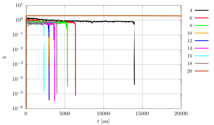
(a)

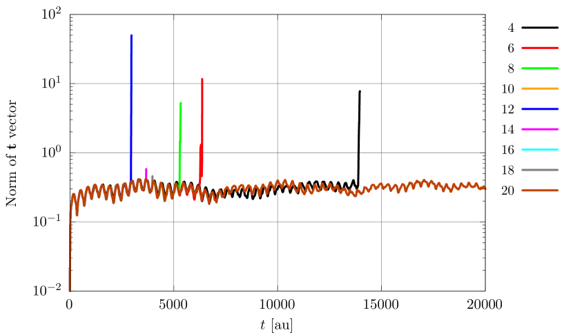
(b)

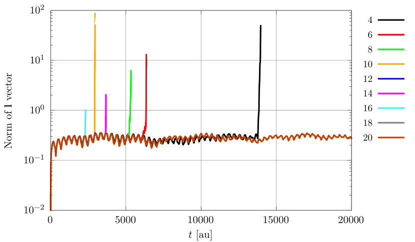
(c)

Figure 4: ivr in water at the TDMVCC[2] level with $N=20$ and a range of $N_{\!\textsc{a}}$ (as indicated by the figure legends). (a) Integrator step size. (b) Norm of $\mathbf{t}$ vector. (c) Norm of $\mathbf{l}$ vector.

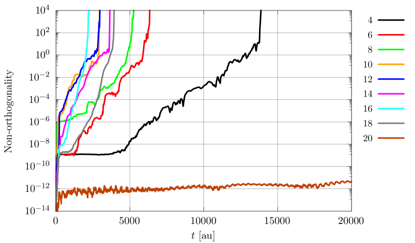
Figure 5: ivr in water at the TDMVCC[2] level with $N=20$ and a range of $N_{\!\textsc{a}}$ (as indicated by the figure legends). Ket non-orthogonality for mode $m=2$ (bend).

IV.1.2 acf

One might fear that the erratic numerical behavior of the TDMVCC calculations would also lead to an erratic description of observables. This is, however, not the case, as exemplified by Fig. 6, which shows the acf at the MCTDH, TDMVCC[2], sTDMVCC[2], oTDMVCC[2], and rpTDMVCC[2] levels of theory with $N=20$ and $N_{\!\textsc{a}}=6$. All cc variants agree closely with each other, and they reproduce the mctdh reference result quite well. This shows that the cc Ansatz as such is well suited for describing the dynamics at hand. Nevertheless, the TDMVCC[2] calculation breaks down at $t=$6369\text{\,}\mathrm{a}\mathrm{u}$$, while the remaining variants remain stable. We interpret this as a sign that the TDMVCC instability is not caused by the physics of the problem or by shortcomings of cc expansion in itself, but by the mathematical peculiarities of the TDMVCC basis set.

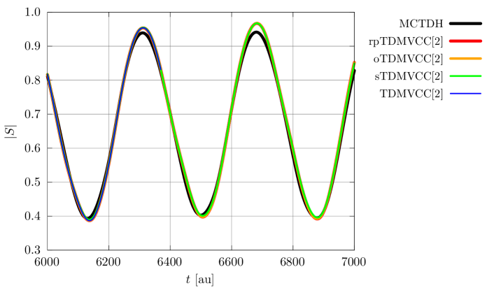
Figure 6: ivr in water at the MCTDH, TDMVCC[2], sTDMVCC[2], oTDMVCC[2], and rpTDMVCC[2] levels with $N=20$ and $N_{\!\textsc{a}}=6$. acf. Note that the TDMVCC[2] trace terminates at $t=$6369\text{\,}\mathrm{a}\mathrm{u}$$.

IV.2 6D salicylaldimine

Our second example is the intra-molecular proton transfer in salicylaldimine. This is an asymmetric double-well system with the lower well corresponding to the enol tautomer, which is more stable than the keto tautomer. We use the six-dimensional model pes from Ref. 40, which includes the modes labelled as $Q_{1}$, $Q_{10}$, $Q_{11}$, $Q_{13}$, $Q_{32}$, and $Q_{36}$ ($Q_{1}$ is the double-well mode). The initial state is a Gaussian wave packet placed just on the enol side of the barrier, but with an energy lower than the barrier height (see Refs. 40 and 44 for details). Crossing the barrier is thus classically forbidden and any flux over the barrier is solely due to tunneling.

The primitive basis for the calculation is obtained in the following way: Initially, a large B-spline basis is used for the double-well mode, while the remaining modes are described by 21 harmonic oscillator functions each. This basis is then transformed to a set of orthonormal vscf modals. For the double-well mode, we use the lowest 30 vscf modals as the primitive basis, while the remaining modes use all 21 vscf modals. The initial active modals are simply the $N_{\!\textsc{a}}=3$ lowest vscf modals for each mode. We do not expect the calculations to be fully converged with respect to $N_{\!\textsc{a}}$, but we note that our results are very similar to Ref. 44. Even if $N_{\!\textsc{a}}$ is not quite converged, this has no effect on the comparison between methods.

The total simulation time is $20\,000\text{\,}\mathrm{a}\mathrm{u}$ ($\sim$$484\text{\,}\mathrm{f}\mathrm{s}$), which is significantly longer than the $4200\text{\,}\mathrm{a}\mathrm{u}$ ($\sim$$100\text{\,}\mathrm{f}\mathrm{s}$) of Refs. 40 and 44. We have prioritized long simulations in order to assess numerical stability at long integration times. The calculation is repeated at the MCTDH, rpTDMVCC[2–6], oTDMVCC[2–6], sTDMVCC[2–6], and TDMVCC[2–6] levels.

IV.2.1 Numerical stability

Stability problems are observed for TDMVCC[2–4] as demonstrated by the integrator step size in Fig. 7. TDMVCC[5] and TDMVCC[6] remain stable within the time interval we have considered, but it is quite possible that they will fail at even longer integration times. The remaining cc variants integrate smoothly to completion and are not shown here (see Figs. S15–S17).

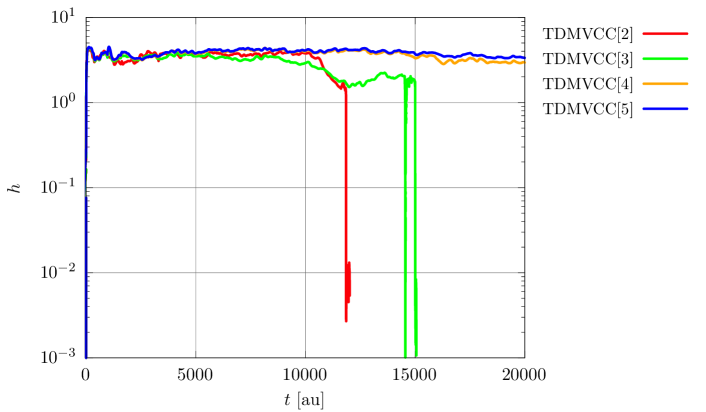
Figure 7: Integrator step size for 6D salicylaldimine at the TDMVCC[2–6] levels. The TDMVCC[2], TDMVCC[3], and TDMVCC[4] calculations terminated at $t=$6540\text{\,}\mathrm{a}\mathrm{u}$$, $t=$4989\text{\,}\mathrm{a}\mathrm{u}$$, and $t=$13\,413\text{\,}\mathrm{a}\mathrm{u}$$, respectively.

IV.2.2 Expectation values

The flux over the transition state (which is the zero of all coordinates) can be quantified by the flux operatorBeck et al. (2000) for mode $Q_{1}$ at the point $Q_{1}=0$:

$$F_{1}=i[\hat{H},\Theta(Q_{1})]=-\frac{i}{2}\left(\partialderivative{Q_{1}}\delta(Q_{1})+\delta(Q_{1})\partialderivative{Q_{1}}\right).$$ (100)

Here, $\Theta(Q_{1})$ is the Heaviside step function, $\delta(Q_{1})$ is the Dirac delta function, and the second expression holds only in rectilinear coordinates.Madsen et al. (2020b) Negative flux corresponds to the wave function crossing from the enol side to the keto side and vice versa.

Figure 8 shows the flux for sTDMVCC[2–6] compared to the MCTDH result. The flux is a sensitive property, and the double-well system is rather challenging, so we are able to see clear differences between different excitation levels. We find the quality of the sTDMVCC results to be quite acceptable already at the doubles level, but sTDMVCC[5] is in fact needed to get results that lie on top of MCTDH. Convergence can most likely be improved by a flexible excitation-space scheme similar to that of Ref. 44, where one includes, for example, all triple excitations involving the double-well mode in addition to all double excitations.

To the unaided eye, the other cc variants appear similar to sTDMVCC (see Figs. S18–S20), so we turn to the average absolute error [Fig. 9(a)] for a definite ranking. The eom are initially somewhat difficult to integrate due to the singular density matrices of the vscf initial state, resulting in oscillations of the absolute error at short times. We thus exclude the first $50\text{\,}\mathrm{a}\mathrm{u}$ from the averaging. The averaging is terminated at $t=$4989\text{\,}\mathrm{a}\mathrm{u}$$ (where TDMVCC[3] fails) in order to obtain an unbiased comparison. We observe that oTDMVCC does not converge to MCTDH, although this deficiency only shows up at the quintuple and sextuple levels. The remaining variants do converge, and the convergence patterns are very similar. In practical calculations on salicylaldimine or similar systems, one would thus not observe significant differences in quality between the methods.

As an additional check on the cc wave functions, we report the average value of $|\langle F_{1}\rangle_{\mathrm{Im}}|$ divided by the average value of $|\langle F_{1}\rangle_{\mathrm{Re}}|$ [Fig. 9(b)]. This provides a simple measure of the relative magnitude of the unphysical imaginary part. For the rpTDMVCC, sTDMVCC, and TDMVCC methods, which all allow non-unitary basis set transformations within the active space, the imaginary part goes to zero when the cluster expansion becomes complete. This is not the case for the oTDMVCC method, which is another clear sign that the orthogonal hierarchy cannot reproduce the exact solution correctly. Expectation values of the displacement coordinates behave similarly (see Figs. S21–S50).

It is also interesting to note that the unphysical imaginary part decreases quite slowly as a function of excitation level (rpTDMVCC and sTDMVCC) or not at all (oTDMVCC). This pattern differs qualitatively from the error in $\langle F_{1}\rangle$ [Fig. 9(a)], which improves quite steadily with respect to excitation level.

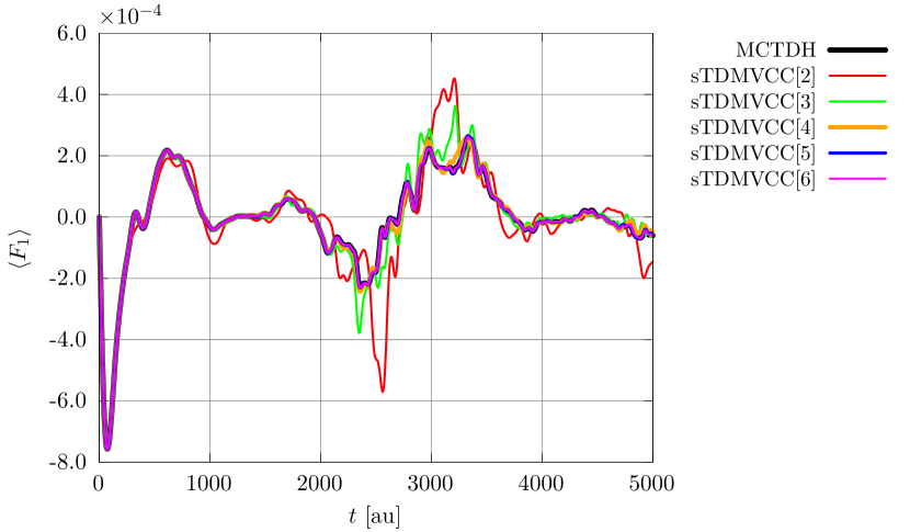
(a)

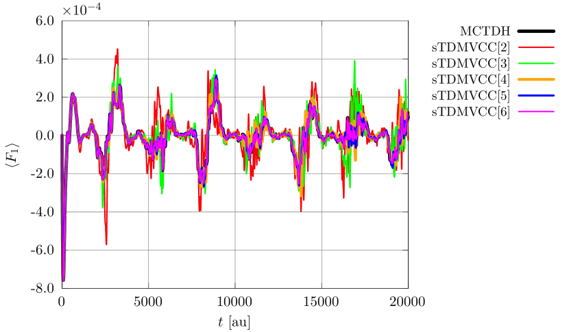
(b)

Figure 8: Expectation value $\langle F_{1}\rangle$ for 6D salicylaldimine at the MCDTH and sTDMVCC[2–6] levels. (a) Short times. (b) Full time interval.

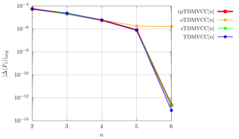
(a) Average error

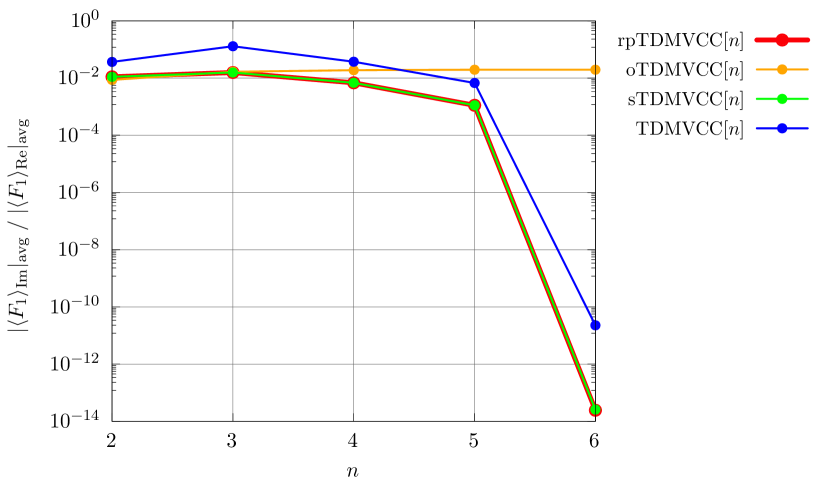
(b) Average imaginary vs. real part

Figure 9: Expectation value $\langle F_{1}\rangle$ for 6D salicylaldimine at the rpTDMVCC[2–6], sTDMVCC[2–6], oTDMVCC[2–6] and TDMVCC[2–6] levels. (a) Average error relative to MCTDH. (b) Average imaginary part divided by average real part. The averaging has been done over the time interval from $t=$50\text{\,}\mathrm{a}\mathrm{u}$$ to $t=$4989\text{\,}\mathrm{a}\mathrm{u}$$.

IV.2.3 Energy conservation

The physical energy $E=\mathrm{Re}(\mathcal{H})=\mathrm{Re}\langle\Psi^{\prime}|H|\Psi\rangle$ [Fig. 10(a)] is always conserved for the fully bivariational methods, i.e. TDMVCC, oTDMVCC, and sTDMVCC, which is of course reassuring. In contrast, rpTDMVCC does not conserve energy, except when the cluster expansion becomes complete. We take this as an unfortunate symptom of the non-bivariational nature of this method.

The imaginary part of the Hamiltonian function, $\mathrm{Im}(\mathcal{H})$, has no experimental significance, but it reveals some interesting and fundamental differences between methods that are complex bivariational (based on the complex-valued Lagrangian $\mathcal{L}$) and methods that are real bivariational (based on the real-valued Lagrangian $\bar{\mathcal{L}}$). For a complex bivariational method (such as TDMVCC), the dynamics is generated by the complex-valued Hamiltonian function $\mathcal{H}$. This entails conservation of $\mathcal{H}$ and thus of $\mathrm{Im}(\mathcal{H})$, which is confirmed by Fig. 10(b). The dynamics of real bivariational methods (such as oTDMVCC and sTDMVCC) is generated by the real-valued Hamiltonian function $\mathrm{Re}(\mathcal{H})$, which implies conservation of $\mathrm{Re}(\mathcal{H})$. We cannot expect $\mathrm{Im}(\mathcal{H})$ to be conserved, unless the wave function reproduces the complete-active-space solution exactly. Indeed, Fig. 10(b) shows that oTDMVCC never conserves $\mathrm{Im}(\mathcal{H})$, while sTDMVCC conserves $\mathrm{Im}(\mathcal{H})$ in the exact limit. We remark that rpTDMVCC behaves much like sTDMVCC, but in this case the analysis is less clear since rpTDMVCC is not fully bivariational in either the real or the complex sense.

(a) Real part

(b) Imaginary part

Figure 10: Energy conservation for 6D salicylaldimine at the rpTDMVCC[2–6], sTDMVCC[2–6], oTDMVCC[2–6] and TDMVCC[2–6] levels. (a) Average real part (this is the physical energy). (b) Average imaginary part. The averaging has been done over the time interval from $t=$50\text{\,}\mathrm{a}\mathrm{u}$$ to $t=$4989\text{\,}\mathrm{a}\mathrm{u}$$.

IV.3 5D trans-bithiophene

The third and final example is the $S_{1}\rightarrow S_{0}$ transition in a reduced-dimensional trans-bithiophene model that includes five modes labelled as $Q_{10}$, $Q_{12}$, $Q_{19}$, $Q_{34}$, and $Q_{41}$ (see Ref. 41 for details on the selection of modes). We obtain the initial state as the vscf ground state on the $S_{1}$ surface. The wave packet is then placed on the $S_{0}$ surface and propagated for a total time of $20\,000\text{\,}\mathrm{a}\mathrm{u}$ ($\sim$$484\text{\,}\mathrm{f}\mathrm{s}$) at the MCTDH, rpTDMVCC[2–5], oTDMVCC[2–5], sTDMVCC[2–5], and TDMVCC[2–5] levels with $N=30$ and $N_{\!\textsc{a}}=4$. Once again, we limit the number of integrator steps in order to catch calculations that become unstable.

The overall behavior of 5D trans-bithiophene is very similar to that of 6D salicylaldimine with respect to stability (Fig. S51–S54), expectation values (Fig. S55–S64), and energy conservation (Fig. S65). As an example, we show the convergence of the expectation value of the displacement coordinate $Q_{41}$ (inter-ring carbon–carbon stretch) (Fig. 11).

(a) Average error

(b) Average imaginary vs. real part

Figure 11: Expectation value $\langle Q_{41}\rangle$ for 5D trans-bithiophene at the rpTDMVCC[2–5], sTDMVCC[2–5], oTDMVCC[2–5] and TDMVCC[2–5] levels. (a) Average error relative to MCTDH. (b) Average imaginary part divided by average real part. The averaging has been done over the time interval from $t=$100\text{\,}\mathrm{a}\mathrm{u}$$ to $t=$12\,018\text{\,}\mathrm{a}\mathrm{u}$$.

V SUMMARY AND OUTLOOK

We have introduced a new formulation of time-dependent cc with adaptive basis functions and division of the one-particle space into active and secondary parts. The formalism is fully bivariational and converges to the appropriate limit (i.e. MCTDH/MCTDHF) in a numerically stable manner. The key idea of the theory is to parameterize the time-dependent basis in terms of strictly separate interspace and intraspace transformations that change the active space itself and the active basis within that space, respectively. Choosing a unitary interspace transformations and a non-unitary intraspace transformation guarantees that the active bra and ket functions are biorthogonal while spanning the same space. The former ensures convergence to the correct limit, while the latter ensures numerical stability. The theory covers electron as well as vibrational dynamics, but our main interest lies with the vibrational problem to which we specialize the theory. The resulting method, which is called stdmvcc, is implemented, benchmarked, and compared to three similar cc methods that have previously been considered by our group. Table 1 summarizes our findings, and it is clear that only stdmvcc succeeds in combining the four attractive properties we have listed. In addition, we find that the split unitary/non-unitary basis set parameterization allows a transparent and conceptually appealing understanding of adaptive basis sets in cc theory. Although we have not presented numerical results for the electronic structure problem, we expect that the theory will also prove useful in this context.

We currently have an efficient implementation of stdmvcc that covers the two-mode coupling case ($T=T_{2}$ and $H=H_{1}+H_{2}$), and although this is likely sufficient in many cases, we believe that a polynomial-scaling implementation that allows higher-order couplings is required for broader applicability of the method. Such an implementation would involve terms (such as mean fields) that do not occur in cc ground and response theory and are therefore not efficiently computable in our program at the present time. Although the techniques of Refs. 45 and 46 can likely be used, we expect this will be a significant undertaking. With an efficient and general implementation at hand, we believe that the attractive combination of a compact, evolving basis and a correlated cc description offered by the sTDMVCC approach will allow dynamics studies that were previously out of reach, e.g. in the context of photochemistry. Extending the theory to also cover non-adiabatic dynamics is an important topic for future research.

In this paper, we have exclusively considered real-time time-dependent wave functions, but it is of course possible to employ an stdmvcc-like Ansatz in ground state or response theory, which are possible subjects for future development. An stdmvcc-type ground state may be of interest in its own right, and it is certainly attractive as an initial state for time-dependent simulations.

Table 1: Overview of different variants of time-dependent vibrational coupled cluster with adaptive basis functions. The column ‘Simple’ indicates whether the constraint equations involve mode-mode and up-down coupling or not. We currently have no formal proof that rpTDMVCC converges to MCTDH, but numerical evidence strongly suggests that this is in fact the case.

[t] Method Bivariational Convergent Stable Simple TDMVCC^∗ ✓ ✓ ✗ ✓ rpTDMVCC^§ ✗ (✓) ✓ ✓ oTDMVCC^† ✓ ✗ ✓ ✗ sTDMVCC^‡ ✓ ✓ ✓ ✓

• Refs. 20 and 21. Analogous to oatdcc.Kvaal (2012)

• Ref. 21.

• Ref. 23. Analogous to tdocc.Sato et al. (2018)

• This work.

SUPPLEMENTARY MATERIAL

The supplementary material contains additional figures for water, 6D salicylaldimine, and 5D trans-bithiophene.

AUTHOR DECLARATIONS

Conflict of Interest

The authors have no conflicts to disclose.

Author Contributions

Mads Greisen Højlund: Conceptualization (lead); Data curation (lead); Formal analysis (lead); Investigation (lead); Software (lead); Visualization (lead); Writing – original draft (lead); Writing – review & editing (equal). Ove Christiansen: Conceptualization (supporting); Formal analysis (supporting); Funding acquisition (lead); Project administration (lead); Supervision (lead); Writing – review & editing (equal).

DATA AVAILABILITY

The data that supports the findings of this study are available within the article and its supplementary material.

Appendix A PARTIALLY TRANSFORMED MEAN FIELDS

We start by considering the generalized Fock matrix of Eq. (48a):

$$\tilde{F}^{\prime m}_{{q}{p}} =\langle\Psi^{\prime}|[H,\tilde{a}^{m\mspace{-0.5mu}\raisebox{0.90417pt}{$\scriptstyle\dagger$}}_{\mspace{0.0mu}p}]\tilde{a}^{m}_{\mspace{0.0mu}q}|\Psi\rangle$$

$$=\langle\psi^{\prime}|e^{-\hat{\kappa}}[H,\tilde{a}^{m\mspace{-0.5mu}\raisebox{0.90417pt}{$\scriptstyle\dagger$}}_{\mspace{0.0mu}p}]\tilde{a}^{m}_{\mspace{0.0mu}q}e^{\hat{\kappa}}|\psi\rangle$$

$$={\sum_{\bar{p}\bar{q}}}^{(m)}\exp(\mathbf{K}^{m})_{q\bar{q}}\,\langle\psi^{\prime}|[\bar{H},\tilde{a}^{m\mspace{-0.5mu}\raisebox{0.90417pt}{$\scriptstyle\dagger$}}_{\mspace{0.0mu}\bar{p}}]\tilde{a}^{m}_{\mspace{0.0mu}\bar{q}}|\psi\rangle\exp(-\mathbf{K}^{m})_{\bar{p}p}$$

$$={\sum_{\bar{p}\bar{q}}}^{(m)}\exp(\mathbf{K}^{m})_{q\bar{q}}\,\langle\psi^{\prime}|(e^{-\hat{\kappa}}e^{\hat{\kappa}})[\bar{H},\tilde{a}^{m\mspace{-0.5mu}\raisebox{0.90417pt}{$\scriptstyle\dagger$}}_{\mspace{0.0mu}\bar{p}}](e^{-\hat{\kappa}}e^{\hat{\kappa}})\tilde{a}^{m}_{\mspace{0.0mu}\bar{q}}(e^{-\hat{\kappa}}e^{\hat{\kappa}})|\psi\rangle\exp(-\mathbf{K}^{m})_{\bar{p}p}$$

$$={\sum_{\bar{p}\bar{q}}}^{(m)}\exp(\mathbf{K}^{m})_{q\bar{q}}\,\langle\breve{\psi}^{\prime}|[H,\breve{a}^{m\mspace{-0.5mu}\raisebox{0.90417pt}{$\scriptstyle\dagger$}}_{\mspace{0.0mu}\bar{p}}]\breve{b}^{m}_{\mspace{-1.0mu}\bar{q}}|\breve{\psi}\rangle\exp(-\mathbf{K}^{m})_{\bar{p}p}$$ (A1)

At the third equality, we have performed the similarity transform, which has the effect of transforming the Hamiltonian integrals [see Eq. (20)] as well as the creators and annihilators. Note that we have not absorbed the exponentials into the basic operators, so everything is still expressed with respect to the tilde basis at this point. At the fourth equality, we simply insert identities $1=e^{-\hat{\kappa}}e^{\hat{\kappa}}$. At the fifth equality, we absorb the exponentials into the creators and annihilators, thus expressing everything with respect to the doubly transformed basis (the breve basis). We have also used

$$e^{\hat{\kappa}}\bar{H}e^{-\hat{\kappa}}=H=\sum_{\mathbf{m}}{\sum_{\mathbf{p}\mathbf{q}}}^{(\mathbf{m})}\breve{H}^{\mathbf{m}}_{\mathbf{p}\mathbf{q}}\breve{E}^{\mathbf{m}}_{{\mathbf{p}}{\mathbf{q}}}.$$ (A2)

Comparing the third and fifth lines in Eq. (A), we have simply relabelled the basis without changing the Hamiltonian integrals or the amplitudes, which obviously leaves the matrix element unchanged. We now substitute the doubly transformed creator,

$$\breve{a}^{m\mspace{-0.5mu}\raisebox{0.90417pt}{$\scriptstyle\dagger$}}_{\mspace{0.0mu}\bar{p}}={\sum_{\alpha}}^{(m)}a^{m\mspace{-0.5mu}\raisebox{0.90417pt}{$\scriptstyle\dagger$}}_{\mspace{0.0mu}\alpha}\big{[}\mathbf{V}^{m}\exp(\mathbf{K}^{m})\big{]}_{\alpha\bar{p}},$$ (A3)

and simplify:

$$\tilde{F}^{\prime m}_{{q}{p}} ={\sum_{\alpha\bar{q}}}^{(m)}\exp(\mathbf{K}^{m})_{q\bar{q}}\,\langle\breve{\psi}^{\prime}|[H,a^{m\mspace{-0.5mu}\raisebox{0.90417pt}{$\scriptstyle\dagger$}}_{\mspace{0.0mu}\alpha}]\breve{b}^{m}_{\mspace{-1.0mu}\bar{q}}|\breve{\psi}\rangle V^{m}_{\mspace{-2.0mu}\alpha p}$$

$$\equiv{\sum_{\alpha\bar{q}}}^{(m)}\exp(\mathbf{K}^{m})_{q\bar{q}}\,\breve{F}^{\prime m}_{{\bar{q}}{\alpha}}V^{m}_{\mspace{-2.0mu}\alpha p}.$$ (A4)

Similarly,

$$\tilde{F}^{m}_{{q}{p}} =\langle\Psi^{\prime}|\tilde{a}^{m\mspace{-0.5mu}\raisebox{0.90417pt}{$\scriptstyle\dagger$}}_{\mspace{0.0mu}p}[\tilde{a}^{m}_{\mspace{0.0mu}q},H]|\Psi\rangle$$

$$=\sum_{\alpha\bar{p}}V^{m*}_{\mspace{-2.0mu}\alpha q}\langle\breve{\psi}^{\prime}|\breve{a}^{m\mspace{-0.5mu}\raisebox{0.90417pt}{$\scriptstyle\dagger$}}_{\mspace{0.0mu}\bar{p}}[a^{m\mspace{-0.5mu}\raisebox{0.90417pt}{$\scriptstyle\dagger$}}_{\mspace{0.0mu}\alpha},H]|\breve{\psi}\rangle\exp(-\mathbf{K}^{m})_{\bar{p}p}$$

$$\equiv\sum_{\alpha\bar{p}}V^{m*}_{\mspace{-2.0mu}\alpha q}\breve{F}^{m}_{{\alpha}{\bar{p}}}\exp(-\mathbf{K}^{m})_{\bar{p}p}$$ (A5)

The final expressions perhaps appear somewhat unintuitive at first glance, but their structure can in fact be explained. As an example, the element $\tilde{F}^{m}_{{q}{p}}$ has two indices in the tilde basis, whereas the element $\breve{F}^{m}_{{\alpha}{\bar{p}}}$ has one index in the primitive basis and one index in the doubly transformed breve basis. To go from the primitive basis to the tilde basis, one transforms by $\mathbf{V}^{m\dagger}$, and to go from the breve basis to the tilde basis, one counter transforms by $\exp(-\mathbf{K}^{m})$. The final expressions have the additional benefit are computable in our existing code as they stand. Dropping the mode index from now on, we have

$$\tilde{\mathbf{F}}^{\prime} =\exp(\mathbf{K})\breve{\mathbf{F}}^{\prime}\mathbf{V},$$ (A6a)

$$\tilde{\mathbf{F}} =\mathbf{V}^{\dagger}\breve{\mathbf{F}}\exp(-\mathbf{K}),$$ (A6b)

so according to Eqs. (49),

$$\check{\mathbf{F}}^{\prime} =\exp(\mathbf{K})\breve{\mathbf{F}}^{\prime},$$ (A7a)

$$\check{\mathbf{F}} =\breve{\mathbf{F}}\exp(-\mathbf{K}).$$ (A7b)

It is useful to separate the Hamiltonian into one-mode and many-mode parts, i.e. $H=H_{1}+H_{\textsc{r}}$. This induces a similar separation of $\breve{\mathbf{F}}^{\prime}$ and $\breve{\mathbf{F}}$, and it is not hard to show that

$$\breve{\mathbf{F}}^{\prime}_{1} =\mathbf{D}\breve{\mathbf{H}}^{\prime}_{1},$$ (A8a)

$$\breve{\mathbf{F}}_{1} =\breve{\mathbf{H}}_{1}\mathbf{D},$$ (A8b)

where the half-transformed one-mode integrals are given by

$$\breve{\mathbf{H}}^{\prime}_{1} =\exp(-\mathbf{K})\mathbf{V}^{\dagger}\mathbf{H}_{1},$$ (A9a)

$$\breve{\mathbf{H}}_{1} =\mathbf{H}_{1}\mathbf{V}\exp(\mathbf{K}).$$ (A9b)

The density matrix $\mathbf{D}$ is defined with respect to the untransformed states, i.e.

$$D^{m}_{qp}=\langle\psi^{\prime}|\tilde{E}^{m}_{{p}{q}}|\psi\rangle.$$ (A10)

Equations (A7) now read

$$\check{\mathbf{F}}^{\prime} =\exp(\mathbf{K})\breve{\mathbf{F}}^{\prime}$$

$$=\exp(\mathbf{K})\big{(}\breve{\mathbf{F}}^{\prime}_{1}+\breve{\mathbf{F}}^{\prime}_{\!\textsc{r}}\big{)}$$

$$=\exp(\mathbf{K})\big{(}\mathbf{D}\exp(-\mathbf{K})\mathbf{V}^{\dagger}\,\mathbf{H}_{1}+\breve{\mathbf{F}}^{\prime}_{\!\textsc{r}}\big{)}$$

$$=\bm{\rho}\,\mathbf{V}^{\dagger}\mathbf{H}_{1}+\exp(\mathbf{K})\breve{\mathbf{F}}^{\prime}_{\!\textsc{r}},$$ (A11a)

$$\check{\mathbf{F}} =\breve{\mathbf{F}}\exp(-\mathbf{K})$$

$$=\big{(}\breve{\mathbf{F}}_{1}+\breve{\mathbf{F}}_{\!\textsc{r}}\big{)}\exp(-\mathbf{K})$$

$$=\big{(}\mathbf{H}_{1}\mathbf{V}\exp(\mathbf{K})\mathbf{D}+\breve{\mathbf{F}}_{\!\textsc{r}}\big{)}\exp(-\mathbf{K})$$

$$=\mathbf{H}_{1}\mathbf{V}\bm{\rho}+\breve{\mathbf{F}}_{\!\textsc{r}}\exp(-\mathbf{K}).$$ (A11b)

Recalling that $\mathbf{H}_{1}$ is Hermitian since the primitive basis is orthonormal, Eq. (II.5.2) now becomes

$$i\dot{\mathbf{V}}_{\!\!\textsc{a}} =\tfrac{1}{2}\mathbf{Q}\big{(}\check{\mathbf{F}}_{\!\!\textsc{a}}+\check{\mathbf{F}}^{\prime\dagger}_{\!\!\textsc{a}}\big{)}\,\mathbb{H}[\bm{\rho}_{\!\textsc{a}\textsc{a}}]^{-1}$$

$$=\begin{multlined}\tfrac{1}{2}\mathbf{Q}\big{(}\mathbf{H}_{1}\mathbf{V}_{\!\!\textsc{a}}\,{\bm{\rho}_{\!\textsc{a}\textsc{a}}}+\mathbf{H}_{1}\mathbf{V}_{\!\!\textsc{a}}\,\bm{\rho}^{\dagger}_{\!\textsc{a}\textsc{a}}\big{)}\,\mathbb{H}[\bm{\rho}_{\!\textsc{a}\textsc{a}}]^{-1}\\ +\tfrac{1}{2}\mathbf{Q}\big{(}\breve{\mathbf{F}}_{\!\textsc{r},\textsc{a}}\mathbf{W}_{\!\!\textsc{a}\textsc{a}}+[\mathbf{U}_{\!\textsc{a}\textsc{a}}\breve{\mathbf{F}}^{\prime}_{\!\textsc{r},\textsc{a}}]^{\dagger}\big{)}\,\mathbb{H}[\bm{\rho}_{\!\textsc{a}\textsc{a}}]^{-1}\end{multlined}\tfrac{1}{2}\mathbf{Q}\big{(}\mathbf{H}_{1}\mathbf{V}_{\!\!\textsc{a}}\,{\bm{\rho}_{\!\textsc{a}\textsc{a}}}+\mathbf{H}_{1}\mathbf{V}_{\!\!\textsc{a}}\,\bm{\rho}^{\dagger}_{\!\textsc{a}\textsc{a}}\big{)}\,\mathbb{H}[\bm{\rho}_{\!\textsc{a}\textsc{a}}]^{-1}\\ +\tfrac{1}{2}\mathbf{Q}\big{(}\breve{\mathbf{F}}_{\!\textsc{r},\textsc{a}}\mathbf{W}_{\!\!\textsc{a}\textsc{a}}+[\mathbf{U}_{\!\textsc{a}\textsc{a}}\breve{\mathbf{F}}^{\prime}_{\!\textsc{r},\textsc{a}}]^{\dagger}\big{)}\,\mathbb{H}[\bm{\rho}_{\!\textsc{a}\textsc{a}}]^{-1}$$ (A14)

$$=\mathbf{Q}\,\mathbf{H}_{1}\mathbf{V}_{\!\!\textsc{a}}+\tfrac{1}{2}\mathbf{Q}\big{(}\breve{\mathbf{F}}_{\!\textsc{r},\textsc{a}}\mathbf{W}_{\!\!\textsc{a}\textsc{a}}+[\mathbf{U}_{\!\textsc{a}\textsc{a}}\breve{\mathbf{F}}^{\prime}_{\!\textsc{r},\textsc{a}}]^{\dagger}\big{)}\,\mathbb{H}[\bm{\rho}_{\!\textsc{a}\textsc{a}}]^{-1},$$ (A15)

which is the concrete expression we implement.

Appendix B THE ELECTRONIC STRUCTURE CASE: ORBITAL EQUATIONS

The pertinent orbital equations are formally identical to those of Sato et al.,Sato et al. (2018) except for the lack of a $P$-space term and the presence of the $\hat{\kappa}$ transformation in the densities. Using $o,p,q,r,s$ for the active orbitals, the equations read

$$i\ket{\dot{\tilde{\varphi}}_{o}}=Q\Big{[}h\ket{\tilde{\varphi}_{o}}+\frac{1}{2}\sum_{pqrs}\tilde{W}_{\!qs}\ket{\tilde{\varphi}_{r}}(\rho_{rspq}+\rho_{pqrs}^{*})(\mathbb{H}[\bm{{\mathchoice{\raisebox{1.0pt}{$\displaystyle\rho$}}{\raisebox{1.0pt}{$\textstyle\rho$}}{\raisebox{1.0pt}{$\scriptstyle\rho$}}{\raisebox{1.0pt}{$\scriptscriptstyle\rho$}}}}]^{-1})_{po}\Big{]}$$ (B1)

Here, we have defined a multiplicative/local mean-field operator in the orthogonal tilde basis,

$$\tilde{W}_{\!qs}(\mathbf{x})=\int\tilde{\varphi}_{q}(\mathbf{y})u(\mathbf{x},\mathbf{y})\tilde{\varphi}_{s}(\mathbf{y})\differential{\mathbf{y}},$$ (B2)

and the two-electron densities

$$\rho_{rspq} =\langle\Psi^{\prime}|\tilde{a}^{\dagger}_{p}\tilde{a}^{\dagger}_{q}\tilde{a}_{s}\tilde{a}_{r}|\Psi\rangle$$

$$=\langle\psi^{\prime}|e^{-\hat{\kappa}}\tilde{a}^{\dagger}_{p}\tilde{a}^{\dagger}_{q}\tilde{a}_{s}\tilde{a}_{r}e^{\hat{\kappa}}|\psi\rangle$$

$$=\sum_{\bar{p}\bar{q}\bar{r}\bar{s}}U_{r\bar{r}}U_{s\bar{s}}\langle\psi^{\prime}|\tilde{a}^{\dagger}_{\bar{p}}\tilde{a}^{\dagger}_{\bar{q}}\tilde{a}_{\bar{s}}\tilde{a}_{\bar{r}}|\psi\rangle W_{\bar{p}p}W_{\bar{q}q}$$

$$\equiv\sum_{\bar{p}\bar{q}\bar{r}\bar{s}}U_{r\bar{r}}U_{s\bar{s}}P_{\bar{r}\bar{s}\bar{p}\bar{q}}W_{\bar{p}p}W_{\bar{q}q}.$$ (B3)

Equation (B) indicates a possible implementation strategy where the $\hat{\kappa}$ transformation is absorbed into the two-electron density. A different scheme is, however, also possible. Focusing on the last term in Eq. (B1), this reads as

$$\frac{1}{2}\sum_{qrs}\tilde{W}_{\!qs}\ket{\tilde{\varphi}_{r}}(\rho_{rspq}+\rho_{pqrs}^{*}) =\frac{1}{2}\sum_{qrs}\tilde{W}_{\!qs}\ket{\tilde{\varphi}_{r}}\rho_{rspq}+\frac{1}{2}\sum_{qrs}\Big{[}\!\bra{\tilde{\varphi}_{r}}\tilde{W}_{\!sq}\,\rho_{pqrs}\Big{]}^{*}$$

$$=\begin{multlined}\frac{1}{2}\sum_{qrs}\sum_{\bar{p}\bar{q}\bar{r}\bar{s}}\tilde{W}_{\!qs}\ket{\tilde{\varphi}_{r}}U_{r\bar{r}}U_{s\bar{s}}P_{\bar{r}\bar{s}\bar{p}\bar{q}}W_{\bar{p}p}W_{\bar{q}q}\\ +\frac{1}{2}\sum_{qrs}\sum_{\bar{p}\bar{q}\bar{r}\bar{s}}\Big{[}\!\bra{\tilde{\varphi}_{r}}\tilde{W}_{\!sq}\,U_{p\bar{p}}U_{q\bar{q}}P_{\bar{p}\bar{q}\bar{r}\bar{s}}W_{\bar{r}r}W_{\bar{s}s}\Big{]}^{*}\end{multlined}\frac{1}{2}\sum_{qrs}\sum_{\bar{p}\bar{q}\bar{r}\bar{s}}\tilde{W}_{\!qs}\ket{\tilde{\varphi}_{r}}U_{r\bar{r}}U_{s\bar{s}}P_{\bar{r}\bar{s}\bar{p}\bar{q}}W_{\bar{p}p}W_{\bar{q}q}\\ +\frac{1}{2}\sum_{qrs}\sum_{\bar{p}\bar{q}\bar{r}\bar{s}}\Big{[}\!\bra{\tilde{\varphi}_{r}}\tilde{W}_{\!sq}\,U_{p\bar{p}}U_{q\bar{q}}P_{\bar{p}\bar{q}\bar{r}\bar{s}}W_{\bar{r}r}W_{\bar{s}s}\Big{]}^{*}$$ (B6)

$$=\begin{multlined}\frac{1}{2}\sum_{\bar{p}\bar{q}\bar{r}\bar{s}}\breve{W}_{\!\bar{q}\bar{s}}\ket{\breve{\varphi}_{\bar{r}}}P_{\bar{r}\bar{s}\bar{p}\bar{q}}W_{\bar{p}p}\\ +\frac{1}{2}\sum_{\bar{p}\bar{q}\bar{r}\bar{s}}\Big{[}\!\bra{\breve{\varphi}_{r}}\breve{W}_{\!sq}\,U_{p\bar{p}}P_{\bar{p}\bar{q}\bar{r}\bar{s}}\Big{]}^{*}\end{multlined}\frac{1}{2}\sum_{\bar{p}\bar{q}\bar{r}\bar{s}}\breve{W}_{\!\bar{q}\bar{s}}\ket{\breve{\varphi}_{\bar{r}}}P_{\bar{r}\bar{s}\bar{p}\bar{q}}W_{\bar{p}p}\\ +\frac{1}{2}\sum_{\bar{p}\bar{q}\bar{r}\bar{s}}\Big{[}\!\bra{\breve{\varphi}_{r}}\breve{W}_{\!sq}\,U_{p\bar{p}}P_{\bar{p}\bar{q}\bar{r}\bar{s}}\Big{]}^{*}$$ (B9)

with

$$\breve{W}_{\!qs}(\mathbf{x})=\int\breve{\varphi}^{\prime}_{q}(\mathbf{y})u(\mathbf{x},\mathbf{y})\breve{\varphi}_{s}(\mathbf{y})\differential{\mathbf{y}}.$$ (B10)

Equation (B) appears like a symmetrization of the two-electron $Q$-space terms from the oatdccKvaal (2012) orbital equations, apart from the presence of an extra one-index transformation in each term. This is completely analogous to the situation in Appendix A.

References

- Meyer, Manthe, and Cederbaum (1990) H.-D. Meyer, U. Manthe, and L. S. Cederbaum, Chem. Phys. Lett. 165, 73 (1990).
- Beck et al. (2000) M. H. Beck, A. Jäckle, G. A. Worth, and H.-D. Meyer, Phys. Rep. 324, 1 (2000).
- Zanghellini et al. (2003) J. Zanghellini, M. Kitzler-Zeiler, C. Fabian, T. Brabec, and A. Scrinzi, Laser Phys. 13, 1064 (2003).
- Kato and Kono (2004) T. Kato and H. Kono, Chem. Phys. Lett. 392, 533 (2004).
- Nest, Klamroth, and Saalfrank (2005) M. Nest, T. Klamroth, and P. Saalfrank, J. Chem. Phys. 122, 124102 (2005).
- Caillat et al. (2005) J. Caillat, J. Zanghellini, M. Kitzler, O. Koch, W. Kreuzer, and A. Scrinzi, Phys. Rev. A 71, 012712 (2005).
- Chiles and Dykstra (1981) R. A. Chiles and C. E. Dykstra, J. Chem. Phys. 74, 4544 (1981).
- Handy et al. (1989) N. C. Handy, J. A. Pople, M. Head-Gordon, K. Raghavachari, and G. W. Trucks, Chem. Phys. Lett. 164, 185 (1989).
- Raghavachari et al. (1990) K. Raghavachari, J. A. Pople, E. S. Replogle, M. Head-Gordon, and N. C. Handy, Chem. Phys. Lett. 167, 115 (1990).
- Hampel, Peterson, and Werner (1992) C. Hampel, K. A. Peterson, and H.-J. Werner, Chem. Phys. Lett. 190, 1 (1992).
- Purvis and Bartlett (1982) G. D. Purvis and R. J. Bartlett, J. Chem. Phys. 76, 1910 (1982).
- Scuseria and Schaefer (1987) G. E. Scuseria and H. F. Schaefer, Chem. Phys. Lett. 142, 354 (1987).
- Sherrill et al. (1998) C. D. Sherrill, A. I. Krylov, E. F. C. Byrd, and M. Head-Gordon, J. Chem. Phys. 109, 4171 (1998).
- Krylov et al. (1998) A. I. Krylov, C. D. Sherrill, E. F. C. Byrd, and M. Head-Gordon, J. Chem. Phys. 109, 10669 (1998).
- Pedersen, Koch, and Hättig (1999) T. B. Pedersen, H. Koch, and C. Hättig, J. Chem. Phys. 110, 8318 (1999).
- Köhn and Olsen (2005) A. Köhn and J. Olsen, J. Chem. Phys. 122, 084116 (2005).
- Pedersen, Fernández, and Koch (2001) T. B. Pedersen, B. Fernández, and H. Koch, J. Chem. Phys. 114, 6983 (2001).
- Myhre (2018) R. H. Myhre, J. Chem. Phys. 148, 094110 (2018).
- Kvaal (2012) S. Kvaal, J. Chem. Phys. 136, 194109 (2012).
- Madsen et al. (2020a) N. K. Madsen, M. B. Hansen, O. Christiansen, and A. Zoccante, J. Chem. Phys. 153, 174108 (2020a).
- Højlund et al. (2022) M. G. Højlund, A. B. Jensen, A. Zoccante, and O. Christiansen, J. Chem. Phys. 157, 234104 (2022).
- Sato et al. (2018) T. Sato, H. Pathak, Y. Orimo, and K. L. Ishikawa, J. Chem. Phys. 148, 051101 (2018).
- Højlund, Zoccante, and Christiansen (2024) M. G. Højlund, A. Zoccante, and O. Christiansen, J. Chem. Phys. 160, 024105 (2024).
- Arponen (1983) J. Arponen, Ann. Phys. 151, 311 (1983).
- Helgaker, Jørgensen, and Olsen (2000) T. Helgaker, P. Jørgensen, and J. Olsen, Molecular Electronic-Structure Theory (Wiley, Chichester ; New York, 2000).
- Højlund, Zoccante, and Christiansen (2023) M. G. Højlund, A. Zoccante, and O. Christiansen, J. Chem. Phys. 158, 204104 (2023).
- Weisstein (2008) E. W. Weisstein, “Moore-Penrose Matrix Inverse,” https://mathworld.wolfram.com/Moore-PenroseMatrixInverse.html (2008).
- Hall (2015) B. C. Hall, Lie Groups, Lie Algebras, and Representations, Graduate Texts in Mathematics, Vol. 222 (Springer International Publishing, Cham, 2015).
- Aiga, Sasagane, and Itoh (1994) F. Aiga, K. Sasagane, and R. Itoh, Int. J. Quantum Chem. 51, 87 (1994).
- Koch, Kobayashi, and Jørgensen (1994) H. Koch, R. Kobayashi, and P. Jørgensen, Int. J. Quantum Chem. 49, 835 (1994).
- Olsen (2015) J. Olsen, J. Chem. Phys. 143, 114102 (2015).
- Christiansen (2004) O. Christiansen, J. Chem. Phys. 120, 2140 (2004).
- Dirac (1950) P. A. M. Dirac, Can. J. Math. 2, 129 (1950).
- Ohta (2000) K. Ohta, Chem. Phys. Lett. 329, 248 (2000).
- Ohta (2004) K. Ohta, Phys. Rev. A 70, 022503 (2004).
- Miyagi and Madsen (2013) H. Miyagi and L. B. Madsen, Phys. Rev. A 87, 062511 (2013).
- Christiansen et al. (2023) O. Christiansen, D. G. Artiukhin, F. Bader, I. H. Godtliebsen, E. M. Gras, W. Győrffy, M. B. Hansen, M. B. Hansen, M. G. Højlund, N. M. Høyer, R. B. Jensen, A. B. Jensen, E. L. Klinting, J. Kongsted, C. König, D. Madsen, N. K. Madsen, K. Monrad, G. Schmitz, P. Seidler, K. Sneskov, M. Sparta, B. Thomsen, D. Toffoli, and A. Zoccante, “MidasCpp,” (2023).
- Jensen et al. (2023) A. B. Jensen, M. G. Højlund, A. Zoccante, N. K. Madsen, and O. Christiansen, J. Chem. Phys. 159, 204106 (2023).
- Hansen, Madsen, and Christiansen (2020) M. B. Hansen, N. K. Madsen, and O. Christiansen, J. Chem. Phys. 153, 044133 (2020).
- Polyak, Allan, and Worth (2015) I. Polyak, C. S. M. Allan, and G. A. Worth, J. Chem. Phys. 143, 084121 (2015).
- Madsen et al. (2019) D. Madsen, O. Christiansen, P. Norman, and C. König, Phys. Chem. Chem. Phys. 21, 17410 (2019).
- Hairer, Nørsett, and Wanner (2009) E. Hairer, S. P. Nørsett, and G. Wanner, Solving Ordinary Differential Equations I: Nonstiff Problems, 2nd ed., Springer Series in Computational Mathematics No. 8 (Springer, Heidelberg ; London, 2009).
- Hansen et al. (2019) M. B. Hansen, N. K. Madsen, A. Zoccante, and O. Christiansen, J. Chem. Phys. 151, 154116 (2019).
- Madsen et al. (2020b) N. K. Madsen, M. B. Hansen, G. A. Worth, and O. Christiansen, J. Chem. Theory Comput. 16, 4087 (2020b).
- Seidler and Christiansen (2009) P. Seidler and O. Christiansen, J. Chem. Phys. 131, 234109 (2009).
- Seidler, Sparta, and Christiansen (2011) P. Seidler, M. Sparta, and O. Christiansen, J. Chem. Phys. 134, 054119 (2011).