Wormholes in gravity with Casimir stress energy
Abstract
The Casimir stress energy is known to result in the violation of the null energy condition on the energy momentum tensor. This phenomenon makes such an equation of state an ideal candidate to generate wormhole solutions. We generate classes of wormhole solutions with this equation of state in gravity theory, where represents the Ricci scalar and is the trace of the stress-energy tensor. For the background geometry we choose a static and spherically symmetric metric, and derive the field equations for exact wormhole solutions. For the specific choice of the Casimir equation of state (EoS) relating the energy-momentum tensor components [ Kar and Sahdev: Phys. Rev D 52 2030 (1995)] and different choices for redshift functions, we determine the wormhole geometry. The obtained wormhole solutions exhibit the violation of null energy conditions and all qualitative constraints demanded of physically realisable wormholes are satisfied. This is demonstrated via graphical plots for a suitably chosen range of values of the coupling parameter.
pacs:
04.20.Jb, 04.40.Nr, 04.70.BwI Introduction
The concept of a wormhole (WH) as a tunnel like structure in the spacetime continuum connecting two regions of a manifold or two separate universes was initiated by Einstein and Rosen [1] and developed by Morris and Thorne (MT) [2]. The MT proposal was beset with some problems in the form of the throat not remaining open long enough to allow even a photon to pass through. However, it was conjectured by [2] that suitable geometries could be found such that even humans could pass through WHs. These are called traversable WHs. Theoretically it is even possible to entertain the idea of time travel. Bronnikov [3] considered the novel construction of cylindrically symmetric WHs where one end existed in a 4 dimensional spacetime and the other opened up into a 6 dimensional geometry. He also discussed possible observable features of such WHs to aid the search for the same. It is also required that WHs should be horizon-free and singularity free everywhere [4].
A central requirement for a wormhole throat to form in general relativity is the violation of the null energy condition (NEC) and consequently the existence of exotic types of matter fields is implied. Physically this means that a negative density facilitates a repulsive gravitational force which is required to keep the WH throat open. At first MT WHs were studied and the idea was to find solutions and to check that the NEC was violated later. Then Visser [5, 6] contemplated the idea of commencing by gluing together two spacetimes that are asymptotically flat and using the junction conditions to establish conditions for the existence of WHs. These conditions invariably amounted to a violation of the NEC at the outset. For example, see the work of Kar and Sahdev [7] who solved the Einstein equations after prescribing an equation of state with trace-free energy momentum. This equation of state corresponds to the Casimir stress energy and has the feature of necessary NEC violation. This makes this equation of state ideal in the study of WHs. Evidently this stipulation has not been intensively studied in the literature. Kar and Sahdev [7] reduced the defining equation to a nonlinear second order differential equation after a restrictive prescription of the redshift function de facto the temporal potential. The choice is made such that a negative gradient was evident and no singularities or horizons should emerge. Following the success of this process the same authors proceeded to join two spacetime manifolds as per the Visser scheme and generated two equations from the junction conditions which they solved and constructed a viable WH solution. This idea of using the Casimir stress energy has ostensibly not been applied in modified gravity theories. This is surprising since NEC violation is guaranteed and this is highly desirable in modelling WHs. This strongly motivates our consideration of this equation of state in constructing viable WHs in theory.
The Casimir effect is well known in standard physics as an attractive force between neutral parallel plates in a vacuum. This force is a result of the vacuum energy of quantum fields.It is a pure quantum effect. The Casimir effect is one of the few phenomena in physics that can create an observable effect of negative energy density. Between the plates, the energy density can become effectively negative compared to the free vacuum. This unusual behaviour makes it a good candidate for an actual mechanism to generate a negative energy. The Casimir effect is significant in wormhole physics primarily as a theoretical example of how negative energy densities, necessary for the existence of a stable wormhole, might be achieved in a controlled physical setting. Garattini [8] analysed the Casimir effect for wormhole physics and developed a viable traversable wormhole model assuming such an equation of state.
While the focus of this investigation revolves around the effect of the Casimir stress energy which has the characteristics of exotic matter but which is a laboratory proven extraordinary feature of standard physics, the question of whether exotic matter fields are compulsory in order to ensure an open wormhole throat is certainly worth considering. In the present context one could ask whether the modifications to the field equations introduced by the Lagrangian, specifically the addition of a scale dependent trace of the energy momentum tensor, could alter the geometry sufficiently thus obviating the need for exotic matter. Sporadic research along these lines have appeared in the literature in the case of gravity. For instance in [9] some models of wormholes not demanding exotic matter are reported. We point out that the possibility of avoiding exotic matter to keep wormhole throats open has been addressed in several other theories. For example, through the involvement of a scalar field in Brans-Dicke gravity, exotic fields are not required to sustain the geometry of open wormholes [12, 13, 14]. Bahamonde et al [15] constructed gravity models for the universe with wormholes that do not require exotic matter in general however the general relativity case cannot avoid exotic matter [15]. Zubair et al [16] commenced a study of wormholes in gravity but then specialised to a quadratic form of theory and concluded from their models that exotic matter was not required to sustain the wormhole.
But why should theory be of interest amongst the many alternatives to general relativity? It is well known that theory has succeeded in explaining a cornerstone problem in gravitation namely the observed accelerated expansion of the universe which the standard theory cannot deal with without having to appeal to dark matter and dark energy [17]. Moreover, theory admits astrophysical models that comply with the elementary requirements for stellar distributions [18]. One major trade-off though with is that energy conservation is sacrificed. This is also true for other viable theories such as unimodular gravity [19, 20, 21], Rastall theory [22, 23, 24, 25] and Weyl quadratic theory [26, 27, 28] and its generalisation by Dirac [29, 30, 31, 32]. In the context of WHs the loss of energy conservation is not necessarily a negative feature given that NEC violation is demanded and loss of energy into a WH is probable.
The question of whether WHs are realistic physical entities is interesting. Specifically we are interested in what observational signatures would indicate the presence of WHs. Some observational protocols have recently emerged. For instance Piotrovich et al [33] expressed the view that active galactic nuclei are WH mouths instead of supermassive black holes as is the prevailing view. They demonstrated that accreting flows generate collisions inside WHs and gamma ray radiation is the consequence. In their view if such radiation were detected it would serve as solid proof for the existence of WHs. It is therefore not surprising that WHs have attracted considerable attention in the literature. Some configurations that have been studied include a Chaplygin gas equation of state and dark matter as the source of phantom energy [34, 35, 36, 37, 38, 39, 40, 41, 42, 43]. Geometric effects such as torsion, nonmetricity or higher curvature and higher dimensional terms may also account for exotic matter in some modified theories of gravity. But Lobo [44] and Visser [45] have also considered more factors that could explain the exotic matter.
Deng and Meng [46] constructed traversable WHs by assuming the presence of dark energy. In this work, they appealed to certain astrophysical observations to dismiss other WH solutions. They produced 6 models one of which was asymptotically flat while the other 5 was built from matter spatially distributed near the throat of the WH. Some researchers have found novel ways to obviate exotic matter [47, 48]. Blazquez-Salcedo et al [49] generated a class of singularity-free traversable WHs in the Einstein-Dirac-Maxwell theory without resorting to exotic matter. They make use of two massive fermions that admit asymptotically flat WH solutions. A physically reasonable traversable WH model was developed by [50] without the mirror symmetry of [49]. Another viable approach is to use the thin-shell formalism [51, 52]. In this method Lobo [53] explains that suitable patches of a manifold could be pasted together such that the violation of the NEC occurs only on a thin shell.
WHs exhibit different properties depending on the gravitational field theory being used. In some theories exotic matter is not required for WHs to exist. This has been shown by Pavlovic and Sossich [54] and Harko et al. [55] in the case of theory. De Benedictis and Horvat [56] demonstrated the throat of a WH in the context of gravity. Sharif and Zahra [57] investigated the role of pressure anisotropy in the formation of WHs in the presence of an equation of state while Eiroa and Aguirre [58] studied thin-shell Lorentzian WHs in theory. Traversable WHs in gravity were considered by Mazharimousavi and Halilsoy [59]. Godani and Samanta [60] examined the role of various redshift functions on on WH structure and generated some new solutions.
The outline of this article is as follows. In Sec. II, we begin by briefly reviewing the field equations of theory. In Sec. III, we have written the corresponding field equations for spherically symmetric and static spacetimes in gravity. In the same section we present an EoS that reduces to a traceless energy momentum tensor. The structure equation for standard energy conditions is presented in IV. We will then construct analytic wormhole solutions for different kinds of redshift and shape functions in V. We end with a conclusion in Sec. VI.
II Action and equations of the theory
Extending GR, various modified gravity theories have been proposed. The gravity model [17] comes from the combination of curvature-mater coupling theory has many applications in describing the current Universe. Let us start from the action given by
| (1) |
where is the determinant of the metric , and denotes the action of matter. The is an arbitrary function of the Ricci scalar (Ricci scalar) and (trace of the energy-momentum tensor).
Variations of the action (1) with respect to the metric leads to the modified field equations of the gravity, yielding
| (2) |
where we have defined , , is the d’Alembertian operator with covariant derivative represented by . Here, the auxiliary tensor defined in terms of the variation of as
| (3) |
Taking the trace of the field equations (II), one can get a relation between and of the form:
| (4) |
where is the trace of . Finally, we obtain the covariant derivative of the stress-energy tensor and using the field equations (II), which yield [61]
| (5) |
Interestingly, the Eq. (II) is not conserved and this is due to the interaction between curvature and matter sectors. Moreover, non-conservation leads to nongeodesic motion of particles. In the case of gravity the functional form of is not unique. Many models exhibit interesting features, but here we continue our investigation by considering the simplest functional form of [17] i.e., the usual Einstein-Hilbert term plus a dependent function . This model has been widely applied in astrophysical scenarios and also explain the accelerated expansion of the Universe in an elegant manner. Using the particular form function, we rewrite the Eqs. (II), (II) and (II) as
| (6) | ||||
| (7) | ||||
| (8) |
where is the Einstein tensor.
III The wormhole geometry and the field equations
To study the WH structure, we start by considering static spherically symmetric metric ansatz in Schwarzschild coordinates as
| (9) |
this is called MT metric [2]. Since, is called the redshift function and is the shape functions, respectively. The coordinate covering the range of and with a minimal value at . This can be interpreted as a ‘throat’ of the WH with circumference of a circle is given by . More precisely, the shape function should satisfy the flaring-out condition i.e., [2] and this is provided by the mathematics of embedding . This implies another restriction at the throat. In addition, the shape function also obey . Nevertheless must be finite everywhere that ensure the absence of an event horizon.
Here, we adopt an anisotropic fluid form that describe the matter sector. Such a tensor can be written as
| (10) |
where is the energy density, and are the radial and transverse pressures, respectively. The is the 4-velocity and is the metric tensor. The anisotropy factor .
Since we known that the definition of matter Lagrangian for isotropic/anisotropic fluid, the energy-momentum tensor is not unique. We could choose either or . In the present study, we consider , where [62, 63, 64], which allows us to rewrite the Eq. (II) as . By taking the covariant divergence of Eq. (8) reads
| (11) |
We note that the standard conservation equation does not hold for this theory. If we take the , one can recover the conservation of energy-momentum tensor for general relativistic case. Finally, combining Eqs. (9) and (10), the gravitational equation (6), we reach the following expressions
| (12) | |||
| (13) | |||
| (14) |
where the prime stands for differentiation with respect to . Finally, we have three independent equations (12)-(14) with five unknown quantities, i.e., , , , and , respectively. Obviously this system is undetermined and we are free to choose any two assumption for WH solution.
For the sake of simplicity, one can consider an equation of state (EoS) of the form [14]
| (15) |
With these considerations, one may write the EM tensor using Eq. (15) as . In particular, the EoS (15) reduces to a traceless EoS i.e., for , and the situation is related with the Casimir effect. By choosing this particular EoS, authors in [65, 66] have reported WH solutions in higher dimensional gravity theory. Most importantly this EoS has the feature of necessarily violating the NEC which is a necessity to maintain the throat of a WH in the open position due to the negative density inducing a repulsive gravitational effect. In light of these considerations i.e. , we endeavour to construct WH models in the context of gravity.
IV Energy Conditions
This section is devoted to discuss some properties of the stress-energy tensor that will be useful for discussion on reliable of matter source and on energy conditions. As we know the violation of NEC at least in a neighborhood is the most salient feature of these space-times from the perspective of GR [2]. As a result, we are searching for the existence of WH solutions in theory and consequently the energy conditions whether the matter violates the NEC or not. Given an stress-energy tensor (10), the NEC is given by
| (16) |
while the WEC asserts that
| (17) |
and the expression for SEC implies
| (18) |
The above expressions are useful while searching for WH solution.
V Solution generating technique
Here, we start this section by finding WH solutions with two different kinds of redshift functions and one shape function taking into account that . For the WH to be traversable, we consider and . This choice guarantees that the redshift function is finite everywhere, and consequently the geometry is horizon free. Finally, we consider the following shape function , which ensures an asymptotically flat spacetime with satisfying the flaring-out condition at the WH throat. These assumptions simplify the field equations significantly and provide particularly intriguing solutions which we provide below.
V.1 Solution for
The simplest approach is to consider implying WHs with zero tidal forces. With this setting the Eqs. (12)-(14) with the EoS (15) turns out to be
| (19) | |||
| (20) | |||
| (21) |
The system of equations given in Eqs. (19)-(21), we find and in terms of and ,
| (22) | |||||
| (23) |
Substituting and given in (22) and (23) in Eq. (21), we obtain the shape function . Using the condition one can write , which is constant. Substituting those values into the Eqs. (19)-(20), we get the components of the energy-momentum tensor , , . This is a physically untenable situation since the energy density is zero while . Thus, considering is not suitable for describing spherically symmetric WH solution in gravity. Interestingly, zero-tidal-force WHs with isotropic pressure and a single matter source was not possible in GR also, see Ref. [7].
V.2 Solution for
The second case which we are going to consider is the . In this viable model, the field equations (12)-(14) with the EoS (15), which yield
| (24) | |||
| (25) | |||
Now, the first two equation gives the expression for and in terms of and ,
| (27) | ||||
| (28) |
Plugging the values of and in Eq. (27), we arrive at the following master equation
| (29) |
By solving (29), the solution for is given as
| (30) |
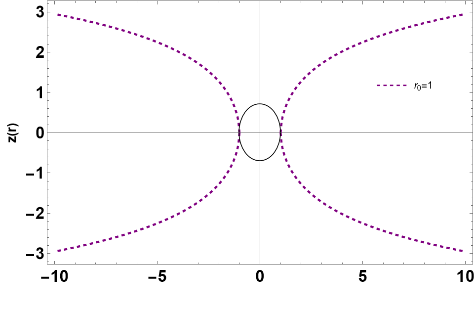
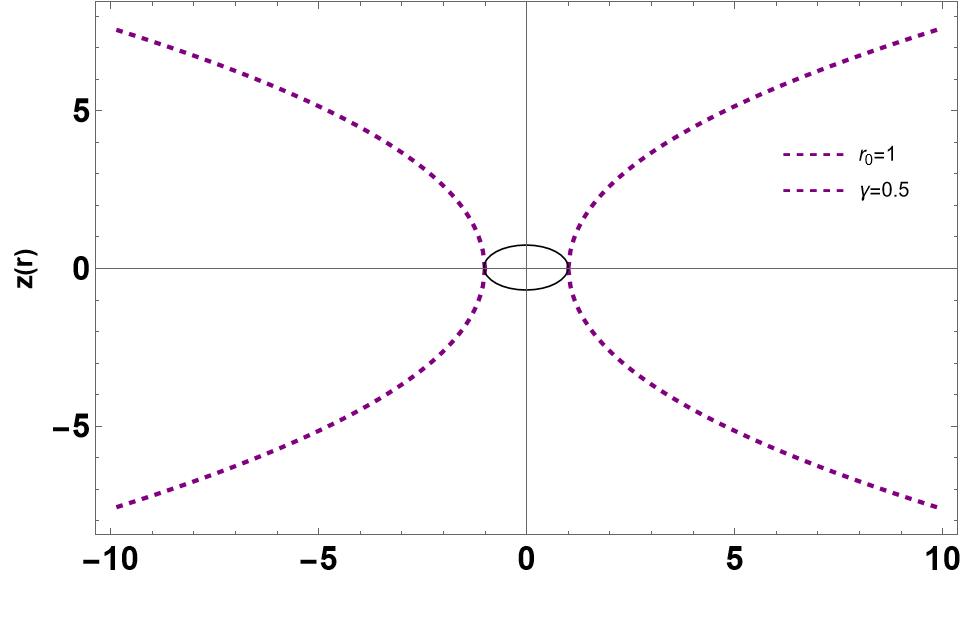
using the condition . Since, at the throat, we have . The imposes the restriction on for which . Moreover, we verify that as which confirms the asymptotic flatness. Using the Eq. (30), we plot the shape function for (dot-dashed), (dashed) and (solid) in the upper panel of Fig. 1, when .
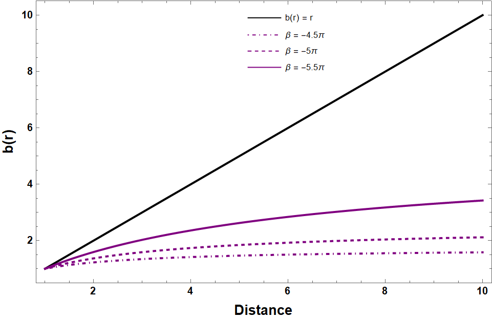
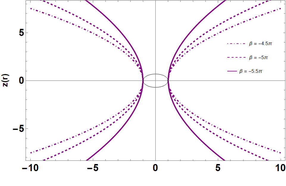
To get a better understanding about shape function, we find the equation for the embedding surface
| (31) |
In Fig. 1 (middle panel), we present the embedding diagram with Eqs. (30) and (31). The location of the WH throat is defined by the black ring, connects two distinct universes.
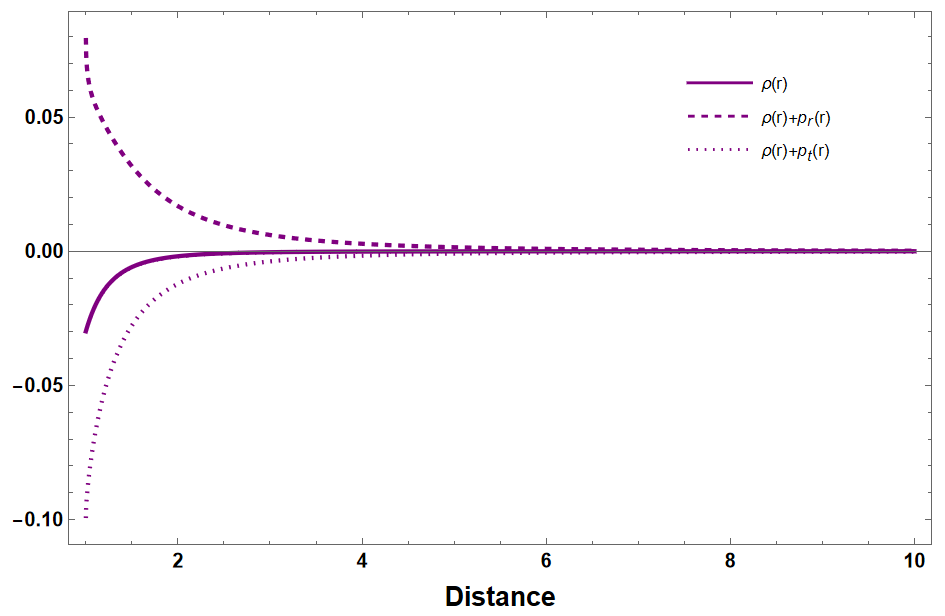
Using Eqs. (27)-(28) and Eq. (30) one finds the following relationships
| (32) | ||||
| (33) | ||||
| (34) |
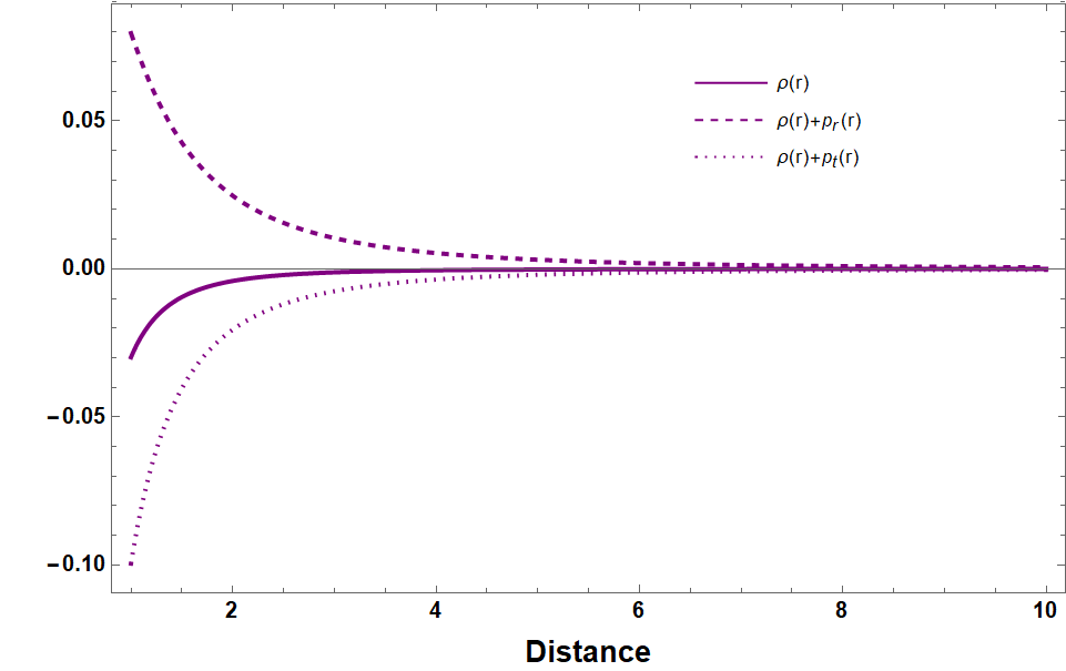
where . For , we plot (solid), (dashed) and (dotted) as functions of in the lower panel of Fig. 1. It is clear that both and tend to zero as . Clearly, for , energy density is negative outside the throat, while and . From Fig. 1 the NEC is violated outside the throat. The parameters of the solution are and , respectively.
At the throat, , one has
| (35) | |||
| (36) |
It is obvious that depending on the values of . In the region we have , and for . Moreover, we see that the situation is just reversed for the NEC along transverse direction (at the throat) i.e., . Note that equations are not-valid for . From these observations, we can infer that the model violates NEC throughout the spacetime and consequently the violation of WEC also.
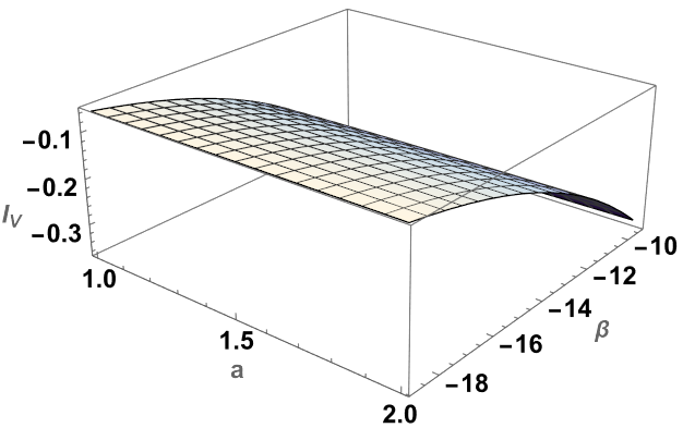
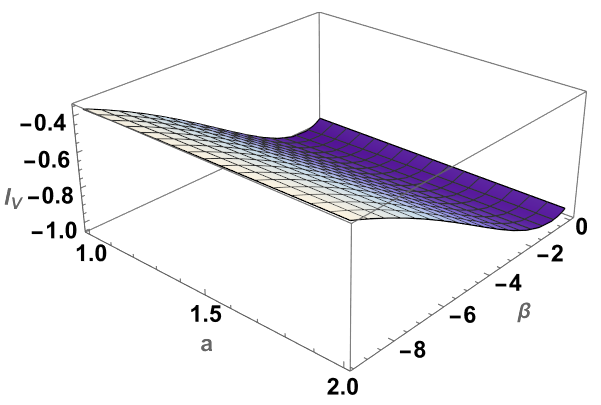
Here, we are also interested to quantify the total amount of exotic matter through “volume integral quantifier” (VIQ) [70]. This can be achieved through the definite integral (with a cut-off of the stress-energy at ):
| (37) |
and using the Eq. (33), we have
| (38) |
where we have defined , , , and , respectively. After carefully reviewing the Eq. (38), we can say that , when taking the limit . For more clarity, we plot Fig. 6, which depict that one can theoretically construct a traversable WH with small amount of NEC violating matter within the specified range of .
V.3 Solution for
Here, we consider a widely used specific form function given by . Notably a generalised version of this shape function appears in the work of Tripathy [67]. However, in that work the author commenced the study by referring to ‘tideless’ forces amounting to . Thereafter he adopted the classical Casimir force variation density going as where is the separation between two charged plates. Based on these he obtained the shape function above. In addition he was interested in quantum effects and the generalised uncertainty principle (GUP). Zubair et al [68] followed a similar approach to Tripathy however to fix the geometry of the models they assumed the existence of conformal Killing vectors. This places a restriction on the metric potentials, that is on the shape function profile. Our approach is quite different: We take the conventional understanding of vanishing tidal forces as and then we postulate forms of the shape function with the desired properties for a viable WH. In the upper panel of Fig. 3, we plot the embedding diagram using the shape function and Eq. (31).
Taking into account Eqs. (12)-(14) with the EoS (15), we have the following expressions
| (39) | |||
| (40) | |||
| (41) |
Solving the Eqs. (39)-(40), we get the expression for and in terms of and ,
| (42) | ||||
| (43) |
Using and into the Eq. (41), one obtains the following relationship
| (44) |
which may be integrated to yield the solution
where with and are integrating constants, which at the throat, reduce to
| (46) |
We need to impose the condition to ensure a regular solution. Thus, is finite at the throat. Moreover, we know that the range of is , and exists only when . Then the proposed range of for which is defined. If we consider the maximum value of then . Moreover, as . This gives a finite value, as the range of is finite. Finally, we arrive at a conclusion that given in Eq. (V.3) is finite as . So that this solution now reflects a traversable WH.
Considering the redshift function (V.3), one can rewrite the field equations (42)-(43) with substituting this into the Eq. (15),
| (47) | ||||
| (48) | ||||
| (49) |
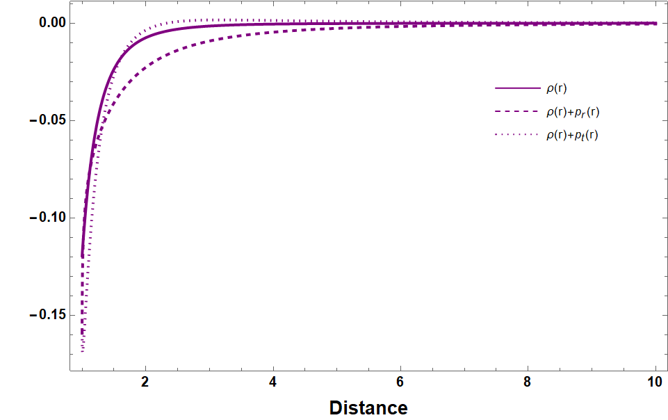
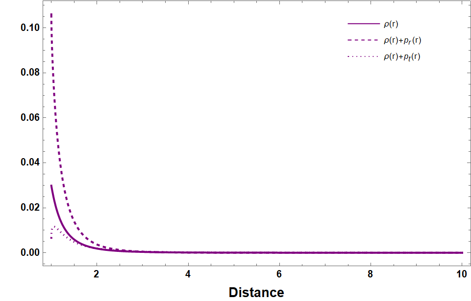
where and . In Fig. 3, we plot (solid), (dashed) and (dotted), respectively. For this case, we have plotted two different diagrams considering two different values of and , respectively. From the upper panel of Fig. 3, we see that the energy density, and two components for and are negative outside the throat i.e., . This means that the NEC is always violated outside the throat radius for . For configurations with , we find an interesting solution that the WEC (and also NEC) is satisfied, as can be seen from the lower panel of Fig. 3. Note that is not allowable range for WH construction, see the expression .
The NEC at the throat is given by
| (50) | ||||
| (51) |
It is clear that both when . Thus, the NEC is always violated for . On the other hand, we verify that that for . This would imply that , and are always positive when . As a closing remark we can say that realistic physical mechanisms such as the Casimir effect exist in order to support the geometry of traversable WHs. Exotic matter fields in the form of dark energy are therefore not compulsory. This is important as experimental support for dark energy is absent to date, whereas the Casimir phenomenon is a laboratory proven counter-intuitive effect.
To be precise, we consider VIQ to evaluate the total amount of exotic matter. Using the Eqs. (48) and (37), we are ready to give some comments on the amount of exotic matter. For complicated expression, we are not able to provide full analytical integration. Thus, we decide to perform an numerical integration for specific values of and with for small value of . Finally, we have
| (52) |
As a result, we clearly see that when . To make it easier, we plot Fig. 6 for the range of where we found that .
V.4 Solution for
Here, we consider the specific model for [69], where is of particularly interesting to have WH solutions satisfying the condition . In Fig. 5, where we have plotted the embedding diagram corresponding to the above mentioned shape function. Now, we take the field equations (12)-(14) with the EoS (15), which gives
| (53) | |||
| (54) | |||
| (55) |
where and . We take the field equations given in (53) and (54), and get the expression for and in terms of and ,
| (56) | |||
| (57) |
Using and into the Eq. (55), one obtains the following relationship
| (58) |
which may be integrated to yield the solution
| (59) |
where with and are integrating constants, which at the throat, reduce to
| (60) |
Let us point out a few considerations to maintain the regularity of the solution. We need to impose , so that is finite at the throat. Interestingly, we see that the considered case is almost similar to our previous case, and thus we are not discussing same analogy here in detail. Thus, we conclude that given in Eq. (59) is finite as , which permit to have a horizonless Solution.
Inserting the redshift function (59) into the expressions (56)-(57) with using this into the Eq. (15), we finally have
| (61) | ||||
| (62) | ||||
| (63) |
where . Having obtained the solutions for the matter fields, we plot (solid), (dashed) and (dotted) in Fig. 5. It is important to emphasize that the regions for the domain is where the WH is valid, see the expression . Note also that and is a point of discontinuity where the solution is not valid. Fig. 5 depicts the behaviour of the stress-energy components for and . Observing the figure, we see that and are negative, while for is positive outside the throat i.e., . This clearly indicate that the NEC is violation outside the throat radius within the specified region.
The NEC at the throat is given by
| (64) | ||||
| (65) |
In this case, we see that and when . On the other hand, and when . Thus, it is clear that the NEC is always violated.
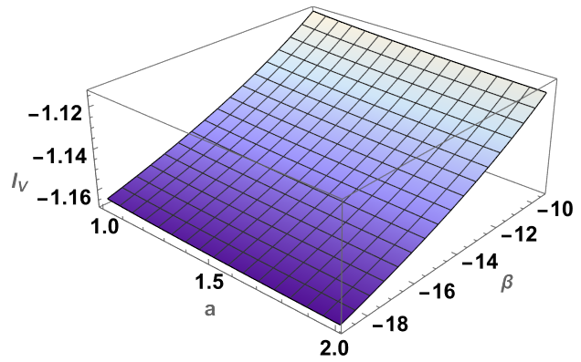
Finally, we determine the total amount of exotic matter through the VIQ. Thus, using the Eq. (37) and Eq. (66), we obtain an approximate analytical solutions for the definite integral with a cut-off of the stress-energy at :
| (66) | |||||
where and . For illustration we display in Fig. 6 for , and varying in domain is where the WH solution is valid. Observing Fig. 6 we can say that the amount of exotic matter can be reduced.
VI Concluding remarks
Invoking a Casimir type equation of state together with suitable shape and redshift functions, we presented complete analytical solutions for static and spherically symmetric asymptotically flat WH geometries in the background of theory. The novelty of our work lies in the use of this Casimir stress energy which is known to produce negative density and which is a necessity for the emergence of wormholes. The negative density causes a repulsive gravitational behaviour which sustains the opening of the WH throat. In contrast most treatments of wormholes rely on the negative density arising out of exotic fluids such as dark energy. The Casimir effect has the advantage that it is laboratory confirmed whereas dark energy is a speculative entity lacking empirical observational evidence to date. Invoking the Casimir behaviour in the study of WH geometry has attracted only limited attention historically. In our work we have adopted the approach of Kar and Sahadev [7] which, to the best of our knowledge has not been attempted before. A similar endeavour by Tripathi [67] utilised the quantum effects variation of density with plate-distance as well as considering the generalised uncertainty principle.
We have elected to study gravity which is a generalization of gravity such that the gravitational Lagrangian density depends on (Ricci scalar) and (stress-energy tensor). Part of the motivation of gravity is the coupling between geometry and matter, which has extensive applications in astrophysics and cosmology and the fact that this peculiar equation of state has not featured in the literature in theory.
In the geometrical representation, we have analyzed different energy conditions and investigated the effects of coupling constant on the WH structure. At the outset we show that a sustainable WH could not be possible for a thereby ruling out WHs with vanishing tidal forces. Subsequently by considering , we show that viable WH solutions exist provided that the coupling parameter is constrained as . In Fig. 1, we showed that the shape function in Eq. (30) satisfies all the necessary requirements, but the NEC is violated throughout the spacetime and consequently the violation of WEC also. This is welcome in WH geometry and physics. Finally, we consider as a form function and derive the stress energy tensor components. In this process the obtained redshift function in (V.3) is finite everywhere. This is a clear indication that spacetime has no event horizons. Moreover, we have shown that the WEC is satisfied throughout the entire spacetime by considering a negative value of coupling constant . This study shows that the Casimir stress energy is an ideal candidate for the study of wormholes and in future work we shall consider its effect in other modified gravitational field theories.
Acknowledgements.
In accordance with the visiting associateship scheme, A. Pradhan is grateful to IUCAA, Pune, India, for providing support and facilities. SH thanks the National Research Foundation of South Africa for support through Grant 138012.References
- [1] A.Einstein and N. Rosen. Phys. Rev., 48, 73, (1953).
- [2] M. S. Morris and K. S. Thorne, Am. J. Phys. 56, 395 (1988).
- [3] K. A. Bronnikov, Phil. Trans. A. Math. Phys. Eng. Sci. 380, 2222, (2022).
- [4] G. Dotti, J. Oliva and R. Troncoso, Phys. Rev. D 75, 024002 (2007).
- [5] M. Visser, Phys. Rev. D 39, 3182 (1989).
- [6] M. Visser, Nucl. Phys. B 328, 203 (1989).
- [7] S. Kar and D. Sahdev, Phys. Rev. D 52, 2030 (1995).
- [8] R. Garattini, Eur. Phys. J. C 79, 951 (2019).
- [9] M. Zubair, R. Saleem, Y. Ahmad, and G. Abbas International Journal of Geometric Methods in Modern Physics 16, 1950046 (2019).
- [10] J. Luis Rosa and P. M. Kull, Eur. Phys. J. C 82, 1154 (2022).
- [11] A. Banerjee, M. K. Jasim, S. G. Ghosh, Annals of Physics 433, 168575 (2021).
- [12] N.M. Garcia and F. S. N. Lobo, Modern Physics Letters A 26, 3067 (2011).
- [13] E. Papantonopoulos and C. Vlachos, Phys. Rev. D 101, 064025 (2020).
- [14] L. A. Anchordoqui, S. E. Perez Bergliaffa and D. F. Torres, Phys. Rev. D 55, 5226 (1997).
- [15] S. Bahamonde, M. Jamil, P. Pavlovic, and M. Sossich Phys. Rev. D 94, 044041 (2016).
- [16] M. Zubair, S. Waheed and Y. Ahmad Eur. Phys. J. C 76, 444 (2016).
- [17] T. Harko, F. S. N. Lobo, S. Nojiri and S. D. Odintsov, Phys. Rev. D 84, 024020 (2011).
- [18] S. Hansraj and A. Banerjee, Phys. Rev. D 97, 104020 (2018).
- [19] G. F. R. Ellis, H. van Elst, J. Murugan and J. P. Uzan, Class. Quant. Grav. 28, 225007 (2011).
- [20] G. F. R. Ellis, Gen. Rel. Grav. 46, 1619 (2014).
- [21] S. Hansraj, R. Goswami, G. Ellis and N. Mkhize, Phys. Rev. D 96, 044016 (2017).
- [22] P. Rastall, Phys. Rev. D 6, 3357 (1972).
- [23] P. Rastall, Can. J. Phys. 54, 66 (1976).
- [24] S. Hansraj, A. Banerjee and P. Channuie, Annals Phys. 400, 320 (2019).
- [25] S. Hansraj and A. Banerjee, Mod. Phys. Lett. A 35, 2050105 (2020).
- [26] J. Z. Yang, S. Shahidi and T. Harko, Eur. Phys. J. C 82, 1171 (2022).
- [27] H. Weyl, Space-Time-Matter (Dover Books on Physics), (1952).
- [28] E. Scholz, Einstein Stud. 14, 261 (2018).
- [29] P. A. M. Dirac, Proc. Roy. Soc. Lond. A 333, 403 (1973).
- [30] P. A. M. Dirac, Proc. R. Soc. Lond. A 338, 439 (1974).
- [31] N. Rosen, Foundations of Physics 12, 213 (1982).
- [32] M. Israelit, Gen. Rel. Grav. 43, 751 (2011).
- [33] M. Y. Piotrovich, S. V. Krasnikov, S. D. Buliga and T. M. Natsvlishvili, Mon. Not. Roy. Astron. Soc. 498, 3 (2020).
- [34] S. V. Sushkov, Phys. Rev. D 71, 043520 (2005).
- [35] F. S. N. Lobo, Phys. Rev. D 71, 084011 (2005).
- [36] F. S. N. Lobo, Phys. Rev. D 71, 124022 (2005).
- [37] M. Jamil, P. K. F. Kuhfittig, F. Rahaman and S. A. Rakib, Eur. Phys. J. C 67, 513 (2010).
- [38] M. Jamil and M. U. Farooq, Int. J. Theor. Phys. 49, 835 (2010).
- [39] M. Jamil, Eur. Phys. J. C 62, 609 (2009).
- [40] F. S. N. Lobo, F. Parsaei and N. Riazi, Phys. Rev. D 87, 084030 (2013).
- [41] M. Cataldo and F. Orellana, Phys. Rev. D 96, 064022 (2017).
- [42] F. Parsaei and S. Rastgoo, Phys. Rev. D 99, 104037 (2019).
- [43] P. K. F. Kuhfittig and V. D. Gladney, Adv. Stud. Theor. Phys. 12, 233 (2018).
- [44] M. Alcubierre and F. S. N. Lobo, Fundam. Theor. Phys. 189, 279 (2017).
- [45] M. Visser, Lorentzian Wormholes: From Einstein to Hawking, (American Institute of Physics, New York, 1995).
- [46] D. Wang and X.- h. Meng, Eur. Phys. J. C 76, 484 (2016).
- [47] P. Kanti, B. Kleihaus and J. Kunz, Phys. Rev. Lett. 107, 271101 (2011).
- [48] P. Kanti, B. Kleihaus and J. Kunz, Phys. Rev. D 85, 044007 (2012).
- [49] J. L. Blázquez-Salcedo, C. Knoll and E. Radu, Phys. Rev. Lett. 126, 101102 (2021).
- [50] R. A. Konoplya and A. Zhidenko, Phys. Rev. Lett. 128, 091104 (2022).
- [51] W. Israel, Nuovo Cim. B 44, 1 (1966).
- [52] M. Visser, S. Kar and N. Dadhich, Phys. Rev. Lett. 90, 201102 (2003).
- [53] F. S. N. Lobo, G. J. Olmo, E. Orazi, D. Rubiera-Garcia and A. Rustam, Phys. Rev. D 102, 104012 (2020).
- [54] P. Pavlovic and M. Sossich, Eur. Phys. J. C 75, 117 (2015).
- [55] T. Harko, F. S. N. Lobo, M. K. Mak and S. V. Sushkov, Phys. Rev. D 87, 06750 (2013).
- [56] A. De Benedictis and D. Horvat, Gen. Relativ. Gravit. 44, 2711 (2012).
- [57] M. Sharif and Z. Zahra, Astrophys. Space Sci. 348, 275 (2013).
- [58] E. F. Eiroa and G. Figueroa Aguirre, Eur. Phys. J. C 76, 132 (2016).
- [59] S. H. Mazharimousavi and M. Halilsoy, Mod. Phys. Lett. A 31, 1650192 (2016). A. Khaybullina and G. Tuleganova, Mod. Phys. Lett. A 34, 1950006 (2019).
- [60] N. Godani and G. C. Samanta, New Astron. 80, 101399 (2020).
- [61] O. Jose Barrientos and F. R. Guillermo, Phys. Rev. D 90, 028501 (2014).
- [62] D. Deb, S. V. Ketov, S. K. Maurya, M. Khlopov, P. H. R. S. Moraes and S. Ray, Mon. Not. Roy. Astron. Soc. 485,5652 (2019).
- [63] S. K. Maurya, A. Errehymy, D. Deb, F. Tello-Ortiz and M. Daoud, Phys. Rev. D 100, 044014 (2019).
- [64] S. Biswas, D. Shee, B. K. Guha and S. Ray, Eur. Phys. J. C 80, 175 (2020).
- [65] M. R. Mehdizadeh, M. Kord Zangeneh and F. S. N. Lobo, Phys. Rev. D 91, 084004 (2015).
- [66] M. R. Mehdizadeh and F. S. N. Lobo, Phys. Rev. D 93, 124014 (2016).
- [67] S. K. Tripathy, Phys. Dark Univ. 31, 100757 (2021).
- [68] M. Zubair, S. Waheed, M. Farooq, A. H. Alkhaldi and A. Ali, Eur. Phys. J. Plus 138, 902 (2023).
- [69] F. S. N. Lobo, Class. Quant. Grav. 25, 175006 (2008).
- [70] S. Kar, N. Dadhich and M. Visser, Pramana 63, 859 (2004).