Debiased Offline Representation Learning for Fast Online Adaptation in Non-stationary Dynamics

Abstract

Developing policies that can adjust to non-stationary environments is essential for real-world reinforcement learning applications. However, learning such adaptable policies in offline settings, with only a limited set of pre-collected trajectories, presents significant challenges. A key difficulty arises because the limited offline data makes it hard for the context encoder to differentiate between changes in the environment dynamics and shifts in the behavior policy, often leading to context misassociations. To address this issue, we introduce a novel approach called Debiased Offline Representation for fast online Adaptation (DORA). DORA incorporates an information bottleneck principle that maximizes mutual information between the dynamics encoding and the environmental data, while minimizing mutual information between the dynamics encoding and the actions of the behavior policy. We present a practical implementation of DORA, leveraging tractable bounds of the information bottleneck principle. Our experimental evaluation across six benchmark MuJoCo tasks with variable parameters demonstrates that DORA not only achieves a more precise dynamics encoding but also significantly outperforms existing baselines in terms of performance.

1 Introduction

In Reinforcement Learning (RL), the agent attempts to find an optimal policy that maximizes the cumulative reward obtained from the environment  (Sutton & Barto, 2018). However, online RL training typically requires millions of interaction steps (Kaiser et al., 2019), posing a risk to safety and cost constraints in real-world scenarios (Garcıa & Fernández, 2015). Different from online RL, offline RL (Fujimoto et al., 2019; Wu et al., 2019; Kumar et al., 2020; Ran et al., 2023) aims to learn an optimal policy, exclusively from datasets pre-collected by certain behavior policies, without further interactions with the environment. Showing great promise in turning datasets into powerful decision-making machines, offline RL has attracted wide attention recently (Levine et al., 2020b).

Previous offline RL methods commonly assume that the learned policy will be deployed to environments with stationary dynamics (Kumar et al., 2020), while unavoidable perturbations in real world will lead to non-stationary dynamics (Choi, 2000). For example, the friction coefficient of the ground changes frequently when a robotic vacuum walks on the floor covered by different surfaces. Policies trained for stationary dynamics will be unable to deal with non-stationary ones since the optimal behaviors depend on the certain dynamic. Nevertheless, training an adaptable policy from offline datasets for online adaptation in non-stationary dynamics is overlooked in current RL studies. In this paper, we focus on the setting where the environment dynamics, such as gravity or damping of the controlled robot, change unpredictably within an episode.

Offline Meta Reinforcement Learning (OMRL), which trains a generalizable meta policy from a multi-task dataset generated in different dynamics, offers a potential solution to handle non-stationary dynamics. Among existing OMRL methods, the gradient-based approaches (Lin et al., 2022b) may not be ideal solutions, as extra gradient updates are likely to cause drastic performance degradation due to the instability of policy gradient methods  (Haarnoja et al., 2018). In comparison, context-based OMRL methods (Yuan & Lu, 2022; Li et al., 2021) extract task-discriminative information from trajectories by learning a context encoder. However, these methods still face severe challenges when encountering non-stationary dynamics. Firstly, the representations from the learned encoder may exhibit a biased correlation with the data-collecting behavior policy (Yuan & Lu, 2022). As a consequence, it will fail to correctly identify the environment dynamics when the learned policy, instead of the behavior policy, is used to collect context during online adaptation. Secondly, existing OMRL methods generally require collecting short trajectories before evaluation during meta-testing phrase (Li et al., 2021), which is not allowed in non-stationary dynamics because the changes of dynamics are unknown to the agent.

To tackle the aforementioned issues, we propose DORA (abbreviation of Debiased Offline Representation learning for fast online Adaptation). DORA employs a context encoder that uses the most recent state-action pairs to infer the current dynamics. In order to learn a debiased task representation, we respectively derive a lower bound to maximize the mutual information between the dynamics encoding and environmental data, and an upper bound to minimize mutual information between the dynamics encoding and the actions of the behavior policy, following the Information Bottleneck (IB) principle. Specifically, the lower bound is derived to urge the encoder to capture the task-relevant information using InfoNCE (Oord et al., 2018). And the upper bound is for debiasing representations from behavior policy, formalized as the Kullback-Leibler (KL) divergence between the representations with and without behavior policy information of each timestep. The contextual policy is then trained by an offline RL algorithm, such as CQL (Kumar et al., 2020). Experiment results on six MuJoCo tasks with three different changing parameters demonstrate that DORA remarkably outperforms existing OMRL baselines. Additionally, we illustrate that the learned encoder can swiftly identify and adapt to frequent changes in environment dynamics. We summarize our main contributions as below:

• We propose an offline representation learning method for non-stationary dynamics, which enables fast adaptation to tasks with frequent dynamics changes.

• We derive a novel objective for offline meta learning, which trains the encoder to reduce the interference of the behavior policy to correctly identify dynamics.

• Experimentally, our method achieves better performance in unseen dynamics on-the-fly without pre-collecting trajectories, compared with baselines.

2 Preliminaries

Reinforcement Learning

We consider the infinite-horizon Markov Decision Process (MDP)  (Sutton & Barto, 2018), which can be formulated as a tuple $M=\langle\mathcal{S},\mathcal{A},P,r,d_{0},\gamma\rangle$. Here, $\mathcal{S}$ and $\mathcal{A}$ represent the state space and action space, respectively. Let $\Delta_{X}$ be the set of probability measures over any space $X$. We use $P:\mathcal{S}\times\mathcal{A}\to\Delta_{\mathcal{S}}$ to denote the environment transition function, or equivalently, dynamics. $r:\mathcal{S}\times\mathcal{A}\to\mathbb{R}$ is the reward function. $d_{0}$ denotes the distribution of initial states. $\gamma\in\left[0,1\right)$ is the discount factor. The discounted cumulative reward starting from time step $t$ is defined as $G_{t}=\sum_{k=0}^{\infty}\gamma^{k}r\left(s_{t+k},a_{t+k}\right)$, where $G_{0}$ is known as return. The policy $\pi:\mathcal{S}\to\Delta_{\mathcal{A}}$ specifies a distribution over the action space $\mathcal{A}$, given any state $s\in\mathcal{S}$. RL aims to find an optimal policy $\pi^{*}$ which maximizes the expected return $J_{M}(\pi)$, i.e., $\pi^{*}\in\arg\max_{\pi}J_{M}(\pi):=\mathbb{E}[G_{0}]$. When executing the policy $\pi(a|s)$ starting from $s_{t}$, the value function can be formulated as $V^{\pi}(s)=\mathbb{E}_{\pi}\left[G_{0}|s_{0}=s\right]$. Similarly, The action value function is $Q^{\pi}(s,a)=$ $\mathbb{E}_{\pi}\left[G_{0}\mid s_{0}=s,a_{0}=a\right]$.

Context-based OMRL

OMRL combines offline RL (Kumar et al., 2020) and meta RL (Rakelly et al., 2019), aiming to learn a meta policy from offline datasets collected from multiple tasks. The goal of OMRL is to learn a meta policy $\pi_{\theta}$ with $\theta$ denoting the learnable parameters, which can generalize to unseen tasks not appearing in the training dataset. The $N$ tasks for meta training $\mathcal{M}=\{M_{i}\}_{i=1}^{N}$ are sampled from the same task distribution $P_{\rm train}$. We assume that all tasks share the same state space and action space, with the only difference lying in dynamics. For each task $M_{i}$, we have an offline dataset $D_{i}$ of trajectories collected by an unknown behavior policy $\pi^{b}_{i}$. For simplicity, we may omit the subscript $i$. In this paper, we use $\tau_{0:H-1}=\{s_{0},a_{0},\ldots,s_{H-1},a_{H-1}\}$ to denote a short offline trajectory of length $H$ for dynamics identification. During OMRL training, the meta policy $\pi_{\theta}$ is trained on all the offline datasets. In the testing phase, the agent encounters unseen tasks over $P_{\rm test}$, and the meta policy needs to generalize to these tasks with limited interactions. As mentioned before, the objective of OMRL is to maximize the expected return in any testing tasks sampled from $P_{\rm test}$, i.e.,

$$\underset{\theta}{\max}\ J(\pi_{\theta}):=\mathbb{E}_{M\sim P_{\rm test}}\left[J_{M}\left(\pi_{\theta}\right)\right].$$ (1)

Context-based OMRL utilizes an encoder $p_{\phi}$, where $\phi$ is the learnable parameters, to output a $m$-dimensional task representation $z\in\mathbb{R}^{m}$. In experiments shown in Section 5, we set $m=2$. The task representation could be regarded as auxiliary information to help the offline policy $\pi_{\theta}$ to identify the current testing task. For clarity, we use $\pi_{\theta}(a|s,z)$, $V^{\pi}(s,z)$, $Q^{\pi}(s,a,z)$ thereafter to respectively denote the meta policy, meta value function and meta action value function taking the task representation $z$ as an additional input. Compared with the online context-based encoder, the offline-trained encoder is more susceptible to behavior policies due to the limited state and action space coverage of the datasets, which is detrimental in context-based OMRL.

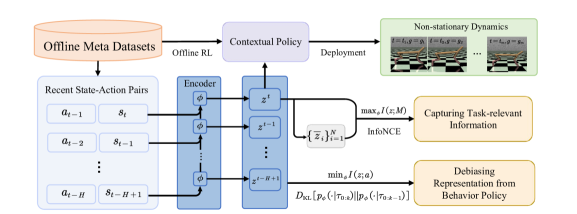
Figure 1: The DORA framework. The encoder utilizes recent state-action pairs to maintain a set of representations $\{z^{t-H+1},\cdots,z^{t}\}$ and $z^{t}$ updates the moving average task encodings $\{\bar{z}_{i}\}_{i=1}^{N}$. All these representations are then used to optimize the encoder. The contextual policy is trained through offline RL on the datasets, where each transition is labeled with its representation by the learned encoder.

Information Bottleneck

In information theory, the IB concept involves extracting essential information by constraining the information flow, thereby finding a delicate equilibrium between preserving target-related information and achieving efficient compression (Tishby et al., 2000). This problem can be framed as the minimization of mutual information $I$ between the source random variable $X$ and its representation $\hat{X}$ for efficient compression, alongside the maximization of mutual information between $\hat{X}$ and the target $Y$ to retain target-related information (Tishby & Zaslavsky, 2015). The pursuit of an optimal $\hat{X}$ is cast as the following maximization problem:

$$\text{max}_{\hat{X}}I(\hat{X};Y)-\beta I(X;\hat{X}).$$ (2)

Here, $I(\hat{X};Y)=\int\int p(\hat{x},y)\log\left(\frac{p(\hat{x},y)}{p(\hat{x})p(y)}\right)\,d\hat{x}\,dy$, where $p(\hat{x},y)$ is the joint probability density function of $(\hat{x},y)\in\hat{X}\times Y$, and $p(\hat{x})$ and $p(y)$ are marginal probability density functions of $\hat{x}\in\hat{X}$ and $y\in Y$, respectively. The hyper-parameter $\beta$ represents the tradeoff between compression and fitting. IB enables the context encoder to learn abstract and high-level representations, which helps to improve the generalization ability of the meta policy on unseen tasks (Sohn et al., 2015; Chen et al., 2018).

3 Method

In this section, we present the DORA framework, which learns a dynamics-sensitive trajectory encoder that mitigates biases from the behavior policy and effectively adapts to non-stationary dynamics. In Section 3.1, we adhere to the information bottleneck principle to formulate the objective for offline meta-encoder learning. Subsequently, in Section 3.2 and Section 3.3, we convert IB into two tractable losses. Section 3.4 elaborates on the proposed DORA framework (see Figure 1) including its implementation details.

3.1 From IB to Debiased Representations

Due to the fact that the offline dataset, generated by fixed behavior policies, exhibits limited coverage of the state and action space, the encoder tends to inaccurately treat the behavior policy as a prominent feature for task identification. Such a predicament can result in the decline of the performance of the contextual policy, given its dependency on the encoder’s responsiveness to shifts in environmental dynamics. Thus it is crucial for the encoder to discern tasks based on the dynamics rather than the behavior policy.

We follow the IB principle to tackle this issue. Specifically, our approach involves maximizing the mutual information between representations and tasks to encapsulate dynamics-relevant information, while simultaneously minimizing the mutual information between representations and actions of behavior policies to alleviate biases stemming from the behavior policy. Given a training task $M\sim P_{\rm train}$ and the offline trajectory $T$ collected on $M$ with trajectory length $H$, this idea can be formulated as:

$$\text{max}_{\phi}I(Z;M)-\beta I(Z;A),$$ (3)

where $Z\sim p_{\phi}(\cdot|T)$, $A\sim\pi^{b}(\cdot|s)$, $s\in\mathcal{S}$ being any state.

3.2 Contrastive Dynamics Representation Learning

The first term in Equation 3, $I(Z;M)$, is used for the learned representation to effectively encapsulate dynamics-relevant information. Since directly optimizing $I(Z;M)$ is intractable, we derive a lower bound of it as shown in Theorem 3.1, which formulates the problem of maximizing $I(Z;M)$ as a contrastive learning objective. By training the encoder to distinguish between positive and negative samples, the encoder acquires the capability to generate representations that correctly embed the dynamics information.

Theorem 3.1.

Denote a set of $N$ tasks as $\mathcal{M}$, in which each task $M_{i}$ is sampled from the same training task distribution $P_{\rm train}$. Let random variables $M\in\mathcal{M}$, $T$ be a trajectory collected in $M$, $Z\sim p_{\phi}(\cdot|T)$, $p(Z)$ is the prior distribution of $Z$, then we have

$$I(Z;M)\geq\mathbb{E}_{M,T,Z}\left[\log\frac{\frac{p_{\phi}\left(Z\mid T\right)}{p\left(Z\right)}}{\sum_{i=1}^{N}\frac{p_{\phi}\left(Z_{i}\mid T^{i}\right)}{p\left(Z_{i}\right)}}\right]+\log N,$$

where $T^{i}$ is a trajectory collected in task $M_{i}$, $Z_{i}\sim p_{\phi}(\cdot|T^{i})$, and $i\in\{1,2,\cdots,N\}$.

Due to space limitations, we defer the proof of Theorem 3.1 to Appendix A. In practice, to approximate $p_{\phi}(Z|T)/p(Z)$, we choose the radius basis function $S(z_{i},z_{j})=\mathrm{exp}(-||z_{i}-z_{j}||^{2}/{\alpha})$, which measures the similarity between the two representations $z_{i}$ and $z_{j}$ (Mnih & Teh, 2012). Here, $\alpha$ is a hyper-parameter. We then obtain the distortion loss $\mathcal{L}_{\text{Dist}}$ as follows:

$$\mathcal{L}_{\text{Dist}}(\phi)=-\sum_{\begin{subarray}{c}M_{i}\in\mathcal{M},\\ \tau^{i}\in D_{i}\end{subarray}}\left[\mathrm{log}\left(\frac{S\left(z_{i},\bar{z}_{i}\right)}{\sum_{j=1}^{N}S\left(z_{i},\bar{z}_{j}\right)}\right)\right],$$ (4)

where $z_{i}$ is encoded by the encoder $p_{\phi}$ from trajectory $\tau^{i}$. $\bar{z}_{i}$ denotes the average task representation for task $i$, updated by $\bar{z}_{i}\leftarrow\lambda z_{i}+(1-\lambda)\bar{z}_{i},$ where $\lambda\in(0,1)$ is a hyper-parameter. Intuitively, by grouping trajectories from the same task while distinguishing those from different tasks, the distortion loss will help the encoder to extract dynamics-relevant information.

3.3 Debiasing Representation from Behavior Policy

Ideally, the learned representation should be minimally influenced by the behavior policy. Hence, as shown in the second term in Equation 3, we minimize the mutual information $I(Z;A)$ between representations and actions of behavior policy. However, it is intractable to precisely calculate $I(Z;A)$. We thus consider deriving an upper bound of it. Firstly, we have the following theorem.

Theorem 3.2.

Given a training task $M\in\mathcal{M}$, a trajectory $T$ collected in $M$ and $Z\sim p_{\phi}(\cdot|T)$, we have

$$I(Z;A)\leqslant\mathbb{E}_{A}\left[\ D_{\mathrm{KL}}\left[p\left(\cdot\mid A\right)\|t(\cdot)\right]\right],$$ (5)

where $t(Z)$ is an arbitrary distribution over $\mathbb{R}^{m}$ and $D_{\rm KL}$ is the Kullback-Leibler divergence (Kullback & Leibler, 1951).

The proof of Theorem 3.2 is deferred to Appendix A. To convert Equation 5 into a tractable optimization objective, we choose $p_{\phi}(\cdot|\tau_{0:t-1})$ to be the distribution $t(Z)$ in practice. Surprisingly, we find that $p(\cdot|A)$ in Equation 5 can be cast to $p_{\phi}(\cdot|\tau_{0:t})$ since $a_{t-1}$ generated by $\pi^{b}(\cdot|s_{t-1})$ carries the information of the behavior policy and $s_{t}$, which is sampled from $P(\cdot|s_{t-1},a_{t-1})$, is independent of the behavior policy. We thus get the following debias loss $\mathcal{L}_{\rm Debias}$:

$$\mathcal{L}_{\rm Debias}(\phi)=\sum_{\begin{subarray}{c}M_{i}\in\mathcal{M},\\ \tau^{i}_{0:H}\in D_{i},\\ t\in\{1,2,\cdots,H\}\end{subarray}}D_{\mathrm{KL}}\left[p_{\phi}(\cdot|\tau^{i}_{0:t})\|p_{\phi}(\cdot|\tau^{i}_{0:t-1})\right],$$ (6)

For task $M_{i}$, we can get a trajectory segment $\tau_{0:H-1}$ with length $H$ given a full trajectory randomly sampled from $D_{i}$. If $s_{0}\in\tau_{0:H-1}$ is sampled from $d_{0}$, we use a zero vector with the same dimension of the action to be $a_{-1}$.

Algorithm 1 DORA Training

  Input: context encoder $p_{\phi}$, offline datasets $\{D_{i}\}_{i=1}^{N}$, short trajectory length $H$, batch size $U$, contextual policy $\pi_{\theta}$, contextual action function $Q_{\psi}$

   // Context Encoder Training

  for step = 1, 2, $\cdots$ do

     for $u=1$ to $U$ do

        Randomly sample a task $i\in\{1,2,\cdots,N\}$

        Sample a trajectory $\tau^{u}$ with length $H$ from $D_{i}$ randomly

     end for

     Let $\mathcal{B}_{1}=\{\tau^{u}\}_{u=1}^{U}$

     Infer representation $z_{u}$ from $\tau^{u}$ with $p_{\phi}$, $\forall\tau^{u}\in\mathcal{B}_{1}$

     Update the moving average task representation $\{\bar{z}_{i}\}_{i=1}^{N}$

     Get encoder loss $\mathcal{L}_{\mathrm{DORA}}(\phi)$ from Equation 7

     Update encoder $p_{\phi}$ with $\phi\leftarrow\phi-\alpha\nabla_{\phi}\mathcal{L}_{\mathrm{DORA}}(\phi)$

  end for

  // Policy Training

  for step = 1, 2, $\cdots$ do

     Randomly get a minibatch $\mathcal{B}_{2}=\{\tau^{u}\}_{u=1}^{U}$

     Infer representation $z_{u}$ from $\tau^{u}$ with $p_{\phi}$, $\forall\tau^{u}\in\mathcal{B}_{2}$

     Augment the states of minibatch $\mathcal{B}$ with $\{z_{u}\}_{u=1}^{U}$

     Update $\pi_{\theta}$ and $Q_{\psi}$ with CQL (Kumar et al., 2020) using $\{z_{u}\}_{u=1}^{U}$ on $\mathcal{B}_{2}$

  end for

3.4 A Practical Implementation

We take the Recurrent Neural Network (RNN) as the backbone of the encoder (Cho et al., 2014). The encoder receives a historical sequence of state-action pairs to generate the representation. By restricting the length of the RNN, we can adjust the amount of historical trajectory information retained in the encoder (Luo et al., 2022), which is helpful when the dynamic changes. Specifically, let $H$ be the history length, then the representation at step $t$ is denoted as $z_{i}^{t}\sim p_{\phi}(\cdot|\tau_{t-H:t})$, where $\tau_{t-H:t}=\{a_{t-H},\ldots,s_{t-1},a_{t-1},s_{t}\}$. If the history length is less than $H$, we will use the zero padding trick (Cho et al., 2014). The overall architecture is shown in Figure 1.

During the meta-training process, the encoder $p_{\phi}$ is updated using the the following loss:

$$\mathcal{L}_{\text{DORA}}(\phi)=\mathcal{L}_{\text{Dist}}(\phi)+\beta\mathcal{L}_{\text{Debias}}(\phi).$$ (7)

After the encoder is trained to convergence, we train the meta policy via CQL (Kumar et al., 2020). During meta-testing, the encoder infers the task representation $z$ based on the trajectories collected up to date. At each step, the current representation $z$ and state $s$ are together input into the meta policy, yielding a policy adapted to the current dynamics. Different from existing approaches (Yuan & Lu, 2022; Li et al., 2021), our approach does not require to pre-collect trajectories before policy evaluation, which achieves fast online adaptation on-the-fly. To sum up, the pseudocodes of meta training and meta testing are illustrated in Algorithm 1 and Algorithm 2, respectively.

4 Related Work

In this section, we introduce works related to our framework. Section 4.1 provides an overview of related works in offline RL. Section 4.2 shows how online RL methods handle non-stationary dynamics. Finally, Section 4.3 delves into the realm of OMRL, exploring relevant research and focusing on the challenges and strategies in this domain.

4.1 Offline RL

Offline RL learns policies from the dataset generated by certain behavior policies without online interaction with the environment, which helps avoid the safety concerns of online RL. The key challenge of offline RL lies in the distribution shift problem (Levine et al., 2020a), thus algorithms in this domain typically impose constraints on the training policy to keep it close to the behavior policy. Many model-free approaches (Fujimoto et al., 2019; Wu et al., 2019; Kumar et al., 2020; Ran et al., 2023) introduce regularization terms by considering the divergence between the learned policy and the behavior policy to constrain policy deviation. CQL (Kumar et al., 2020) directly learns a conservative state-action value function to alleviate the overestimation problem. Model-based methods (Yu et al., 2020; Kidambi et al., 2020; Yu et al., 2021) pre-train an environment model from the dataset, then use the model to generate out-of-dataset predictions for state-action transitions.

4.2 RL in Non-stationary Dynamics

To overcome the unavoidable perturbations in real world, recent years have seen an increasing number of research into RL in non-stationary dynamics, including continual RL and meta RL methods. Continual learning approaches aim to enable agents to continuously learn when faced with unseen tasks and avoid forgetting old tasks (Khetarpal et al., 2022). Policy consolidation (Kaplanis et al., 2019) integrates the policy network with a cascade of hidden networks and uses history to regularize the current policy to handle changing dynamics. The meta learning methods (Nagabandi et al., 2019), including the gradient-based methods and context-based methods, adapt to new tasks quickly by leveraging experience from training tasks. Specifically, the gradient-based meta RL methods (Finn et al., 2017) update the policy with gradients in the testing tasks, which are not suitable for non-stationary dynamics since real-world tasks may not allow for extra updates of the gradient. Context-based meta RL infers task-relevant information by learning a context encoder. In these methods, PEARL (Rakelly et al., 2019) employs variational inference to learn a context encoder. ESCP (Luo et al., 2022) utilizes an RNN-based context encoder to rapidly perceive changes in dynamics, enabling fast adaptation to new environments.

However, both continual RL and online context-based RL methods require online interactions, which are infeasible in the offline setting. As far as we know, there is currently no method capable of learning an effective adaptive policy in non-stationary dynamics in the paradigm of offline RL.

Table 1: Performance on the MuJoCo tasks in stationary dynamics. Top: Average normalized return $\pm$ standard deviation over 5 random seeds in testing tasks with IID dynamics. Bottom: Average normalized return $\pm$ standard deviation over 5 random seeds in testing tasks with OOD dynamics.

Environment	Offline ESCP	FOCAL	CORRO	Prompt-DT	DORA (Ours)
Cheetah-gravity	78.22 $\pm$ 21.13	51.99 $\pm$ 10.44	56.70 $\pm$ 15.48	49.59 $\pm$ 18.44	86.31 $\pm$ 16.45
Pendulum-gravity	96.55 $\pm$ 17.24	74.95 $\pm$ 12.55	76.82 $\pm$ 11.39	34.71 $\pm$ 15.95	100.08 $\pm$    0.01
Walker-gravity	52.82 $\pm$ 21.01	17.22 $\pm$ 12.05	44.49 $\pm$ 24.67	26.09 $\pm$    4.38	66.87 $\pm$ 21.64
Hopper-gravity	78.70 $\pm$ 19.17	34.10 $\pm$ 11.12	76.73 $\pm$ 14.19	42.44 $\pm$ 22.19	74.68 $\pm$ 17.34
Cheetah-dof	93.90 $\pm$ 24.49	39.36 $\pm$    9.27	53.80 $\pm$ 13.90	43.99 $\pm$ 16.23	97.85 $\pm$ 12.30
Cheetah-torso	56.21 $\pm$ 12.37	39.35 $\pm$    6.33	51.93 $\pm$ 16.22	45.30 $\pm$    5.60	61.60 $\pm$    1.19

Environment	Offline ESCP	FOCAL	CORRO	Prompt-DT	DORA (Ours)
Cheetah-gravity	64.30 $\pm$ 24.69	42.84 $\pm$ 12.14	38.72 $\pm$ 14.78	30.19 $\pm$    7.74	70.05 $\pm$ 17.02
Pendulum-gravity	86.02 $\pm$ 12.26	29.53 $\pm$ 14.41	57.21 $\pm$ 18.36	20.89 $\pm$ 10.99	98.09 $\pm$ 13.95
Walker-gravity	35.64 $\pm$ 20.12	12.69 $\pm$    7.08	29.02 $\pm$ 19.60	18.91 $\pm$ 11.78	43.33 $\pm$ 14.21
Hopper-gravity	71.96 $\pm$ 24.40	12.96 $\pm$    4.63	16.70 $\pm$    7.73	33.52 $\pm$ 10.82	71.52 $\pm$ 21.37
Cheetah-dof	73.60 $\pm$ 22.73	27.36 $\pm$ 12.27	43.08 $\pm$ 16.09	30.77 $\pm$ 10.46	77.48 $\pm$ 12.25
Cheetah-torso	56.50 $\pm$ 11.65	38.13 $\pm$    6.50	50.89 $\pm$    6.69	34.04 $\pm$    4.83	61.57 $\pm$    1.34

Table 2: Average normalized return $\pm$ standard deviation on the MuJoCo tasks in non-stationary dynamics over 5 random seeds.

Environment	Offline ESCP	FOCAL	CORRO	Prompt-DT	DORA (Ours)
Cheetah-gravity	65.42 $\pm$    6.54	49.96 $\pm$    6.41	54.08 $\pm$    8.54	23.52 $\pm$    7.75	71.61 $\pm$    7.56
Pendulum-gravity	85.92 $\pm$ 16.37	8.66 $\pm$    5.42	69.66 $\pm$ 14.80	11.36 $\pm$    5.86	97.11 $\pm$ 16.91
Walker-gravity	27.34 $\pm$ 10.75	17.91 $\pm$ 10.76	33.62 $\pm$ 14.86	14.49 $\pm$    2.81	40.46 $\pm$ 19.04
Hopper-gravity	54.29 $\pm$ 25.39	21.09 $\pm$    7.99	53.26 $\pm$ 20.36	15.91 $\pm$ 10.13	49.74 $\pm$ 23.74
Cheetah-dof	80.72 $\pm$    8.49	37.27 $\pm$ 13.76	52.41 $\pm$ 13.99	20.24 $\pm$ 12.66	91.83 $\pm$ 10.57
Cheetah-torso	53.99 $\pm$ 16.09	42.23 $\pm$ 15.01	45.58 $\pm$ 15.98	33.79 $\pm$ 10.51	60.13 $\pm$ 13.65

4.3 OMRL

OMRL extends meta RL to the paradigm of offline setting, aiming to generalize from experience of training tasks and facilitate efficient adaptation to unseen testing tasks. Gradient-based OMRL methods (Lin et al., 2022b) require a few interactions to adapt to unseen tasks, but the costly online gradient updates may not be allowed in the real world. In comparison, the context-based OMRL methods employ a context encoder for task inference, showing potential for faster adaptation. FOCAL (Li et al., 2021) uses distance metric learning loss to distinguish different tasks. Recently, the transformer-based approaches (Xu et al., 2022; Lin et al., 2022a) leverage Transformer networks for autoregressive training on blended offline data from multiple tasks, and construct policy by planning or setting return-to-go. As mentioned in our work, another key challenge for OMRL is that the encoder is required to accurately identify environment dynamics while debiasing representations from behavior policy. To alleviate this problem, CORRO (Yuan & Lu, 2022) employs contrastive learning to train context encoders and trains dynamic models to generate new samples. Nonetheless, these works still suffer from the entanglement of task dynamics and behavior policy experimentally. Besides, existing works need to pre-collect trajectories before evaluation in meta-testing phase (Gao et al., 2023; Zhou et al., 2023), which are not able to handle changing dynamics since the changes are unknown to the agent. From the information bottleneck perspective, we tackle these problems by developing a novel model-free framework that efficiently debiases the representations from the behavior policy and swiftly adapts to non-stationary dynamics.

5 Experiments

In this section, we conduct the experiments to answer the following questions:

• How does the learned encoder and contextual policy of DORA perform in unseen tasks of in-distribution (IID) and out-of-distribution (OOD) dynamics?

• How well does DORA identify and adapt to online non-stationary dynamics?

• Are the learned representations of DORA debiased from the behavior policy?

In Section 5.1, we introduce the environments and baselines. In Section 5.2, we compare the performance of different algorithms in IID, OOD, and non-stationary dynamics. In Section 5.3 and Section 5.4, we visualize the representations in IID dynamics and study the encoder’s sensitivity to non-stationary dynamics. In Section 5.5, we study whether the learned representations are debiased from behavior policy. In Section 5.6, we ablate multiple design choices in the encoder training process.

5.1 Environments and Baselines

Task Description. We choose MuJoCo tasks for experiments, including HalfCheetah-v3, Walker2d-v3, Hopper-v3, and InvertedDoublePendulum-v2, which are common benchmarks in offline RL (Todorov et al., 2012).

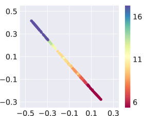
(a) DORA

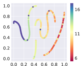
(b) FOCAL

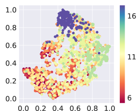
(c) CORRO

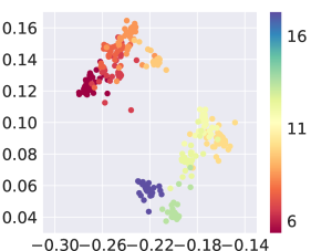
(d) Offline ESCP

Figure 2: Representation visualization in Cheetah-gravity tasks with IID dynamics. The points are the (projected) representations in a 2D latent space, with the color indicating the real parameters of dynamics.

Changing Dynamics. In order to generate different non-stationary dynamics, we change the physical parameters of the environments, namely gravity, dof-damping, and torso-mass. In IID dynamics, the parameter is uniformly sampled from the same distribution used for sampling training tasks. In OOD dynamics, the parameter is uniformly sampled from a distribution of the 20% range outside the IID dynamics. The parameter of non-stationary dynamics is sampled from the union of IID and OOD dynamics and changes every 50 timesteps. For convenience, we will abbreviate the experimental tasks as Cheetah-gravity, Pendulum-gravity, Walker-gravity, Hopper- gravity, Cheetah-dof, and Cheetah-torso.

Offline Data Collection. For each training dataset, we use SAC(Haarnoja et al., 2018) to train a policy for each training task independently to make sure the behavior policies are different in every single-task dataset. The offline dataset is then collected from the replay buffer. We gather 200,000 transitions for each single-task dataset, except for the tasks of Pendulum-gravity, which comprises 40,000 transitions.

Baselines: We compare DORA with 4 baselines. CORRO (Yuan & Lu, 2022), FOCAL (Li et al., 2021), and Prompt-DT (Xu et al., 2022) are prominent OMRL baselines in recent years. ESCP (Luo et al., 2022) is an online meta RL approach that effectively adapts to sudden changes. In order to operate this algorithm in the offline setting, we develop the offline ESCP as a baseline.

For all baselines and our method, a history trajectory of length $8$ is used to infer task representations. The debiased loss weight $\beta$ of our method is adjusted for different tasks. More details about the environments, offline datasets, and baselines in our experiments can be found in Appendix C.

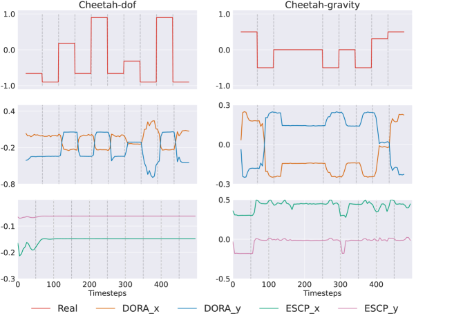
Figure 3: Representation tracking in a single trajectory in non-stationary dynamics. Real represents the normalized real parameters of unseen dynamics, DORA_x and DORA_y are the coordinates of the DORA’s representations in the 2D latent space, and the same applies to offline ESCP. Left: In Cheetah-dof. Right: In Cheetah-gravity.

5.2 Performance

We conduct experiments in IID, OOD, and non-stationary dynamics to compare the normalized return of the meta CQL policies learned with encoders from different algorithms. During testing, all algorithms are not permitted to pre-collect trajectories on new tasks, which means the encoder has to use short history trajectories generated by contextual policy to infer representations. As shown in Table 1, DORA outperforms the baselines in 5 of the total 6 MuJoCo tasks in both IID and OOD dynamics. Although offline ESCP performs better in Hopper-gravity, its performance suffers from a significant drop of 8.6% from IID to OOD tests, while the drop of DORA is 4.2%. The poor performance of Prompt-DT reveals that the transformer struggles to unleash its fitting and generalization capabilities in the absence of a well-defined prompt. DORA also excels at handling non-stationary dynamics, and its lead in most of the non-stationary environments is stronger than that in stationary environments, as illustrated in Table 2. These results suggest that DORA is effective in dealing with unseen non-stationary dynamics. As all baselines share the same contextual policies, it can thus be inferred that our encoder is more sensitive to the environment dynamics.

5.3 Representations in IID Dynamics

In this section, we compare the latent representations of DORA with other context-based OMRL baselines in Cheetah-gravity with IID dynamics, which are visualized in Figure 2. The representations of DORA and offline ESCP are encoded into two-dimensional vectors, while the representations of CORRO and FOCAL are encoded into higher dimensions and projected into 2D space via t-SNE (Van der Maaten & Hinton, 2008), following the approach used in the original paper.

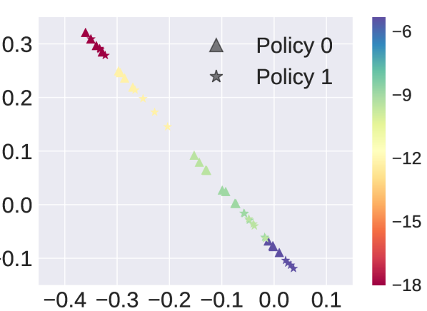
(a) Cheetah-gravity

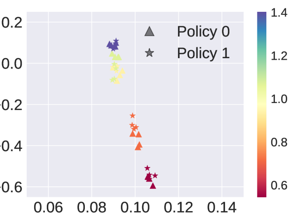
(b) Cheetah-dof

Figure 4: Visualization on task representations generated with 2 different context-collection policies in 5 unseen dynamics. Points of different shapes represent different policies. Left: In Cheetah-gravity. Right: In Cheetah-dof.

For each algorithm, we sample 200 short trajectories from the tasks with IID dynamics. The color of the encodings represents the real value of the changing dynamics parameter, and the color bar is on the right of each sub-figure correspondingly. The visualization results suggest that DORA’s representations appear as a straight line with parameters of dynamics gradually increasing or decreasing from one end to the other. In contrast, representations of CORRO and FOCAL are much more cluttered. Notably, although ESCP extracts linear-shape representations in the online setting, the offline ESCP fails to achieve the same effect. The shape of representations indicates that DORA’s encoder extracts more informative encodings and distinguishes the dynamics better than other baselines. We also visualize the encodings in OOD dynamics in Appendix D, which indicates DORA’s representations can be extended to unseen OOD dynamics.

5.4 Representation Tracking in Changing Dynamics

In order to study the encoder’s sensitivity to changing dynamics, we track the changes of representations during the adaptation in part of a single trajectory, which is shown in Figure 3. Real represents the normalized real parameters of unseen dynamics, x and y are the coordinates of the representations in the two-dimensional latent space. The environment dynamics change every 50 timesteps. It is evident to find that DORA’s encoding promptly follows almost every sudden change of dynamics, while offline ESCP generates few responses. As illustrated by these experimental results, DORA’s encoder infers robust representations and responds to non-stationary dynamics swiftly and precisely.

5.5 Debiased Representation Visualization

In this part, we study whether the learned representations are debiased from behavior policy. We first randomly choose the datasets of training tasks and train a Behavior Clone (BC, Ross & Bagnell (2010)) policy using each chosen dataset. Then these trained BC policies are used to roll out trajectories of $H$ timesteps in different unseen IID and OOD dynamics. Subsequently, we adopt DORA’s encoder to generate representations with these short trajectories, which are visualized in Figure 4.

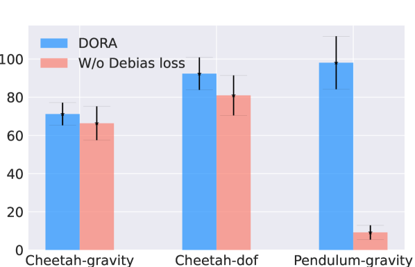
(a) Ablation on debias loss

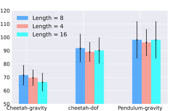
(b) Ablation on history length

Figure 5: Ablation studies: Average normalized return of DORA on 3 environments over 5 random seeds. The error bar stands for the standard deviation. Left: DORA with and without the debias loss. Right: RNN history lengths of 4, 8, and 16.

The experimental results show that representations inferred from trajectories generated by different policies still cluster together in the same task dynamics. Moreover, in comparison with the results of DORA in Figure 2, these representations are encoded to similar coordinates according to the real parameter of dynamics. These results powerfully demonstrate that DORA learns a dynamic-sensitive encoder, which takes the environment dynamics rather than behavior policy as a feature to generate debiased representations.

5.6 Ablation Studies

We first conduct ablation experiments to study the interdependence of the distortion loss and the debias loss. In Figure 5(a), the ablation experiments in 3 randomly chosen environments show that the debias loss significantly improves DORA. Notably, DORA can not converge without the distortion loss, so this ablated version is not included in the bar chart. Besides, to assess the impact of RNN history length on DORA’s performance, we compared instances with RNN lengths of 4, 8, and 16. The experimental results in Figure 5(b) demonstrate that DORA is not sensitive to the RNN history length. Additionally, we conducted sensitivity tests on the hyper-parameter $\beta$ in Section F.2.

6 Summary

In this paper, we consider the online adaptation issue in non-stationary dynamics from a fully offline perspective. We propose a novel offline representation learning framework DORA, in which the context encoder can efficiently identify changes in task dynamics and the meta policy is capable of rapidly adapting to online non-stationary dynamics. We follow the information bottleneck principle to formalize the offline representation learning problem. To conquer this problem, we derive a lower bound for the encoder to capture task-relevant information and an upper bound to debias the representation from behavior policy. We compare DORA with other OMRL baselines in environments of IID, OOD, and non-stationary dynamics. Experimental results show that DORA debiases the representation from behavior policy and exhibits better performance compared with baselines.

Appendix A Proofs

See 3.1

Proof.

We follow the proof of Yuan & Lu (2022).

$$I(Z;M) =\mathbb{E}_{M,Z}\left[\log\frac{p(Z\mid M)}{p(Z)}\right]$$

$$\overset{(a)}{=}\mathbb{E}_{M,Z}\left[\log\mathbb{E}_{T}\left[\frac{p_{\phi}(Z\mid T)}{p(Z)}\right]\right]$$

$$\geq\mathbb{E}_{M,Z}\mathbb{E}_{T}\left[\log\frac{p_{\phi}(Z\mid T)}{p(Z)}\right]$$

$$=\mathbb{E}_{M,T,Z}\left[\log\frac{p_{\phi}(Z\mid T)}{p(Z)}\right]$$

$$=-\mathbb{E}_{M,T,Z}\left[\log\left(\frac{p\left(Z\right)}{p_{\phi}\left(Z\mid T\right)}N\right)\right]+\mathrm{log}N$$

$$\geq-\mathbb{E}_{M,T,Z}\left[\log\left(1+\frac{p\left(Z\right)}{p_{\phi}\left(Z\mid T\right)}(N-1)\right)\right]+\mathrm{log}N$$

$$\geq-\mathbb{E}_{M,T,Z}\left[\log\left(1+\frac{p\left(Z\right)}{p_{\phi}\left(Z\mid T\right)}(N-1)\underset{M_{i}\in\mathcal{M}\backslash\{M\}}{\mathbb{E}}\frac{p_{\phi}\left(Z_{i}\mid T^{i}\right)}{p\left(Z_{i}\right)}\right)\right]+\mathrm{log}N$$

$$=-\mathbb{E}_{M,T,Z}\left[\log\left(1+\frac{p\left(Z\right)}{p_{\phi}\left(Z\mid T\right)}\sum_{M_{i}\in\mathcal{M}\backslash\{M\}}\frac{p_{\phi}\left(Z_{i}\mid T^{i}\right)}{p\left(Z_{i}\right)}\right)\right]+\mathrm{log}N$$

$$=\mathbb{E}_{M,T,Z}\left[\log\left(\frac{\frac{p_{\phi}\left(Z\mid T\right)}{p\left(Z\right)}}{\frac{p_{\phi}\left(Z\mid T\right)}{p\left(Z\right)}+\sum_{M_{i}\in\mathcal{M}\backslash\{M\}}\frac{p_{\phi}\left(Z_{i}\mid T^{i}\right)}{p\left(Z_{i}\right)}}\right)\right]+\mathrm{log}N$$

$$=\mathbb{E}_{M,T,Z}\left[\log\left(\frac{\frac{p_{\phi}\left(Z\mid T\right)}{p\left(Z\right)}}{\sum_{i=1}^{N}\frac{p_{\phi}\left(Z_{i}\mid T^{i}\right)}{p\left(Z_{i}\right)}}\right)\right]+\mathrm{log}N.$$

Here, $(a)$ is derived from the following expression:

$$\begin{split}\frac{p(Z\mid M)}{p(Z)}=\int\frac{p(\tau\mid M)p(Z\mid\tau,M)}{p(Z)}{\rm d}\tau=\int\frac{p(\tau)p_{\phi}(Z\mid\tau)}{p(Z)}{\rm d}\tau=\mathbb{E}_{T}\left[\frac{p_{\phi}(Z\mid T)}{p(Z)}\right].\end{split}$$

$\mathcal{M}\backslash\{M\}$ is a set of tasks in $\mathcal{M}$ except the task $M$. Thus, the proof is completed. ∎

See 3.2

Proof.

$$I(Z;A) =\int\int p\left(z,a\right)\log\frac{p\left(z\mid a\right)}{p(z)}{\rm d}z{\rm d}a$$

$$=\int\int p\left(z,a\right)\log p\left(z\mid a\right){\rm d}z{\rm d}a-\int p(z)\log p(z){\rm d}z$$

$$\overset{(b)}{\leqslant}\int\int p\left(z,a\right)\log p\left(z\mid a\right){\rm d}z{\rm d}a-\int p(z)\log t(z){\rm d}z$$

$$=\int\int p\left(a\right)p\left(z\mid a\right)\log\frac{p\left(z\mid a\right)}{t(z)}{\rm d}z{\rm d}a$$

$$=\mathbb{E}_{A}\left[\int p\left(z\mid A\right)\log\frac{p\left(z\mid A\right)}{t(z)}{\rm d}z\right]$$

$$=\mathbb{E}_{A}\left[D_{\rm KL}\left[p\left(\cdot\mid A\right)\|t(\cdot)\right]\right].$$

The inequality at $(b)$ is derived from $D_{\rm KL}\left[p(\cdot)\|t(\cdot)\right]\geq 0$. ∎

Appendix B DORA Testing

Algorithm 2 DORA Test

  Input: testing tasks $\{M_{i}^{\mathrm{test}}\}_{i=1}^{N}$, pre-trained context encoder $p_{\phi}$, pre-trained contextual policy $\pi_{\theta}(s,z)$, episode length $T_{s}$

  for each task $M_{i}\in\{M_{i}^{\mathrm{test}}\}_{i=1}^{N}$ do

     Initialize a history trajectory $\tau$ of length $H$ with zeros

     Get init state $s$ of $M_{i}$, append $(s,0)$ to $\tau$

     for $t\leq T_{s}$ do

        Infer $z$ from $\tau$ with $p_{\phi}$

        Get action $a=\pi_{\theta}(s,z)$

        Step in env and get the next state $s^{\prime}$

        $s\leftarrow s^{\prime}$

        Append $(s,a)$ to $\tau$

     end for

  end for

Appendix C Experiments Details

C.1 Task Description

We choose several MuJoCo tasks for experiments, including HalfCheetah-v3, Walker2d-v3, Hopper-v3, and InvertedDoublePendulum-v2, which are common benchmarks in offline RL (Todorov et al., 2012). In HalfCheetah, Walker2d, and Hopper, agents with several degrees of freedom need to learn to move forward as fast as possible. InvertedDoublePendulum originates from the classical control problem Cartpole, in which the agent needs to push the cart left and right to balance the pole on top of the bottom pole.

C.2 Environment Details

In this section, we provide detailed information about the dynamic-changing environments.

Gravity: Gravity is a global parameter in MuJoCo, which mainly affects the agent’s fall speed and vertical pressure. The dynamic is sampled by multiplying the default gravity $g_{0}$ with $1.5^{\mu},\mu\sim U[-a,a]$, where $a=1.5,1.8$ for IID and non-stationary dynamics, respectively. We uniformly sample $\mu$ from $U[-1.8,-1.5]\cup[1.5,1.8]$ for OOD dynamics.

Dof-Damping: Dof-damping refers to the damping value matrix applied to all degrees of freedom of the agent, serving as linear resistance proportional to velocity. The dynamics are sampled by multiplying the default damping matrix $A_{0}$ with $1.5^{\mu},\mu\sim U[-a,a]$, where $a=1.5,1.8$ for IID and non-stationary dynamics, respectively. We uniformly sample $\mu$ from $U[-1.8,-1.5]\cup[1.5,1.8]$ for OOD dynamics.

Torso-mass: Torsoz-mass is the mass of the agent’s torso. The dynamic is sampled by multiplying the default mass of torso $m_{0}$ with $1.5^{\mu},\mu\sim U[-a,a]$, where $a=1.5,1.8$ for IID and non-stationary dynamics, respectively. We uniformly sample $\mu$ from $U[-1.8,-1.5]\cup[1.5,1.8]$ for OOD dynamics.

Besides, each environment contains 10 tasks for training and 10 tasks for testing for both IID, OOD, and Non-stationary dynamics.

C.3 Details of the Offline Dataset

Maximum and Minimum Returns of Offline Datasets. In Table 3, we explicitly provide the maximum and minimum returns of offline datasets, which are used to calculate the normalized return in the policy evaluation. Specifically, the evaluation return $x$ for a particular is normalized using the formula $\frac{x-x_{\mathrm{min}}}{x_{\mathrm{max}}-x_{\mathrm{min}}}\times 100$, where $x_{\mathrm{max}}$ and $x_{\mathrm{min}}$ denote the corresponding maximum and minimum returns of each dataset.

Table 3: Maximum and minimum returns of offline datasets.

	Cheetah-gravity	Cheetah-dof	Cheetah-torso_mass	Hopper-gravity	Walker-graavity	Pendulum-gravity
Maximum	9218.48	8703.55	10060.59	3536.97	4630.10	9351.94
Minimal	-460.33	-613.09	-479.86	-1.22	-110.50	26.71

C.4 Introduction of Baselines

We compare DORA with 4 baselines which are listed below.

CORRO. CORRO (Yuan & Lu, 2022) designs a bi-level task encoder where the transition encoder is optimized by contrastive task learning and the aggregator encoder gathers all representations. CORRO uses Generative Modeling and Reward Randomization to generate negative pairs for contrastive learning. In our setting, the reward function remains the same across tasks thus we adopt the approach of Generative Modeling to compare.

FOCAL. FOCAL (Li et al., 2021) uses distance metric loss to learn a deterministic contextual encoder, which is also under the paradigm of contrastive learning. Additionally, FOCAL combines BRAC (Wu et al., 2019) to constrain the bootstrapping error.

Prompt-DT. Prompt-DT (Xu et al., 2022) employs the Transformer to tackle OMRL tasks. It utilizes a short segment of task trajectory containing task-specific information as the prompt input, guiding the transformer to model trajectories from different tasks. For each task dataset, we select the top 5 trajectories with the highest cumulative rewards to construct the task prompt. The remaining trajectories are then used for training.

Offline ESCP. ESCP (Luo et al., 2022) is an online meta RL approach that proposes variance minimization and Relational Matrix Determinant Maximization in optimizing the encoder to adapt to environment sudden changes. In order to fairly compare ESCP with other algorithms in offline settings, we develop an offline version of ESCP, denoted as offline ESCP. In this variant, we modify the online interaction process with the environment to sample trajectories from the offline dataset.

C.5 Configurations

The details of the important configurations and hyper-parameters used to produce the experimental results in this paper are listed in Table 4. Regarding the encoder model, we utilized a linear layer with 128 hidden units, a GRU network with 64 hidden units, and a linear layer with 64 hidden units for parameterization. The encoder’s output is scaled using a $\mathrm{Tanh}$ function.

Table 4: Configurations and hyper-parameters used in offline encoder training.

Configurations	Cheetah-gravity	Cheetah-dof	Cheetah-torso	Hopper-gravity	Walker-gravity	Pendulum-gravity
Debias loss weight	0.2	1.0	1.0	0.2	1.0	1.0
Distortion loss weight	1.0	1.0	1.0	1.0	1.0	1.0
History length	8	8	8	8	8	8
Latent space dim	2	2	2	2	2	2
Batch size	256	256	256	256	256	256
Learning rate	3e-4	3e-4	3e-4	3e-4	3e-4	3e-4
Training steps	2000000	2000000	2000000	2000000	2000000	400000

Appendix D Representation Visualization of DORA

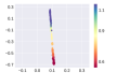
(a) Cheetah-dof

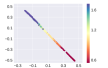
(b) Cheetah-torso

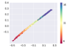
(c) Pendulum-gravity

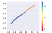
(d) Walker-gravity

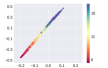
(e) Hopper-gravity

Figure 6: Representation visualization of DORA in all 6 MuJoCo tasks.

We present the representation visualization figures of all 6 MuJoCo tasks in Figure 6. With the color indicating the real parameters of dynamics, we find that the data points are sorted sequentially based on the real values of the varying parameters, which shows that the task representations capture the information of different task dynamics.

Moreover, we visualize the encodings of DORA in Cheetah-gravity with OOD dynamics, shown in Figure 7. It is evident to find that the representations in OOD dynamics (Figure 7(a)) are situated at both ends of the encodings in IID dynamics (Figure 7(b)). Such visualization results indicate that DORA learns generalizable representations, which can be extended to unseen OOD dynamics.

(a) In OOD dynamics

(b) In IID dynamics

Figure 7: Representation visulization in Cheetah-gravity. Left: In OOD dynamics. Right: In IID dynamics.

Appendix E Experiments in the Setting of OMRL

In the general OMRL setting, the algorithms are permitted to use a certain policy to collect context before evaluation. We compare the performance of DODA and other baselines in such a setting and the results are shown in figure 8. Benefiting from the effective task representations, DORA still exhibits a remarkable performance and outperforms the baselines in 5 of the total 6 MuJoCo tasks.

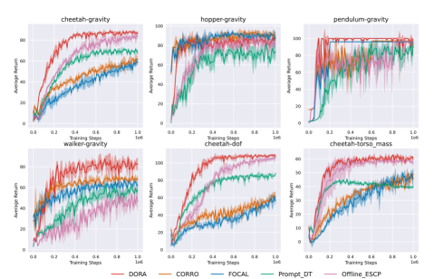
Figure 8: Test returns of DORA against the baselines in IID dynamics in the general OMRL setting. During meta-testing, a pre-collected context can be utilized to infer task representations before evaluation.

Appendix F Further Ablation Studies

F.1 Ablation Studies on the Losses

To visually illustrate the impact of the distortion loss and debias loss in DORA, we take the visualization results on Cheetah-gravity as an example. Figure 9(a) shows that the encoder can not extract informative representations without distortion loss. In addition, without the debias loss, representations inferred from tasks of similar dynamics no longer exhibit correlations as shown in Figure 9(b).

F.2 Ablation Studies on $\beta$

We conducted sensitivity tests on the hyper-parameter $\beta$ on 3 MuJoCo tasks, and the results indicate that excessively large or small values of $\beta$ lead to a decline in policy performance. Although in Pendulum-gravity, the case with $\beta=0.2$ shows better average performance, the policy performance sharply drops when $\beta=0$ (In Figure 5(a)). These experimental results, on the one hand, demonstrate that when $\beta$ is too small, the encoder struggles to debias representations from the behavior policy. On the other hand, when $\beta$ is too large, the diminishing effect of the distortion loss during the optimization process leads to a decrease in policy performance.

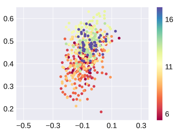
(a) Without Distortion Loss

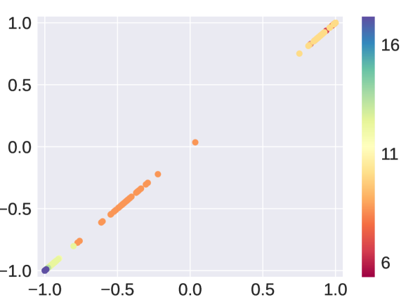
(b) Without Debias Loss

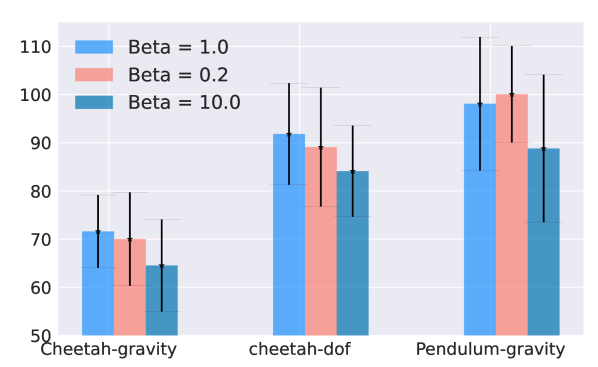
(c) Ablation Studies on $\beta$

Figure 9: Further ablation studies. Left: DORA without the distortion loss in Cheetah-gravity. Middle: DORA without debias loss in Cheetah-gravity. Right: Average normalized return of DORA with $\beta$ = 0.2, 1.0, and 10.0 over 5 random seeds. The error bar stands for the standard deviation.

References

- Chen et al. (2018) Chen, R. T., Li, X., Grosse, R. B., and Duvenaud, D. K. Isolating Sources of Disentanglement in Variational Autoencoders. In Advances in Neural Information Processing Systems, 2018.
- Cho et al. (2014) Cho, K., van Merrienboer, B., Gülçehre, Ç., Bahdanau, D., Bougares, F., Schwenk, H., and Bengio, Y. Learning Phrase Representations using RNN Encoder-Decoder for Statistical Machine Translation. In Conference on Empirical Methods in Natural Language Processing, 2014.
- Choi (2000) Choi, P.-M. Reinforcement learning in nonstationary environments. Hong Kong University of Science and Technology (Hong Kong), 2000.
- Finn et al. (2017) Finn, C., Abbeel, P., and Levine, S. Model-Agnostic Meta-Learning for Fast Adaptation of Deep Networks. In International Conference on Machine Learning, 2017.
- Fujimoto et al. (2019) Fujimoto, S., Meger, D., and Precup, D. Off-Policy Deep Reinforcement Learning without Exploration. In International Conference on Machine Learning, 2019.
- Gao et al. (2023) Gao, Y., Zhang, R., Guo, J., Wu, F., Yi, Q., Peng, S., Lan, S., Chen, R., Du, Z., Hu, X., et al. Context Shift Reduction for Offline Meta-Reinforcement Learning. arXiv preprint arXiv:2311.03695, 2023.
- Garcıa & Fernández (2015) Garcıa, J. and Fernández, F. A Comprehensive Survey on Safe Reinforcement Learning. Journal of Machine Learning Research, 16:1437–1480, 2015.
- Haarnoja et al. (2018) Haarnoja, T., Zhou, A., Abbeel, P., and Levine, S. Soft Actor-Critic: Off-Policy Maximum Entropy Deep Reinforcement Learning with a Stochastic Actor. In International Conference on Machine Learning, 2018.
- Kaiser et al. (2019) Kaiser, L., Babaeizadeh, M., Milos, P., Osinski, B., Campbell, R. H., Czechowski, K., Erhan, D., Finn, C., Kozakowski, P., Levine, S., et al. Model-Based Reinforcement Learning for Atari. arXiv preprint arXiv:1903.00374, 2019.
- Kaplanis et al. (2019) Kaplanis, C., Shanahan, M., and Clopath, C. Policy Consolidation for Continual Reinforcement Learning. In International Conference on Machine Learning, 2019.
- Khetarpal et al. (2022) Khetarpal, K., Riemer, M., Rish, I., and Precup, D. Towards Continual Reinforcement Learning: A Review and Perspectives. Journal of Artificial Intelligence Research, 75:1401–1476, 2022.
- Kidambi et al. (2020) Kidambi, R., Rajeswaran, A., Netrapalli, P., and Joachims, T. MOReL : Model-Based Offline Reinforcement Learning. In Advances in Neural Information Processing Systems, 2020.
- Kullback & Leibler (1951) Kullback, S. and Leibler, R. A. On information and sufficiency. The annals of mathematical statistics, 22(1):79–86, 1951.
- Kumar et al. (2020) Kumar, A., Zhou, A., Tucker, G., and Levine, S. Conservative Q-Learning for Offline Reinforcement Learning. In Advances in Neural Information Processing Systems, 2020.
- Levine et al. (2020a) Levine, S., Kumar, A., Tucker, G., and Fu, J. Offline Reinforcement Learning: Tutorial, Review, and Perspectives on Open Problems. arXiv preprint arXiv:2005.01643, 2020a.
- Levine et al. (2020b) Levine, S., Kumar, A., Tucker, G., and Fu, J. Offline reinforcement learning: Tutorial, review, and perspectives on open problems. arXiv preprint arXiv:2005.01643, 2020b.
- Li et al. (2021) Li, L., Yang, R., and Luo, D. FOCAL: Efficient Fully-Offline Meta-Reinforcement Learning via Distance Metric Learning and Behavior Regularization. In International Conference on Learning Representations, 2021.
- Lin et al. (2022a) Lin, R., Li, Y., Feng, X., Zhang, Z., Fung, X. H. W., Zhang, H., Wang, J., Du, Y., and Yang, Y. Contextual Transformer for Offline Meta Reinforcement Learning. arXiv preprint arXiv:2211.08016, 2022a.
- Lin et al. (2022b) Lin, S., Wan, J., Xu, T., Liang, Y., and Zhang, J. Model-Based Offline Meta-Reinforcement Learning with Regularization. In International Conference on Learning Representations, 2022b.
- Luo et al. (2022) Luo, F.-M., Jiang, S., Yu, Y., Zhang, Z., and Zhang, Y.-F. Adapt to Environment Sudden Changes by Learning a Context Sensitive Policy. In AAAI Conference on Artificial Intelligence, 2022.
- Mnih & Teh (2012) Mnih, A. and Teh, Y. W. A fast and simple algorithm for training neural probabilistic language models. In International Conference on Machine Learning, 2012.
- Nagabandi et al. (2019) Nagabandi, A., Clavera, I., Liu, S., Fearing, R. S., Abbeel, P., Levine, S., and Finn, C. Learning to Adapt in Dynamic, Real-World Environments through Meta-Reinforcement Learning. In International Conference on Learning Representations, 2019.
- Oord et al. (2018) Oord, A. v. d., Li, Y., and Vinyals, O. Representation Learning with Contrastive Predictive Coding. arXiv preprint arXiv:1807.03748, 2018.
- Rakelly et al. (2019) Rakelly, K., Zhou, A., Finn, C., Levine, S., and Quillen, D. Efficient Off-Policy Meta-Reinforcement Learning via Probabilistic Context Variables. In International Conference on Machine Learning, 2019.
- Ran et al. (2023) Ran, Y., Li, Y., Zhang, F., Zhang, Z., and Yu, Y. Policy Regularization with Dataset Constraint for offline reinforcement learning. In International Conference on Machine Learning, 2023.
- Ross & Bagnell (2010) Ross, S. and Bagnell, D. Efficient reductions for imitation learning. In International Conference on Artificial Intelligence and Statistics, 2010.
- Sohn et al. (2015) Sohn, K., Lee, H., and Yan, X. Learning Structured Output Representation using Deep Conditional Generative Models. In Advances in Neural Information Processing Systems, 2015.
- Sutton & Barto (2018) Sutton, R. and Barto, A. Reinforcement learning: An introduction. MIT press, 2018.
- Tishby & Zaslavsky (2015) Tishby, N. and Zaslavsky, N. Deep learning and the information bottleneck principle. In IEEE Information Theory Workshop, 2015.
- Tishby et al. (2000) Tishby, N., Pereira, F. C., and Bialek, W. The information bottleneck method. arXiv preprint arXiv: physics/0004057, 2000.
- Todorov et al. (2012) Todorov, E., Erez, T., and Tassa, Y. Mujoco: A Physics Engine for Model-Based Control. In International Conference on Intelligent Robots and Systems, pp. 5026–5033, 2012.
- Van der Maaten & Hinton (2008) Van der Maaten, L. and Hinton, G. Visualizing Data using t-SNE. Journal of machine learning research, 9(11), 2008.
- Wu et al. (2019) Wu, Y., Tucker, G., and Nachum, O. Behavior Regularized Offline Reinforcement Learning. arXiv preprint arXiv:1911.11361, 2019.
- Xu et al. (2022) Xu, M., Shen, Y., Zhang, S., Lu, Y., Zhao, D., Tenenbaum, J., and Gan, C. Prompting Decision Transformer for Few-Shot Policy Generalization. In International Conference on Machine Learning, 2022.
- Yu et al. (2020) Yu, T., Thomas, G., Yu, L., Ermon, S., Zou, J. Y., Levine, S., Finn, C., and Ma, T. MOPO: Model-based Offline Policy Optimization. In Advances in Neural Information Processing Systems, 2020.
- Yu et al. (2021) Yu, T., Kumar, A., Rafailov, R., Rajeswaran, A., Levine, S., and Finn, C. COMBO: Conservative Offline Model-Based Policy Optimization. In Advances in Neural Information Processing Systems, 2021.
- Yuan & Lu (2022) Yuan, H. and Lu, Z. Robust Task Representations for Offline Meta-Reinforcement Learning via Contrastive Learning. In International Conference on Machine Learning, 2022.
- Zhou et al. (2023) Zhou, R., Gao, C.-X., Zhang, Z., and Yu, Y. Generalizable Task Representation Learning for Offline Meta-Reinforcement Learning with Data Limitations. arXiv preprint arXiv:2312.15909, 2023.