Contraction of Markovian Operators in Orlicz Spaces
and Error Bounds for Markov Chain Monte Carlo

Abstract

We introduce a novel concept of convergence for Markovian processes within Orlicz spaces, extending beyond the conventional approach associated with $L_{p}$ spaces. After showing that Markovian operators are contractive in Orlicz spaces, our key technical contribution is an upper bound on their contraction coefficient, which admits a closed-form expression. The bound is tight in some settings, and it recovers well-known results, such as the connection between contraction and ergodicity, ultra-mixing and Doeblin’s minorisation. Specialising our approach to $L_{p}$ spaces leads to a significant improvement upon classical Riesz-Thorin’s interpolation methods. Furthermore, by exploiting the flexibility offered by Orlicz spaces, we can tackle settings where the stationary distribution is heavy-tailed, a severely under-studied setup. As an application of the framework put forward in the paper, we introduce tighter bounds on the mixing time of Markovian processes, better exponential concentration bounds for MCMC methods, and better lower bounds on the burn-in period. To conclude, we show how our results can be used to prove the concentration of measure phenomenon for a sequence of Markovian random variables.

I Introduction

The topic of bounding the contraction coefficient of Markovian operators in $L_{p}$ spaces and, specifically, $L_{2}$ spaces has a rich history, see the survey by [1]. The motivation comes from the fact that, whenever the contraction coefficient is strictly smaller than $1$, the corresponding Markovian process converges exponentially fast to the stationary distribution [2]. Moreover, the characterisation of the contraction coefficient also yields upper bounds on the so-called “mixing times” of the process, i.e., the number of steps required to be close to the stationary distribution. This has practical implications in Markov Chain Monte Carlo (MCMC) methods: MCMC allows estimating integrals with respect to a certain measure $\pi$ when said measure is either inaccessible or cannot be sampled efficiently, by designing a Markov chain that approximates it [3, 4, 2]. A big effort has thus been devoted to understanding how the estimation error behaves and how long the Markov chain needs to get close enough to the limiting distribution (burn-in period) [3, 4, 2].

Most of the literature focuses on asymptotic analyses [3] or mean-squared error bounds [2, 5], and it is restricted to finite-state space Markov chains. A different line of work tackles the problem by providing concentration inequalities for dependent random variables [6, 7, 8, 9, 10, 11, 12], which lead to high-probability error bounds and characterisations of the burn-in period. We highlight that all these results rely on the contraction coefficient of the Markov kernel associated with the chain. Similarly, but through a different route, [13] proves that one can control the mixing times of a Markov chain by studying the strong data-processing inequality (SDPI) constant of various divergences.

Our work delivers new and improved bounds on these fundamental quantities, by stepping away from the more classical framework and considering Orlicz spaces, a generalisation of $L_{p}$ spaces. We show that, as for $L_{p}$, Markov kernels are contractive in Orlicz spaces, i.e., the contraction coefficients of Markov kernels are less than or equal to $1$. We can then define a notion of convergence of Markov processes, which depends on the corresponding contraction coefficient. In particular, our main result, Theorem 3, provides an upper bound for the contraction coefficient of Markovian operators, which admits a closed-form expression. The key technical novelties come from duality considerations: the convergence of a Markovian process determined by $K$ depends on the contraction coefficient of its dual $K^{\star}$, which can in turn be bounded by considering appropriate nested norms of densities of $K^{\star}$ with respect to the stationary measure.

Our approach stands out as the first of its kind, as it does not rely on the existence of a spectral gap. In contrast, most existing bounds are based on the spectral gap [2, 11] and, thus, hold in $L_{2}$. To handle $L_{p}$ spaces, the typical strategy is then to leverage Riesz-Thorin’s interpolation, which often leads to vacuous bounds. In contrast, Theorem 3 evades said restrictions by considering directly the contraction coefficient in $L_{p}$, thus vastly improving upon the state of the art. Leveraging arbitrary Orlicz spaces allows us to also consider distributions with heavy tails, which are hard to handle with classical techniques [14, 15], see Remark 3.

Theorem 3 recovers well-known theorems in the literature, i.e., the connection between contraction and ergodicity (Corollary 1), as well as ultra-mixing and Doeblin’s minorisation (Corollary 2) [16, 17, 13]. As an application of our analysis, we give better bounds on the mixing times of Markovian processes (Section IV-A) and better convergence guarantees for MCMC methods (Section IV-B), which lead to more refined bounds on the burn-in period [2, 11]. Finally, by exploiting the strategy developed by [12], we provide improved concentration results for a sequence of dependent random variables, where the dependence is captured by a Markovian process.

II Preliminaries

We adopt a measure-theoretic framework. Given a measurable space $(\mathcal{X},\mathcal{F})$ and two measures $\mu,\nu$ making it a measure space, if $\nu$ is absolutely continuous w.r.t. $\mu$ ($\nu\ll\mu$), we represent with $\frac{d\nu}{d\mu}$ the Radon-Nikodym derivative of $\nu$ w.r.t. $\mu$. Given a (measurable) function $f:\mathcal{X}\to\mathbb{R}$ and a measure $\mu$, we denote with $\mu(E)$ the measure of an event $E$ and with $\mu(f)=\int fd\mu$ the Lebesgue integral of $f$ with respect to the measure $\mu$ .

II-A Markov kernels and Markov chains

Definition 1 (Markov kernel).

Let $(\Omega,\mathcal{F})$ be a measurable space. A Markov kernel $K:\mathcal{F}\times\Omega\to[0,1]$ is such that (i) $\forall\,x\in\Omega$, the mapping $E\in\mathcal{F}\to K(E|x)$ is a probability measure on $(\Omega,\mathcal{F})$, and (ii) $\forall\,E\in\mathcal{F}$, the mapping $x\in\Omega\to K(E|x)$ is an $\mathcal{F}$-measurable real-valued function.

A Markov kernel acts on measures “from the right”, i.e., given a measure $\mu$ on $(\Omega,\mathcal{F})$, $\mu K(E)=\mu(K(E|\cdot))=\int d\mu(x)K(E|x),$ and on functions “from the left”, i.e., given a function $f:\Omega\to\mathbb{R}$, $Kf(x)=\int dK(y|x)f(y).$ Hence, given a function $f\in L^{p}(\mu)$, one can see $K$ as a mapping $K:L^{p}(\mu)\to L^{p}(\mu)$. Moreover, an application of Jensen’s inequality gives that $\mu((Kf)^{p})\leq\mu(K(f^{p}))=\mu K(f^{p})$, thus the mapping can be extended to $K:L^{p}(\mu)\to L^{p}(\mu K)$.

Given a Markov kernel $K$ and a measure $\mu$, let $K^{\star}_{\mu}$ denote the dual operator. By definition, the dual kernel can be seen as acting on $(L^{p}(\mu K))^{\star}\cong L^{q}(\mu K)$ with $q=\frac{p-1}{p}$ and returning a function in $(L^{p}(\mu))^{\star}\cong L^{q}(\mu)$. In particular, given a probability measure $\mu$ and two measurable functions $f,g$, one can define the inner-product $\langle f,g\rangle_{\mu}=\int(f\cdot g)d\mu,$ and $K^{\star}_{\mu}$ is the operator such that $\langle Kf,g\rangle_{\mu}=\langle f,K^{\star}_{\mu}g\rangle_{\mu K}$, for all $f$ and $g$. In discrete settings, the dual operator can be explicitly characterised via $K$ and $\mu$ as $K_{\mu}^{\star}(y|x)=K(y|x)\mu(x)/\mu K(y)$, see [13, Eq. (1.2)].

Given a sequence of random variables $(X_{t})_{t\in\mathbb{N}}$, one says that it represents a Markov chain if, given $i\geq 1$, there exists a Markov kernel $K_{i}$ such that for every measurable event $E$:

$$\mathbb{P}(X_{i}\in E|X_{1},\ldots,X_{i-1})=\mathbb{P}(X_{i}\in E|X_{i-1})=K_{i}(E|X_{i-1})\qquad\text{ almost surely}.$$ (1)

If for every $i\geq 1$, $K_{i}=K$ for some Markov kernel $K$, then the Markov chain is time-homogeneous, and we suppress the index from $K$. The kernel $K$ of a Markov chain is the probability of getting from $x$ to $E$ in one step, i.e., for every $i\geq 1$, $K(E|x)=\mathbb{P}(X_{i}\in E|X_{i-1}=x)$. One can then define (inductively) the $t$-step kernel $K^{t}$ as $K^{t}(E|x)=\int K^{t-1}(E|y)dK(y|x)$. Note that $K^{t}$ is also a Markov kernel, and it represents the probability of getting from $x$ to $E$ in $\kappa$ steps: $K^{t}(E|x)=\mathbb{P}(X_{t+1}\in E|X_{1}=x)$. If $(X_{t})_{t\in\mathbb{N}}$ is the Markov chain associated to the kernel $K$ and $X_{0}\sim\mu$, then $\mu K^{m}$ denotes the measure of $X_{m+1}$ at every $m\in\mathbb{N}$. Furthermore, a probability measure $\pi$ is a stationary measure for $K$ if $\pi K(E)=\pi(E)$ for every measurable event $E$. When the state space is discrete, $K$ can be represented via a stochastic matrix.

Given a Markov kernel and a measure, one can define the corresponding dual [16] and show the following result, which is pivotal for characterising the convergence of a Markovian process to the stationary measure. The proof is deferred to Appendix A-B.

Lemma 1.

Let $\mu$ be a positive measure, $\nu$ a positive measure s.t. $\nu\ll\mu$, and $f$ the Radon-Nikodym derivative $\frac{d\nu}{d\mu}$. Let $K$ be a Markov kernel and $g=\frac{d\nu K}{d\mu K}$. Then,

$$g=K_{\mu}^{\star}f\hskip 20.00003pt\mu\text{-a.e.},$$ (2)

where $K_{\mu}^{\star}$ is the operator such that, given two functions $f,g$, one has that $\langle Kh,f\rangle_{\mu}=\langle h,K_{\mu}^{\star}f\rangle.$

Furthermore, $K^{\star}_{\mu}$ can be proved to Markovian [16, Section 2, Lemma 2.2].

II-B Orlicz spaces

Definition 2 (Young Function, [18, Chapter 3]).

Let $\psi:\mathbb{R}^{+}\to\mathbb{R}^{+}$ be a convex non-decreasing function s.t. $\psi(0)=0$ and $\psi(x)\xrightarrow[x\to\infty]{}\infty$. Then, $\psi$ is called a Young function.

Definition 3 ([18, Definition 5]).

Let $\psi$ be a Young function. Let $(\Omega,\mathcal{F},\mu)$ be a measure space and denote with $L_{0}(\mu)$ the space of all the $\mathcal{F}$-measurable and real-valued functions on $\Omega$. An Orlicz space can be defined as the following set:

$$L_{\psi}(\mu)=\left\{f\in L_{0}(\mu):\int_{\Omega}\psi(|\lambda f|)d\mu<+\infty\text{ for some }\lambda>0\right\}.$$ (3)

Given a Young function $\psi:[0,+\infty)\to\overline{\mathbb{R}}^{+}$, the complementary function to $\psi$ in the sense of Young, denoted as $\psi^{\star}:\mathbb{R}\to\overline{\mathbb{R}}^{+}$, is defined as follows [18, Section 1.3]:

$$\psi^{\star}(x)=\sup\left\{\lambda|x|-\psi(\lambda):\lambda\geq 0\right\}.$$ (4)

An Orlicz space can be endowed with several norms that render it a Banach space [19]: the Luxemburg norm, the Orlicz norm, and the Amemiya norm. We will henceforth ignore the Orlicz norm, as it is equivalent to the Amemiya norm [19], and we define the Luxemburg norm $L_{\psi}^{L}$ and the Amemiya norm $L_{\psi}^{A}$ as

$$\lVert f\rVert_{L^{L}_{\psi}(\mu)}=\inf\left\{\sigma>0:\mu\left(\psi\left(|f|/\sigma\right)\right)\leq 1\right\},\qquad\lVert f\rVert_{L^{A}_{\psi}(\mu)}=\inf_{t>0}\frac{\mu\left(\psi(t|f|)\right)+1}{t}.$$ (5)

Orlicz spaces and the corresponding norms recover well-known objects (e.g., $L_{p}$-norms) and characterise random variables according to their “tail”. For more details, see Appendix A-A.

III Contraction of Markov kernels

The contractivity of Markov operators has been studied in particular for $L^{p}$ spaces, with [16, 20] considering Orlicz spaces as well. As we prove results for both Amemiya and Luxemburg norms, we use $\left\lVert\cdot\right\rVert_{L_{\psi}^{N}(\mu)}$ with $N\in\{A,L\}$ to denote both norms and we use $\left\lVert\cdot\right\rVert_{L_{\psi}^{N^{\star}}(\mu)}$ for the corresponding dual norm (e.g., if $N=A$ and one has an Amemiya norm, then $N^{\star}=L$ and the dual is the Luxemburg norm).

Definition 4.

Let $\psi$ be a Young functional, $N\in\{A,L\}$ and $K$ a Markov kernel. The contraction coefficients of $K$ in the spaces $L_{\psi}(\mu),L_{\psi}^{0}(\mu)$ are denoted as follows:

$$\sup_{f\in L_{\psi}(\mu)}\frac{\left\lVert Kf\right\rVert_{L_{\psi}^{N}(\mu)}}{\left\lVert f\right\rVert_{L_{\psi}^{N}(\mu)}}=\left\lVert K\right\rVert_{L_{\psi}^{N}(\mu)\to L_{\psi}^{N}(\mu)},\qquad\sup_{f\in L_{\psi}^{0}(\mu)}\frac{\left\lVert Kf\right\rVert_{L_{\psi}^{N}(\mu)}}{\left\lVert f\right\rVert_{L_{\psi}^{N}(\mu)}}=\left\lVert K\right\rVert_{L_{\psi}^{N,0}(\mu)\to L_{\psi}^{N,0}(\mu)},$$ (6)

where $L_{\psi}^{0}(\mu)$ denotes the closed subspace of functions with mean $0$, i.e., $L_{\psi}^{0}(\mu)=\{f\in L_{\psi}(\mu):\mu(f)=0\}$. Whenever the measure is clear from the context, for ease of notation, we denote the contraction coefficient as $\left\lVert K\right\rVert_{L_{\psi}^{N}\to L_{\psi}^{N}}$.

A characterisation of how Markovian operators behave in Orlicz spaces is stated below and proved in Appendix C-A.

Theorem 1.

Let $\psi$ be a Young functional, $N\in\{A,L\}$, and $K$ a Markov kernel with stationary distribution $\pi$. Then, for every $f\in L_{\psi}(\pi)$,

$$\left\lVert Kf\right\rVert_{L^{N}_{\psi}(\pi)}\leq\left\lVert f\right\rVert_{L^{N}_{\psi}(\pi)}\hskip 20.00003pt \text{and}\hskip 20.00003pt\left\lVert K\right\rVert_{L^{N}_{\psi}\to L^{N}_{\psi}}=1.$$ (7)

The key takeaway of Theorem 1 is that, as in $L_{p}$ spaces, Markov kernels are contractive, but on the general space of $L_{\psi}$-integrable functions said contraction coefficient is trivially $1$. Restricting to the closed subspace of functions with mean $0$ (i.e., $L^{0}_{\psi}(\mu)$) does yield an improvement. In fact, the contraction coefficient of a Markov kernel $K$ in $L_{\psi}^{0}$ is typically less than $1$. This observation is fundamental to characterise convergence to the stationary distribution. Indeed, if $\left\lVert K\right\rVert_{L_{2}^{0}\to L_{2}^{0}}=\gamma<1$, then $K$ admits an $L_{2}$-spectral gap $(1-\gamma)$, which implies “$L_{2}$-geometric ergodicity”, as stated below [2, Proposition 3.12].

Proposition 1.

Let $K$ be a Markov kernel with stationary distribution $\pi$ and spectral gap $1-\gamma>0$. For every probability measure $\nu$ on the same space s.t. $\left\lVert d\nu/d\pi\right\rVert_{L_{2}(\pi)}<\infty$, we have

$$\left\lVert\nu K^{t}-\pi\right\rVert_{L_{2}(\pi)}\leq\gamma^{t}\left\lVert\nu-\pi\right\rVert_{L_{2}(\pi)}.$$ (8)

In fact, in the specific setting of $L_{2}$, geometric ergodicity and existence of a spectral gap are equivalent notions [2, Proposition 3.13].

The purpose of this work is to relate the contractivity of Markovian operators on Orlicz spaces to the convergence of the corresponding Markov chain to its stationary distribution. To do so, we leverage Lemma 1 and show convergence in $L_{\psi}^{N}$-norm, as soon as the contraction coefficient of the dual kernel ${K}^{\star}$ is $<1$. This is formalised in the result below, which is proved in Appendix C-B.

Theorem 2.

Let $K$ be a Markov kernel with stationary distribution $\pi$, $N\in\{A,L\}$, and $\psi$ a Young functional. For every measure $\nu\ll\pi$ and $t\in\mathbb{N}$, we have

$$\left\lVert\frac{d\nu K^{t}}{d\pi}-1\right\rVert_{L^{N}_{\psi}(\pi)}\leq\left\lVert{K}^{\star}\right\rVert_{L_{\psi}^{N,0}\to L_{\psi}^{N,0}}^{t}\left\lVert\frac{d\nu}{d\pi}-1\right\rVert_{L_{\psi}^{N}(\pi)}.$$ (9)

Theorem 2 links the convergence of a Markovian process to the contraction coefficient of the dual kernel $K^{\star}$. Indeed, if $\left\lVert{K}^{\star}\right\rVert_{L_{\psi}^{N,0}}<1$, then the right-hand side of Equation 9 goes to $0$ exponentially fast in the number of steps $t$ and, hence, $\nu K^{\infty}=\pi$. We also note that the proof can be adapted to replace $\left\lVert{K}^{\star}\right\rVert_{L_{\psi}^{N,0}\to L_{\psi}^{N,0}}^{t}$ with $\left\lVert{K}^{\star}-1_{\pi}\right\rVert^{t}_{L_{\psi}^{N}\to L_{\psi}^{N}}$, where $1_{\pi}$ is the operator mapping a function $f$ to $\int fd\pi$. These two bounds are closely related: $\left\lVert{K}^{\star}\right\rVert_{L_{\psi}^{N,0}\to L_{\psi}^{N,0}}^{t}$ focuses on $0$-mean functions, while in $\left\lVert{K}^{\star}-1_{\pi}\right\rVert^{t}_{L_{\psi}^{N}\to L_{\psi}^{N}}$ we directly subtract the mean $1_{\pi}$. More generally, we can relate the contraction coefficient of $K^{\star}$ on $L_{\psi}^{0}$ to that of $K^{\star}-1_{\pi}$ on $L_{\psi}$, see Section A-C.

At this point, we are ready to state our key technical contribution which bounds the contraction coefficient of a kernel and of its dual. Its proof is in Section C-C.

Theorem 3.

Let $\psi$ be a Young functional and $\mu$ a probability measure. Let $K$ be a Markov kernel, $K^{\star}=K^{\star}_{\mu}$ its dual, and $N\in\{A,L\}$. Assume that, for every $x$, $K(\cdot|x)$ is absolutely continuous w.r.t. $\mu K$ and, for every $y$, $K^{\star}(\cdot|y)$ is absolutely continuous w.r.t. $\mu$. Denote with $g_{x}=\frac{dK(\cdot|x)}{d\mu K}$ and $g_{y}=\frac{dK^{\star}(\cdot|y)}{d\mu}$ the Radon-Nikodym derivatives. Then, for every $f\in L_{\psi}^{0}(\mu K)$ and $h\in L_{\psi}^{0}(\mu)$,

$$\frac{\left\lVert Kf\right\rVert_{L_{\psi}^{N}(\mu)}}{\left\lVert f\right\rVert_{L_{\psi}^{N}(\mu K)}}\leq\left\lVert\left\lVert g_{X}-1\right\rVert_{L_{\psi^{\star}}^{N^{\star}}(\mu K)}\right\rVert_{L_{\psi}^{N}(\mu)}\text{ and }\hskip 10.00002pt\frac{\left\lVert K^{\star}h\right\rVert_{L_{\psi}^{N}(\mu K)}}{\left\lVert h\right\rVert_{L_{\psi}^{N}(\mu)}}\leq\left\lVert\left\lVert g_{Y}-1\right\rVert_{L_{\psi^{\star}}^{N^{\star}}(\mu)}\right\rVert_{L_{\psi}^{N}(\mu K)}.$$ (10)

Remark 1.

Let $\psi(x)=|x|^{p}$ for $p>1$, and $q=p/(p-1)$. Then, the following is a corollary of Theorem 3 that holds for every $f\in L_{p}^{0}(\mu K)$ and $h\in L_{\psi}^{0}(\mu)$:

$$\frac{\left\lVert Kf\right\rVert_{L_{p}(\mu)}}{\left\lVert f\right\rVert_{L_{p}(\mu K)}}\leq\left\lVert\left\lVert g_{X}-1\right\rVert_{L_{q}(\mu K)}\right\rVert_{L_{p}(\mu)}\text{ and }\hskip 10.00002pt\frac{\left\lVert K^{\star}h\right\rVert_{L_{p}(\mu K)}}{\left\lVert h\right\rVert_{L_{p}(\mu)}}\leq\left\lVert\left\lVert g_{Y}-1\right\rVert_{L_{q}(\mu)}\right\rVert_{L_{p}(\mu K)}.$$ (11)

Theorem 3 offers a closed-form bound on the contraction coefficient. We remark that, to the best of our knowledge, no such bound in $L_{\psi}^{0}$ spaces exists. If the kernel is induced by the so-called binary symmetric channel of parameter $\lambda$ ($K(x|y)=1-\lambda$ for $x=y$; otherwise, $K(x|y)=\lambda$), then Equation 11 is tight for $p=2$, see Example 2 in Appendix B for details. The case of $p=\infty$ represents another setting in which we can prove the tightness of Equation 11, as formalised below and proved in Section C-D.

Corollary 1.

Let $K$ be a Markov kernel with stationary distribution $\pi$. Then, the following holds:

$$\left\lVert K^{t}-1_{\pi}\right\rVert_{L_{\infty}\to L_{\infty}}\leq\left\lVert\left\lVert g^{t}_{X}-1\right\rVert_{L_{1}(\pi)}\right\rVert_{L_{\infty}(\pi)}=\operatorname*{ess\,sup}_{\pi}2\left\lVert K^{t}(\cdot|X)-\pi\right\rVert_{TV},~{}$$ (12)

where $g_{x}^{t}(y)=\frac{dK^{t}(y|x)}{d\pi K^{t}(y)}=\frac{dK^{t}(y|x)}{d\pi(y)}$.

In fact, $\left\lVert K^{t}-1_{\pi}\right\rVert_{L_{\infty}\to L_{\infty}}=\operatorname*{ess\,sup}_{x}2\left\lVert K^{t}(\cdot|x)-\pi\right\rVert_{TV}$ by Proposition 3.23 in [2]. In the Markov chain literature, it is quite common to show that the right-hand side of Equation 12 is bounded. This usually goes under the name of uniform (or strong) ergodicity. Hence, Corollary 1 leads to another proof that asking for uniform ergodicity implies $L_{\infty}$-exponential convergence.

Theorem 3 also recovers other well-known results. Indeed, [16] show that, if ultra-mixing holds (which, in turn, implies Doebling’s minorisation [17, Section 4.3.3]), then one can bound the contraction coefficient of Markovian kernels in arbitrary norms.

Corollary 2.

Given a Markov kernel $K$, assume there exists $0<\epsilon<1$ s.t. the kernel satisfies the ultra-mixing condition, i.e., for all $x,y$,

$$\frac{dK(\cdot|x)}{dK(\cdot|y)}\geq\epsilon,\hskip 20.00003ptK(\cdot|y)-a.e.$$ (13)

Then, for every Young function $\psi$ and $N\in\{A,L\}$, we have

$$\left\lVert\frac{d\nu K}{d\mu K}-1\right\rVert_{L^{N}_{\psi}(\mu K)}\leq(1-\epsilon)\left\lVert\frac{d\nu}{d\mu}-1\right\rVert_{L^{N}_{\psi}(\mu)}.$$ (14)

Corollary 2 is indeed a consequence of Theorem 3, as proved in Section C-E.

IV Applications

IV-A Mixing times

Definition 5.

Given a Markov kernel $K$ with stationary distribution $\pi$, $N\in\{A,L\}$, and a Young functional $\psi$, the $\psi$-mixing time of $K$ is the function $\tau_{\psi}(K,\cdot):\mathbb{R}^{+}\to\mathbb{N}$ such that

$$\tau_{\psi}(K,\epsilon)=\min\left\{t\in\mathbb{N}:\sup_{\nu}\left\lVert\frac{d\nu K^{t}}{d\pi}-1\right\rVert_{L_{\psi}^{N}(\pi)}\leq\epsilon\right\}.$$ (15)

The first application of our framework is stated below and follows from Theorem 3 and Eq. (15).

Corollary 3.

Let $K$ be a Markov operator with stationary distribution $\pi$, $K^{\star}=K^{\star}_{\pi}$ its dual, $N\in\{A,L\}$, and $\psi$ a Young functional. Then, the following holds:

$$\tau_{\psi}(K,\epsilon)\leq\frac{\log\left(\left(\sup_{\nu}\left\lVert\frac{d\nu}{d\pi}-1\right\rVert_{L_{\psi}^{N}(\pi)}\right)/\epsilon\right)}{-\log\left(\left\lVert K^{\star}\right\rVert_{L_{\psi}^{N,0}\to L_{\psi}^{N,0}}\right)}.$$ (16)

Remark 2.

For discrete spaces and a discrete-valued Markov kernel, by leveraging the convexity of the norms and the fact that convex functions on a compact convex set attain their maximum on an extreme point, we can upper bound $\left\lVert\frac{d\nu}{d\pi}-1\right\rVert_{L_{\psi}^{N}(\pi)}$ with $\max_{x}\left\lVert\frac{d\delta_{x}}{d\pi}-1\right\rVert_{L_{\psi}^{N}(\pi)}$, which admits a closed-form expression. See Section D-A for details.

Corollary 3 relates the contraction coefficient of the dual operator to the mixing time of the corresponding Markov chain, thus motivating our study of said contraction coefficient. Moreover, as $\psi$ is arbitrary, a natural question concerns the choice of the norm. To address it, first we derive a general result providing intuition over what it means to be close in a specific norm. In particular, we relate the probability of any event under $\mu K^{t}$ with the probability of the same event under the stationary measure $\pi$ and an $L^{N}_{\psi}$-norm. We then focus on the well-known family of $L_{p}$-norms (particularly relevant for exponentially decaying probabilities under $\pi$), and show that asking for a bounded norm with larger $p$ guarantees a faster decay of the probability of the same event under $\mu K^{t}$. Finally, we design a Young function tailored to the challenging (and less understood) setting in which $\pi$ behaves like a power law [14].

Theorem 4.

Let $t\in\mathbb{N}$ and $E$ be a measurable event. Then,

$$\mu K^{t}(E)\leq\min\begin{cases}\inf_{\psi}1/{\psi^{\star}}^{-1}(1/\pi(E))\left(\left\lVert\frac{d\mu K^{t}}{d\pi}-1\right\rVert_{L_{\psi}^{A}(\pi)}+{\psi^{\star}}^{-1}(1)\right),\\ \inf_{\psi}\pi(E)\psi^{-1}(1/\pi(E))\left(\left\lVert\frac{d\mu K^{t}}{d\pi}-1\right\rVert_{L_{\psi}^{L}(\pi)}+1/\psi^{-1}(1)\right),\end{cases}$$ (17)

where the infimum is over all Young functionals $\psi$.

We now apply Theorem 4 to various $\psi$, and start by demonstrating the advantage of considering $L_{p}$-norms with $p\neq 2$. The result below is proved in Section D-C.

Corollary 4.

Let $\varphi_{p}(x)=|x|^{p}/p$ with $p>1$, $q=p/(p-1)$, $t\in\mathbb{N}$ and $E$ a measurable event. Then,

$$\mu K^{t}(E) \leq\pi(E)^{\frac{1}{q}}\left(\pi(E)^{\frac{1}{p}}+\left\lVert\frac{d\mu K^{t}}{d\pi}-1\right\rVert_{L_{p}(\pi)}\right).$$ (18)

As an immediate consequence, if $\left\lVert\frac{d\mu K^{t}}{d\pi}-1\right\rVert_{L_{p}(\pi)}\leq\epsilon,$ then for every $E$

$$\mu K^{t}(E) \leq\pi(E)^{\frac{1}{q}}\left(\pi(E)^{\frac{1}{p}}+\epsilon\right)=\pi(E)+\pi(E)^{\frac{1}{q}}\epsilon.$$ (19)

The following setting is especially interesting for the applicability of Corollary 4. Consider a function $f:\mathcal{X}^{n}\to\mathbb{R}$ and $E=\{(x_{1},\ldots,x_{n}):|f(x_{1},\ldots,x_{n})-\pi(f)|\geq\eta\}$ for some fixed $\eta>0$. If $f(x_{1},\ldots,x_{n})=\frac{1}{n}\sum_{i=1}^{n}f_{i}(x_{i})$ for $f_{1},\ldots,f_{n}$ with $0\leq f_{i}(x)\leq C$, by Hoeffding’s inequality one has:

$$\pi(E)\leq 2\exp\left(-\frac{2\eta^{2}n}{C^{2}}\right),$$ (20)

where the constant $C^{2}$ at the exponent can be improved under additional assumptions, see e.g. [21]. Then, given $t\geq\tau_{\varphi_{p}}(K,\epsilon)$ and $q=\frac{p}{p-1}$, we have

$$\mu K^{t}(E)\leq 2\exp\left(-\frac{2n\eta^{2}}{C^{2}}\right)+\epsilon 2^{\frac{1}{q}}\exp\left(-\frac{2n\eta^{2}}{qC^{2}}\right).$$ (21)

Starting from Equation 21, one can now select $\epsilon$ such that the probability is exponentially decaying in the dimension of the ambient space $n$. In fact, a bound that decays exponentially in the dimension $n$ is guaranteed whenever, for a given $\eta$, $f$, and finite $p$,

$$\epsilon<\exp\left(\gamma\frac{2n\eta^{2}}{qC^{2}}\right),\text{ with }\gamma<1.$$ (22)

For example, $\epsilon=\exp\left(n\eta^{2}/qC^{2}\right)$ guarantees exponential convergence in Equation 21 and plugging this choice in Equation 16 gives the bound below on the mixing time:

$$\tau_{p}(K,\epsilon)\leq\frac{1}{-\log\left(\left\lVert K^{\star}\right\rVert_{L_{p}^{0}\to L_{p}^{0}}\right)}\left(\log\left(L_{p}^{\star}(\pi)\right)+\frac{qC^{2}}{n\eta^{2}}\right),$$ (23)

where $L_{p}^{\star}(\pi)=\sup_{\nu\ll\pi}\left\lVert\frac{d\nu}{d\pi}-1\right\rVert_{L^{p}(\pi)}$. We note that, besides $\epsilon$, both $L_{p}^{\star}(\pi)$ and $\left\lVert K^{\star}\right\rVert_{L_{p}^{0}\to L_{p}^{0}}$ depend on the dimension $n$. To maximise the rate of exponential decay in Equation 21, one has to take $p\to\infty$, which implies $q\to 1$. The price to pay is an increase of the mixing time and, to quantify such increase, it is crucial to provide tight bounds on the contraction coefficient of Markovian operators, beyond the usual $L_{2}$ space. Theorem 3 can then be leveraged to compute said bounds, and we now compare it with the standard approach in the literature, i.e., the Riesz-Thorin interpolation theorem between norms, which is stated below for convenience.

Proposition 2.

Let $p\in(1,+\infty)$ and $t\in\mathbb{N}$. Let $K$ be a Markov kernel with stationary distribution $\pi$. If $K$ admits an $L_{2}$-spectral gap of $(1-\gamma)$, then the following holds:

$$\left\lVert K^{t}-1_{\pi}\right\rVert_{L_{p}\to L_{p}}\leq\begin{cases}2^{1/p}\gamma^{2t\frac{p-1}{p}},&p\in(1,2),\\ 2^{2\frac{p-1}{p}}\gamma^{2t/p},&p\in(2,+\infty).\end{cases}$$ (24)

Moreover, one has that:

$$\left\lVert K^{t}-1_{\pi}\right\rVert_{L_{2}\to L_{2}}\leq\gamma^{t}\text{ , }\quad\left\lVert K^{t}-1_{\pi}\right\rVert_{L_{1}\to L_{1}}\leq 2\text{ , }\quad\left\lVert K^{t}-1_{\pi}\right\rVert_{L_{\infty}\to L_{\infty}}\leq 2.$$ (25)

As an example, consider the binary symmetric channel of parameter $\lambda$. Then, $\gamma=(1-2\lambda)$ and Proposition 2 with $p>2$ yields:

$$\left\lVert K^{t}-1_{\pi}\right\rVert_{L_{p}\to L_{p}}\leq 2^{2\frac{p-1}{p}}(1-2\lambda)^{2t/p}.$$ (26)

In contrast, Theorem 3 gives:

$$\left\lVert K^{t}-1_{\pi}\right\rVert_{L_{p}\to L_{p}}\leq(1-2\lambda)^{t},\text{ for every }p\geq 1,$$ (27)

which improves over Equation 26 for every $p$. Notably, Equation 27 holds even if $p\to 1$ and $p\to\infty$, while the result of Proposition 2 is vacuous in both cases (cf. Equation 25). Furthermore, Figure 2 considers Markov kernels induced by $5\times 5$ randomly generated stochastic matrices, and it shows that while the bound in Proposition 2 is always vacuous (red dots), the bound given by Equation 11 is always below $1$ and often very close to $0$ (blue dots).

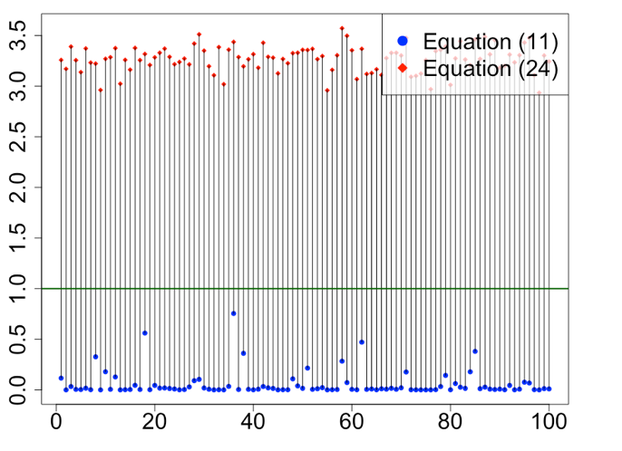
Figure 1: Bound on the contraction coefficient given by Equations 11 and 24 in $100$ randomly generated $5\times 5$ stochastic matrices, for $p=100$ and $t=10$.

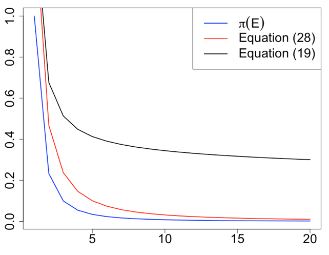
Figure 2: Bound on $\mu K^{t}(E)$, as a function of $n$, induced by the $L_{1.09}$-norm (Eq. (19)) and $L_{\psi_{5}^{5}}^{L}$ (Eq. 28), when $\pi(E)$ decays polynomially with exponent $-2.1$.

Remark 3.

A suitable choice of the Young function allows to treat stationary distributions with heavy tails. In this case, geometric or uniform ergodicity cannot be achieved, and the best one can hope for is a polynomial convergence in Total Variation [14]. Thus, there is no spectral gap [22, Theorem 2.1], which affects the convergence rates of MCMC algorithms with polynomial target distributions, e.g., Metropolis-Hastings with independence sampler [15, Section 4.3].

For concreteness, consider upper bounding $\mu K^{t}(E)$, when the stationary distribution $\pi$ is a power-law with exponent $-(2+\eta)$ and $t$ is s.t. $\left\lVert\frac{d\mu K^{t}}{d\pi}-1\right\rVert_{L_{p}(\pi)}\leq\epsilon$. Then, if we restrict to $L_{p}$ spaces, we obtain the bound in Equation 19, with $q>(1+\eta)/\eta$. Here, the lower bound on $q$ comes from the fact that $q=\frac{p}{p-1}$ and the largest $p$ s.t. a random variable with measure $\pi$ belongs to $L_{p}$ has to satisfy $1<p<1+\eta$ ($p=1$ implies $q=\infty$ leading to a trivial bound in  Equation 19).

Instead, by considering Orlicz spaces different from $L_{p}$, much more refined bounds can be obtained. Let $\psi_{k}^{m}(x)=x^{m}\mathbbm{1}_{1\leq x\leq k}+((1+x)\log(1+x)+k^{m}-(1+k)\log(1+k))\mathbbm{1}_{x>k}$, which has a different rate of growth before and after a certain parameter $k$. Then, one can readily verify that $\psi_{k}^{m}$ is a Young function, and a random variable with measure $\pi$ belongs to $L_{\psi_{k}^{m}}$ for any finite $k$. By applying Theorem 4 with this choice of $\psi$, we obtain

$$\mu K^{t}(E)\leq\pi(E){(\psi_{k}^{m})}^{-1}\left(\frac{1}{\pi(E)}\right)\left(\epsilon+\frac{1}{(\psi_{k}^{m})^{-1}(1)}\right),$$ (28)

which vastly improves upon the bound in Equation 19, as shown in Figure 2. Note that to maximise the decay of $\mu K^{t}$ in Equation 19, $q$ ($p$) needs to be as small (large) as possible. Hence with $\eta=0.1$ the nearly best decay is given by $p=1.09$ which implies $q=1.09/0.09$.

IV-B Markov Chain Monte Carlo

Proposition 2 was used by [11] to prove concentration for MCMC methods. Here, we show how an application of Theorem 3 improves over such results.

Let us briefly recall the setup. Given a function $f$, we want to estimate the mean $\pi(f)$ with respect to a measure $\pi$ which cannot be directly sampled. A common approach is to consider a Markov chain $\{X_{i}\}_{i\geq 1}$ with stationary distribution $\pi$, and estimate $\pi(f)$ via empirical averages of samples $\{X_{i}\}_{t_{0}+1}^{t_{0}+t}$, where the burn-in period $t_{0}$ ensures that the Markov chain is close to $\pi$.

We start by considering again the binary symmetric channel with parameter $\lambda$. The stationary distribution is $\pi=(1/2,1/2)$ and the spectral gap is $|1-2\lambda|$. Assume $X_{1}\sim\nu$ for some measure $\nu\neq\pi$ and $\lambda<1/2$. Applying Theorem 12 by [11] to $f$ s.t. $f\in[0,\frac{1}{t}]$, yields

$$\mathbb{P}\left(\frac{1}{n}\sum_{i=t_{0}+1}^{t_{0}+t}f(X_{i})-\pi^{\otimes t}(f)\geq\eta\right)\leq C(\nu,t_{0},p)\exp\left(-\frac{2}{q}\frac{\lambda}{1-\lambda}t\eta^{2}\right),$$ (29)

where $p>1$, $q=p/(p-1)$, $\pi^{\otimes t}$ denotes the tensor product of $\pi$, and

$$C(\nu,t_{0},p)\leq\begin{cases}1+(2^{2/p}\mathbbm{1}_{p<2}+\mathbbm{1}_{p=2})(1-2\lambda)^{\frac{2t_{0}}{q}}\left\lVert\frac{d\nu}{d\pi}-1\right\rVert_{L^{p}(\pi)},&\text{if }p\in(1,2],\\ 1+2^{2/q}(1-2\lambda)^{\frac{2t_{0}}{p}}\left\lVert\frac{d\nu}{d\pi}-1\right\rVert_{L^{p}(\pi)},&\text{if }p\in(2,+\infty),\\ \left\lVert\frac{d\nu}{d\pi}\right\rVert_{L^{\infty}(\pi)},&\text{if }p=+\infty.\end{cases}$$ (30)

In contrast, an application of Theorem 3 yields $\left\lVert(K-1_{\pi})^{t_{0}}\right\rVert_{L_{p}\to L_{p}}\leq(1-2\lambda)^{t_{0}}$ for every $p\in(1,+\infty]$. Hence, leveraging Equation 18 leads to

$$\begin{split}\mathbb{P}\left(\frac{1}{n}\sum_{i=t_{0}+1}^{t_{0}+t}f(X_{i})-\pi^{\otimes t}(f)\geq\eta\right)&\leq\exp\left(-\frac{2\lambda t\eta^{2}}{1-\lambda}\right)+|1-2\lambda|^{t_{0}}\exp\left(-\frac{2\lambda t\eta^{2}}{q(1-\lambda)}\right)\left\lVert\frac{d\nu}{d\pi}-1\right\rVert_{L^{p}(\pi)}.\end{split}$$ (31)

Equation 31 improves over Equation 29 for the absence of the $\frac{1}{q}$ term in the exponent of the first addend of Equation 31 (which provides a faster exponential decay, since $q>1$) and thanks to the improved bound on the contraction coefficient provided by Equation 11, in contrast with Equation 30. Indeed, for $t_{0}>1$, $(1-2\lambda)^{t_{0}}<2^{2/p}(1-2\lambda)^{\frac{2t_{0}}{q}}$ for $1<p<2$ and $(1-2\lambda)^{t_{0}}<2^{2/q}(1-2\lambda)^{\frac{2t_{0}}{p}}$ for $p>2$. The difference in behavior is the most striking for $p\to\infty$ which maximises the rate of decay in both Equation 29 and Equation 31. Most importantly, considering such limit in Equation 29 leads to a bound that does not depend on $t_{0}$ anymore. This is not the case of Equation 31, where not only we retrieve the best exponential decay, but we also retain the dependence on $t_{0}$. Hence, for a given accuracy $\eta$ and sample budget $t$, if we start from a distribution $\nu$ and we require a certain confidence $\delta$, we have the following lower bound on the burn-in period:

$$t_{0}\geq\frac{\log\left(\frac{\delta-K}{KM}\right)}{\log(|1-2\lambda|)},$$ (32)

where $K=\exp\big{(}-\frac{2\lambda t\eta^{2}}{1-\lambda}\big{)}$ and $M=\left\lVert d\nu/d\pi-1\right\rVert_{L^{\infty}(\pi)}$. Figure 3 compares the bounds when the kernel is a $10\times 10$ randomly generated stochastic matrix, and it clearly shows the improvement of our approach (in blue) over the interpolation method used by [11] (in red).

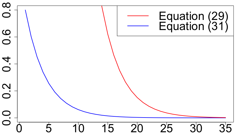
Figure 3: Behaviour of Equation 31 and Equation 29 as a function of $t$. We set $\eta=\frac{1}{2}$, $p=100$ and $t_{0}=100$. The starting distribution $\nu$ is randomly drawn from the $9$-dimensional simplex and the $10\times 10$ stochastic matrix is also obtained randomly. The spectral gap is computed exactly via numerical methods.

IV-C Concentration of measure without independence

Another application comes from leveraging Corollary 4 along with Equation 11 in proving concentration of measure bounds for non-independent random variables. In particular, the following result holds (see Section E-A for the proof).

Corollary 5.

For $i\geq 1$, let $K_{i}$ be a discrete-valued Markov kernel. Let $X_{1},\ldots,X_{t}$ be a sequence of random variables with joint measure $\mathcal{P}_{X^{t}}$ and marginals $\mathcal{P}_{X_{i}}$ with $1\leq i\leq t$. Assume that $\mathcal{P}_{X_{i}}=\mathcal{P}_{X_{i-1}}K_{i}$ i.e., the random variables are Markovian. Then, for every $p>1$ and every $f$ s.t. $|f(x)-f(\hat{x})|\leq\frac{1}{t}$ with $x$ and $\hat{x}$ two $t$-dimensional vectors differing only in the $i$-th position,

$$\mathbb{P}\left(\left\lvert f(X_{1},\ldots,X_{t})-\mathcal{P}_{\bigotimes_{i=1}^{t}X_{i}}(f)\right\rvert\geq\eta\right)\leq 2^{\frac{1}{q}}\exp\left(-\frac{2t\eta^{2}}{q}\right)\left(\prod_{i=2}^{t}\left(\left\lVert K_{i}^{\star}\right\rVert_{L_{p}^{0}\to L_{p}^{0}}\omega_{p}^{i}+1\right)\right),$$ (33)

where $\omega_{p}^{i}=\max_{x}((1-\mathcal{P}_{X_{i-1}}(\{x\}))^{p}\mathcal{P}_{X_{i-1}}(\{x\})^{1-p}$ $+(1-\mathcal{P}_{X_{i-1}}(\{x\})))^{\frac{1}{p}}$, and $\mathcal{P}_{\bigotimes_{i=1}^{t}X_{i}}(f)$ is the product of the marginals.

To compare with existing results, we start from a binary setting: $\mathcal{P}_{X_{i}|X_{i-1}}(0|0)=1-\lambda$ and $\mathcal{P}_{X_{i}|X_{i-1}}(1|1)=1-\kappa$ for every $i$ with $\kappa,\lambda<1$. This corresponds to the kernel $K_{\lambda,\kappa}$ induced by the matrix described in Example 2 in Appendix B. Let $\pi=1/(\kappa+\lambda)\cdot(\kappa,\lambda)$ denote the stationary distribution. Theorem 2 by [12] employs the hypercontractivity of the Markov operator $K_{\lambda,\kappa}$ to give a concentration result. Note that in this setting, the hypercontraction coefficient is not known, while the contraction coefficient can still be bounded via Equation 11 as

$$\left\lVert K_{\lambda,\kappa}^{\star}\right\rVert_{L_{p}^{0}\to L_{p}^{0}}\leq 2|1-\lambda-\kappa|,$$ (34)

which combined with Corollary 5 gives

$$\mathbb{P}\left(\left\lvert f(X_{1},\ldots,X_{t})-\mathcal{P}_{\bigotimes_{i=1}^{t}X_{i}}(f)\right\rvert\geq\eta\right)$$

$$\leq 2^{\frac{1}{q}}\exp\left(-\frac{2t\eta^{2}}{q}+(t-1)\log\left(2|1-\lambda-\kappa|\left(\left(\frac{\kappa}{\lambda}\right)^{p}\frac{\lambda}{\lambda+\kappa}+\frac{\kappa}{\lambda+\kappa}\right)^{\frac{1}{p}}+1\ \right)\right).$$ (35)

Assuming without loss of generality that $\kappa>\lambda$ and taking $p\to\infty$ leads to

$$\mathbb{P}\left(\left\lvert f(X_{1},\ldots,X_{t})-\mathcal{P}_{\bigotimes_{i=1}^{t}X_{i}}(f)\right\rvert\geq\eta\right)\leq 2\exp\left(-2t\eta^{2}+(t-1)\log\left(\frac{2|1-\lambda-\kappa|\kappa+\lambda}{\lambda}\ \right)\right).$$ (36)

One can then compute a similar bound leveraging Theorem 2 in [12] and then take the limit $p\to\infty$, which gives

$$\mathbb{P}\left(\left\lvert f(X_{1},\ldots,X_{t})-\mathcal{P}_{\bigotimes_{i=1}^{t}X_{i}}(f)\right\rvert\geq\eta\right)\leq 2\exp\left(-2t\eta^{2}+(t-1)\log\left(\frac{\lambda+\kappa}{\lambda}\ \right)\right).$$ (37)

Thus, the approach by [12] guarantees an exponential decay if

$$\eta>\sqrt{\frac{1}{2}\log\left(\frac{\kappa+\lambda}{\lambda}\right)(1+o_{t}(1))}.$$ (38)

In contrast, the approach provided here leads to the exponential concentration if (see Equation 36)

$$\eta>\sqrt{\frac{1}{2}\log\left(\frac{2|1-\lambda-\kappa|\kappa+\lambda}{\lambda}\right)(1+o_{t}(1))}.$$ (39)

Hence, Equation 36 improves over Equation 37 if $2|1-\lambda-\kappa|<1$, i.e., if the bound on the contraction coefficient in Equation 34 is less than $1$. Notably, if $\lambda=\kappa$, then Equation 11 leads to the same bound as [12, Equation (110)], with the main difference that [12] explicitly compute the required norms while in this work we exploit our novel bound on the contraction coefficient and still achieve the same result.

Similarly, for arbitrary $m\times m$ doubly-stochastic matrices, Corollary 5 with $p\to\infty$ improves over [12] whenever the bound on the contraction coefficient is less than $1$, see Section E-B for details. Furthermore, for $m\times m$ stochastic matrices, we now compare Corollary 5 with the approach by [12] via numerical experiments. In particular, selecting $\mathcal{P}_{X_{0}}$ as the stationary distribution, [12] prove exponential concentration if

$$\eta>\eta_{1}=\sqrt{(1+o_{t}(1))\ln(m)/2}.$$

In contrast, Corollary 5 leads to exponential concentration if

$$\eta>\eta_{2}=\sqrt{q(1+o_{t}(1))\ln(\left\lVert K^{\star}\right\rVert_{L_{p}^{0}\to L_{p}^{0}}\omega_{p}+1))/2},$$

with $\omega_{p}=\omega_{p}^{1}$ as defined in Corollary 5. In Figure 4a and Figure 4b, we compare the two bounds for a $5\times 5$ randomly generated stochastic matrix when: (a) $\eta_{2}<\eta<\eta_{1}$, and (b) $\eta>\eta_{1}>\eta_{2}$. In the first case, [12] cannot provide exponential concentration, and the improvement brought by Corollary 5 is obvious. In the second case, even if both approaches lead to exponential concentration, Corollary 5 is still better for intermediate values of $t$.

Figure 4: Behaviour of Corollary 5 and [12, Thm 1], as a function of $t$, for $p=100$ and two different choices of $\eta$.

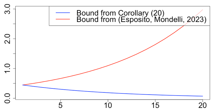
(a) $\eta=\eta_{2}+0.1$

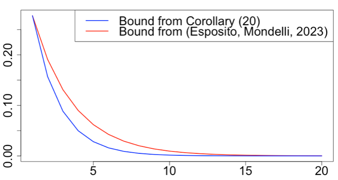
(b) $\eta=\eta_{1}+0.1$

V Conclusions

The notion of convergence of a Markov process induced by a kernel $K$ in Orlicz spaces is introduced. We show that one can control the speed of said convergence by studying the contraction coefficient of the dual kernel $K^{\star}$. Specifically, by considering specific norms of densities of $K$ and $K^{\star}$, Theorem 3 provides a novel and closed-form bound on the contraction coefficient in any Orlicz space. As discussed in Section IV, this yields a vast improvement over the state of the art in error bounds on MCMC methods, as well as in the concentration of Markovian processes. Given the generality of the framework, as explained in Remark 3, our analysis is able to tackle under-explored settings, such as those involving heavy-tailed distributions.

We envision applications of the results brought forth to other settings of interest. For instance, multi-armed bandit problems with Markovian rewards represent a severely under-studied setting in the literature [23]. The reason is that bandit algorithms heavily rely on concentration results. Hence, the improvements provided for the concentration of Markovian random variables can impact the development of bandit algorithms. Another setting comes from information theory: data-processing inequalities (DPI) are fundamental results in the field, and they can be significantly improved by computing the strong DPI (SDPI) constant for divergences [13]. Some connections between contraction coefficients of Markov kernels and strong DPI constants already exist [24, 16, 13]. Hence, leveraging Theorem 3 for $L_{\psi}$ spaces, one can also provide improved bounds on SDPI constants for $\psi$-divergences.

Appendix A Additional preliminaries and results

A-A Orlicz spaces

Orlicz spaces are quite general, and they include the well-known $L_{p}$-spaces. Indeed, if $\psi(x)=|x|^{p}$, then $L_{\psi}=L_{p}$ and $\left\lVert\cdot\right\rVert_{L^{L}_{\psi}(\mu)}$ is the $L^{p}$-norm, see Equation 5. We note that different choices of $\psi$ categorize different tail behaviors of random variables.

Example 1.

Let $\psi(x)=e^{x^{2}}-1$ and, given a measure space $(\Omega,\mathcal{F},\mu)$, define on $(\Omega,\mathcal{F})$ the Orlicz space $L_{\psi}(\mu)$. Given a random variable $X$ defined on this space, $\left\lVert X\right\rVert_{\psi,\mu}$ is the sub-Gaussian norm, i.e.,

$$\left\lVert X\right\rVert_{L^{L}_{\psi}(\mu)}=\inf\left\{\sigma>0:\mu\left(\exp\left(\frac{X^{2}}{\sigma^{2}}\right)\right)\leq 2\right\}.$$ (40)

Thus, $L_{\psi}(\mu)$ represents the set of all sub-gaussian random variables with respect to $\mu$ [25, Definition 2.5.6].

Given a function and its Young’s dual, the following generalised Hölder’s inequality holds, see [26, Appendix A] for a proof.

Lemma 2.

Let $\psi$ be an Orlicz function and $\psi^{\star}$ its complementary function. For every pair of non-negative random variables $U,V$ respectively defined over $(\Omega_{U},\mathcal{F}_{U},\mathcal{P}_{U}),(\Omega_{V},\mathcal{F}_{V},\mathcal{P}_{V})$, given a coupling $\mathcal{P}_{UV}(UV)$, one has that

$$\mathcal{P}_{UV}(UV)\leq\lVert U\rVert_{L^{L}_{\psi}(\mathcal{P}_{U})}\lVert V\rVert_{L^{A}_{\psi^{\star}}(\mathcal{P}_{V})}.$$ (41)

Choosing $\psi(x)=|x|^{p}$, which implies ${\psi}^{\star}(x^{\star})=|x^{\star}|^{q}\frac{(p-1)}{p^{q}}$ with $\frac{1}{p}+\frac{1}{q}=1$, Lemma 2 yields the classical Hölder’s inequality:

$$\mathcal{P}_{UV}(UV)\leq\left\lVert U\right\rVert_{L^{p}(\mathcal{P}_{U})}\cdot\left\lVert V\right\rVert_{L^{q}(\mathcal{P}_{V})}.$$ (42)

A-B Proof of Lemma 1

Proof.

Given that $\nu\ll\mu$, one has that $\nu K\ll\mu K$. Indeed, let $E$ be an event such that $\mu K(E)=0$. Then,

$$\mu K(E)=\int\mathbbm{1}_{E}d\mu K=\int K(\mathbbm{1}_{E})d\mu=0.$$ (43)

Hence, $K(\mathbbm{1}_{E})$ is $0$ $\mu$-a.e., and by absolute continuity between $\nu$ and $\mu$, $K(\mathbbm{1}_{E})$ is also $0$ $\nu$-a.e. and $\nu K(E)=0$. Thus, the function $g$ is well-defined. Moreover, given any function $h$,

$$\langle h,g\rangle_{\mu K}=\mu K(h\cdot g) =\int h\frac{d\nu K}{d\mu K}d\mu K$$ (44)

$$=\int hd\nu K$$ (45)

$$=\int Khd\nu$$ (46)

$$=\int(Kh)fd\mu=\langle Kh,f\rangle_{\mu}=\langle h,K^{\star}_{\mu}f\rangle_{\mu K},$$ (47)

which implies that $g=K^{\star}_{\mu}f$, $\mu K$-almost everywhere. ∎

An important result allows us to characterise the contraction coefficient of the $t$-fold application $K^{t}$ of a Markovian operator, leveraging the contraction coefficient of $K$ itself.

Theorem 5.

Let $K$ be a Markov kernel reversible with respect to $\pi$, and let $\psi$ be a Young functional. Then, for every $f\in L_{\psi}^{0}(\pi)$ and for every $t\in\mathbb{N}$, we have

$$\left\lVert K^{t}f\right\rVert_{L_{\psi}^{N}(\pi)}\leq\left\lVert K\right\rVert_{L_{\psi}^{N,0}\to L_{\psi}^{N,0}}\cdot\left\lVert K^{t-1}f\right\rVert_{L_{\psi}^{N}(\pi)}.$$ (48)

Consequently, one has that:

$$\left\lVert K^{t}\right\rVert_{L_{\psi}^{N,0}\to L_{\psi}^{N,0}}\leq\left\lVert K\right\rVert_{L_{\psi}^{N,0}\to L_{\psi}^{N,0}}^{t}.$$ (49)

Proof.

For a given $x$ and measurable event $E$, $K^{t}(E|x)=\int K^{t-1}(E|z)dK(z|x)$ and consequently $K^{t}f=Kg$ $\pi$-a.e., where $g(z)=K^{t-1}f(z)$. Indeed, it follows by Fubini’s theorem that

$$K^{t}f(x)=\int_{y}f(y)dK^{t}(y|x) =\int_{y}f(y)\int_{z}K^{t-1}(y|z)dK(z|x)$$ (50)

$$=\int_{z}dK(z|x)\int_{y}f(y)K^{t-1}(y|z)$$ (51)

$$=\int_{z}dK(z|x)K^{t-1}f(z)=Kg(x).$$ (52)

Hence, one can conclude that

$$\left\lVert K^{t}f\right\rVert_{L_{\psi}^{N}(\pi)}=\left\lVert Kg\right\rVert_{L_{\psi}^{N}(\pi)}\leq\left\lVert K\right\rVert_{L_{\psi}^{N,0}\to L_{\psi}^{N,0}}\cdot\left\lVert g\right\rVert_{L_{\psi}^{N}(\pi)}=\left\lVert K\right\rVert_{L_{\psi}^{N,0}\to L_{\psi}^{N,0}}\cdot\left\lVert K^{t-1}f\right\rVert_{L_{\psi}^{N}(\pi)},$$ (53)

where the inequality in Equation 53 follows from the fact that $g\in L_{\psi}^{0}(\pi)$. Indeed, $\pi(g)=\int gd\pi=\int K^{t-1}fd\pi=\int fd(\pi K^{t-1})=\int fd\pi=0$, as $f\in L_{\psi}^{0}(\pi).$ ∎

A-C Relationship between contraction coefficients

Theorem 6.

Let $\psi$ be a Young functional, $N\in\{A,L\}$ and let $t\in\mathbb{N}$. Then, the following holds:

$$\left\lVert K^{t}\right\rVert_{L_{\psi}^{N,0}\to L_{\psi}^{N,0}} \leq\left\lVert(K-1_{\pi})^{t}\right\rVert_{L_{\psi}^{N}\to L_{\psi}^{N}}\leq 2\left\lVert K^{t}\right\rVert_{L_{\psi}^{N,0}\to L_{\psi}^{N,0}}.$$ (54)

Remark 4.

Taking $\psi(x)=|x|^{p}$, which gives $L_{p}$-norms, we recover Lemma 3.16 by [2].

Proof.

The first inequality is obtained via the passages below:

$$\left\lVert K^{t}\right\rVert_{L_{\psi}^{N,0}\to L_{\psi}^{N,0}} =\sup_{g:\left\lVert g\right\rVert_{L_{\psi}^{N}(\pi)}\leq 1,\pi(g)=0}\left\lVert K^{t}g\right\rVert_{L_{\psi}^{N}(\pi)}$$ (55)

$$=\sup_{g:\left\lVert g\right\rVert_{L_{\psi}^{N}(\pi)}\leq 1,\pi(g)=0}\left\lVert(K^{t}-1_{\pi})g\right\rVert_{L_{\psi}^{N}(\pi)}$$ (56)

$$\leq\sup_{f:\left\lVert f\right\rVert_{L_{\psi}^{N}(\pi)}\leq 1,}\left\lVert(K^{t}-1_{\pi})f\right\rVert_{L_{\psi}^{N}(\pi)}$$ (57)

$$=\left\lVert K^{t}-1_{\pi}\right\rVert_{L_{\psi}^{N}\to L_{\psi}^{N}}.$$ (58)

Moreover, one has that there exists a constant $c_{N}$ such that the following sequence of steps holds:

$$\left\lVert K^{t}-1_{\pi}\right\rVert_{L_{\psi}^{N}\to L_{\psi}^{N}} =\sup_{f:\left\lVert f\right\rVert_{L_{\psi}^{N}(\pi)}\leq 1}\left\lVert(K^{t}-1_{\pi})f\right\rVert_{L_{\psi}^{N}(\pi)}$$ (59)

$$=\sup_{f:\left\lVert f\right\rVert_{L_{\psi}^{N}(\pi)}\leq 1}\left\lVert K^{t}(f-\pi(f))\right\rVert_{L_{\psi}^{N}(\pi)}$$ (60)

$$=c_{N}\sup_{f:\left\lVert f\right\rVert_{L_{\psi}^{N}(\pi)}\leq 1}\left\lVert K^{t}\left(\frac{f-\pi(f)}{c_{N}}\right)\right\rVert_{L_{\psi}^{N}(\pi)}$$ (61)

$$\leq c_{N}\sup_{g:\left\lVert g\right\rVert_{L_{\psi}^{N}(\pi)}\leq 1,\pi(g)=0}\left\lVert K^{t}g\right\rVert_{L_{\psi}^{N}(\pi)}$$ (62)

$$=c_{N}\left\lVert K^{t}\right\rVert_{L_{\psi}^{N,0}\to L_{\psi}^{N,0}}.$$ (63)

It remains to upper bound the constant $c_{N}$. In order for Equation 62 to hold, $c_{N}$ needs to satisfy

$$\left\lVert\frac{f-\pi(f)}{c_{N}}\right\rVert_{L^{N}_{\psi}(\pi)}\leq 1.$$

One clearly has that

$$\left\lVert\frac{f-\pi(f)}{c_{N}}\right\rVert_{L^{N}_{\psi}(\pi)}\leq\frac{1}{|c_{N}|}\left(\left\lVert f\right\rVert_{L^{N}_{\psi}(\pi)}+\left\lVert\pi(f)\right\rVert_{L^{N}_{\psi}(\pi)}\right).$$ (64)

In particular, an application of Jensen’s inequality gives

$$\left\lVert\pi(f)\right\rVert_{L_{\psi}^{N}(\pi)}\leq\pi(\left\lVert f\right\rVert_{L_{\psi}^{N}(\pi)})\leq 1.$$ (65)

This gives the upper bound $c_{N}\leq 2$ and concludes the proof. ∎

To conclude our characterisation of the contraction coefficients, we prove the equivalence between $\left\lVert(K-1_{\pi})^{\star}\right\rVert_{L_{\psi}^{N}\to L_{\psi}^{N}}$ and $\left\lVert K^{\star}-1_{\pi}\right\rVert_{L_{\psi}^{N}\to L_{\psi}^{N}}$.

Lemma 3.

Let $K$ be a Markov kernel with stationary distribution $\pi$, and $K^{\star}=K^{\star}_{\pi}$ the dual kernel. Then, one has that

$$(K-1_{\pi})^{\star}=K^{\star}-1_{\pi},\pi-a.e.$$ (66)

Proof.

We first show that $1_{\pi}^{\star}=1_{\pi}$, i.e., that for every function $h$ and $f$, $\langle 1_{\pi}h,f\rangle_{\pi}=\langle h,1_{\pi}f\rangle_{\pi}$. Indeed, we have

$$\langle 1_{\pi}h,f\rangle_{\pi}=\int d\pi f\pi(h)=\pi(f)\pi(h)=\int d\pi h\pi(f)=\langle h,1_{\pi}f\rangle_{\pi}.$$ (67)

From this, one can also conclude that, if $K$ is stationary with respect to $\pi$, then $(K-1_{\pi})^{\star}=K^{\star}-1_{\pi}$. Indeed, we have

$$\langle(K-1_{\pi})h,f\rangle_{\pi}=\langle Kh,f\rangle_{\pi}-\langle 1_{\pi}h,f\rangle_{\pi}=\langle h,K^{\star}f\rangle_{\pi}-\langle h,1_{\pi}f\rangle_{\pi}=\langle h,(K^{\star}-1_{\pi})f\rangle_{\pi}.$$ (68)

∎

Appendix B Examples: discrete-valued kernels

Example 2.

Consider a binary setting where the Markov kernel is induced by a $2\times 2$ matrix:

$$K_{\lambda,\kappa}=\begin{bmatrix}1-\lambda&\lambda\\ \kappa&1-\kappa\end{bmatrix}.$$ (69)

In this case, the stationary distribution is $\pi=\frac{1}{\kappa+\lambda}(\kappa,\lambda)$, and the dual kernel is $K^{\star}_{\lambda,\kappa}=K^{T}_{\lambda,\kappa}$. If $\kappa=\lambda$, we use the shorthands $K_{\lambda}$ and $K^{\star}_{\lambda}$ to denote $K_{\lambda,\lambda}$ and $K^{\star}_{\lambda,\lambda}$, respectively. We note that $K_{\lambda}$ is known in information theory as the binary symmetric channel with parameter $\lambda$. Now, both $K_{\lambda}$ and $K^{\star}_{\lambda}$ are doubly-stochastic and the stationary distribution is $\pi=\left(\frac{1}{2},\frac{1}{2}\right)$.

Let us focus on the setting where $\psi(x)=|x|^{2}$, in which we can compute everything explicitly and thus compare the upper bound to the real quantity. In this case, $\left\lVert K_{\lambda,\kappa}\right\rVert_{L_{2}^{0}\to L_{2}^{0}}=\gamma$ is ($1$ minus) the spectral gap i.e., the second largest singular value of $K_{\lambda,\kappa}^{\star}$. Thus, $\gamma=|1-\lambda-\kappa|$. Let us now compute the bound on $\left\lVert K_{\lambda,\kappa}\right\rVert_{L_{2}^{0}\to L_{2}^{0}}$ that stems from Equation 11. In particular, one has that

$$\begin{split}g_{0}(0)&=\frac{(1-\lambda)(\lambda+\kappa)}{\kappa},\\ g_{0}(1)&=g_{1}(0)=\kappa+\lambda,\\ g_{1}(1)&=\frac{(1-\kappa)(\lambda+\kappa)}{\lambda}.\end{split}$$

Consequently,

$$|1-\lambda-\kappa|=\left\lVert K_{\lambda,\kappa}\right\rVert_{L_{2}^{0}\to L_{2}^{0}} \leq\left|\sum_{x}\left|\sum_{y}\left|g_{x}(y)-1\right|^{2}\pi(\{y\})\right|\pi(\{x\})\right|^{\frac{1}{2}}=|1-\lambda-\kappa|.$$ (70)

In a $3\times 3$ example, the bound is still very close to the actual value. Specifically, we consider the following matrix:

$$\Lambda=\begin{bmatrix}0.2&0.1&0.7\\ 0.3&0.4&0.3\\ 0.5&0.5&0\end{bmatrix}.$$ (71)

Given that $\Lambda$ is doubly-stochastic, the stationary distribution $\pi$ is uniform, i.e., $\pi(\{x\})=1/3$ for $x\in\{0,1,2\}$. Similarly to the $2\times 2$ setting, $\Lambda^{\star}=\Lambda^{T}$. We can thus numerically compute the second largest singular value of $\Lambda^{T}$ which gives $\gamma=\left\lVert\Lambda\right\rVert_{L_{2}^{0}\to L_{2}^{0}}$. Instead, Equation 11 leads to the bound below which is very close to the actual value of $\gamma$:

$$0.61098529=\gamma\leq\left\lVert\left\lVert g_{X}-1\right\rVert_{L_{2}(\pi)}\right\rVert_{L_{2}(\pi)}=0.6164414.$$ (72)

More generally, one can prove the following.

Lemma 4.

Consider a discrete-valued Markovian process described by an $m\times m$ doubly-stochastic matrix $\Lambda\in[0,1]^{m\times m}$. Then, the contraction coefficient of $\Lambda$ in the space $L_{p}^{0}$ can be bounded as follows:

$$\left\lVert\Lambda^{T}\right\rVert_{L_{p}^{0}\to L_{p}^{0}}\leq\left(\sum_{j}\left(\sum_{i}\left|\lambda_{j,i}-\frac{1}{m}\right|^{q}\right)^{\frac{p}{q}}\right)^{\frac{1}{p}}.$$ (73)

Proof.

The stationary distribution $\pi$ is the uniform distribution: $\pi(\{i\})=\frac{1}{m}$, for $1\leq i\leq m$. It is also easy to see that the dual of the kernel $K$ induced by $\Lambda$ with respect to $\pi$ is the transpose matrix $\Lambda^{\star}_{\pi}=\Lambda^{T}$. By using Equation 11, we can write

$$\left\lVert\Lambda^{T}\right\rVert_{L_{p}^{0}\to L_{p}^{0}}^{p} \leq\sum_{j}\frac{1}{m}\left(\sum_{i}\frac{1}{m}|m\lambda_{j,i}-1|^{q}\right)^{\frac{p}{q}}$$ (74)

$$=m^{\frac{p(q-1)}{q}-1}\sum_{j}\left(\sum_{i}\left|\lambda_{j,i}-\frac{1}{m}\right|^{q}\right)^{\frac{p}{q}}=\sum_{j}\left(\sum_{i}\left|\lambda_{j,i}-\frac{1}{m}\right|^{q}\right)^{\frac{p}{q}},$$ (75)

which concludes the proof. ∎

In the case of general $m\times m$ doubly-stochastic matrices, we can see that the bound maintains some of its properties but not all. For instance, it is still true that, if the matrix enforces independence (i.e., $\lambda_{i,j}=\frac{1}{m}$ for every $i,j$), then $\left\lVert\Lambda^{T}\right\rVert_{L_{p}^{0}\to L_{p}^{0}}\leq 0$. However, it is not always true that the bound on the contraction coefficient is always strictly less than one. Indeed, if $\Lambda$ is deterministic (i.e., for every $j$ there exists an $i$ such that $\lambda_{i,j}=1$ and $\lambda_{k,j}=0$ for every $k\neq i$), one can see that the bound becomes:

$$\left\lVert\Lambda^{T}\right\rVert_{L_{p}^{0}\to L_{p}^{0}}^{p}\leq((m-1)^{q}+(m-1))^{\frac{p}{q}}m^{1-p},$$ (76)

which is larger than $1$ for $m>2$ and $p\geq 1$.

Appendix C Proofs for Section III

C-A Proof of Theorem 1

Assume that, for every $\epsilon>0$, there exists a constant $\lambda$ such that

$$\lambda=\left\lVert f\right\rVert_{L^{L}_{\psi}(\pi)}+\epsilon\hskip 20.00003pt\text{and}\hskip 20.00003pt\pi\left(\psi\left(\frac{|f|}{\lambda}\right)\right)\leq 1.$$ (77)

Moreover, the following steps hold:

$$\pi\left(\psi\left(\frac{|Kf|}{\lambda}\right)\right) \leq\pi\left(\psi\left(\frac{K|f|}{\lambda}\right)\right)$$ (78)

$$\leq K\pi\left(\psi\left(\frac{|f|}{\lambda}\right)\right)$$ (79)

$$=\pi\left(\psi\left(\frac{|f|}{\lambda}\right)\right)\leq 1.$$ (80)

Hence, since $\left\lVert Kf\right\rVert_{L_{\psi}^{L}(\pi)}=\inf\left\{\sigma>0:\pi\left(\psi\left(\frac{|Kf|}{\sigma}\right)\right)\leq 1\right\}$ one has that $\left\lVert Kf\right\rVert_{L_{\psi}^{L}(\pi)}\leq\lambda=\left\lVert f\right\rVert_{L_{\psi}^{L}(\pi)}+\epsilon$. The statement follows from the arbitrariness of $\epsilon$. To conclude the argument for the Luxemburg norm, select the function $g$ identically equal to $\psi^{-1}(1)>0$. One has that in order for $\pi\left(\left(\frac{g}{\lambda}\right)\right)=\pi\left(\psi\left(\frac{\psi^{-1}(1)}{\lambda}\right)\right)\leq 1$ the following needs to hold

$$\lambda\geq\frac{\psi^{-1}(1)}{\psi^{-1}(1)}=1,$$ (81)

and thus $\left\lVert g\right\rVert_{L^{L}_{\psi}(\pi)}=1$. Hence, since $Kg=g$, one has that $\left\lVert K\right\rVert_{L_{\psi}^{L}\to L_{\psi}^{L}}=1$.

As for the Amemiya norm, assume that, for every $\epsilon>0$, there exists $\lambda$ such that

$$\frac{1+\pi(\psi(\lambda|f|))}{\lambda}\leq\left\lVert f\right\rVert_{L^{A}_{\psi}(\pi)}+\epsilon,$$ (82)

then one has that for every Markov kernel $K$

$$\left\lVert Kf\right\rVert_{L^{A}_{\psi}(\pi)}\leq\frac{1+\pi(\psi(\lambda|Kf|))}{\lambda} \leq\frac{1+\pi(\psi(\lambda K|f|))}{\lambda}$$ (83)

$$\leq\frac{1+K\pi(\psi(\lambda|f|))}{\lambda}$$ (84)

$$=\frac{1+\pi(\psi(\lambda|f|))}{\lambda}$$ (85)

$$\leq\left\lVert f\right\rVert_{L^{A}_{\psi}(\pi)}+\epsilon.$$ (86)

The argument then follows from the arbitrariness of $\epsilon$. This implies that $\left\lVert K\right\rVert_{L_{\psi}^{A}\to L_{\psi}^{A}}\leq 1$. Moreover, if one selects $g$ to be the function identically equal to $\frac{1}{{\psi^{\star}}^{-1}(1)}$, then

$$\left\lVert g\right\rVert_{L^{A}_{\psi}(\pi)}=\inf_{t>0}\frac{1+\pi\left(\psi\left(\frac{t}{{\psi^{\star}}^{-1}(1)}\right)\right)}{t} =\inf_{t>0}\frac{1+\psi\left(\frac{t}{{\psi^{\star}}^{-1}(1)}\right)}{t}=1.$$ (87)

Indeed, denoting $\varphi(x)=\psi(x/{\psi^{\star}}^{-1}(1))$, one has that $\varphi^{\star}(x)=\psi^{\star}(x{\psi^{\star}}^{-1}(1))$ and ${\varphi^{\star}}^{-1}(y)={\psi^{\star}}^{-1}(y)/{\psi^{\star}}^{-1}(1)$. Given that

$$\inf_{t>0}\frac{1+\psi\left(\frac{t}{{\psi^{\star}}^{-1}(1)}\right)}{t}=\inf_{t>0}\frac{1+\varphi(t)}{t}={\varphi^{\star}}^{-1}(1)=\frac{{\psi^{\star}}^{-1}(1)}{{\psi^{\star}}^{-1}(1)},$$ (88)

the argument follows. Hence, similarly to before, since $Kg=g$, one has that $\left\lVert K\right\rVert_{L_{\psi}^{A}\to L_{\psi}^{A}}=1$.

C-B Proof of Theorem 2

Let $t\in\mathbb{N}$ and let $\nu\ll\pi$. Then,

$$\left\lVert\frac{d\nu K^{t}}{d\pi}-1\right\rVert_{L_{\psi}^{N}(\pi)} =\left\lVert\frac{d\nu K^{t}}{d\pi K^{t}}-1\right\rVert_{L_{\psi}^{N}(\pi)}$$ (89)

$$=\left\lVert{K^{t}}^{\star}\frac{d\nu}{d\pi}-1\right\rVert_{L_{\psi}^{N}(\pi)}$$ (90)

$$=\left\lVert{K^{t}}^{\star}\left(\frac{d\nu}{d\pi}-1\right)\right\rVert_{L_{\psi}^{N}(\pi)}$$ (91)

$$\leq\left\lVert{K^{t}}^{\star}\right\rVert_{L_{\psi}^{N,0}\to L_{\psi}^{N,0}}\left\lVert\frac{d\nu}{d\pi}-1\right\rVert_{L_{\psi}^{N}(\pi)}$$ (92)

$$\leq\left\lVert{K}^{\star}\right\rVert_{L_{\psi}^{N,0}\to L_{\psi}^{N,0}}^{t}\left\lVert\frac{d\nu}{d\pi}-1\right\rVert_{L_{\psi}^{N}(\pi)},$$ (93)

where Equation 92 follows by the definition of $\left\lVert{K}^{\star}\right\rVert_{L_{\psi}^{N,0}\to L_{\psi}^{N,0}}$ (see Definition 4) and the fact that if $f=\frac{d\nu}{d\pi}-1$ then $\pi\left(f\right)=0$; Equation 93 follows from Theorem 5.

C-C Proof of Theorem 3

As $f\in L_{\psi}^{0}(\mu K)$, we have that $\mu(f)=0$. Thus,

$$\left\lVert Kf\right\rVert_{L_{\psi}^{N}(\mu)} =\left\lVert|Kf|\right\rVert_{L_{\psi}^{N}(\mu)}$$ (94)

$$=\left\lVert\left|\int f(y)dK(y|X)\right|\right\rVert_{L_{\psi}^{N}(\mu)}$$ (95)

$$=\left\lVert\left|\int g_{X}(y)f(y)d\mu K\right|\right\rVert_{L_{\psi}^{N}(\mu)}$$ (96)

$$=\left\lVert\left|\int(g_{X}(y)-1)f(y)d\mu K\right|\right\rVert_{L_{\psi}^{N}(\mu)}$$ (97)

$$\leq\left\lVert\int\left|(g_{X}(y)-1)f(y)\right|d\mu K\right\rVert_{L_{\psi}^{N}(\mu)}$$ (98)

$$\leq\left\lVert f\right\rVert_{L_{\psi}^{N}(\mu K)}\left\lVert\left\lVert g_{X}-1\right\rVert_{L_{\psi}^{N^{\star}}(\mu K)}\right\rVert_{L_{\psi}^{N}(\mu)},$$ (99)

where Equation 94 follows from the fact that Amemiya and Luxemburg norms are “ideal norms”, Equation 98 follows from the fact that $\mu K$ is a probability measure along with Jensen’s inequality, and Equation 99 follows from generalised Hölder’s inequality, i.e., Lemma 2. This gives the desired bound on the contraction coefficient of $K$. The bound on the contraction coefficient of $K^{\star}$ follows from an analogous argument.

C-D Proof of Corollary 1

The inequality follows from Equation 11 with $p\to\infty$. As for the equality, notice that, for every $x$, and $t\in\mathbb{N}$

$$\left\lVert g^{t}_{x}-1\right\rVert_{L_{1}(\pi)}=\left\lVert\frac{dK^{t}(Y|x)}{d\pi(Y)}-1\right\rVert_{L_{1}(\pi)} =\int d\pi(y)\left|\frac{dK^{t}(y|x)}{d\pi(y)}-1\right|$$ (100)

$$=2\left\lVert K^{t}(\cdot|x)-\pi\right\rVert_{TV}.$$ (101)

The last step follows from the definition of Total Variation distance. Hence,

$$\left\lVert\left\lVert g^{t}_{X}-1\right\rVert_{L_{1}(\pi)}\right\rVert_{L_{q}(\pi)}\xrightarrow[q\to\infty]{}\operatorname*{ess\,sup}_{\pi}\left\lVert g^{t}_{X}-1\right\rVert_{L_{1}(\pi)}=\operatorname*{ess\,sup}_{\pi}2\left\lVert K^{t}(\cdot|X)-\pi\right\rVert_{TV}.$$ (102)

C-E Proof of Corollary 2

In [16, Lemma 4.1], the authors prove that if Equation 13 holds, then for every measure $\xi$ one has that:

$$\frac{dK_{\xi}^{\star}(\cdot|Y)}{d\xi}\geq\epsilon\hskip 20.00003pt\xi K-a.e.,$$ (103)

where $Y$ is distributed according to $\xi K$. Given that $0<\epsilon<1$ and selecting $\xi=\mu$, this implies that $g_{Y}(x)\geq\epsilon$ for every $x$ and $\mu K$-a.e.; thus, for every $y$ and $x$, $|g_{y}(x)-1|\leq|\epsilon-1|=(1-\epsilon).$ Note that norms are non-decreasing and

$$\left\lVert\left\lVert c\right\rVert_{L_{\psi^{\star}}^{L}(\mu)}\right\rVert_{L_{\psi}^{A}(\mu K)}=\left\lVert\frac{|c|}{{\psi^{\star}}^{-1}(1)}\right\rVert_{L_{\psi}^{A}(\mu)}=\frac{|c|{\psi^{\star}}^{-1}(1)}{{\psi^{\star}}^{-1}(1)}=|c|=\left\lVert\left\lVert c\right\rVert_{L_{\psi^{\star}}^{A}(\mu K)}\right\rVert_{L_{\psi}^{L}(\mu K)}.$$

Then, the claim follows from an application of Theorem 2 with $t=1$ and Theorem 3.

Appendix D Proofs for Section IV-A

D-A Computations for Remark 2

The following closed-form expressions for $\max_{x}\left\lVert\frac{d\delta_{x}}{d\pi}-1\right\rVert_{L_{\psi}^{N}(\pi)}$ hold:

$$\max_{x}\left\lVert\frac{d\delta_{x}}{d\pi}-1\right\rVert_{L_{\psi}^{L}(\pi)}\leq\max_{x}\begin{cases}1/{\psi}^{-1}\left(\frac{1}{2\pi(\Omega\setminus\{x\})}\right)&\text{ if }\pi(\{x\})\geq 1/2,\\ \frac{\pi(\Omega\setminus\{x\})}{\pi(\{x\})}\cdot 1/{\psi}^{-1}\left(\frac{1}{2\pi(\{x\})}\right)&\text{ else },\end{cases}$$ (104)

$$\max_{x}\left\lVert\frac{d\delta_{x}}{d\pi}-1\right\rVert_{L_{\psi}^{A}(\pi)}\leq 2\max_{x}\pi(\Omega\setminus\{x\})\begin{cases}{\psi^{\star}}^{-1}\left(\frac{1}{2\pi(\Omega\setminus\{x\})}\right)&\text{ if }\pi(\{x\})\geq 1/2,\\ {\psi^{\star}}^{-1}\left(\frac{1}{2\pi(\{x\})}\right)&\text{ else },\end{cases}$$ (105)

where $\Omega$ is the space over which $\nu$ and $\pi$ are defined and $\psi^{\star}$ the Young conjugate, see Equation 4. We start by proving Equation 104. Let $x$ be fixed. Then, for a given $\psi$ and $\sigma>0$,

$$\pi\left(\psi\left(\frac{\left|\frac{d\delta_{x}}{d\pi}-1\right|}{\sigma}\right)\right)=\pi(\{x\})\psi\left(\frac{\pi(\Omega\setminus\{x\})}{\pi(\{x\})}\frac{1}{\sigma}\right)+\pi(\Omega\setminus\{x\})\psi\left(\frac{1}{\sigma}\right).$$ (106)

We need to consider two cases. First assume that $\pi(\Omega\setminus\{x\})/\pi(\{x\})\leq 1$, which is equivalent to $\pi(\{x\})\geq 1/2$. Then, since $\psi$ is convex and $\psi(0)=0$, one has that

$$\pi(\{x\})\psi\left(\frac{\pi(\Omega\setminus\{x\})}{\pi(\{x\})}\frac{1}{\sigma}\right)+\pi(\Omega\setminus\{x\})\psi\left(\frac{1}{\sigma}\right)\leq 2\pi(\Omega\setminus\{x\})\psi\left(\frac{1}{\sigma}\right).$$ (107)

Thus, in order to have the right-hand side of Equation 107 less than one, one needs

$$\sigma\geq\frac{1}{\psi^{-1}\left(\frac{1}{2\pi(\Omega\setminus\{x\})}\right)}.$$

If instead $\pi(\Omega\setminus\{x\})/\pi(\{x\})\geq 1$, then

$$\pi(\{x\})\psi\left(\frac{\pi(\Omega\setminus\{x\})}{\pi(\{x\})}\frac{1}{\sigma}\right)+\pi(\Omega\setminus\{x\})\psi\left(\frac{1}{\sigma}\right)\leq 2\pi(\{x\})\psi\left(\frac{\pi(\Omega\setminus\{x\})}{\pi(\{x\})}\frac{1}{\sigma}\right).$$ (108)

Consequently, one needs

$$\sigma\geq\frac{\pi(\Omega\setminus\{x\})}{\pi(\{x\})\psi^{-1}\left(\frac{1}{2\pi(\{x\})}\right)}.$$

Analogous considerations allow us to derive a bound on the Amemiya norm. Indeed, if $\pi(\Omega\setminus\{x\})/\pi(\{x\})\leq 1$, then

$$\inf_{t>0}\frac{1+\pi\left(\psi\left(t\left|\frac{d\delta_{x}}{d\pi}-1\right|\right)\right)}{t} \leq\inf_{t>0}\frac{1+2\pi(\Omega\setminus\{x\})\psi(t)}{t}=2\pi(\Omega\setminus\{x\}){\psi^{\star}}^{-1}\left(\frac{1}{2\pi(\Omega\setminus\{x\})}\right).$$ (109)

One can then also similarly bound the Amemiya norm when $\pi(\Omega\setminus\{x\})/\pi(\{x\})\geq 1$.

D-B Proof of Theorem 4

The proof leverages the generalised Hölder’s inequality. Let $\mu K^{t}$ be the measure obtained in the Markovian process when $\mu$ is the starting distribution and after $t$ applications of the Markov kernel $K$. Assume that $\mu K^{t}\ll\pi$, with $\pi$ being the stationary distribution. The following sequence of steps hold for every Young function $\psi$:

$$\mu K^{t}(E)=\int_{E}d\mu K^{t} =\int\mathbbm{1}_{E}d\mu K^{t}$$ (110)

$$=\int\mathbbm{1}_{E}\frac{d\mu K^{t}}{d\pi}d\pi$$ (111)

$$=\left\langle\mathbbm{1}_{E},\frac{d\mu K^{t}}{d\pi}\right\rangle_{\pi}$$ (112)

$$\leq\left\lVert\mathbbm{1}_{E}\right\rVert_{L_{{\psi}^{\star}}^{N}(\pi)}\left\lVert\frac{d\mu K^{t}}{d\pi}\right\rVert_{L_{\psi}^{N}(\pi)}$$ (113)

$$\leq\left\lVert\mathbbm{1}_{E}\right\rVert_{L_{{\psi}^{\star}}^{N}(\pi)}\left(\left\lVert\frac{d\mu K^{t}}{d\pi}-1\right\rVert_{L_{\psi}^{N}(\pi)}+\left\lVert 1\right\rVert_{L_{\psi}^{N}(\pi)}\right)$$ (114)

$$=\begin{cases}1/{\psi^{\star}}^{-1}(1/\pi(E))\left(\left\lVert\frac{d\mu K^{t}}{d\pi}-1\right\rVert_{L_{\psi}^{A}(\pi)}+{\psi^{\star}}^{-1}(1)\right)\\ \pi(E)\psi^{-1}(1/\pi(E))\left(\left\lVert\frac{d\mu K^{t}}{d\pi}-1\right\rVert_{L_{\psi}^{L}(\pi)}+1/\psi^{-1}(1)\right)\end{cases}.$$ (115)

D-C Proof of Corollary 4

Since we know the exact closed-form expression of the norm when $\psi(x)=|x|^{p}/p$, it is possible to prove a stronger result directly. Consider the function $\hat{\psi}(x)=|x-1|^{p}/p$. This is a convex function such that $\hat{\psi}(1)=0$ and is no longer a Young function. One can thus define a corresponding $f$-divergence [27] with $f(x)=\hat{\psi}(x)$. I.e., given two measures $\mu\ll\nu$,

$$D_{\hat{\psi}}(\mu\|\nu)=\int\hat{\psi}\left(\frac{d\mu}{d\nu}\right)d\nu=\frac{1}{p}\left(\left\lVert\frac{d\mu}{d\nu}-1\right\rVert_{L_{p}(\pi)}\right)^{p}.$$ (116)

As such, it will satisfy the data-processing inequality, which we can use to prove Corollary 4. Following the same steps undertaken to prove [26, Theorem 3], for every event $E$ one has that

$$\frac{D_{\hat{\psi}}(\mu\|\nu)+\nu(E^{c}){\hat{\psi}}^{\star}(0)}{\nu(E)}\geq\hat{\psi}\left(\frac{\mu(E)}{\nu(E)}\right).$$ (117)

If $\mu(E)\geq\nu(E)$, we can then invert $\hat{\psi}$ and obtain

$$\mu(E)\leq\nu(E)\hat{\psi}^{-1}\left(\frac{D_{\hat{\psi}}(\mu\|\nu)+\nu(E^{c}){\hat{\psi}}^{\star}(0)}{\nu(E)}\right).$$ (118)

Moreover, one has that $\hat{\psi}^{\star}(y)=|y|^{q}/q+y$, and thus $\hat{\psi}^{\star}(0)=0$. Hence, one can rewrite Equation 118 as follows:

$$\mu(E)\leq\nu(E)\left(\left(p\frac{D_{\hat{\psi}}(\mu\|\nu)}{\nu(E)}\right)^{\frac{1}{p}}+1\right)=\nu(E)+\nu(E)^{\frac{1}{q}}\left\lVert\frac{d\mu}{d\nu}-1\right\rVert_{L_{p}(\pi)}.$$ (119)

If $\mu(E)\leq\nu(E)$, then the claim holds trivially as $\nu(E)^{\frac{1}{q}}\left\lVert\frac{d\mu}{d\nu}-1\right\rVert_{L_{p}(\pi)}\geq 0$.

Appendix E Proofs for Section IV-C

E-A Proof of Corollary 5

From [12, Theorem 1], we have that

$$\frac{\mathbb{P}\left(\left\lvert f(X_{1},\ldots,X_{t})-\mathcal{P}_{\bigotimes_{i=1}^{t}X_{i}}(f)\right\rvert\geq\eta\right)}{2^{\frac{1}{q}}\exp\left(\frac{-2t\eta^{2}}{q}\right)} \leq\prod_{i=2}^{t}\max_{x_{i-1}}\left\lVert\frac{d\mathcal{P}_{X_{i}|X_{i-1}=x_{i-1}}}{d\mathcal{P}_{X_{i}}}\right\rVert_{L^{p}(\mathcal{P}_{X_{i}})}$$ (120)

$$\leq\prod_{i=2}^{t}\max_{x_{i-1}}\left(\left\lVert\frac{d\mathcal{P}_{X_{i}|X_{i-1}=x_{i-1}}}{d\mathcal{P}_{X_{i}}}-1\right\rVert_{L^{p}(\mathcal{P}_{X_{i}})}+1\right)$$ (121)

$$\leq\prod_{i=2}^{t}\left(\left\lVert K_{i}^{\star}\right\rVert_{L_{p}^{0}\to L_{p}^{0}}\max_{x_{i-1}}\left\lVert\frac{d\delta_{x_{i-1}}}{d\mathcal{P}_{X_{i}-1}}-1\right\rVert_{L^{p}(\mathcal{P}_{X_{i}-1})}+1\right)$$ (122)

$$=\prod_{i=2}^{t}\left(\left\lVert K_{i}^{\star}\right\rVert_{L_{p}^{0}\to L_{p}^{0}}\omega_{p}^{i}+1\right).$$ (123)

E-B Concentration and doubly-stochastic matrices

Consider an $m\times m$ doubly-stochastic matrix $\Lambda$ with elements $\lambda_{i,j}$, $1\leq i,j\leq m$. The bound on the contraction coefficient $\left\lVert\Lambda^{T}\right\rVert_{L_{p}^{0}\to L_{p}^{0}}$ is given in Lemma 4 and, consequently, the bound provided by Corollary 5 yields

$$\begin{split}&\frac{\mathbb{P}\left(\left\lvert f(X_{1},\ldots,X_{t})-\mathcal{P}_{\bigotimes_{i=1}^{t}X_{i}}(f)\right\rvert\geq\eta\right)}{2^{\frac{1}{q}}\exp\left(\frac{-2t\eta^{2}}{q}\right)}\leq\\ &\hskip 30.00005pt\left(\left(\min\left\{\sum_{j}\left(\sum_{i}\left|\lambda_{j,i}-\frac{1}{m}\right|^{q}\right)^{\frac{p}{q}},1\right\}\left(\frac{(m-1)^{p}}{m}+\frac{m-1}{m}\right)\right)^{\frac{1}{p}}+1\right)^{t-1},\end{split}$$ (124)

which implies that exponential convergence is guaranteed whenever

$$\eta>\sqrt{(1+o_{t}(1))\frac{q\log\left(\left(\min\left\{\sum_{j}\left(\sum_{i}\left|\lambda_{j,i}-\frac{1}{m}\right|^{q}\right)^{\frac{p}{q}},1\right\}\left(\frac{(m-1)^{p}}{m}+\frac{m-1}{m}\right)\right)^{\frac{1}{p}}+1\right)}{2}}.~{}$$ (125)

In contrast, Theorem 1 by [12] gives

$$\mathbb{P}\left(\left\lvert f(X_{1},\ldots,X_{t})-\mathcal{P}_{\bigotimes_{i=1}^{t}X_{i}}(f)\right\rvert\geq\eta\right)\leq 2^{\frac{1}{q}}\exp\left(\frac{-2t\eta^{2}}{q}\right)\cdot m^{\frac{t-1}{q}},$$ (126)

which implies that exponential convergence is guaranteed if

$$\eta>\sqrt{(1+o_{t}(1))\frac{\log(m)}{2}}.$$ (127)

Hence, if

$$\left\lVert\Lambda^{T}\right\rVert_{L_{p}^{0}\to L_{p}^{0}}\leq\left(\sum_{j}\left(\sum_{i}\left|\lambda_{j,i}-\frac{1}{m}\right|^{q}\right)^{\frac{p}{q}}\right)^{\frac{1}{p}}<\frac{m^{\frac{p-1}{p}}-1}{\left(\frac{(m-1)^{p}}{m}+\frac{m-1}{m}\right)^{\frac{1}{p}}}\xrightarrow[p\to\infty]{}1,$$ (128)

then the numerator in Equation 125 is strictly smaller than the numerator in Equation 127, and Equation 124 improves over Equation 126. In particular, in the limit when $p\to\infty$ (regime that maximises the rate of decay) and $m\geq 2$, in order to improve over [12], we need the bound on the contraction coefficient to be bounded away from $1$.

References

• [1] G. O. Roberts and J. S. Rosenthal, “General state space Markov chains and MCMC algorithms,” Probability Surveys, 2004.
• [2] D. Rudolf, “Explicit error bounds for Markov chain Monte Carlo,” Dissertationes Mathematicae, vol. 485, pp. 1–93, 2012.
• [3] C. J. Geyer, “Practical Markov Chain Monte Carlo,” Statistical Science, vol. 7, no. 4, pp. 473 – 483, 1992.
• [4] W. R. Gilks, S. Richardson, and D. Spiegelhalter, Markov Chain Monte Carlo in Practice, ser. Chapman & Hall/CRC Interdisciplinary Statistics.   Taylor & Francis, 1995.
• [5] K. Łatuszyński, B. Miasojedow, and W. Niemiro, “Nonasymptotic bounds on the estimation error of mcmc algorithms,” Bernoulli, vol. 19, no. 5A, pp. 2033–2066, 2013.
• [6] D. W. Gillman, “Hidden Markov chains: convergence rates and the complexity of inference,” Ph.D. dissertation, Massachusetts Institute of Technology, Boston, US, 1993.
• [7] I. H. Dinwoodie, “A probability inequality for the occupation measure of a reversible Markov chain,” The Annals of Applied Probability, vol. 5, no. 1, pp. 37–43, 1995.
• [8] C. A. León and F. Perron, “Optimal Hoeffding bounds for discrete reversible Markov chains,” The Annals of Applied Probability, vol. 14, no. 2, pp. 958–970, 2004.
• [9] K.-M. Chung, H. Lam, Z. Liu, and M. Mitzenmacher, “Chernoff-hoeffding bounds for Markov chains: Generalized and simplified,” in Symposium on Theoretical Aspects of Computer Science, 2012.
• [10] B. Miasojedow, “Hoeffding’s inequalities for geometrically ergodic Markov chains on general state space,” Statistics & Probability Letters, vol. 87, pp. 115–120, 2014.
• [11] J. Fan, B. Jiang, and Q. Sun, “Hoeffding’s inequality for general markov chains and its applications to statistical learning,” Journal of Machine Learning Research, vol. 22, no. 139, pp. 1–35, 2021.
• [12] A. R. Esposito and M. Mondelli, “Concentration without independence via information measures,” arXiv preprint arXiv:2303.07245, 2023.
• [13] M. Raginsky, “Strong data processing inequalities and $\phi$-sobolev inequalities for discrete channels,” IEEE Transactions on Information Theory, vol. 62, no. 6, pp. 3355–3389, 2016.
• [14] S. Jarner and G. Roberts, “Polynomial convergence rates of markov chains,” Annals of Applied Probability, vol. 12, 2000.
• [15] ——, “Convergence of heavy-tailed monte carlo markov chain algorithms,” Scandinavian Journal of Statistics, vol. 34, pp. 781–815, 2007.
• [16] P. Del Moral, M. Ledoux, and L. Miclo, “On contraction properties of markov kernels,” Probability Theory and Related Fields, vol. 126, pp. 395–420, 2003.
• [17] O. Cappé, E. Moulines, and T. Ryden, Inference in Hidden Markov Models (Springer Series in Statistics).   Berlin, Heidelberg: Springer-Verlag, 2005.
• [18] Z. R. M.M. Rao, Theory of Orlicz Spaces.   New York: M. Dekker, 1991.
• [19] H. Hudzik and L. Maligranda, “Amemiya norm equals orlicz norm in general,” Indagationes Mathematicae, vol. 11, no. 4, pp. 573 – 585, 2000.
• [20] C. Roberto and B. Zegarlinski, “Hypercontractivity for Markov semi-groups,” Journal of Functional Analysis, vol. 282, no. 12, p. 109439, 2022.
• [21] M. Raginsky and I. Sason, “Concentration of measure inequalities in information theory, communications, and coding,” Foundations and Trends in Communications and Information Theory, vol. 10, no. 1-2, pp. 1–246, 2013.
• [22] G. Roberts and J. Rosenthal, “Geometric Ergodicity and Hybrid Markov Chains,” Electronic Communications in Probability, vol. 2, no. none, pp. 13 – 25, 1997.
• [23] S. Bubeck and N. Cesa-Bianchi, “Regret analysis of stochastic and nonstochastic multi-armed bandit problems,” Foundations and Trends® in Machine Learning, vol. 5, 04 2012.
• [24] R. L. Dobrushin, “Central limit theorem for nonstationary Markov chains. i,” Theory of Probability & Its Applications, vol. 1, no. 1, pp. 65–80, 1956.
• [25] R. Vershynin, High-Dimensional Probability: An Introduction with Applications in Data Science, ser. Cambridge Series in Statistical and Probabilistic Mathematics.   Cambridge University Press, 2018.
• [26] A. R. Esposito, M. Gastpar, and I. Issa, “Generalization error bounds via Rényi-, f-divergences and maximal leakage,” IEEE Transactions on Information Theory, vol. 67, no. 8, pp. 4986–5004, 2021.
• [27] I. Csiszár, “Eine informationstheoretische ungleichung und ihre anwendung auf den beweis der ergodizitat von markoffschen ketten,” Magyar. Tud. Akad. Mat. Kutató Int. Közl,, vol. 8, pp. 85–108, 1963.