Maintaining Adversarial Robustness
in Continuous Learning

Abstract

Adversarial robustness is essential for security and reliability of machine learning systems. However, the adversarial robustness gained by sophisticated defense algorithms is easily erased as the neural network evolves to learn new tasks. This vulnerability can be addressed by fostering a novel capability for neural networks, termed continual robust learning, which focuses on both the (classification) performance and adversarial robustness on previous tasks during continuous learning. To achieve continuous robust learning, we propose an approach called Double Gradient Projection that projects the gradients for weight updates orthogonally onto two crucial subspaces – one for stabilizing the smoothed sample gradients and another for stabilizing the final outputs of the neural network. The experimental results on four benchmarks demonstrate that the proposed approach effectively maintains continuous robustness against strong adversarial attacks, outperforming the baselines formed by combining the existing defense strategies and continual learning methods.

1 Introduction

Continual learning and adversarial robustness are distinct and important research directions in the machine learning (ML) community, each of which has witnessed significant advances. The former addresses a critical challenge known as catastrophic forgetting, where a neural network trained on a new task typically exhibits a dramatic drop in its performance on previously learned tasks if the model cannot revisit the previous data [1]. The latter focuses on developing defenses against adversarial attacks that can deceive models into confidently misclassifying objects by adding subtle targeted perturbations to the input images often imperceptible to human observers [2].

However, the evolution of the neural network’s adversarial robustness in context of continuous learning remains unexplored. Meanwhile, in our experiments, we observe that adversarial robustness gained by well-designed defense algorithms suffers from a phenomenon similar to catastrophic forgetting. Just as in previous work when a dramatic performance drop was observed during continuous learning, an intriguing challenge arises: how can we maintain the adversarial robustness on previous tasks? In other words, we expand the objective in continuous learning to concurrently encompass performance and adversarial robustness.

In this paper, we present a solution inspired by Input Gradients Regularization (IGR) [3] and Gradient Projection Memory (GPM) [4]. With the hypothesis that a neural network with smooth gradients of original samples are more robust against adversarial examples, IGR optimizes neural networks by adding to the objective function a regularization term to penalize gradients of the classification loss with respect to the original samples, which ensures that the predictions of neural networks will not change significantly if any original sample changes locally. At the same time, GPM constraints the back-propagation gradients (used for updating neural network parameters) into the orthogonal direction to the crucial gradient subspace of previous tasks, of which base vectors are formed by performing singular value decomposition on layer-wise inputs of the neural network. GPM can effectively stabilize the final outputs of a neural network, guaranteeing consistent prediction results for data from previous tasks, even after adjusting its weights to accommodate new tasks.

Specifically, we hypothesize that, for a neural network that has smoothed the gradients of samples and is therefore robust for the current task, this robustness will hold if we stabilize these smoothed gradients during continuous learning. Compared to GPM, the crucial gradient subspaces in our approach consist of two parts: one exists in the layer-wise inputs, and the other exists in gradients of these inputs with respect to samples. When learning new tasks, the back-propagation gradients are firstly projected perpendicular to the basis vectors that span the subspaces before being used for weight updates. Our contributions are summarized as follows:

• We introduce a novel capability, referred to as continual robust learning, which is valuable for the adaptive evolution of neural networks across multiple tasks. The key distinction between this and traditional continual learning lies in its focus on not only performance but also adversarial robustness.

• We propose the Double Gradient Projection (DGP) approach, which facilitates continual robust learning by orthogonal projection of back-propagation gradients onto two crucial subspaces, stabilizing both sample gradients and final outputs across previous tasks.

• We demonstrate the effectiveness of our approach on four benchmarks, showcasing its superiority over the baselines established by combining existing algorithms solely for adversarial robustness or continual learning.

2 Background

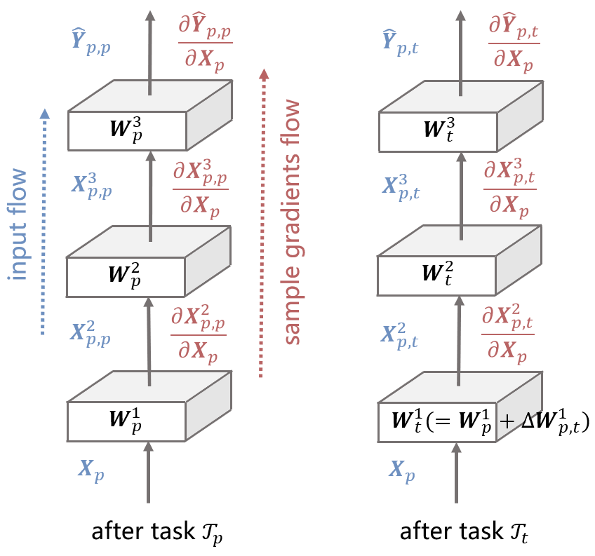
Figure 1: Feeding data $\mathbf{X}_{p}$ into an exemplar neural network after learning task $\mathcal{T}_{p}$ and $\mathcal{T}_{t}\left(p<t\right)$ respectively. $\Delta\mathbf{W}_{p,t}^{l}$ denotes the change of weights in task $\mathcal{T}_{t}$ relative to task $\mathcal{T}_{p}$. If $\Delta\mathbf{W}_{p,t}^{1}$ meets the constraint $\mathbf{X}_{p}\Delta\mathbf{W}_{p,t}^{1}=0$, then $\mathbf{X}_{p,p}^{2}$ is equal to $\mathbf{X}_{p,t}^{2}$. Recursively, the final outputs $\hat{\mathbf{Y}}_{p,t}$ and $\hat{\mathbf{Y}}_{p,p}$ will be identical even the weights of the neural network are updated. More, if $\Delta\mathbf{W}_{p,t}^{l}$ meets another constraint $\frac{\partial\mathbf{X}^{l}_{p,t}}{\partial\mathbf{X}_{p}}\Delta\mathbf{W}_{p,t}^{l}=0$, the sample gradients $\frac{\partial\hat{\mathbf{Y}}_{p,t}}{\partial\mathbf{X}_{p}}$ and $\frac{\partial\hat{\mathbf{Y}}_{p,p}}{\partial\mathbf{X}_{p}}$ will be identical.

In this section, we introduce the preliminary concepts underlying our work.

2.1 Sample Gradient Regularization

The robustness of the neural network trained with IGR has been demonstrated in adversarial examples across multiple attacks, architectures and datasets [3]. IGR optimizes a neural network $f_{\mathbf{w}}$ by minimizing both the classification loss and the rate of change of that loss with respect to samples, formulated as:

$$\mathbf{w}^{\ast}=\underset{\mathbf{w}}{\mathrm{argmin}}H\left(\mathbf{y},\hat{\mathbf{y}}\right)+\lambda\left\|\nabla_{\mathbf{x}}H\left(\mathbf{y},\hat{\mathbf{y}}\right)\right\|,$$ (1)

where $H\left(\cdot,\cdot\right)$ is the cross-entropy and $\lambda$ is a hyper-parameter controlling the regular strength. The second term on the right side is to make the variation of the KL divergence between the final output $\hat{\mathbf{y}}$ and the label $\mathbf{y}$ become as small as possible if any sample $\mathbf{x}$ changes locally.

2.2 Gradient Projection Memory

Consider a sequence of task $\left\{\mathcal{T}_{1},\mathcal{T}_{2},\dots\right\}$ where task $\mathcal{T}_{t}$ is associated with paired dataset $\left\{\mathbf{X}_{t},\mathbf{Y}_{t}\right\}$ of size $n_{t}$. When feeding data $\mathbf{X}_{p}$ from previous task $\mathcal{T}_{p}\left(p<t\right)$ into the neural network with optimal weight $\mathbf{W}_{t}$ for task $\mathcal{T}_{t}$ (see Fig. 1), the input and output of the $l$-th linear block (consisting of a linear layer and an activation function $\eta$) are denoted as $\mathbf{X}_{p,t}^{l}$ and $\mathbf{X}_{p,t}^{l+1}$ respectively, then

$$\mathbf{X}_{p,t}^{l+1}=\mathbf{X}_{p,t}^{l}\mathbf{W}_{t}^{l}\circ\eta=\mathbf{X}_{p,t}^{l}\left(\mathbf{W}_{p}^{l}+\Delta\mathbf{W}_{p,t}^{l}\right)\circ\eta,$$ (2)

where $\Delta\mathbf{W}_{p,t}^{l}$ denotes the change of weights in task $\mathcal{T}_{t}$ relative to task $\mathcal{T}_{p}$. Assuming $\mathbf{X}_{p,t}^{l}=\mathbf{X}_{p,p}^{l}$, a sufficient condition to guarantee $\mathbf{X}_{p,t}^{l+1}=\mathbf{X}_{p,p}^{l+1}$ is by imposing a constraint on $\Delta\mathbf{W}_{p,t}^{l}$ as [5].

$$\mathbf{X}_{p,t}^{l}\Delta\mathbf{W}_{p,t}^{l}=0.$$ (3)

The final output of a fully-connected network with $L$ linear blocks can be expressed as

$$\hat{\mathbf{Y}}_{p,t}=\mathbf{X}_{p}\mathbf{W}_{t}^{1}\circ\eta\circ\mathbf{W}_{t}^{2}\circ\cdots\circ\eta\circ\mathbf{W}_{t}^{L},$$ (4)

where $\mathbf{X}_{p,t}^{1}=\mathbf{X}_{p}$. If Eq. 3 is satisfied on each layer recursively, the final outputs $\hat{\mathbf{Y}}_{p,t}$ and $\hat{\mathbf{Y}}_{p,p}$ of the neural network with distinct weights for task $\mathcal{T}_{t}$ and task $\mathcal{T}_{p}$ are identical. Consequently, the performance on task $\mathcal{T}_{p}$ would be maintained after learning task $\mathcal{T}_{t}$.

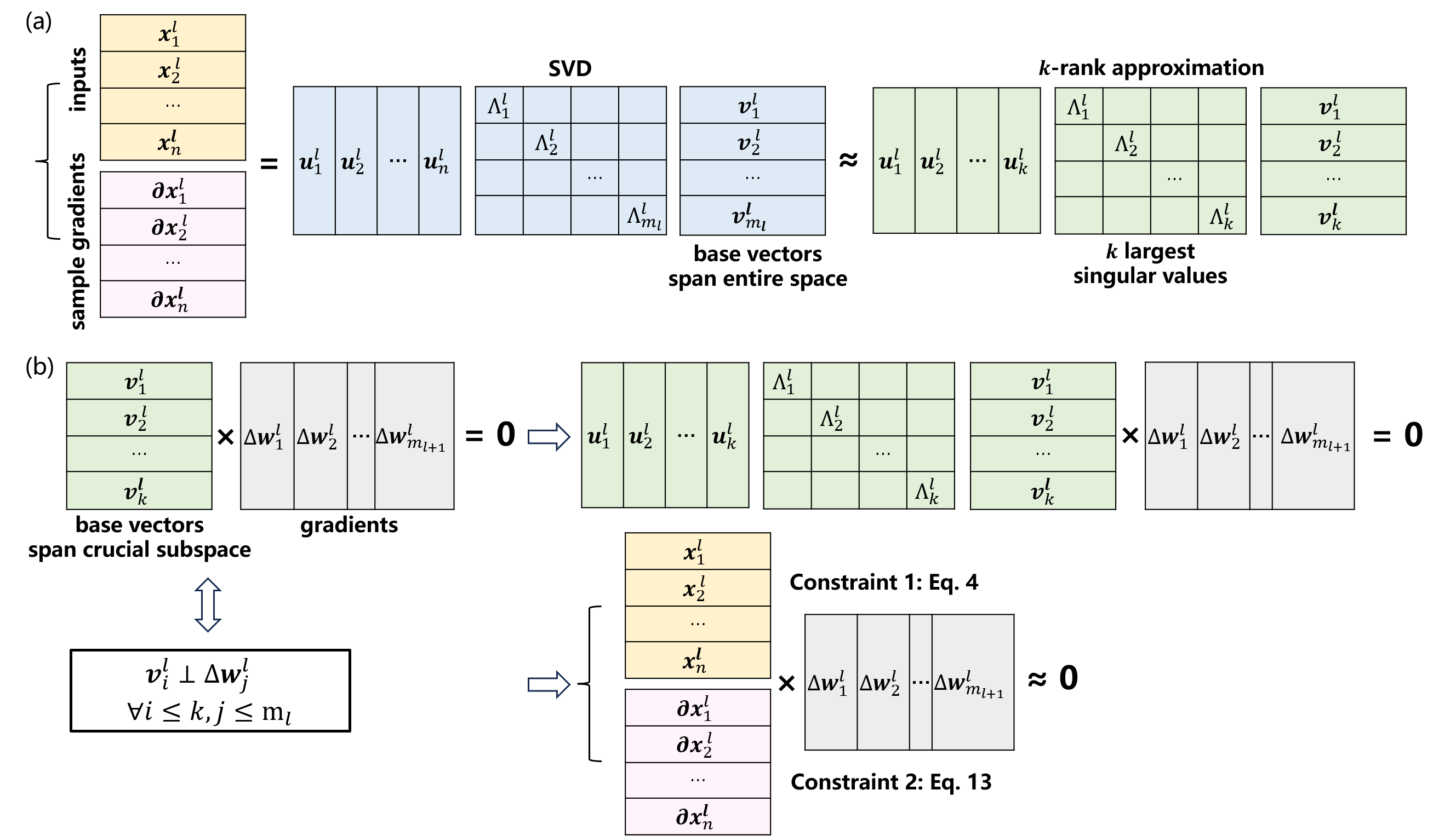
Figure 2: Graphical representation illustrating the imposed constraints in DGP. (a) The $\mathbf{X}^{l}$ or $\frac{d\mathbf{X}^{l}}{d\mathbf{X}}$ is approximated by $\mathbf{U}^{l}_{k}\mathbf{\Lambda}^{l}_{k}\left(\mathbf{V}^{l}_{k}\right)^{\mathrm{T}}$. (b) Multiplication of $\left(\mathbf{V}^{l}_{k}\right)^{\mathrm{T}}$ with $\Delta\mathbf{W}^{l}$ being zero implies that multiplication of $\mathbf{X}^{l}$ (or $\frac{\partial\mathbf{X}^{l}}{\partial\mathbf{X}}$) with $\Delta\mathbf{W}^{l}$ is approximately zero. Consequently, weight updates $\Delta\mathbf{W}^{l}$ have little impact on $\mathbf{X}^{l+1}$ (or $\frac{\partial\mathbf{X}^{l+1}}{\partial\mathbf{X}}$) of previous tasks.

GPM [4] performs singular value decomposition (SVD) on $\mathbf{X}_{p,p}^{l}\in\mathbb{R}^{n\times m_{l}}$, where $n$ is the number of samples randomly drawn from the task $\mathcal{T}_{p}$ and $m_{l}$ is the number of features in an input of $l$-th layer:

$$\mathbf{X}_{p,p}^{l}\Delta\mathbf{W}_{p,t}^{l}=\mathbf{U}^{l}\mathbf{\Lambda}^{l}\left(\mathbf{V}^{l}\right)^{\mathrm{T}}\Delta\mathbf{W}_{p,t}^{l}\approx\mathbf{U}^{l}_{k}\mathbf{\Lambda}^{l}_{k}\left(\mathbf{V}^{l}_{k}\right)^{\mathrm{T}}\Delta\mathbf{W}_{p,t}^{l},$$ (5)

where $\left(\mathbf{V}^{l}\right)^{T}\in\mathbb{R}^{m_{l}\times m_{l}}$ is an orthogonal matrix, of which all the row vectors as a basis span the entire $m_{l}$-dimensional space. Eq. 3 holds true when $\left(\mathbf{V}^{l}\right)^{T}\Delta\mathbf{W}_{p,t}^{l}=0$, indicating that each column vector of $\Delta\mathbf{W}_{p,t}^{l}\in\mathbb{R}^{m_{l}\times m_{l+1}}$ is orthogonal to all the row vectors of $\left(\mathbf{V}^{l}\right)^{T}$. However, it is not possible for a $m_{l}$-dimensional vector to be orthogonal to the entire $m_{l}$-dimensional space unless it is the zero vector, implying no weight update. GPM approximates $\mathbf{X}_{p,p}^{l}$ as $\mathbf{U}^{l}_{k}\mathbf{\Lambda}^{l}_{k}\left(\mathbf{V}^{l}_{k}\right)^{\mathrm{T}}$, where $\left(\mathbf{V}^{l}_{k}\right)^{\mathrm{T}}$ preserves the first $k$ column vectors of $\left(\mathbf{V}^{l}\right)^{\mathrm{T}}$, corresponding to the $k$ largest singular values in diagonal matrix $\mathbf{\Lambda}^{l}$, and spans a subspace of $k\left(<m_{l}\right)$ dimensions. Among all subspaces of $k$ dimensions, weight update orthogonal to this crucial subspace allows for the maximal satisfaction of Eq. 3. An intuitive description is provided in Fig. 2. The value of $k$ is decided by the following criteria:

$$\left\|\mathbf{U}^{l}_{k}\mathbf{\Lambda}^{l}_{k}\left(\mathbf{V}^{l}_{k}\right)^{\mathrm{T}}\right\|_{F}^{2}\geq\alpha^{l}\left\|\mathbf{U}^{l}\mathbf{\Lambda}^{l}\left(\mathbf{V}^{l}\right)^{\mathrm{T}}\right\|_{F}^{2},$$ (6)

where $\alpha^{l}$ is a given threshold representing the trade-off between learning plasticity and memory stability of the model [6]. By establishing a dedicated pool $\mathcal{P}^{l}$ to retain base vectors $\left(\mathbf{V}^{l}_{k}\right)^{\mathrm{T}}$ from previous tasks, GPM enforces the orthogonality of gradients with respect to these base vectors in the learning process of a new task:

$$\nabla_{W^{l}}\mathcal{L}=\nabla_{W^{l}}\mathcal{L}-\left(\nabla_{W^{l}}\mathcal{L}\right)\mathcal{P}^{l}\left(\mathcal{P}^{l}\right)^{T}.$$ (7)

For the convolutional layer, the convolution operator can also be formulated as matrix multiplication. Please refer to [7, 4] for details.

3 Method

In this section, we propose an algorithm drawing inspiration from the IGR and GPM to effectively address the challenge of maintaining adversarial robustness in the continuous learning scenario, where revisiting previous data is not feasible. We hypothesize that adversarial robustness, which has been enhanced by IGR in previous tasks, will hold even after learning a sequence of new tasks, if we can stabilize the smoothed gradients of samples from previous tasks.

3.1 Constraint on Weight Updates

By applying the chain rule for derivatives of composite functions, the gradient of the model’s (with $L$ blocks) final output $\hat{\mathbf{y}}$ with respect to a sample $\mathbf{x}$ can be expressed in terms of recursive multiplication:

$$\frac{\partial\mathbf{x}^{\left(2\right)}}{\partial\mathbf{x}}\frac{\partial\mathbf{x}^{\left(3\right)}}{\partial\mathbf{x}^{\left(2\right)}}\cdots\frac{\partial\hat{\mathbf{y}}}{\partial\mathbf{x}^{L}}=\frac{\partial\hat{\mathbf{y}}}{\partial\mathbf{x}}.$$ (8)

We reformulate Eq. 8 in the Jacobian matrix form

$$\begin{bmatrix}\frac{\partial x_{1}^{\left(2\right)}}{\partial x_{1}}&\cdots&\frac{\partial x_{m_{2}}^{\left(2\right)}}{\partial x_{1}}\\ \vdots&\vdots&\vdots\\ \frac{\partial x_{1}^{\left(2\right)}}{\partial x_{m_{1}}}&\cdots&\frac{\partial x_{m_{2}}^{\left(2\right)}}{\partial x_{m_{1}}}\end{bmatrix}\begin{bmatrix}\frac{\partial x_{1}^{\left(3\right)}}{\partial x_{1}^{\left(2\right)}}&\cdots&\frac{\partial x_{m_{3}}^{\left(3\right)}}{\partial x_{1}^{\left(2\right)}}\\ \vdots&\vdots&\vdots\\ \frac{\partial x_{1}^{\left(3\right)}}{\partial x_{m_{2}}^{\left(2\right)}}&\cdots&\frac{\partial x_{m_{3}}^{\left(3\right)}}{\partial x_{m_{2}}^{\left(2\right)}}\end{bmatrix}\cdots\\ \begin{bmatrix}\frac{\partial\hat{y}_{1}}{\partial x_{1}^{L}}&\cdots&\frac{\partial\hat{y}_{c}}{\partial x_{L}^{l}}\\ \vdots&\vdots&\vdots\\ \frac{\partial\hat{y}_{1}}{\partial x_{m_{L}}^{L}}&\cdots&\frac{\partial\hat{y}_{c}}{\partial x_{m_{L}}^{L}}\end{bmatrix}=\begin{bmatrix}\frac{\partial\hat{y}_{1}}{\partial x_{1}}&\cdots&\frac{\partial\hat{y}_{c}}{\partial x_{1}}\\ \vdots&\vdots&\vdots\\ \frac{\partial\hat{y}_{1}}{\partial x_{m_{1}}}&\cdots&\frac{\partial\hat{y}_{c}}{\partial x_{m_{1}}}\end{bmatrix},$$ (9)

where $m_{l}$ represents the number of features in the input of $l$-th block, and $c$ equals the total number of classes within labels.

3.1.1 Linear block

Stringent guarantee. The gradient of the output $\mathbf{x}^{l+1}$ with respect to the input ${\mathbf{x}^{l}}$ of the $l$-th block is derived as explicitly related to the weights $\mathbf{W}^{l}$:

$$\frac{\partial\mathbf{x}^{l+1}}{\partial\mathbf{x}^{l}}=\mathbf{W}^{l}\left(\eta^{{}^{\prime}}|\mathbf{x}^{l+1}\right)=\begin{bmatrix}w_{1,1}^{l}&\cdots&w_{m_{l+1},1}^{l}\\ \vdots&\vdots&\vdots\\ w_{1,m_{l}}^{l}&\cdots&w_{m_{l+1},m_{l}}^{l}\end{bmatrix}\begin{bmatrix}\eta^{{}^{\prime}}|{x_{1}^{l+1}}&\cdots&0\\ \vdots&\vdots&\vdots\\ 0&\cdots&\eta^{{}^{\prime}}|{x_{m_{l+1}}^{l+1}}\end{bmatrix}.$$ (10)

Each column of the weight matrix (left) represents a single artificial neuron in the linear layer. Element $\eta^{{}^{\prime}}|x_{i}^{l+1}$ in the diagonal matrix (right) represents the derivative of activation function $\eta$ e.g., Relu, of which $\eta^{{}^{\prime}}=1$ if activation $x_{i}^{l+1}>0$, otherwise it is $0$. By combining Eq. 8 and Eq. 10, we can efficiently compute the gradient of each block’s input with respect to the sample based on that of the previous block, i.e., $\frac{\partial\mathbf{x}^{l+1}}{\partial\mathbf{x}}=\frac{\partial\mathbf{x}^{l}}{\partial\mathbf{x}}\frac{\partial\mathbf{x}^{l+1}}{\partial\mathbf{x}^{l}}$, instead of having to compute them from scratch which is time-consuming.

We then impose a constraint on weight updates, akin to Eq. 3 but specifically for stabilizing sample gradients (the core idea of this paper):

$$\frac{\partial\mathbf{X}^{l}_{p,t}}{\partial\mathbf{X}_{p}}\Delta\mathbf{W}_{p,t}^{l}=0.$$ (11)

If Eq. 11 is satisfied on each layer recursively, the sample gradients $\frac{\partial\hat{\mathbf{Y}}_{p,t}}{\partial\mathbf{X}_{p}}$ and $\frac{\partial\hat{\mathbf{Y}}_{p,p}}{\partial\mathbf{X}_{p}}$ of a neural network with distinct weights for task $\mathcal{T}_{t}$ and task $\mathcal{T}_{p}$ are identical (see Fig. 1). Similarly, the method in GPM can be used for an approximate implementation of Eq.11.

Weak guarantee. However, directly performing SVD on the matrix $\frac{\partial\mathbf{X}^{l}}{\partial\mathbf{X}}\in\mathbb{R}^{\left(nm_{1}\right)\times m_{l}}$ is computationally time-consuming due to its large size, which is a concat of multiple $\frac{\partial\mathbf{x}^{l}}{\partial\mathbf{x}}\in\mathbb{R}^{m_{1}\times m_{l}}$. To compress the matrix, we modify $\frac{\partial\mathbf{x}^{\left(2\right)}}{\partial\mathbf{x}}$ through column-wise summation, which is located at the beginning of the matrix chain as depicted in Eq. 8, and substitute it back into Eq. 9 as:

$$\begin{bmatrix}\sum\limits_{i=1}^{m_{1}}\frac{\partial x_{1}^{\left(2\right)}}{\partial x_{i}}&\cdots\sum\limits_{i=1}^{m_{1}}\frac{\partial x_{m_{2}}^{\left(2\right)}}{\partial x_{i}}\end{bmatrix}\begin{bmatrix}\frac{\partial x_{1}^{\left(3\right)}}{\partial x_{1}^{\left(2\right)}}&\cdots&\frac{\partial x_{m_{3}}^{\left(3\right)}}{\partial x_{1}^{\left(2\right)}}\\ \vdots&\vdots&\vdots\\ \frac{\partial x_{1}^{\left(3\right)}}{\partial x_{m_{2}}^{\left(2\right)}}&\cdots&\frac{\partial x_{m_{3}}^{\left(3\right)}}{\partial x_{m_{2}}^{\left(2\right)}}\end{bmatrix}\cdots\\ \begin{bmatrix}\frac{\partial\hat{y}_{1}}{\partial x_{1}^{L}}&\cdots&\frac{\partial\hat{y}_{c}}{\partial x_{L}^{l}}\\ \vdots&\vdots&\vdots\\ \frac{\partial\hat{y}_{1}}{\partial x_{m_{L}}^{L}}&\cdots&\frac{\partial\hat{y}_{c}}{\partial x_{m_{L}}^{L}}\end{bmatrix}=\begin{bmatrix}\sum\limits_{i=1}^{m_{1}}\frac{\partial\hat{y}_{1}}{\partial x_{i}}&\cdots&\sum\limits_{i=1}^{m_{1}}\frac{\partial\hat{y}_{c}}{\partial x_{i}}\end{bmatrix}.$$ (12)

According to Eq. 12, $\frac{\partial\mathbf{x}^{l}}{\partial\mathbf{x}}$ transforms to a vector $\in\mathbb{R}^{m_{l}}$. This modification significantly reduces the computational time required for performing SVD on matrix $\frac{\partial\mathbf{X}^{l}}{\partial\mathbf{X}}\in\mathbb{R}^{n\times m_{l}}$, while relaxes the stringent guarantee for stabilizing $\frac{\partial\hat{\mathbf{y}}}{\partial\mathbf{x}}$ to a less restrictive one (see right-hand side of Eq. 9 and Eq. 12). The target of the constraint in Eq. 11 is altered from stabilizing the gradient of each final output with respect to each feature in the sample, to stabilizing the sum of gradients of each final output with respect to all features in the sample. This weak guarantee is sufficient to yield desirable results in our experiments for both fully-connected and convolutional neural networks.

3.1.2 Convolutional block

The convolutional block consists of a convolution layer, a batch normalization layer (BN) and an activated function. The gradient of the output $\mathbf{x}^{l+1}$ with respect to an input $\mathbf{x}^{l}$ is derived as:

$$\frac{\partial\mathbf{x}^{l+1}}{\partial\mathbf{x}^{l}}=\widetilde{\mathbf{W}}^{l}\partial\mathrm{BN}^{l}\left(\eta^{\prime}\mid\mathbf{x}^{l+1}\right),$$ (13)

where $\partial\mathrm{BN}^{l}$ denotes the gradients in BN. The mean and variance $\sigma^{2}$ per-channel used for normalization are constants during evaluation, if they are calculated by tracking during training [8]. In this case, $\partial\mathrm{BN}^{l}$ is a diagonal matrix with the diagonal element $\frac{\gamma}{\sqrt{\sigma^{2}+\epsilon}}$. Please see Appendix A.4 for the case where the mean and variance are batch statistics.

There are two differences between the convolution layer and the linear layer. First, the $\widetilde{\mathbf{W}}^{l}\in\mathbb{R}^{\left(c_{l}h_{l}\omega_{l}\right)\times\left(c_{l+1}h_{l+1}\omega_{l+1}\right)}$ is distinct from the weight matrix $\mathbf{W}^{l}\in\mathbb{R}^{\left(c_{l}k_{l}k_{l}\right)\times c_{l+1}}$, where each column represents a flattened convolution kernel. Here, $c_{l+1}$ ($k_{l}$) denotes the number (size) of kernels in the $l$-th layer, and $h_{l}$ ($\omega_{l}$) denotes the height (width) of the input $\mathbf{x}^{l}$. We give a simple example to illustrate the composition of $\widetilde{\mathbf{W}}^{l}$ in Appendix Fig. 1. The $\widetilde{\mathbf{W}}^{l}$ is sparse, with non-zero elements only present at specific positions of each column, corresponding to the input features that interact with a convolution kernel. To facilitate implementation, we input $\frac{\partial\mathbf{x}^{l}}{\partial\mathbf{x}}$ into the $l$-th convolution layer after reshaping it from $\left(c_{l}h_{l}\omega_{l},\right)$ into $\left(c_{l},h_{l},\omega_{l}\right)$, and subsequently reshape the output from $\left(c_{l+1},h_{l+1},\omega_{l+1}\right)$ back to $\left(c_{l+1}h_{l+1}\omega_{l+1},\right)$, thereby obviating the intricate construction of $\widetilde{\mathbf{W}}^{l}$.

Second, the base vectors formed by directly performing SVD on $\frac{\partial\mathbf{X}^{l}}{\partial\mathbf{X}}\in\mathbb{R}^{n\times\left(c_{l}h_{l}\omega_{l}\right)}$ can be used to constrain the updates $\Delta\widetilde{\mathbf{W}}^{l}$ rather than $\Delta\mathbf{W}^{l}$. Consequently, we perform SVD after reshaping $\frac{\partial\mathbf{X}^{l}}{\partial\mathbf{X}}$ into a matrix $\in\mathbb{R}^{\left(nh_{l+1}\omega_{l+1}\right)\times\left(c_{l}k_{l}k_{l}\right)}$ (see Appendix Fig. 2 for details).

3.2 Double Gradient Projection (DGP)

The fundamental principle of our algorithm is concise: stabilizing the smoothed sample gradients (some implementation details are elaborated in the preceding subsection). The overall algorithmic flow is outlined as follows: Firstly, the neural network is trained on task $\mathcal{T}_{t}$ using the loss function that includes a penalty term of sample gradients, as shown in Eq. 1. The weight update is projected to be orthogonal to the base vectors in pool $\mathcal{P}$ if the sequential number $t>1$. Subsequently, after training, SVD is performed on the layer-wise inputs $\mathbf{X}^{l}_{t}$ to obtain base vectors that span the first gradient subspaces crucial for stabilizing the final outputs of the neural network on task $\mathcal{T}_{t}$. Lastly, another SVD is performed on the gradients of the layer-wise inputs with respect to the samples $\frac{\partial\mathbf{X}_{t}^{l}}{\partial\mathbf{X}_{t}}$ to obtain base vectors that span the second gradient subspaces crucial for stabilizing the gradients of final outputs with respect to the samples on task $\mathcal{T}_{t}$. Note that in order to eliminate the redundancy between new bases and existing bases in the pool $\mathcal{P}$, both $\mathbf{X}^{l}_{t}$ and $\frac{\partial\mathbf{X}_{t}^{l}}{\partial\mathbf{X}_{t}}$ are projected orthogonally onto $\mathcal{P}^{l}$ prior to performing SVD. Please refer to [4] for details. A compact pseudo-code of our algorithm is presented in Alg. 1.

Algorithm 1 Double Gradient Projection

Input: Training dataset $\left\{\mathbf{X}_{t},\mathbf{Y}_{t}\right\}$ for task $\mathcal{T}_{t}\in\left\{\mathcal{T}_{1},\mathcal{T}_{2},\dots\right\}$, regularization strength $\lambda$, learning rate $\alpha$
Output: Neural network $f_{w}$ with optimal weights
Initialization: Pool $\mathcal{P}\leftarrow\left\{\right\}$

1:  for  task $\mathcal{T}_{t}\in\left\{\mathcal{T}_{1},\mathcal{T}_{2},\dots\right\}$  do

2:     while  not converged  do

3:        Sample a batch from $\left\{\mathbf{X}_{t},\mathbf{Y}_{t}\right\}$

4:        Calculate $\left\{\nabla_{\mathbf{W}^{l}}\mathcal{L}\right\}$ with the loss $\mathcal{L}$ in Eq. 1

5:        if $t>1$ then

6:           $\nabla_{W^{l}}\mathcal{L}=\nabla_{W^{l}}\mathcal{L}-\left(\nabla_{W^{l}}\mathcal{L}\right)\mathcal{P}^{l}\left(\mathcal{P}^{l}\right)^{T}$ $\forall l=1,2,...,L$ $\triangleright$ Gradient projection for each layer

7:        end if

8:        $\mathbf{W}^{l}\leftarrow\mathbf{W}^{l}-\alpha\nabla_{\mathbf{W}^{l}}\mathcal{L}$ $\triangleright$ Weight update

9:     end while

10:     $\mathbf{X}^{l}_{t}\leftarrow\mathbf{X}^{l}_{t}-\mathcal{P}^{l}\left(\mathcal{P}^{l}\right)^{T}\mathbf{X}^{l}_{t}$ $\triangleright$ Ensure uniqueness of new bases

11:     Perform SVD on $\mathbf{X}^{l}_{t}$ and put bases into $\mathcal{P}^{l}$ $\triangleright$ Construct first gradient subspace

12:     $\frac{\partial\mathbf{X}_{t}^{l}}{\partial\mathbf{X}_{t}}\leftarrow\frac{\partial\mathbf{X}^{l}_{t}}{\partial\mathbf{X}_{t}}-\mathcal{P}^{l}\left(\mathcal{P}^{l}\right)^{T}\frac{\partial\mathbf{X}^{l}_{t}}{\partial\mathbf{X}_{t}}$

13:     Perform SVD on $\frac{\partial\mathbf{X}_{t}^{l}}{\partial\mathbf{X}_{t}}$ and put bases into $\mathcal{P}^{l}$ $\triangleright$ Construct second gradient subspace

14:  end for

4 Experiment

4.1 Step

Baselines. For continual learning [9], we adopt (1) SGD, which serves as a naive baseline using stochastic gradient descent to optimize the neural network, (2) EWC [10], (3) SI [11], (4) GEM [12], (5) A-GEM [13], (6) OGD [1] and (7) GPM. For adversarial robustness, we adopt (8) IGR, and (9) Distillation [14].

We combine the methods from fields of continual learning (1$\sim$7) and adversarial robustness (8$\sim$9), such as EWC + IGR, to establish the baselines for continual robust learning. Additionally, we apply the FGSM [15], PGD [16], and AutoAttack [17] to generate adversarial attacks.

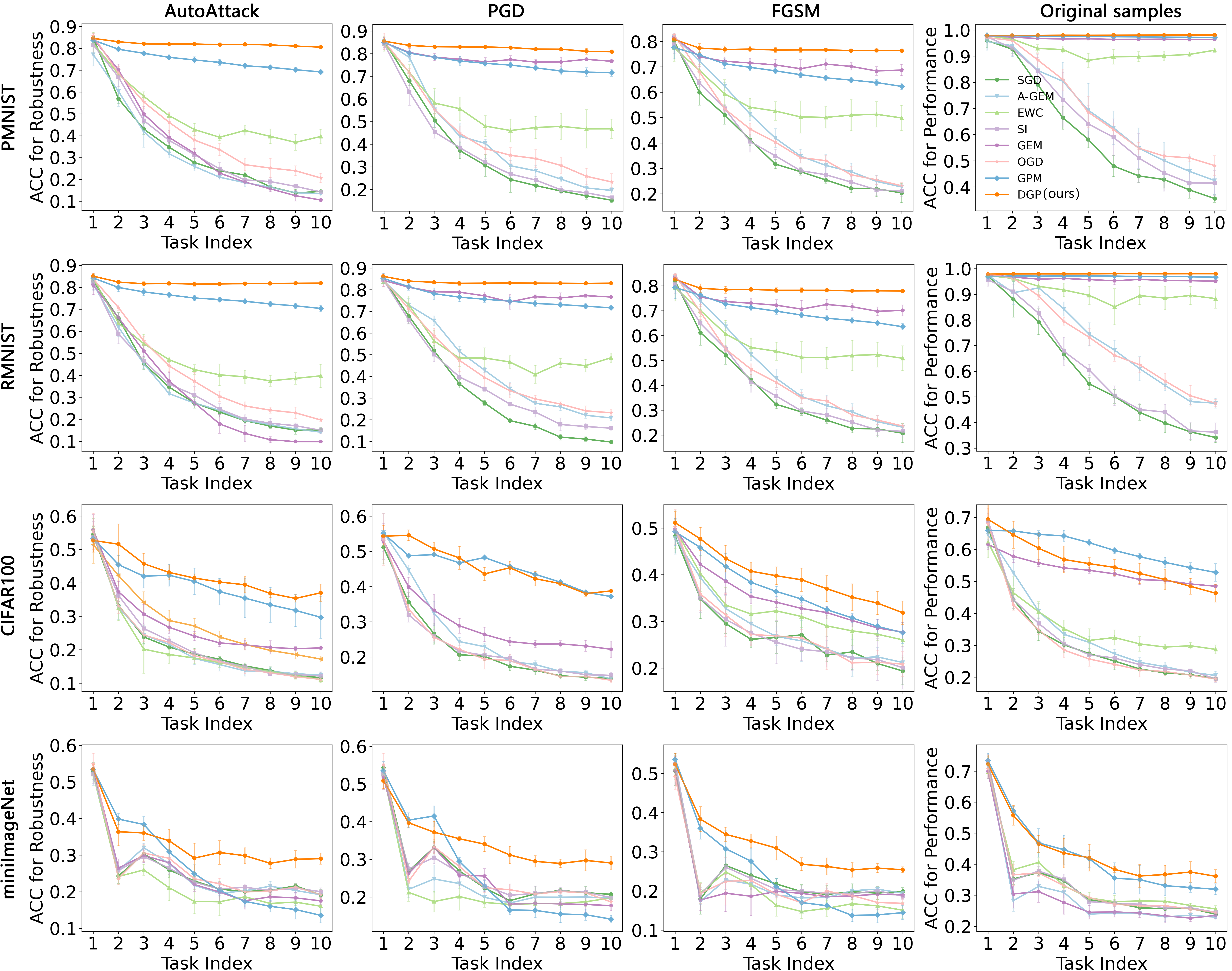
Figure 3: ACC varying with the number of learned tasks on datasets of Permuted MNIST (first row), Rotated MNIST (second row), CIFAR100 (third row) and miniImageNet (fourth row). ACC is measured on adversarial samples generated by AutoAttack (first column), PGD (second column) and FGSM (third column), as well as original samples (fourth column). The horizontal axis indicates the number of tasks learned by the neural network at present. The defense strategy used here is IGR. Errors bars denote standard deviation.

Metrics. We use average accuracy (ACC) and backward transfer (BWT) defined as

$$\mathrm{ACC}=\frac{1}{T}\sum_{t=1}^{T}R_{T,t},\quad\quad\quad\quad\quad\mathrm{BWT}=\frac{1}{T-1}\sum_{t=1}^{T-1}R_{T,t}-R_{t,t},$$ (14)

where $R_{T,t}$ denotes the accuracy of task $t$ at the end of learning task $T$. To evaluate the performance of continuous learning, we measure accuracy on test data from previous tasks. To evaluate the adversarial robustness, we then perturb test data, and re-measure accuracy on the corresponding adversarial samples.

Benchmarks. We evaluate our approach on four supervised benchmarks. Permuted MNIST and Rotated MNIST are variants of MNIST dataset of handwritten digits with 10 tasks applying random permutations of the input pixels and random rotations of the original images respectively [18, 19]. Split-CIFAR100 [11] is a random division of CIFAR100 into 10 tasks, each with 10 different classes. Split miniImageNet is a random division of a subset of the original ImageNet dataset [20] into 10 tasks, each with 5 different classes.

Architectures: The neural network architecture varies across experiments: a fully connected network is used for the MNIST experiments, an AlexNet for the Split-CIFAR100 experiment, and a variant of ResNet18 for the Split-miniImageNet experiment. In both Split-CIFAR100 and Split-miniImageNet experiments, each task has an independent classifier without constraints on weight updates.

The values of $\frac{\partial\mathbf{x}^{2}}{\partial\mathbf{x}}$ (initial term in Eq.10) are solely determined by the weights of the first layer when feeding the same samples (see Fig.1). There are two options to make $\frac{\partial\mathbf{x}^{2}_{p,t}}{\partial\mathbf{x}_{p}}=\frac{\partial\mathbf{x}^{2}_{p,p}}{\partial\mathbf{x}_{p}}$: fixing the first layer after learning task $p$ or assigning an independent first layer to each task. The latter option is chosen for all experiments, as the former seriously diminishes the neural network’s learning ability in subsequent tasks. To ensure fairness, the same setup is applied to the baselines. Further details on architectures can be found in Appendix B.2.

Training details: For the MNIST experiments, the batch size, number of epochs, and input gradient regularization $\lambda$ are set to 32/10/50, respectively. In the Split-CIFAR100 experiments, the values are 10/100/1, and for the Split-miniImageNet experiments, they are 10/20/1. SGD is used as the optimizer. All reported results are averaged over 5 runs with different seeds. The hyperparameter configurations for algorithms of adversarial attack and continuous learning are provided in Appendix B.3.

4.2 Results

4.2.1 Adversarial Robustness

The robustness results on various datasets are presented in left three columns of Fig. 3. Under attacks with different strengths (AutoAttack $>$ PGD $>$ FGSM), the proposed approach (orange lines) consistently exhibits a high level of effectiveness in preserving the robustness of neural networks during continuous learning. In contrast, the baseline such as IGR+GEM (purple lines), which performs well on MNIST datasets against PGD and FGSM attacks, demonstrates a significant decrease when fronted with AutoAttack. The advantage of our approach becomes even more evident when the number of learned tasks increases.

In Fig. 3, the different color lines represent baselines combined by IGR with various methods of continuous learning. Except for the specifically tailored DGP, these methods do not maintain robustness well gained by IGR when the neural network parameters change to learn new tasks. To provide a comprehensive comparison, we include additional experimental results in Fig. 4, focusing on combinations of Distillation with methods of continuous learning. Distillation is another well-known defense method [21] that involves training two models - a teacher model is trained using one-hot ground truth labels and a student model is trained using the softmax probability outputs of the teacher model. The result demonstrates the model’s robustness gained by Distillation is also not effectively maintained against AutoAttack and PGD attacks after learning a sequence of new tasks.

Considering the collective insights presented in Figs. 3 and 4, it is crucial to underscore that the pursuit of an effective defense demands a specially tailored algorithm adept at accommodating variations in model parameters. Mere combinations of existing defense strategies and continual learning methods, as demonstrated in our experiments, fall short of achieving the desired goal of continuous robustness. Our work contributes to the exploration of this under-researched and challenging research direction.

Moreover, there is a notable trend in Fig.4d: the blue line (representing the performance of Distill+GPM on original samples) exhibits a more rapid decline compared to the corresponding blue line in the fourth subplot of the first row in Fig.3 (representing IGR+GPM). Additionally, the purple and blue lines in Fig.4d (representing Distill+GEM and Distill+GPM) closely align with the green line in Fig.4d (representing Distill+SGD). These observations suggest incorporating Distillation into the training procedure compromise the efficacy of these continual learning methods.

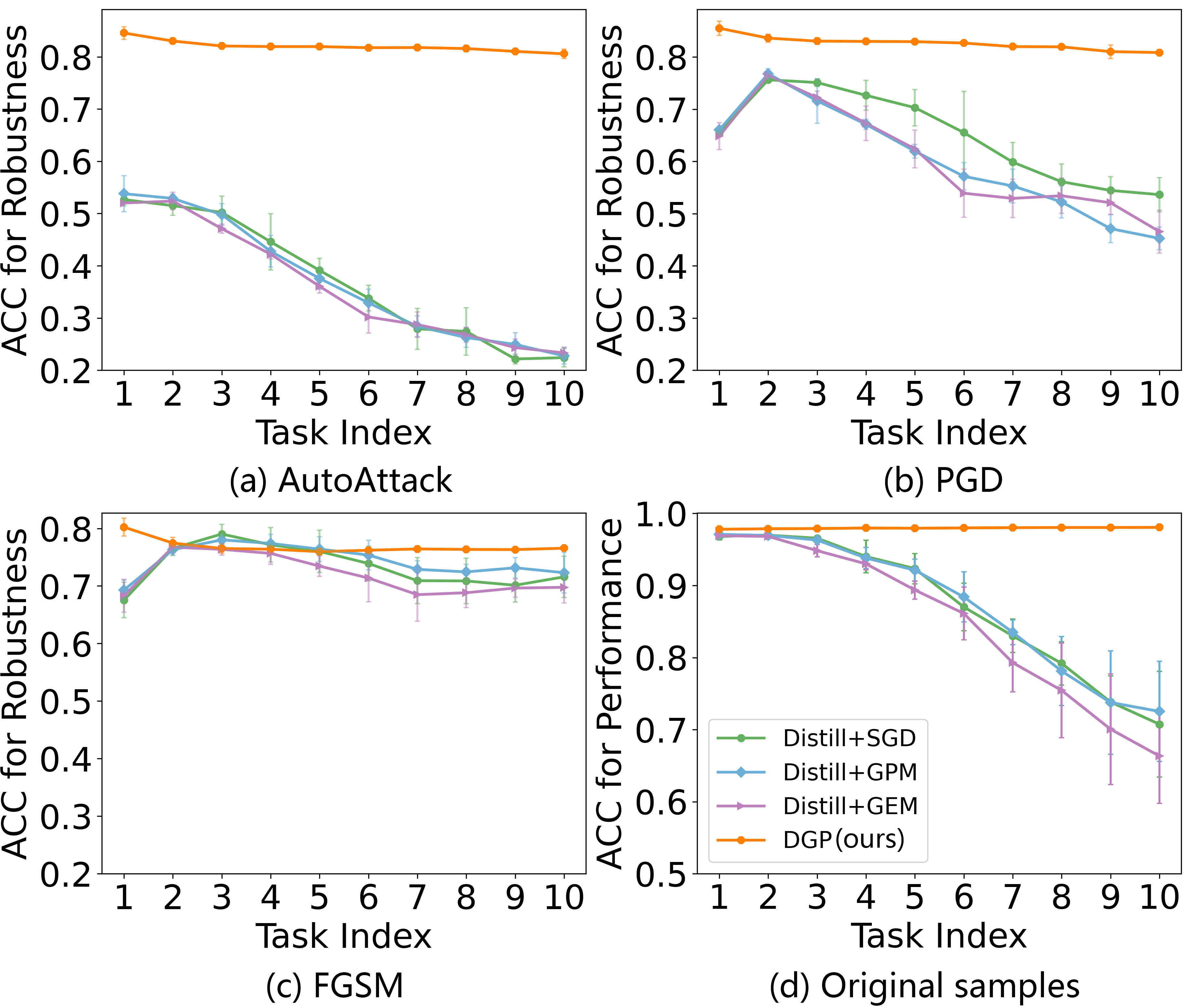
Figure 4: As Fig. 3, but for the defense strategy Distillation on PMNIST dataset. Continual learning methods GEM and GPM are selected to combine with Distillation here, which show superior ACC in Fig. 3 compared to other baselines.

4.2.2 Performance

We also assess the ability of the proposed approach for continual learning (ACC on original samples), as illustrated in the fourth column of Fig. 3. Our DGP algorithm demonstrates comparable performance to GPM and GEM on datasets of Permuted MNIST and Rotated MNIST, effectively addressing the issue of catastrophic forgetting on these two datasets. However, results on the datasets of Split-CIFAR indicate that the performance of DGP is slightly inferior to GDP. We speculate that the reason for this could be that DGP stores a larger number of bases after each task than GPM, as DGP constrains the weight updates to be orthogonal to two crucial subspaces – one for stabilizing the final output (required in GPM) and another for stabilizing the sample gradients. Orthogonality to more base vectors restricts weight updates to a narrower subspace, thereby limiting the plasticity of the model. Overall, our approach effectively maintains adversarial robustness while exhibiting continual learning ability.

In addition, it is noteworthy that the performance curves of several classical continual learning methods closely approximate that of naive SGD (green lines). This observation suggest again potential incompatibility between defense strategies (here IGR, i.e., sample gradient penalty) and continuous learning methods. Additional experimental results are provided in Appendix B.1.

4.2.3 Stabilization of sample gradients

Our approach maintains adversarial robustness by stabilizing the smoothed sample gradients. To valid its stabilization effect, we record the variation of sample gradients on the first task during continuous learning process. Specifically, we randomly select $n$ samples at the end of learning $\mathcal{T}_{1}$ and compute their gradients related to correspondingly final outputs. After learning each new task $\mathcal{T}_{t}$, we recompute their gradients. The variation of gradients between $\mathcal{T}_{1}$ and $\mathcal{T}_{t}$ is quantified by similarity measure:

$$\mathrm{Sim}=\frac{\mathbf{g}_{1}\mathbf{g}_{t}}{\left|\mathbf{g}_{1}\right|\left|\mathbf{g}_{t}\right|},$$ (15)

where $\mathbf{g}$ is a flattened vector of sample gradients. The results on various datasets are presented in Fig. 5. The orange line (representing DGP) shows a relatively flat downward trend, demonstrating the proposed approach indeed has the effect of stabilizing the sample gradients of previous tasks, even after weights of the neural network have been updated.

5 Related Work

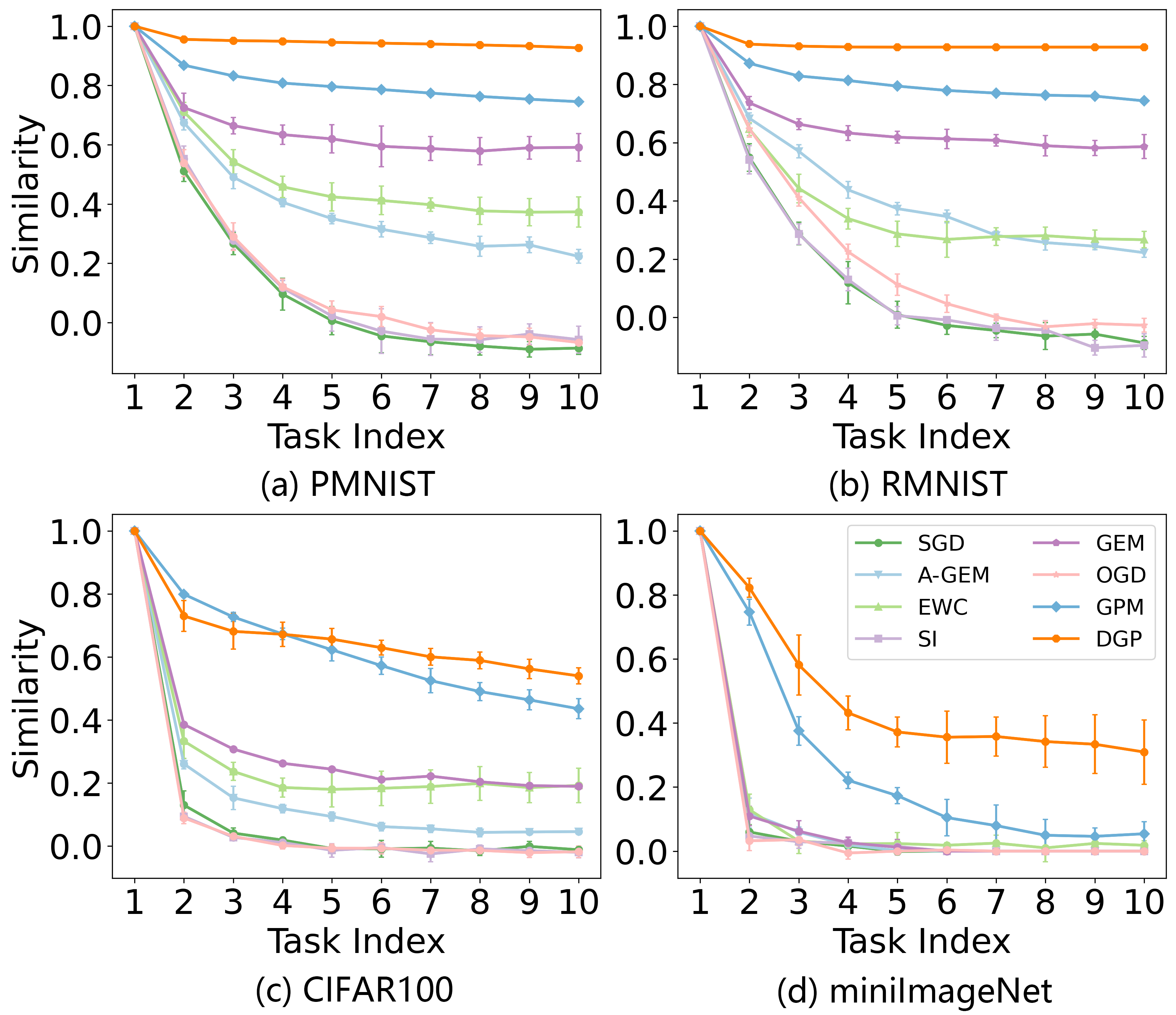
Figure 5: Gradient variation of samples from the first task $\mathcal{T}_{1}$ during continuous learning process. The variations are quantified through similarity.

Continual Learning: Optimization. This class of continual learning approaches design and manipulate the optimization programs explicitly, often employing gradient projection as a typical strategy [22]. Replay-based methods like GEM [12] and A-GEM [13] impose constraints on weight updates to align with the direction of experience replay, thereby preserving previous input space and gradient space through historical training samples. Without saving historical training samples, OWM [23] and AOP [24] modify weight updates to the orthogonal direction of the input space of previous tasks. OGD [1] stores the gradient directions of previous tasks and orthogonalizes the current gradient (the gradients of all parameters are combined into a single vector) with respect to them. FS-DGPM [25] dynamically releases unimportant bases of GPM to improve learning plasticity and encourages the convergence towards a flat loss landscape. In contrast to OGD and GPM, Adam-NSCL [5] directly projects candidate weight updates into the unimportant gradient subspace, i.e., the current null space of the uncentered feature covariance from the previous tasks.

Adversarial Robustness: Regularization. As several attack algorithms rely on the model’s gradient to estimate local optima perturbations that can deceive the classifier, a stream of research has focused on adversarial robust optimization by applying regularization approaches to mitigate the impact of small input perturbations on output decisions, such as the spectral norm of the model’s Jacobian matrix [26], the spectral norm of the weight matrix [27] and the generated adversarial perturbation [28].

Our research does not focus on innovation in the single field of continual learning or adversarial robustness, but rather explores a novel direction that requires their integration. It expands the investigation of adversarial robustness to continuous learning scenarios, which holds significant value for enhancing the security and credibility of artificial intelligence systems in their adaptive evolution across multiple tasks or data domains.

6 Limitation and Discussion

In this work, we observe that the adversarial robustness gained by sophisticated defense strategies is easily erased when the neural network learns new knowledge. The direct combinations of existing defense strategies and continuous learning methods fail to effectively address this issue. In the context of continuous learning, a tailored algorithm is necessary to maintain the robustness brought originally by defense strategies. Therefore, we propose Double Gradient Projection, an approach that can prevents the adversarial robustness from rapidly degradation in the face of changes in model parameters.

From the experimental results, our approach has a limitation: as the number of base vectors becomes large, the stability of the neural network is enhanced to hold both robustness and performance across previous tasks. However, the plasticity of the neural network is restricted, which potentially reduces its learning ability for new tasks. Besides, the memory and computational time of our approach are double that of GPM, due to performing SVD twice after each learned task. If there are numerous tasks and the matrix consisting of orthogonal bases reaches full rank, we could approximate this matrix by performing SVD and selecting column vectors corresponding to a fraction of the largest singular values as the new orthogonal bases to free up the rank space.

Appendix A Method

A.1 Sample Gradients

The sample gradients we stabilize in Sec. Method refer to the gradients of the final outputs with respect to samples, rather than gradients of the loss with respect to samples, which are penalized in IGR. Here, we show their relationship:

$$\frac{\partial\mathbf{\mathcal{L}}}{\partial\mathbf{x}}=\frac{\partial\mathbf{\mathcal{L}}}{\partial\hat{\mathbf{y}}}\frac{\partial\hat{\mathbf{y}}}{\partial\mathbf{x}}=g\left(\hat{\mathbf{y}}\right)\frac{\partial\hat{\mathbf{y}}}{\partial\mathbf{x}},$$ (16)

Where $g$ is a function of $\hat{\mathbf{y}}$. The stabilization of both final outputs $\hat{y}$ and sample gradients $\frac{\partial\hat{\mathbf{y}}}{\partial\mathbf{x}}$ together can result in the stabilization of $\frac{\partial\mathbf{\mathcal{L}}}{\partial\mathbf{x}}$. To maintain the adversarial robustness, achieved by reducing the sensitive of predictions (i.e., final outputs) to subtle changes in samples, it is sufficient to stabilize the smoothed $\frac{\partial\hat{\mathbf{y}}}{\partial\mathbf{x}}$.

A.2 Matrix Composition

A simple example to illustrate the composition of $\widetilde{\mathbf{W}}^{l}$ is depicted in Fig. 6.

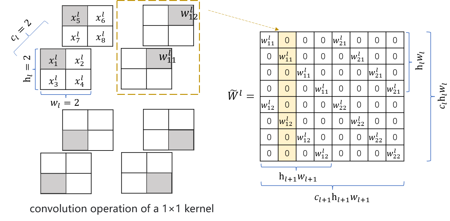
Figure 6: Graphic illustration of an example $\widetilde{\mathbf{W}}^{l}$. The shape of an example input $\mathbf{x}^{l}$ and a convolutional kernel $\mathbf{w}^{l}_{i}$ of $l$-th layer is $\left(2,2,2\right)$ and $\left(2,1,1\right)$ respectively. Suppose there are two convolution kernels in total, i.e., $c_{l+1}=2$. The length of each column vector in $\widetilde{\mathbf{W}}^{l}$ is same as the flattened $\mathbf{x}^{l}$, i.e., $c_{l}h_{l}\omega_{l}=2\times 2\times 2=8$. The four subplots in left display the convolution operation of the kernel $\mathbf{w}^{l}_{1}$ on $\mathbf{x}^{l}$, with grey checks indicating the specific input features on which the kernel acts after each slide. The four subplots sequentially correspond to the first four columns of the example $\widetilde{\mathbf{W}}^{l}$. The non-zero elements within each column of $\widetilde{\mathbf{W}}^{l}$ only present (filled by weights of a kernel) at positions corresponding to those specific input features, while the remains are zero-filled.

A.3 Reshape Prior to Performing SVD

A simple example to illustrate why and how to reshape $\frac{\partial\mathbf{X}^{l}}{\partial\mathbf{X}}$ is depicted in Fig. 7.

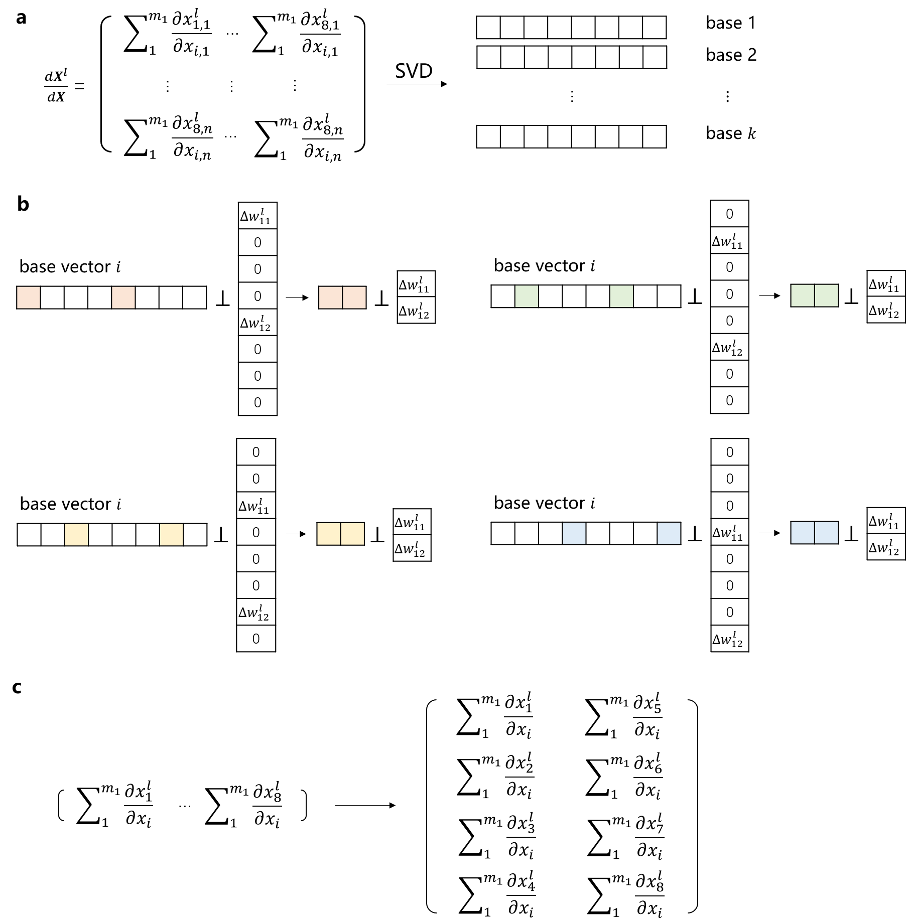
Figure 7: (a) Performing SVD on an example $\frac{\partial\mathbf{X}^{l}}{\partial\mathbf{X}}$ with the shape $(n,c_{l}h_{l}w_{l})$ obtains the base vectors that can constrain the updates $\Delta\widetilde{\mathbf{W}}^{l}$. Here, $x_{i,j}^{l}$ denotes the $i$-th feature of $j$-th input of $l$-th layer, and an single input $\mathbf{x}^{l}$ from $\mathbf{X}^{l}$ is illustrated on the left of Fig. 6. (b) The orthogonality between any base vector and each $h_{l+1}w_{l+1}(=4)$ column vectors of $\widetilde{\mathbf{W}}^{l}$ (see the right of Fig.6) is equivalent to the orthogonality between $h_{l+1}w_{l+1}$ sub-vectors of the base vector and the weight $\mathbf{w}^{l}$ of the kernel. (c) Prior to performing SVD, each row vector in $\frac{\partial\mathbf{X}^{l}}{\partial\mathbf{X}}$ is reshaped into a matrix consisting of $h_{l+1}w_{l+1}$ row vectors with a length of $c_{l}k_{l}k_{l}$. Consequently, the shape of $\frac{\partial\mathbf{X}^{l}}{\partial\mathbf{X}}$ is modified to $(nh_{l+1}w_{l+1},c_{l}k_{l}k_{l})$.

A.4 Gradients in Batch Normalization Layer

The batch normalization (BN) operation is formalized as

$$x_{i}^{out}=\frac{x_{i}^{in}-\mu}{\sqrt{\sigma^{2}+\epsilon}}*\gamma+\beta,$$ (17)

Where $\gamma$ and $\beta$ is the learnable weights. When the mean $\mu$ and variance $\sigma^{2}$ per-channel are batch statistics, $x_{i}^{out}$ (feature $i$ in the output of BN) is not only correlated with $x_{i}^{in}$ (feature $i$ in the input of BN), but with the other features of the same channel in the whole batch samples. Therefore, the Jacobian matrix of the $l$-th BN (after $l$-th convolution layer, as shown in Eq. 14 of main text) is a matrix across batch samples with the shape $\left(nc_{l+1}h_{l+1}\omega_{l+1},nc_{l+1}h_{l+1}\omega_{l+1}\right)$, where each element $\frac{\partial x_{i}^{out}}{\partial x_{j}^{in}}$ is given by:

$$\begin{cases}\gamma\left[-\left(1-\frac{1}{n}\right)\frac{1}{\sqrt{\sigma^{2}+\epsilon}}-\frac{1}{\left(n-1\right)(\sigma^{2}+\epsilon)^{\frac{3}{2}}}\left(x_{i}-\mu\right)^{2}\right]&\text{ if }i=j,\\ \\ \gamma\left[-\frac{1}{n\sqrt{\sigma^{2}+\epsilon}}-\frac{1}{\left(n-1\right)(\sigma^{2}+\epsilon)^{\frac{3}{2}}}\left(x_{i}-\mu\right)\left(x_{j}-\mu\right)\right]&\text{ if }i\neq j\text{ and }x_{i},x_{j}\text{ are in same channel},\\ \\ 0&\text{ others}.\end{cases}$$ (18)

However, due to its extensive scale, the storage or computation of this Jacobian matrix poses high hardware requirements. To facilitate implementation, we propose decomposing this Jacobian matrix into $c_{l+1}$ submatrices with the shape $\left(nh_{l+1}w_{l+1},nh_{l+1}w_{l+1}\right)$, of which all elements belong to the same channel. Subsequently, these submatrices are concatenated to form a new matrix with shape $\left(c_{l+1},nh_{l+1}w_{l+1},nh_{l+1}w_{l+1}\right)$, which effectively optimizes memory usage by eliminating a significant number of zero elements compared to the original Jacobian matrix. Before multiplying with this new matrix, the input gradient matrix of BN should be reshaped from $\left(n,c_{l+1}h_{l+1}w_{l+1}\right)$ to $\left(c_{l+1},nh_{l+1}w_{l+1}\right)$.

Appendix B Experiment

B.1 ACC and BWT on various datasets

The comparisons of ACC and BWT, after learning all the tasks, are presented in Tab. 1 for Permuted MNIST, Tab. 2 for Rotated MNIST and Tab. 3 for Split-CIFAR100 datasets. The majority of baselines exhibit low accuracy (approaching random classification) quickly on the Split-miniImageNet dataset. Therefore, we do not compute BTW for Split-miniImageNet dataset.

Method	Permuted MNIST
	AutoAttack		PGD		FGSM		Original samples
	ACC(%)	BWT	ACC(%)	BWT	ACC(%)	BWT	ACC(%)	BWT
SGD	14.1	-0.75	15.4	-0.74	21.8	-0.67	36.8	-0.66
SI	14.3	-0.76	16.5	-0.76	22.3	-0.68	36.9	-0.67
A-GEM	14.1	-0.69	19.7	-0.66	22.9	-0.67	48.4	-0.54
EWC	39.4	-0.47	43.1	-0.48	50.0	-0.35	84.9	-0.12
GEM	12.1	-0.73	75.5	-0.09	72.8	-0.09	96.4	-0.01
OGD	19.7	-0.72	24.1	-0.67	26.0	-0.63	46.8	-0.57
GPM	70.4	-0.11	72.9	-0.10	65.7	-0.12	97.2	-0.01
DGP	81.6	-0.01	81.2	-0.01	75.8	-0.03	97.6	-0.01

Table 1: Comparisons of ACC and BWT after learning all the tasks on the Permuted MNIST dataset.

Method	Rotated MNIST
	AutoAttack		PGD		FGSM		Original samples
	ACC(%)	BWT	ACC(%)	BWT	ACC(%)	BWT	ACC(%)	BWT
SGD	14.1	-0.76	9.9	-0.76	20.4	-0.69	32.3	-0.71
SI	13.9	-0.77	15.3	-0.73	20.1	-0.70	33.0	-0.72
A-GEM	14.1	-0.69	21.6	-0.69	24.8	-0.63	45.4	-0.57
EWC	45.1	-0.42	49.5	-0.36	46.5	-0.25	80.7	-0.18
GEM	11.9	-0.73	76.5	-0.08	74.4	-0.08	96.7	-0.01
OGD	19.7	-0.72	23.8	-0.68	23.8	-0.64	48.0	-0.55
GPM	68.8	-0.1	71.5	-0.11	65.9	-0.12	97.1	-0.01
DGP	81.6	0.02	82.6	0.01	78.6	-0.01	98.1	-0.00

Table 2: Comparisons of ACC and BWT after learning all the tasks on the Rotated MNIST dataset.

Method	Split-CIFAR100
	AutoAttack		PGD		FGSM		Original samples
	ACC(%)	BWT	ACC(%)	BWT	ACC(%)	BWT	ACC(%)	BWT
SGD	10.3	-0.45	12.8	-0.45	46.5	-0.25	19.4	-0.49
SI	13.0	-0.45	15.2	-0.43	45.4	-0.28	19.8	-0.48
A-GEM	12.6	-0.46	12.9	-0.43	40.6	-0.33	20.7	-0.48
EWC	12.6	-0.43	23.2	-0.31	56.8	-0.15	30.5	-0.35
GEM	21.2	-0.33	19.4	-0.36	60.6	-0.11	47.7	-0.13
OGD	11.8	-0.45	14.1	-0.44	44.2	-0.29	18.9	-0.50
GPM	34.4	-0.13	36.6	-0.17	58.2	-0.16	53.7	-0.10
DGP	36.6	-0.12	39.2	-0.09	67.2	-0.06	48.0	-0.13

Table 3: Comparisons of ACC and BWT after learning all the tasks on the Split-CIFAR100 dataset.

B.2 Architecture Details of Neural Networks

MLP: The fully-connected network in Permuted MNIST and Rotated MNIST experiments consists of three linear layers with 256/256/10 hidden units. No bias units are used. The activation function is Relu. Each task has an independent first layer without constraints imposed on its weight update.

AlexNet: The modified Alexnet[29] in the Split-CIFAR100 experiment consists of three convolutional layers with 32/64/128 kernels of size $\left(4\times 4\right)$/$\left(3\times 3\right)$/$\left(2\times 2\right)$, and three fully connected layers with 2048/2048/10 hidden units. No bias units are used. Each convolution layer is followed by a $\left(2\times 2\right)$ average-pooling layer. The dropout rate is 0.2 for the first two convolutional layers and 0.5 for the remaining layers. The activation function is Relu. Each task has an independent first layer and final layer (classifier) without constraints imposed on its weight update.

ResNet18: The variant ResNet18[30] in the Split-miniImageNet experiment consists of 17 convolutional blocks and one linear layer. The convolutional block comprises a convolutional layer and a batch normalization layer and an Relu activation. The first and last convolutional blocks are followed by a $\left(2\times 2\right)$ average-pooling layer respectively. All convolutional layers use $\left(1\times 1\right)$ zero-padding and kernels of size $\left(3\times 3\right)$. The first convolutional layer has 40 kernels and $\left(2\times 2\right)$ stride, followed by four basic modules, each comprising four convolutional blocks with same number of kernels 40/80/160/320 respectively. The first convolutional layer in each basic modules has $\left(2\times 2\right)$ stride, while the remaining three convolutional layers have $\left(1\times 1\right)$ stride. The skip-connections occur only between basic modules. No bias units are used. In batch normalization layers, tracking mean and variance is used, and the affine parameters are learned in the first task $\mathcal{T}_{1}$, which are then fixed in subsequent tasks. Each task has an independent first layer and final layer.

B.3 Hyper-parameter Configurations

Adversarial attack method method.

dataset	Attack method
	AutoAttack	PGD	FGSM
PMNIST	$\epsilon=20/255$	$\xi=2/255$,$\delta=40/255$	$\xi=25/255$
RMNIST	$\epsilon=20/255$	$\xi=2/255$,$\delta=40/255$	$\xi=25/255$
Split-CIFAR100	$\epsilon=2/255$	$\xi=1/255$,$\delta=4/255$	$\xi=4/255$
Split-miniImageNet	$\epsilon=2/255$	$\xi=1/255$,$\delta=4/255$	$\xi=2/255$

Table 4: Hyper-parameter setup for different adversarial attacks

Continuous learning method. We run the methods of SI, EWC, GEM, A-GEM based on the Avalanche [9], an end-to-end continual learning library. In DGP, $\alpha_{1}$ and $\alpha_{2}$ (see $\alpha$ in Eq. 7 of main text) control the number of base vectors added into the pool for stabilizing the final output and sample gradients respectively. $\alpha_{3}$ is used in reducing the number of base vectors when the pool is full (by performing the SVD and $k$-rank approximation on the matrix consisting of all base vectors in the pool).

Dataset	Method	Hyperparameter
		Learning rate	Others
Permuted MNIST	SGD	0.1	None
	SI	0.1	$\lambda=0.1$
	EWC	0.1	$\lambda=10$
	GEM	0.05	patterns_per_exp $=200$
	A-GEM	0.1	sample_size $=64$, patterns_per_exp $=200$
	OGD	0.05	memory_size $=300$
	GPM	0.05	memory_size $=300$, $\alpha 1=\left[0.95,0.99,0.99\right]$
	DGP	0.05	memory_size $=300$, $\alpha 1=[0.95,0.99,0.99]$, $\alpha 2=0.999$, $\alpha 3=0.996$
Rotated MNIST	SGD	0.1	None
	SI	0.1	$\lambda=0.1$
	EWC	0.1	$\lambda=10$
	GEM	0.05	patterns_per_exp $=200$
	A-GEM	0.1	sample_size $=64$, patterns_per_exp $=200$
	OGD	0.05	memory_size $=300$
	GPM	0.05	memory_size $=300$, $\alpha 1=[0.95,0.99,0.99]$
	DGP	0.05	memory_size $=300$, $\alpha 1=[0.95,0.99,0.99]$, $\alpha 2=0.999$, $\alpha 3=0.996$
Split- CIFAR100	SGD	0.05	None
	SI		$\lambda=0.1$
	EWC		$\lambda=10$
	GEM		patterns_per_exp $=200$
	A-GEM		sample_size $=64$, patterns_per_exp $=200$
	OGD		memory_size $=300$
	GPM		memory_size $=100$, $\alpha 1=0.97+0.003*$task_id
	DGP		memory_size $=100$, $\alpha 1=0.97+0.003*$task_id, $\alpha 2=0.996$, $\alpha 3=0.99$
Split- miniImageNet	SGD	0.1	None
	SI		$\lambda=0.1$
	EWC		$\lambda=10$
	GEM		patterns_per_exp $=200$
	A-GEM		sample_size $=64$, patterns_per_exp $=200$
	OGD		memory_size $=100$
	GPM		memory_size $=100$, $\alpha 1=0.985+0.003*$task_id
	DGP		memory_size $=100$, $\alpha 1=0.96$, $\alpha 2=0.996$, $\alpha 3=0.996$

Table 5: Hyper-parameter setup in our approach and baselines.

References

- [1] Mehrdad Farajtabar, Navid Azizan, Alex Mott, and Ang Li. Orthogonal gradient descent for continual learning. In International Conference on Artificial Intelligence and Statistics, pages 3762–3773. PMLR, 2020.
- [2] Samuel Henrique Silva and Peyman Najafirad. Opportunities and challenges in deep learning adversarial robustness: A survey. arXiv preprint arXiv:2007.00753, 2020.
- [3] Andrew Ross and Finale Doshi-Velez. Improving the adversarial robustness and interpretability of deep neural networks by regularizing their input gradients. In Proceedings of the AAAI conference on artificial intelligence, volume 32, 2018.
- [4] Gobinda Saha, Isha Garg, and Kaushik Roy. Gradient projection memory for continual learning. In International Conference on Learning Representations, 2021.
- [5] Shipeng Wang, Xiaorong Li, Jian Sun, and Zongben Xu. Training networks in null space of feature covariance for continual learning. In Proceedings of the IEEE/CVF conference on Computer Vision and Pattern Recognition, pages 184–193, 2021.
- [6] Liyuan Wang, Xingxing Zhang, Hang Su, and Jun Zhu. A comprehensive survey of continual learning: Theory, method and application. arXiv preprint arXiv:2302.00487, 2023.
- [7] Zhenhua Liu, Jizheng Xu, Xiulian Peng, and Ruiqin Xiong. Frequency-domain dynamic pruning for convolutional neural networks. Advances in neural information processing systems, 31, 2018.
- [8] Sergey Ioffe and Christian Szegedy. Batch normalization: Accelerating deep network training by reducing internal covariate shift. In International conference on machine learning, pages 448–456. pmlr, 2015.
- [9] Vincenzo Lomonaco, Lorenzo Pellegrini, Andrea Cossu, Antonio Carta, Gabriele Graffieti, Tyler L Hayes, Matthias De Lange, Marc Masana, Jary Pomponi, Gido M Van de Ven, et al. Avalanche: an end-to-end library for continual learning. In Proceedings of the IEEE/CVF Conference on Computer Vision and Pattern Recognition, pages 3600–3610, 2021.
- [10] James Kirkpatrick, Razvan Pascanu, Neil Rabinowitz, Joel Veness, Guillaume Desjardins, Andrei A Rusu, Kieran Milan, John Quan, Tiago Ramalho, Agnieszka Grabska-Barwinska, et al. Overcoming catastrophic forgetting in neural networks. Proceedings of the National Academy of Sciences, 114(13):3521–3526, 2017.
- [11] Friedemann Zenke, Ben Poole, and Surya Ganguli. Continual learning through synaptic intelligence. In International conference on machine learning, pages 3987–3995. PMLR, 2017.
- [12] David Lopez-Paz and Marc’Aurelio Ranzato. Gradient episodic memory for continual learning. Advances in neural information processing systems, 30, 2017.
- [13] Arslan Chaudhry, Marc’Aurelio Ranzato, Marcus Rohrbach, and Mohamed Elhoseiny. Efficient lifelong learning with a-gem. In International Conference on Learning Representations, 2019.
- [14] Nicolas Papernot, Patrick Mcdaniel, Xi Wu, Somesh Jha, and Ananthram Swami. Distillation as a defense to adversarial perturbations against deep neural networks. In 2016 IEEE Symposium on Security and Privacy (SP), 2016.
- [15] Alexey Kurakin, Ian J Goodfellow, and Samy Bengio. Adversarial examples in the physical world. In Artificial intelligence safety and security, pages 99–112. Chapman and Hall/CRC, 2018.
- [16] Aleksander Madry, Aleksandar Makelov, Ludwig Schmidt, Dimitris Tsipras, and Adrian Vladu. Towards deep learning models resistant to adversarial attacks. International Conference on Learning Representations, 2018.
- [17] Francesco Croce and Matthias Hein. Reliable evaluation of adversarial robustness with an ensemble of diverse parameter-free attacks. In International conference on machine learning, pages 2206–2216. PMLR, 2020.
- [18] Ian J. Goodfellow, Mehdi Mirza, Da Xiao, Aaron Courville, and Yoshua Bengio. An empirical investigation of catastrophic forgetting in gradient-based neural networks. Computer Science, 84(12):1387–91, 2014.
- [19] Hao Liu and Huaping Liu. Continual learning with recursive gradient optimization. International Conference on Learning Representations, 2022.
- [20] Arslan Chaudhry, Naeemullah Khan, Puneet K. Dokania, and Philip H. S. Torr. Continual learning in low-rank orthogonal subspaces. Advances in Neural Information Processing Systems, 33:9900–9911, 2020.
- [21] Nicholas Carlini and David Wagner. Towards evaluating the robustness of neural networks. In 2017 ieee symposium on security and privacy (sp), pages 39–57. Ieee, 2017.
- [22] Yu Feng and Yuhai Tu. The inverse variance–flatness relation in stochastic gradient descent is critical for finding flat minima. Proceedings of the National Academy of Sciences, 118(9):e2015617118, 2021.
- [23] Guanxiong Zeng, Yang Chen, Bo Cui, and Shan Yu. Continual learning of context-dependent processing in neural networks. Nature Machine Intelligence, 1(8):364–372, 2019.
- [24] Yiduo Guo, Wenpeng Hu, Dongyan Zhao, and Bing Liu. Adaptive orthogonal projection for batch and online continual learning. In Proceedings of the AAAI Conference on Artificial Intelligence, volume 36, pages 6783–6791, 2022.
- [25] Danruo Deng, Guangyong Chen, Jianye Hao, Qiong Wang, and Pheng-Ann Heng. Flattening sharpness for dynamic gradient projection memory benefits continual learning. Advances in Neural Information Processing Systems, 34:18710–18721, 2021.
- [26] Rodrigues, Miguel, R., D., Sokolic, Jure, Giryes, Raja, Sapiro, and Guillermo. Robust large margin deep neural networks. IEEE Transactions on Signal Processing A Publication of the IEEE Signal Processing Society, 2017.
- [27] Cisse Moustapha, Bojanowski Piotr, Grave Edouard, Dauphin Yann, and Usunier Nicolas. Parseval networks: Improving robustness to adversarial examples. pages 854–863, 2017.
- [28] Ziang Yan, Yiwen Guo, and Changshui Zhang. Deepdefense: Training deep neural networks with improved robustness. Advances in Neural Information Processing Systems, 31, 2018.
- [29] Alex Krizhevsky, Ilya Sutskever, and Geoffrey E Hinton. Imagenet classification with deep convolutional neural networks. Advances in neural information processing systems, 25, 2012.
- [30] Arslan Chaudhry, Marcus Rohrbach, Mohamed Elhoseiny, Thalaiyasingam Ajanthan, P Dokania, P Torr, and M Ranzato. Continual learning with tiny episodic memories. In Workshop on Multi-Task and Lifelong Reinforcement Learning, 2019.