AGN properties of $\sim$1 million member galaxies of galaxy groups and clusters at $z<1.4$ based on the Subaru Hyper Suprime-Cam survey

Abstract

Herein, we present the statistical properties of active galactic nuclei (AGNs) for approximately 1 million member galaxies of galaxy groups and clusters, with 0.1 $<$ cluster redshift ($z_{\rm cl}$) $<$ 1.4, selected using Subaru Hyper Suprime-Cam, the so-called CAMIRA clusters. In this research, we focused on the AGN power fraction ($f_{\rm AGN}$), which is defined as the proportion of the contribution of AGNs to the total infrared (IR) luminosity, $L_{\rm IR}$ (AGN)/$L_{\rm IR}$, and examined how $f_{\rm AGN}$ depends on (i) $z_{\rm cl}$ and (ii) the distance from the cluster center. We compiled multiwavelength data using the ultraviolet–mid-IR range. Moreover, we performed spectral energy distribution fits to determine $f_{\rm AGN}$ using the CIGALE code with the SKIRTOR AGN model. We found that (i) the value of $f_{\rm AGN}$ in the CAMIRA clusters is positively correlated with $z_{\rm cl}$, with the correlation slope being steeper than that for field galaxies, and (ii) $f_{\rm AGN}$ exhibits a high value at the cluster outskirts. These results indicate that the emergence of AGN population depends on the redshift and environment and that galaxy groups and clusters at high redshifts are important in AGN evolution. Additionally, we demonstrated that cluster–cluster mergers may enhance AGN activity at the outskirts of particularly massive galaxy clusters. Our findings are consistent with a related study on the CAMIRA clusters that was based on the AGN number fraction.

1 Introduction

Determination of the effects of active galactic nuclei (AGNs) on the formation and evolution of galaxy clusters and their member galaxies during the universe history is important. This is because (i) almost all galaxies contain supermassive black holes (SMBHs) that can influence the host galaxies (e.g., Magorrian et al., 1998; Ferrarese & Merritt, 2000; Woo et al., 2013) and (ii) AGNs may affect the dynamics and energetics of galaxy clusters (e.g., Fabian, 2012, and references therein). Therefore, studies on these systems offer a unique opportunity to investigate the relation between AGNs and the host galaxies.

Notably, AGN number fraction is an important parameter for understanding the abovementioned effects. It is often defined as the number of AGNs within the member galaxies of a cluster. Many researchers have investigated the AGN number fraction for galaxy groups and clusters (e.g., Krick et al., 2009; Martini et al., 2009; Tomczak et al., 2011; Pentericci et al., 2013; Ehlert et al., 2014; Magliocchetti et al., 2018; Koulouridis & Bartalucci, 2019; Koulouridis et al., 2024). In addition, this parameter has been explored using semianalytic galaxy formation models, such as those reported by Marshall et al. (2018) and Muñoz Rodríguez et al. (2023).

For example, for galaxy clusters, the AGN number fraction is found to increase with increasing redshift (e.g., Eastman et al., 2007; Martini et al., 2009; Pentericci et al., 2013; Mishra & Dai, 2020; Bhargava et al., 2023). This is similar to the redshift evolution of blue galaxies in galaxy clusters (Butcher & Oemler, 1984). Furthermore, some studies have reported that the AGN fraction depends on the environment—that is, the fraction is higher in denser environments than in the field (Manzer & De Robertis, 2014) (see also Manzer & De Robertis, 2014; Santos et al., 2021, for counter arguments).

Recently, based on numerous galaxy groups and clusters up to $z\sim 1.4$, Hashiguchi et al. (2023) investigated the dependence of the AGN number fraction on the cluster redshift ($z_{\rm cl}$) and distance from the cluster center. These galaxy groups and clusters were discovered using the Hyper Suprime-Cam (HSC; Miyazaki et al., 2018) Subaru Strategic Program (HSC-SSP; Aihara et al., 2018a, b, 2019, 2022). The HSC-SSP is an optical-imaging survey covering approximately 1,200 deg${}^{2}$ with five broadband filters and approximately 30 deg${}^{2}$ with five broadband and four narrowband filters (see Bosch et al., 2018; Coupon et al., 2018; Furusawa et al., 2018; Huang et al., 2018; Kawanomoto et al., 2018; Komiyama et al., 2018). Hashiguchi et al. (2023) constructed an unbiased AGN sample by combining AGN selection methods with multiwavelength data. They reported that the AGN number fraction increases with increasing $z_{\rm cl}$; its value was higher than that of field galaxies, regardless of $z_{\rm cl}$. Moreover, they reported that the AGN number fraction primarily contributed by radio-selected AGNs shows considerable excess in the cluster center, while that primarily contributed by infrared (IR)–selected AGNs exhibits a small excess at the cluster outskirts.

A non-negligible issue concerning the AGN number fraction is its poor statistics owing to low AGN surface densities. Most previous studies have employed tens–hundreds of AGN samples, which tend to cause large Poisson errors when the AGN number fractions are distributed in subsamples, such as in redshift bins. In addition, optical/IR color(s) and luminosity have been utilized for identifying member galaxies that host an AGN. This always involves a trade-off between purity and completeness (e.g., Toba et al., 2015; Assef et al., 2018). Hence, color(s)- or luminosity-based AGN selection may miss weak AGNs or induce contamination from star-forming galaxies.

Herein, we revisit the dependence of the AGN fraction on $z_{\rm cl}$ and distance from the cluster center from an AGN energy perspective. We define the ratio of the contribution of the AGN IR luminosity to the total IR luminosity—i.e., $L_{\rm IR}$ (AGNs)/$L_{\rm IR}$—as the AGN IR “power fraction” $f_{\rm AGN}$. We are able to determine this quantity through analysis of the spectral energy distribution (SED) of each galaxy. The advantages of using the AGN power fraction are the following: (i) $f_{\rm AGN}$ can be determined for each member galaxy, allowing discussion of the abovementioned issues, but with small statistical errors, and (ii) we can detect signatures even from weak AGNs that may be missed by color- and luminosity-based selections, as demonstrated by Pouliasis et al. (2020). Following Hashiguchi et al. (2023), we utilized the sample of galaxy groups and clusters discovered using the HSC-SSP.

The remainder of this paper is structured as follows. In Section 2, we describe the galaxy cluster sample and SED analysis used herein to calculate $f_{\rm AGN}$. The resultant dependences of the AGN power fraction on $z_{\rm cl}$ and distance from the cluster center are presented in Section 3. In Section 4, we discuss the possible uncertainties in these results and their consistency with results based on the AGN number fraction. We also explain the enhancements in AGN activity at the cluster outskirts due to cluster–cluster mergers. Finally, we summarize the primary conclusions in Section 5. All information about galaxy clusters with member galaxy samples, such as coordinates, photometry, and derived physical quantities, is available in a catalog form (Appendix A). We also provide the best-fit SED templates of the sources (Appendix B). Throughout this paper, we adopt the cosmology of a flat universe with $H_{0}$ = 70 km s${}^{-1}$ Mpc${}^{-1}$, $\Omega_{\rm M}$ = 0.28, and $\Omega_{\rm\Lambda}$ = 0.72. All magnitudes are given according to the AB system, unless specified otherwise.

2 Data and analysis

2.1 CAMIRA Galaxy Cluster Catalog

We used the same sample of galaxy groups and clusters as those used by Hashiguchi et al. (2023). We refer the reader to that paper for details but present the following brief summary.

We utilized the HSC-selected galaxy group and cluster catalog obtained by applying the CAMIRA (CAMIRA stands for the cluster-finding algorithm based on the multiband identification of red-sequence galaxies) (Oguri, 2014) to the HSC-SSP data. This algorithm essentially uses the $r$, $i$, and $z$ colors for HSC sources with $z_{\rm AB}$ $<$ 24.0 to find the overdensity of galaxies (see Oguri et al., 2018, for additional details). We employed the latest version (s21a_v1) of the CAMIRA catalog with bright-star masks, which provides 27,037 galaxy groups and clusters with a richness of $N_{\rm mem}>10$ over $\sim$ 1,027 deg${}^{2}$. The $z_{\rm cl}$ of the CAMIRA groups/clusters is distributed over the range $0.1<z_{\rm cl}<1.4$; it could be efficiently determined, in contrast to the spectroscopic redshift ($z_{\rm spec}$) of the brightest cluster galaxies (BCGs) (Figure 7 in Oguri et al., 2018). Figure 1 presents the distributions of $N_{\rm mem}$ and $z_{\rm cl}$ in the CAMIRA clusters (see also Figure 1 in Hashiguchi et al., 2023). The CAMIRA catalog contains 1,052,529 member galaxies and is one of the largest of such catalogs to date. The distribution of the CAMIRA member galaxies on the sky is shown in Figure 2. Hereafter, galaxy groups and clusters are simply referred to as galaxy clusters.

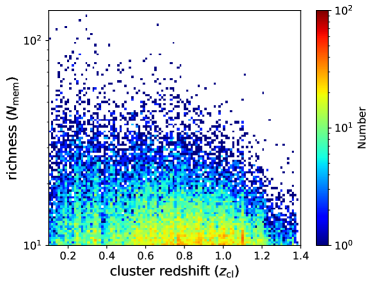
Figure 1: Distributions of cluster redshift ($z_{\rm cl}$) and richness ($N_{\rm mem}$) for the CAMIRA clusters, color-coded by the number of objects per pixel.

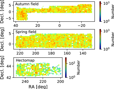
Figure 2: Density maps of CAMIRA member galaxies (top: autumn field, middle: spring field, and bottom: Hectomap).

The redshifts of the member galaxies originate from $z_{\rm spec}$ and photometric redshift ($z_{\rm phot}$). We compiled the values of $z_{\rm spec}$ from literature. such as from the Sloan Digital Sky Survey (SDSS; York et al., 2000) Data Release (DR) 15 (Aguado et al., 2019), Galaxy And Mass Assembly (GAMA; Driver et al., 2011) DR2 (Baldry et al., 2018), DEEP2/3 DR4 (Cooper et al., 2012; Newman et al., 2013), 3D-HST v4.1.5 (Skelton et al., 2014; Momcheva et al., 2016), PRIMUS DR1 (Coil et al., 2011; Cool et al., 2013), VIPERS DR2 (Guzzo et al., 2014; Scodeggio et al., 2018), and VVDS final DR (Le Fèvre et al., 2013) (see also Tanaka et al., 2018; Nishizawa et al., 2020). Furthermore, we employed the Direct Empirical Photometric code (DEmP: Hsieh & Yee, 2014) for member galaxies without $z_{\rm spec}$. DEmP is an empirical quadratic-polynomial photometric-redshift fitting code that exhibits good performance with red-sequence galaxies (see Hsieh et al., 2005; Hsieh & Yee, 2014, for a full description of this redshift code).

Hashiguchi et al. (2023) reported that the $z_{\rm phot}$ of member galaxies could be efficiently estimated with a bias ($\delta_{\rm z}$) of 0.004, a scatter ($\sigma_{\rm z}$) of 0.012, and an outlier rate ($f_{\rm out}$) of 0.008. Because of the involved high quality, we did not herein consider the uncertainty in $z_{\rm phot}$, which exhibits a negligible impact on the final results. If a member galaxy has a value of $z_{\rm spec}$, it is used; otherwise, $z_{\rm phot}$ is used. Hereafter, we refer to the redshift calculated in this manner as $z_{\rm mem}$. We narrowed down the member galaxy sample to sources with $|z_{\rm cl}-z_{\rm mem}|\leq 0.05\times(1+z_{\rm cl})$ for selecting reliable member galaxies (Tanaka et al., 2018, see also Ando et al. 2023). This procedure left 877,642 member galaxies in the CAMIRA clusters, which were used for our subsequent analyses.

2.2 Multiwavelength Dataset

We compiled multiwavelength data from the ultraviolet (UV) to the mid-IR (MIR) range for CAMIRA member galaxies. As described in Section 2.4, this multiwavelength dataset enables us to derive reliable AGN power fractions.

2.2.1 UV Data

For the far-UV (FUV) and near-UV (NUV) data, we utilized the revised catalog (GUVcat_AIS; Bianchi et al., 2017) from the Galaxy Evolution Explorer (GALEX; Martin et al., 2005). This catalog contains 82,992,062 sources with 5$\sigma$ limiting magnitudes of 19.9 and 20.8 for the FUV and NUV, respectively.

We extracted 79,750,759 sources with (i) GRANK $\leq$ 1 and (ii) fuv_artifact = 0 and fuv_flags = 0 or nuv_artifact = 0 and nuv_flags = 0, where GRANK, f/nuv_artifact, and f/nuv_flags are the primary-source, artifact, and extraction flags, respectively. A source with GRANK = 0 has no other sources within 2″.5 while a source with GRANK = 1 is the best source comprising more than one source within this radius. In the GALEX pipeline, the program SExtractor (Bertin & Arnouts, 1996) is used for the detection and photometry of sources in the GALEX. Here, f/nuv_flags contains eight flag bits, with f/nuv_flags = 0 meaning that there are no warnings about the source extraction process. f/nuv_artifact is the bitwise logical ‘OR’, and f/nuv_artifact = 0 implies that a source is unaffected by any artifacts. We refer the reader to Section 6.2 and Appendix A of a paper by Bianchi et al. (2017) and the SExtractor User Manual for more details.

2.2.2 $u$-band Data

Further, we utilized the $u$-band data from the SDSS and Kilo-Degree Survey (KiDS; de Jong et al., 2013). In particular, we used the SDSS PhotoPrimary table in DR17 (Abdurro’uf et al., 2022) and KiDS DR3 (de Jong et al., 2017), which contain 469,053,874 and 48,736,590 sources, respectively. The SDSS survey has a 5$\sigma$ limiting $u$-band magnitude of approximately 22.0, while that of the KiDS survey is approximately 24.3. Because KiDS DR3 does not extend over the entire region covered by the HSC-SSP, we employed the SDSS $u$-band data for objects outside the KiDS footprint. To ensure reliable $u$-band fluxes for KiDS sources, we extracted sources with FLAGS_U = 0 where FLAGS_U is the extraction flag output by SExtractor (Section 2.2.1). If an object lies outside the KiDS footprint, we obtain its $u$-band flux densities based on the SDSS data; otherwise, we refer to the KiDS $u$-band flux. We also checked the consistency between KiDS $u$-band mag ($u_{\rm KiDS}$) and SDSS $u$-band mag ($u_{\rm SDSS}$). The weighted mean of $u_{\rm KiDS}-u_{\rm SDSS}$ is 0.05 mag, indicating that the $u$-band photometry is consistent with the KiDS and SDSS data.

2.2.3 Optical Data

The HSC-SSP survey comprises three layers with different survey depths and areas: wide, deep, and ultradeep layers (Tables 3 and 4 in Aihara et al., 2018b). We used the HSC-SSP s21a wide-layer data obtained between March 2014 and January 2021, which provide forced photometry in the $g$-, $r$-, $i$-, $z$-, and $y$-bands with 5$\sigma$ limiting magnitudes of 26.8, 26.4, 26.4, 25.5, and 24.7, respectively. These photometry data are included in the CAMIRA catalog.

2.2.4 Near-IR Data

We compiled near-IR (NIR) data based on the VISTA Kilo-degree Infrared Galaxy Survey (VIKING; Edge et al., 2013) DR4, containing 94,819,861 sources. We used $J$-, $H$-, and $K_{\rm S}$-band data with 5$\sigma$ limiting magnitudes of approximately $J$ = 21 in Vega magnitude. The VIKING catalog contains the Vega magnitude of each source. We converted these Vega magnitudes into AB magnitudes by employing the offset values $\Delta m$ ($m_{\rm AB}=m_{\rm Vega}+\Delta m$) for the $J$-, $H$-, and $K_{\rm S}$-bands of 0.916, 1.366, and 1.827, respectively, following González-Fernández et al. (2018). Before cross-matching, we extracted 80,580,274 objects with primary_source = 1 and (jpperrbits $<$ 256 or hpperrbits $<$ 256 or kspperrbits $<$ 256) to ensure clean photometry for uniquely detected objects, similar to Toba et al. (2019b).

Because the VIKING DR4 partially covers the HSC-SSP footprint, we employed data from the UKIRT Infrared Deep Sky Survey (UKIDSS; Lawrence et al., 2007) and Two Micron All Sky Survey (2MASS; Skrutskie et al., 2006). We utilized the UKIDSS Large Area Survey DR11plus obtained from the WSA–WFCAM Science Archive, containing 88,298,646 sources. The limiting magnitudes of UKIDSS are 20.2, 19.6, 18.8, and 18.2 Vega magnitudes in the $Y$-, $J$-, $H$-, and $K$-bands, respectively. The UKIDSS catalog lists the Vega magnitudes for each source; subsequently, they are converted into AB magnitudes using offset values $\Delta m$ ($m_{\rm AB}=m_{\rm Vega}+\Delta m$) for the $Y$-, $J$-, $H$-, and $K$-bands of 0.634, 0.938, 1.379, and 1.900, respectively, following Hewett et al. (2006). Before cross-matching, we selected 77,225,762 objects with (priOrSec $\leq$ 0 or = frameSetID) and (jpperrbits $<$ 256 or hpperrbits $<$ 256 or kpperrbits $<$ 256) to ensure clean photometry for uniquely detected objects. For the 2MASS data, we employed the AllWISE catalog (Section 2.2.5) that includes 2MASS photometry. If an object lies outside the VIKING footprint but inside the UKIDSS footprint, we obtain its NIR flux densities based on UKIDSS. If an object lies outside the VIKING footprint and even the UKIDSS footprint, we use 2MASS data. Otherwise, we always refer to the VIKING NIR data.

We evaluated the consistency among the VIKING, UKIDSS, and 2MASS NIR photometry data. For $J$-band, the weighted mean of $J_{\rm UKIDSS}-J_{\rm VIKING}$ and $J_{\rm UKIDSS}-J_{\rm 2MASS}$ is 0.06 and 0.08 mag, respectively. For $H$-band, the weighted mean of $H_{\rm UKIDSS}-H_{\rm VIKING}$ and $H_{\rm UKIDSS}-H_{\rm 2MASS}$ is 0.03 and 0.08 mag, respectively. For $K$-band, the weighted mean of $K_{\rm UKIDSS}-Ks_{\rm VIKING}$ and $K_{\rm UKIDSS}-Ks_{\rm 2MASS}$ is 0.02 and 0.11 mag, respectively. These results indicate that the NIR photometry used herein is broadly consistent with the VIKING, UKIDSS, and 2MASS data.

2.2.5 Mid-IR Data

We obtained MIR data based on the Wide-field Infrared Survey Explorer (WISE; Wright et al., 2010). We utilized the unWISE (Lang, 2014; Schlafly et al., 2019) and AllWISE catalogs (Cutri et al., 2021), which provide 2,214,734,224 and 747,634,026 sources, respectively. The 5$\sigma$ detection limits in the AllWISE catalog are approximately 0.054, 0.071, 0.73, and 5 mJy at 3.4, 4.6, 12, and 22 $\mu$m, respectively. The detection limit in the unWISE catalog is deeper by a factor of 2 at 3.4 and 4.6 $\mu$m. Following Toba et al. (2017b), we extracted 741,753,366 sources from the AllWISE catalog, with (w1sat = 0 and w1cc_map=0), (w2sat = 0 and w2cc_map=0), (w3sat = 0 and w3cc_map = 0), or (w4sat = 0 and w4cc_map = 0) to obtain reliable photometry in each band. The unWISE and AllWISE catalogs contain the Vega magnitude of each source. We converted these Vega magnitudes into AB magnitudes using offset values $\Delta m$ ($m_{\rm AB}=m_{\rm Vega}+\Delta m$) of 2.699, 3.339, 5.174, and 6.620 for 3.4, 4.6, 12, and 22 $\micron$, respectively, following the Explanatory Supplement to the AllWISE Data Release Products. For flux densities in unWISE, we corrected possible contamination from surrounding sources by using frac_flux. Since unWISE 3.4 and 4.6 $\micron$ flux densities are deeper than those of ALLWISE, we basically used unWISE data for 3.4 and 4.6 $\micron$ data while ALLWISE was used for 12 and 22 $\micron$ data.

2.3 Cross-identification of Multiwavelength Data

Finally, multiwavelength data (taken from GALEX, SDSS, KiDS, VIKING, UKIDSS, unWISE, and ALLWISE) were added to the CAMIRA member galaxies by cross-matching each catalog with the CAMIRA member galaxy catalog. We employed 1$\arcsec$ for KiDS, VIKING and SDSS and 3$\arcsec$ for GALEX, unWISE, and AllWISE as a search radius following Toba et al. (2022). Consequently, among 877,642 CAMIRA member galaxies, 8,647 (1.0 %), 263,891 (30.1%), 113,415 (12.9%), 293,360 (33.4%), 347,653 (40.0%), 594,405 (67.7%), and 386,737 (44.1%) objects from GALEX, SDSS, KiDS, VIKING, UKIDSS, unWISE, and AllWISE were identified, respectively. Notably, 478/8,647 (5.5%), 19,629/263,891 (7.4%), 1,718/113,415 (1.5%), 5,716/293,360 (1.9%), 7,738/347,653 (2.2%), 90.748/594,405 (15.2%), and 63,546/386,737 (16.4%) objects had more than two candidate counterparts within the search radius for the GALEX, SDSS, KiDS, VIKING, UKIDSS, unWISE, and AllWISE sources, respectively. We chose the nearest object as the counterpart in these cases. We confirmed that the following results remained unaffected even when the HSC sources with multiple candidate counterparts were discarded during the SED fitting.

2.4 SED Fitting with CIGALE

To derive the AGN power fraction $f_{\rm AGN}$ = $L_{\rm IR}$ (AGNs)/$L_{\rm IR}$, we performed SED fitting. We employed the Code Investigating GALaxy Emission (CIGALE; Burgarella et al., 2005; Noll et al., 2009; Boquien et al., 2019; Yang et al., 2020, 2022). This code allows us to include values for many parameters related to, e.g., the star formation history (SFH), single stellar population, attenuation law, AGN emissions, and dust emissions by considering the energy balance between the UV/optical and IR (see e.g., Buat et al., 2012; Ciesla et al., 2015; Boquien et al., 2016; Lo Faro et al., 2017; Toba et al., 2020a, b; Setoguchi et al., 2021; Toba et al., 2021a; Suleiman et al., 2022; Uematsu et al., 2023; Yamada et al., 2023; Setoguchi et al., 2024; Uematsu et al., 2024). The parameter values used in the SED fitting are presented in Table 2.4.

To find a best-fit SED and estimate physical properties with their uncertainties, CIGALE adopted an analysis module, that is, the so-called pdf_analysis. This module computes the likelihood for all the possible combinations of parameters and generates the probability distribution function for each parameter and each object. Further, it scales the models by a factor ($\alpha$) to obtain physically meaningful values before computing the likelihood. $\alpha$ is described as follows:

$$\alpha=\frac{\sum_{i}\frac{f_{i}m_{i}}{\sigma_{i}^{2}}}{\sum_{i}\frac{m_{i}^{2}}{\sigma_{i}^{2}}}+\frac{\sum_{j}\frac{f_{j}m_{j}}{\sigma_{j}^{2}}}{\sum_{j}\frac{m_{j}^{2}}{\sigma_{j}^{2}}},$$ (1)

where $f_{i}$ and $m_{i}$ are the observed and model flux densities, respectively; $f_{j}$ and $m_{j}$ are the observed and model extensive physical properties, respectively; $\sigma$ is the corresponding uncertainties. The only parameter that is subjected to fitting is the scale factor $\alpha$. Finally, pdf_analysis computes the probability-weighted mean and standard deviation corresponding to the resultant value and its uncertainty for each parameter. An advantage of the methodology adopted in CIGALE is that the models must be computed only once for all the objects because a fixed grid of models is used (see Section 4.3 in Boquien et al., 2019, for a detailed explanation of this module).

Table 1: Parameter values used in SED fitting with CIGALE.

Parameter	Value
Delayed SFH
$\tau_{\rm main}$ (Gyr)	0.1, 0.5, 1.0, 2.0,
	4.0, 6.0, 8.0, 10.0
age (Gyr)	0.1, 0.5, 1.0, 2.0,
	4.0, 6.0, 8.0, 10.0, 12.0
Single Stellar Population (Bruzual & Charlot, 2003)
IMF	Chabrier (2003)
Metallicity	0.02
Dust Attenuation (Calzetti et al., 2000)
$E(B-V)_{\rm line}$	0.05, 0.10, 0.15, 0.20, 0.25,
	0.40, 0.60, 0.80, 1.00, 2.00
AGN Disk +Torus Emission (Stalevski et al., 2016)
$\tau_{\rm 9.7}$	3, 7, 11
$p$	0.5, 1.5
$q$	0.5, 1.5
$\Delta$ (°)	30, 50, 70
$R_{\rm max}/R_{\rm min}$	30
Viewing angle $\theta$ (°)	40
AGN power fraction ($f_{\rm AGN}$)	0.00, 0.05, 0.10, 0.15, 0.20, 0.25,
	0.30, 0.35, 0.40, 0.45, 0.50, 0.55,
	0.60, 0.65, 0.70, 0.75, 0.80, 0.85,
	0.90, 0.95, 0.99
AGN Polar Dust Emission (Yang et al., 2020)
extinction law	SMC
$E(B-V)$	0.0, 0.1, 0.5, 1.0
$T_{\rm dust}^{\rm polar}$ (K)	100
Emissivity $\beta$	1.6
Dust Emission (Dale et al., 2014)
IR power-law slope ($\alpha_{\rm dust}$)	2.0

We adopted a delayed-SFH model by assuming a single starburst with an exponential decay (e.g., Ciesla et al., 2015, 2016), where we parameterized the age of the main stellar population and $e$-folding time of the main stellar population ($\tau_{\rm main}$). We chose the single stellar population model of (Bruzual & Charlot, 2003) by assuming the initial mass function (IMF) of Chabrier (2003) and employed the nebular emission model reported by Inoue (2011) with the implementation of the new CLOUDY HII-region model (Villa-Vélez et al., 2021). For the attenuation of dust associated with the host galaxy, the models proposed by Calzetti et al. (2000) and Leitherer et al. (2002) were used. We parameterized the color excess of the nebular emission lines $E(B-V)_{\rm lines}$, extended using the Leitherer et al. (2002) curve. Additionally, we modeled the reprocessed IR emission of dust absorbed from UV/optical stellar emission considering the dust absorption and emission templates of Dale et al. (2014).

We modeled the AGN emission as emission from an accretion disk and dust torus using SKIRTOR (Stalevski et al., 2016), a clumpy two-phase torus model produced within the framework of the three-dimensional radiative-transfer code SKIRT (Baes et al., 2011; Camps & Baes, 2015). The AGN model in CIGALE comprises seven parameters: the optical depth of the torus at 9.7 $\micron$ ($\tau_{\rm 9.7}$), a torus-density radial parameter ($p$), a torus-density angular parameter ($q$), the angle between the equatorial plane and torus edge ($\Delta$), the ratio between the maximum and minimum torus radii ($R_{\rm max}/R_{\rm min}$), the viewing angle ($\theta$), and the AGN power fraction ($f_{\rm AGN}$). $R_{\rm max}/R_{\rm min}$ and $\theta$ are fixed to be 30 and 40, respectively, to avoid degeneracy of AGN templates (see Yang et al., 2020). Because $f_{\rm AGN}$ is the primary topic of this study, we parameterized it using fine intervals. For the polar dust emission, we assumed a gray body with a dust temperature $T_{\rm dust}^{\rm polar}$ = 100 K and emissivity $\beta$ = 1.6 (e.g., Casey, 2012). We parametrized $E(B-V)$ for the polar dust considering the SMC extinction curve (Prevot et al., 1984).

Under the parameter settings summarized in Table 2.4, we fit the stellar, nebular, AGN, and SF components to at most 15 photometric points (FUV, NUV, $u$, $g$, $r$, $i$, $z$, $y$, $J$, $H$, and $K/Ks$ bands, and 3.4, 4.6, 12, and 22 $\micron$) of 877,642 CAMIRA member galaxies. Figure 3 shows the normalized cumulative histogram of the detected bands, demonstrating that roughly half of the sources have more than eight detected bands for the SED fitting. Even if an object is not detected in a band, we utilize this information by setting 5$\sigma$ upper limits following Toba et al. (2019b) to further constrain the SEDs (Section 3.1). We will discuss how the number of detected bands affects the resultant $f_{\rm AGN}$ in Section 4.1.1.

Notably, the photometry adopted in each catalog is different. As the photometric flux densities are expected to trace the total flux densities, the influence of different photometry methods is likely to be small. Nevertheless, it is worth investigating if physical properties can actually be reliably estimated given the uncertainty of each photometry. This topic will be discussed in Section 4.1.1. We also note that the wavelength coverage of our data is limited to UV–MIR. This is because the energy output is expected to peak in the UV (if unprocessed) and IR (when dust-reprocessed); thus, the dataset we used will be sufficient to estimate the AGN power fraction. However, since some CAMIRA member galaxies are detected by using other wavelengths such as X-ray and radio (Hashiguchi et al., 2023), it is worth investigating how the lack of these data, especially X-ray data, affects the resulting AGN power fraction. This topic will be discussed in Section 4.1.2.

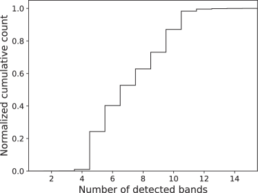
Figure 3: Normalized cumulative histogram of the number of detected bands for CAMIRA member galaxies.

3 Results

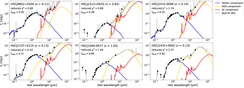
Figure 4: Examples of SED fitting for CAMIRA member galaxies. The black points represent photometric data, while the gray solid line represents the best-fit SED; the contributions of the stellar, AGN, and SF components to the total SED are shown as blue, yellow, and red lines, respectively. The AGN power fraction increases from the top left to bottom right.

3.1 SED Fitting Results

Figure 4 presents examples of SED fitting obtained with CIGALE. The normalized cumulative distribution of reduced $\chi^{2}$ is shown in Figure 5. We confirmed that 756,140 out of 877,642 objects (approximately 86 %) exhibited reduced $\chi^{2}<2.0$, while 789,329 out of 877,642 objects (approximately 90 %) demonstrated reduced $\chi^{2}<3.0$. Those results suggest that the data were moderately well fitted by CIGALE using combination of the stellar, nebular, AGN, and SF components. Meanwhile, notably, approximately 63% of sources have reduced $\chi^{2}<0.5$, which may mean that the data are overfitted and that the estimated uncertainties may be underestimated. In Section 4.1.1, we will discuss how the AGN power fraction of sources with low reduced $\chi^{2}$ are affected. Hereafter, we will focus on the subsample of 756,140 sources with reduced $\chi^{2}<2.0$. We refer to these sources as “CAMIRA AGN power sample (CAMIRA_AP).” In this work, we primarily focus on the AGN power fraction ($f_{\rm AGN}$) of CAMIRA_AP member galaxies. The other AGN properties estimated by CIGALE (i.e., AGN torus-related values) are also provided in Appendix C.

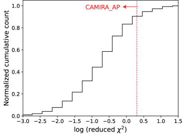
Figure 5: Normalized cumulative histogram of reduced $\chi^{2}$ obtained through SED fitting for CAMIRA member galaxies. The vertical line indicates the reduced $\chi^{2}$ threshold to make a subsample.

3.2 AGN Power Fraction Distribution

In this study, we focused on galaxies that are expected to be member galaxies of clusters by comparing $z_{\rm cl}$ and $z_{\rm mem}$, as outlined in Section 2.1. Notably, the spectroscopic completeness of the CAMIRA_AP member galaxies is considerably low (22,516/756,140 $\sim$ 3.0%); therefore, we relied on $z_{\rm phot}$ for most galaxies. Hence, foreground and background galaxies could possibly contaminate the member galaxies. The CAMIRA catalog assigns a weight factor ($w_{\rm mem}$) to each member galaxy corresponding to its membership probability. This factor is obtained by applying the fast Fourier transform to the two-dimensional richness map containing properties of galaxies (e.g., color and stellar mass). A full description of $w_{\rm mem}$, ranging between 0 and 1, is provided by Oguri (2014). A galaxy with $w_{\rm mem}$ closer to 1 is more likely to be a cluster member galaxy, as evident from its increased membership probability.

Therefore, we employed a membership-probability-weighted AGN power fraction to mitigate the influence of contamination from foreground and background galaxies, as introduced by Bufanda et al. (2017). Because AGN power fraction ($f_{\rm AGN}=L_{\rm IR}$ (AGNs)/$L_{\rm IR}$) can be calculated for each member galaxy and each galaxy is assigned a probability of being a cluster member ($w_{\rm mem}$), the membership-probability-weighted AGN power fraction is defined here in a CAMIRA_AP cluster ($f^{\rm cl}_{\rm AGN}$) as

$$f^{\rm cl}_{\rm AGN}=\frac{\sum w^{i}_{\rm mem}~{}f^{i}_{\rm AGN}}{\sum w^{i}_{\rm mem}},$$ (2)

where $f^{i}_{\rm AGN}$ and $w^{i}_{\rm mem}$ are the AGN power fractions of the $i$-th member galaxy in a CAMIRA_AP cluster and its corresponding membership weight factor, respectively. The uncertainty in $f^{\rm cl}_{\rm AGN}$ is calculated as its standard deviation.

As this work compares $f_{\rm AGN}$ for galaxy clusters with that for field galaxies (Section 3.3), we define the AGN power fraction for field galaxies ($f^{\rm fd}_{\rm AGN}$). For this purpose, we selected 503,595 field galaxies using the HSC-SSP with the same magnitude and color cuts as those used for red-sequence galaxies (Oguri, 2014; Oguri et al., 2018), although the field galaxies do not belong to a cluster. We collected multiwavelength data from the UV–MIR range in exactly the same manner as that discussed in Section 2.2 and estimated $f_{\rm AGN}$ based on SED fitting using the parameter sets described in Section 2.4. The range of the redshift of the field galaxies ($z_{\rm fd}$) is the same as that of the CAMIRA_AP member galaxies. For subsequent analysis, we extracted 371,993 field galaxies by adopting reduced $\chi^{2}<2.0$ from the SED fitting, in the same manner as that adopted for cluster member galaxies (Section 3.1). Because a field galaxy, by definition, does not have $w_{\rm mem}$, we used only field galaxies with $z_{\rm spec}$ and measured the AGN power fraction by weighting the uncertainties of $f_{\rm AGN}$ rather than $w_{\rm mem}$. Hemce $f^{\rm fd}_{\rm AGN}$ is formulated as follows:

$$f^{\rm fd}_{\rm AGN}=\frac{\sum\sigma_{f^{i}_{\rm AGN}}~{}f^{i}_{\rm AGN}}{\sum\sigma_{f^{i}_{\rm AGN}}},$$ (3)

where $f^{i}_{\rm AGN}$ and $\sigma_{f^{i}_{\rm AGN}}$ are the AGN power fractions of the $i$-th field galaxy and its uncertainty, respectively. The uncertainty in $f^{\rm fd}_{\rm AGN}$ is calculated as its standard deviation.

Figure 6 presents the distribution of $f^{\rm cl}_{\rm AGN}$ in CAMIRA_AP clusters. The mean and standard deviations of $f^{\rm cl}_{\rm AGN}$ are 0.39 and 0.06, respectively. We also divided the cluster sample into subsamples based on redshifts ($z_{\rm cl}~{}\leq~{}0.4$, $0.4<z_{\rm cl}~{}\leq~{}0.8$, $0.8<z_{\rm cl}~{}\leq~{}1.2$, and $z_{\rm cl}>1.2$) following Hashiguchi et al. (2023). The numbers of clusters in the redshift bins are 5,193, 10,819, 10,113, and 912, respectively. We examined the $f^{\rm cl}_{\rm AGN}$ distribution of the clusters in each redshift bin (Figure 7). The peak value of the histogram for each panel gradually increases with increasing $z_{\rm cl}$, providing tentative evidence for the redshift dependence of the AGN power fraction (Section 3.3.1 for a quantitative discussion). However, the range of the distribution is relatively large regardless of the redshift, and this should be kept in mind in the subsequent discussion.

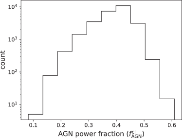
Figure 6: Histogram of the membership-probability-weighted AGN power fraction ($f^{\rm cl}_{\rm AGN}$) for the CAMIRA_AP clusters.

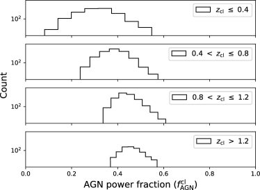
Figure 7: Histograms of the AGN power fraction ($f^{\rm cl}_{\rm AGN}$) for the CAMIRA_AP clusters in each redshift bin.

Figure 8 shows the distribution of $f^{\rm fd}_{\rm AGN}$ of field galaxies in each redshift bin ($z_{\rm fd}\leq 0.4$, $0.4<z_{\rm fd}\leq 0.8$, $0.8<z_{\rm fd}\leq 1.2$, and $z_{\rm fd}>1.2$), and these redshift bins have 98,584, 193,731, 72,849, and 6,829 field galaxies, respectively. The peak value of the histogram for each panel slightly increases with increasing $z_{\rm fd}$; this increase also provides tentative evidence for the redshift dependence of the AGN power fraction even for field galaxies (see Section 3.3.1 for a quantitative discussion). The mean and standard deviations of $f^{\rm fd}_{\rm AGN}$ over the whole redshift range ($0.1<z_{\rm fd}<1.4$) are 0.35 and 0.13, respectively, which are lower than those for galaxy clusters, suggesting that the AGNs may tend to ignite in a dense environment.

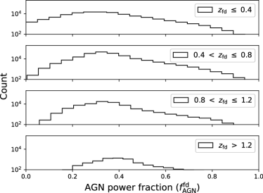
Figure 8: Histograms of the AGN power fraction ($f^{\rm fd}_{\rm AGN}$) for the field galaxies in each redshift bin.

3.3 Redshift and Centric Radius Dependences of the AGN Power Fraction for Galaxy Clusters

We next consider the dependence of the AGN power fraction on (i) redshift and (ii) distance ($R$) from the cluster center (cluster centric radius) scaled using the virial radius ($R_{\rm 200}$), $R/R_{\rm 200}$. Further, we compared the AGN power fraction for clusters with that for field galaxies. Here, we stacked the redshift and radial distributions of member galaxies in redshift or $R/R_{\rm 200}$ bins. We then calculated the AGN power fraction and its uncertainty in each bin by applying the $w_{\rm mem}$ weights, similar to that described in Section 3.2 (Equation 2). Those enabled us to compare the AGN power fraction for clusters to that for field galaxies, as described in Sections 3.3.1 and 3.3.2. Hereafter, we denote the AGN power fraction calculated in this manner as $f^{\rm mem}_{\rm AGN}$.

3.3.1 Redshift Dependence of the AGN Power Fraction

Figure 9 presents the AGN power fraction as a function of redshift. The mean relative error of AGN power fraction across the redshift bin is approximately 0.2%. We verified that $f^{\rm mem}_{\rm AGN}$ increases with increasing redshift, even from an AGN power fraction point of view, similarly to what is reported for the AGN number fraction by previous studies (e.g., Galametz et al., 2009; Martini et al., 2009; Haggard et al., 2010; Hashiguchi et al., 2023). We performed a linear regression to fit the $z_{\rm mem}$–$f^{\rm mem}_{\rm AGN}$ relation considering the uncertainties in each redshift bin. Additionally, we calculated the correlation coefficient ($r$) based on a Bayesian regression method (Kelly, 2007), which yields the correlation coefficient with its corresponding uncertainty (e.g., Toba et al., 2019a, 2021b). The resulting value $r$ = 0.90 $\pm$ 0.14 indicates a strong positive correlation between redshift and AGN power fraction; in other words, a Butcher–Oemler (Butcher & Oemler, 1984)-like effect for AGNs in galaxy clusters was confirmed, even from the perspective of AGN power fraction.

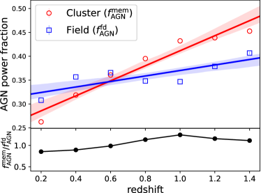
Figure 9: Red circles and blue squares represent the AGN power fractions in the CAMIRA_AP clusters and field, respectively. The vertical error bars are calculated based on the standard deviation of the weighted mean. The mean relative error of the AGN power fraction across the redshift bin is approximately 0.2%. The solid lines with shaded regions represent the best-fit linear regressions with 1$\sigma$ confidence intervals. The bottom panel shows the ratios of $f_{\rm AGN}^{\rm mem}$ and $f_{\rm AGN}^{\rm fd}$.

A positive correlation was found between redshift and AGN number fraction, as has been reported for “field galaxies” by many researchers (e.g., Silverman et al., 2009; Haggard et al., 2010; Oi et al., 2021). Buat et al. (2015) also reported that the AGN power fraction increases with increasing redshift. To determine if this observed trend is specific to the AGNs in clusters or if it merely reflects the trend observed in field galaxies, we calculated the AGN fraction for field galaxies detected using the HSC-SSP.

Figure 9 shows the AGN power fraction for the field galaxies as a function of redshift. We here calculated the AGN power fraction and its uncertainty in each redshift bin by applying the $\sigma_{f_{\rm AGN}}$ weights, similar to that described in Equation 3. An increasing trend of AGN fraction toward a high redshift is also confirmed for field galaxies, with a correlation coefficient of $r=0.66\pm 0.30$. Moreover, we observe that the best-fit slope for clusters is steeper than that for the field, indicating accelerated AGN growth in cluster galaxies with increasing redshift compared to the field, as reported by previous studies (Eastman et al., 2007; Hashiguchi et al., 2023). Average excess ($f^{\rm mem}_{\rm AGN}$/$f^{\rm fd}_{\rm AGN}$) is about 1.2 at $z>0.6$ (bottom panel of Figure 9). Rapidly increasing AGN number fraction at high redshifts has also been reported for MIR-selected AGN (Tomczak et al., 2011; Hashiguchi et al., 2023) (see Section 4.2 in Hashiguchi et al., 2023, for more details). These results suggest that a denser environment (galaxy clusters), particularly in a high-$z$ universe, tends to boost AGN activity.

3.3.2 Cluster Centric Radius Dependences on AGN Power Fraction

Next, we examined the AGN power fraction as a function of the projected distance from the cluster center (cluster centric radius) scaled using $R_{\rm 200}$, $R/R_{\rm 200}$; we determined the cluster centers using centroids of the BCGs identified with the CAMIRA (Oguri et al., 2018). Here, $R_{\rm 200}$ is the radius within which the mass density is 200 times the mean universe mass density. We obtain $R_{\rm 200}$ by assuming the scaling relation between $N_{\rm mem}$ and cluster mass ($M_{\rm 200}$) reported for CAMIRA clusters by Okabe et al. (2019) (see also Murata et al., 2019; Chiu et al., 2020), where $M_{\rm 200}$ is the total mass enclosed within a sphere of radius $R_{\rm 200}$. $R_{\rm 200}$ ranges 0.5–2.5 Mpc for our cluster sample.

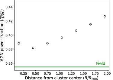
Figure 10: AGN power fraction as a function of cluster centric radius scaled using the virial radius ($R/R_{\rm 200}$). The vertical error bars were calculated based on the standard deviation of the weighted mean. The mean relative error of AGN power fraction across the $R/R_{200}$ bin is about 0.2%. The green-shaded region shows an average AGN power fraction for the field.

Figure 10 shows the resultant $f^{\rm mem}_{\rm AGN}$ as a function of $R/R_{\rm 200}$. We found an excess of $f^{\rm mem}_{\rm AGN}$ at the outskirts of galaxy clusters, which is in good agreement with the results of previous studies (e.g., Khabiboulline et al., 2014; Koulouridis & Bartalucci, 2019). Hashiguchi et al. (2023) also reported that the MIR-selected AGNs are dominant at the outskirts of CAMIRA clusters, while the radio-selected AGNs are condensed to the cluster center. Because the AGN power fraction in this research is based on the IR luminosity, the consistency of our result with that for the MIR-AGNs reported by Hashiguchi et al. (2023) (see also Section 4.1.3) is reasonable.

4 Discussion

4.1 Possible Biases

4.1.1 Mock Analysis

Given the photometric uncertainties, we checked the reliability of the $f_{\rm AGN}$ derived using CIGALE. We performed a mock analysis, which is a procedure provided by CIGALE. This mock analysis was performed by creating a mock catalog. To build the mock catalog, the best-fit value for each object was considered; each quantity was then modified by adding a value taken from a Gaussian distribution with the same standard deviation as the observation uncertainty. Finally, the same method used in the original estimation was applied to obtain mock estimations. Through this analysis, the reliability of the obtained estimations for the physical parameters was estimated. A full description of this process can be found in a paper by Boquien et al. (2019) (see also Ciesla et al., 2015, 2016; Toba et al., 2019b, 2020c; Pouliasis et al., 2022).

Figure 11 shows the differences in the $f_{\rm AGN}$ derived herein using CIGALE and those derived from the mock catalog as a function of redshift and cluster centric radius. The mean (with standard deviation) of $\Delta f_{\rm AGN}$ is $0.08\pm 0.09$, which is acceptable for this research. This result could also suggest that the derived AGN power fraction is not sensitive to the photometric uncertainty. We also proved that $f_{\rm AGN}$ is not considerably dependent on the redshift and distance from the cluster center, indicating that $f_{\rm AGN}$ is well determined with negligible systematic uncertainty.

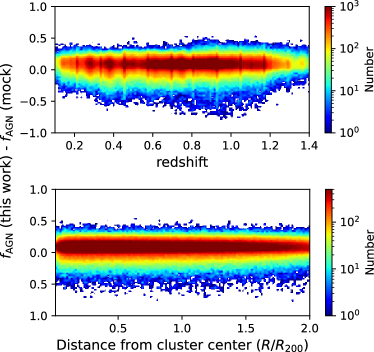
Figure 11: Differences in the $f_{\rm AGN}$ derived herein using CIGALE and those derived using the mock catalog as a function of redshift (top) and distance from the cluster center (bottom); both are color-coded according to the number of objects per pixel.

In Sections 2.4 and 3.1, we reported that the number of detected bands and reduced $\chi^{2}$ obtained through SED fitting have a large variation (Figures 3 and 5). We also tested how the number of detected bands and reduced $\chi^{2}$ depend on $\Delta f_{\rm AGN}$. Figure 12 shows $\Delta f_{\rm AGN}$ as a function of the numbers of detected bands and reduced $\chi^{2}$, demonstrating that $\Delta f_{\rm AGN}$ does not substantially depend on these values. Therefore, we conclude that the limited number of detected bands and threshold of reduced $\chi^{2}$ in this research did not cause systematic uncertainty in the power fraction. This result could also suggest that the influence of the difference in photometry for the SED fitting is likely to be small, as mentioned in Section 2.4.

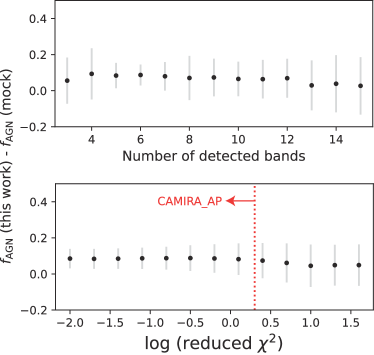
Figure 12: Differences between the $f_{\rm AGN}$ derived herein using CIGALE and the values derived using the mock catalog as a function of number of detected bands (top) and reduced $\chi^{2}$ (bottom).

4.1.2 Lack of X-ray Information

Herein, UV–MIR data were employed to constrain the SED and estimate AGN power fraction, as described in Section 2. However, some CAMIRA member galaxies are detected using other wavelengths, such as those of X-rays and radio waves (Hashiguchi et al., 2023). In particular, X-ray data may be crucial to constrain AGN properties such as $f_{\rm AGN}$, as reported by Yang et al. (2020). Since CIGALE is capable of handling X-ray data, as demonstrated by Yang et al. (2020, 2022), we tested how the lack of X-ray data affects the resultant $f_{\rm AGN}$. For this purpose, we used 263 X-ray-detected CAMIRA member galaxies reported by Hashiguchi et al. (2023), who used XMM-Newton data to identify X-ray sources. We conducted SED fitting to those 263 X-ray sources with and without X-ray flux and compared the calculated AGN power fractions. Figure 13 shows the differences in the AGN power fraction with and without adding X-ray information to SED fitting with CIGALE as a function of X-ray luminosity ($L_{\rm X}$) in the 2–10-keV range, where $L_{\rm X}$ was calculated as shown a study by Hashiguchi et al. (2023). We found that weighted mean and its standard deviation of $f_{\rm AGN}$ (w/ X-ray) - $f_{\rm AGN}$ (wo/ X-ray) is $-0.10\pm 0.04$. We also found that this offset depends on the X-ray luminosity. For a low-luminosity regime, $f_{\rm AGN}$ tends to be overestimated if X-ray information is not used. Meanwhile, for a high-luminosity regime, $f_{\rm AGN}$ tends to be underestimated if X-ray information is not used. These tendencies are in good agreement with those reported by Mountrichas et al. (2021). Thus, we should note the possible systematics of the AGN power fraction in this research.

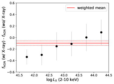
Figure 13: Differences in the AGN power fraction derived using CIGALE with and without X-ray information as a function of X-ray luminosity in the 2–10-keV range. The red solid and dotted lines indicate the weighted mean and standard deviation, respectively, over the X-ray luminosity range of the sample.

4.1.3 Comparisons with the AGN Number Fractions

Hashiguchi et al. (2023) have identified 2,688 AGNs based on multiwavelength data and determined the AGN number fraction for the same initial sample as in this study (i.e., CAMIRA clusters). They have also reported that 2,536 CAMIRA clusters have at least one member galaxy that hosts an AGN. We therefore expected that (i) the member galaxies hosting AGNs in a study by Hashiguchi et al. (2023) will have systematically larger values for $f_{\rm AGN}$ than those without AGNs and (ii) the AGN number fraction for each cluster will be correlated with $f^{\rm cl}_{\rm AGN}$.

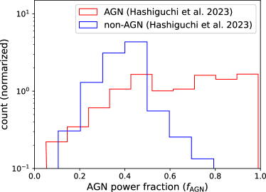
Figure 14: Comparison of $f_{\rm AGN}$ between member galaxies hosting AGNs (red) and those without AGNs (blue) reported by Hashiguchi et al. (2023).

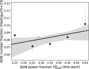
Figure 15: Comparison of the AGN power fraction ($f^{\rm cl}_{\rm AGN}$) obtained herein for each cluster with AGN number fraction reported by Hashiguchi et al. (2023).

Figure 14 compares the distributions of the AGN power fraction (we obtained through SED fitting) for the member galaxies that do and do not host AGNs that were determined by Hashiguchi et al. (2023). We found that the $f_{\rm AGN}$ of AGNs identified by Hashiguchi et al. (2023) is systematically higher than that of objects not identified as AGNs by Hashiguchi et al. (2023), which is supported with $>$99.9% significance by a two-sided Kolmogorov–Smirnov (KS) test. The mean values of $f_{\rm AGN}$ for member galaxies with and without AGNs are 0.63 and 0.23, respectively. Figure 15 compares the AGN number fraction (Hashiguchi et al., 2023) with the AGN power fraction ($f^{\rm cl}_{\rm AGN}$) for each cluster. We confirmed a positive correlation between the AGN number and power fractions, with a correlation coefficient of $r=0.40\pm 0.27$. This implies that as expected, a cluster with high AGN number fraction tends to have high AGN power fraction. We note that about 2% of objects unclassified as AGN by Hashiguchi et al. (2023) have a large AGN power fraction ($f_{\rm AGN}$ $>$ 0.7). Those objects may be good candidates for heavily obscured AGN that were missed by previous surveys.

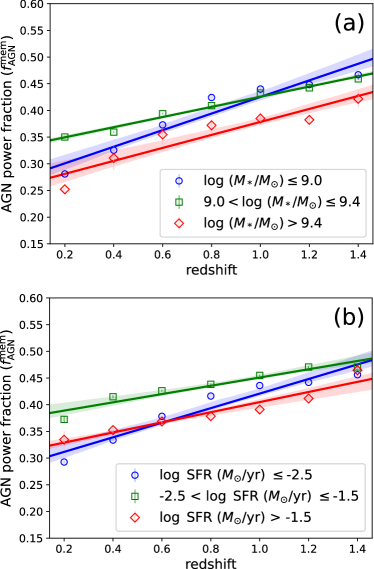
Figure 16: AGN power fraction as a function of redshift for CAMIRA member galaxies with (a) different stellar masses (blue circles: $\log\,(M_{*}/M_{\odot})~{}\leq~{}10.5$, green squares: $10.5<\log\,(M_{*}/M_{\odot})~{}\leq~{}11.5$, and red diamonds: $\log\,(M_{*}/M_{\odot})>11.5$) and (b) different SFR (blue circles: $\log\,{\rm SFR}(M_{\odot}/{\rm yr})~{}\leq~{}-0.5$, green squares: $-0.5<\log\,{\rm SFR}(M_{\odot}/{\rm yr})~{}\leq~{}0.0$, and red diamonds: $\log\,{\rm SFR}(M_{\odot}/{\rm yr})>0.0$). The vertical error bars represent the standard deviation of the weighted mean. The solid lines with shaded regions represent the best-fit linear regressions with 1$\sigma$ confidence intervals.

4.1.4 Stellar Mass and SFR Dependence

We observed a positive correlation between the AGN power fraction and redshift, both for member galaxies in galaxy clusters and those in the field, as discussed in Section 3.3.1. However, some studies have reported that the AGN number fraction depends on the stellar mass ($M_{*}$) of the host galaxy (e.g., Kauffmann et al., 2003; Best et al., 2005; Koss et al., 2011; Bitsakis et al., 2015; Miraghaei, 2020). Because our sample is flux-limited, more massive host galaxies at higher redshifts could exhibit more luminous AGNs, leading to a biased positive correlation between $f_{\rm AGN}$ and redshift. This may also be the case for the SFR because the stellar mass and SFR are often related, and this relation would evolve along with the redshift reported for star-forming galaxies (e.g., Noeske et al., 2007; Schreiber et al., 2015; Pearson et al., 2018).

Following Hashiguchi et al. (2023), we divided our sample into subsamples to investigate how the stellar mass and SFR of member galaxies influence the correlation between the AGN power fraction and redshift. We defined the subsamples using the following ranges of stellar mass: $\log\,(M_{*}/M_{\odot})~{}\leq~{}10.5$, $10.5<\log\,(M_{*}/M_{\odot})~{}\leq~{}11.5$, and $\log\,(M_{*}/M_{\odot})>11.5$; for SFR the range is as follows: $\log\,{\rm SFR}(M_{\odot}/{\rm yr})~{}\leq~{}-0.5$, $-0.5<\log\,{\rm SFR}(M_{\odot}/{\rm yr})~{}\leq~{}0.0$, and $\log\,{\rm SFR}(M_{\odot}/{\rm yr})>0.0$. We obtained $M_{*}$ and SFR from CIGALE outputs, as described in Section 2.4. Figure 16 depicts $f_{\rm AGN}$ as a function of redshift for three subsamples with stellar mass and SFR. We found no significant differences in the correlation coefficients among the subsamples for stellar mass or SFR that were within the respective errors. Hence, we concluded that the observed positive correlation of $z_{\rm cl}$–$f^{\rm mem}_{\rm AGN}$ was not affected by such biases.

4.2 Cluster Mass Dependence on AGN Power Fraction

We also investigated how the AGN power fraction depends on $M_{\rm 200}$ (or richness). As shown in Figure 17, the AGN power fraction decreases with increasing $M_{\rm 200}$, with the correlation coefficient being $r=-0.91\pm 0.14$. This trend is in good agreement with the results of previous studies (e.g., Koulouridis et al., 2018; Noordeh et al., 2020; Hashiguchi et al., 2023). It was also observed in a study by Popesso & Biviano (2006), who reported an anticorrelation between the AGN number fraction and velocity dispersion of galaxy clusters. Because the velocity dispersion of a galaxy cluster can be translated into $M_{\rm 200}$ (e.g., Smith, 1936); this provides additional support for our findings. These results suggest that a galaxy in a group environment is more likely to ignite an AGN than a cluster environment, which is consistent with previous studies by Li et al. (2019), Pentericci et al. (2013), and Hashiguchi et al. (2023).

In addition, we examined how the AGN power fraction depends on the cluster centric radius in different $M_{\rm 200}$ ranges (Figure 18). Notably, massive clusters tend to be responsible for the rapid increase in the AGN power fraction at the cluster outskirts, as reported in Section 3.3.2. We further discuss this point in Section 4.3, considering the morphologies of the galaxy clusters.

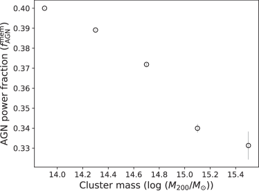
Figure 17: AGN power fraction as a function of cluster mass ($M_{\rm 200}$). The vertical error bars represent the standard deviations of the weighted means.

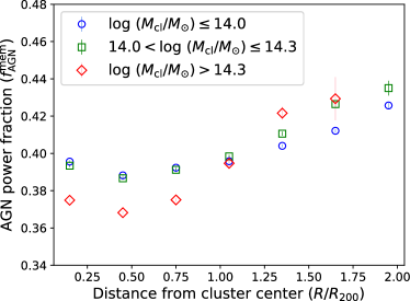
Figure 18: AGN power fraction as a function of cluster centric radius scaled using the virial radius ($R/R_{\rm 200}$) for different cluster mass ranges (blue diamonds: $\log\,(M_{\rm cl}/M_{\odot})$ $\leq$ 14.0, green squares: $14.0<\log\,(M_{\rm cl}/M_{\odot})$ $\leq$ 14.3, and red diamonds: $\log\,(M_{\rm cl}/M_{\odot})>14.3$). The vertical error bars represent the standard deviations of the weighted means.

4.3 Cluster Morphology Dependence on AGN Power Fraction

We next consider how the emergence of AGNs depends on the substructure and morphology of galaxy clusters. Okabe et al. (2019) identified merging-cluster candidates based on the CAMIRA cluster catalog using a peak-finding method. This method involves counting the number of peaks above a redshift-dependent threshold based on Gaussian-smoothed maps of the number densities of member galaxies. A galaxy cluster with a single peak was classified as a “relaxed” cluster, while a cluster with more than two peaks was considered a “merging” cluster. Accordingly, they classified 2,558 out of 27,037 CAMIRA clusters (approximately 9.5%) as merging clusters, with 150,684 member galaxies associated with them.

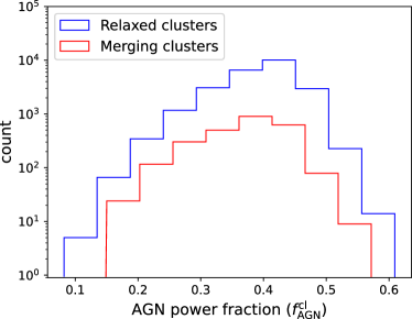
Figure 19: $f^{\rm cl}_{\rm AGN}$ distributions for relaxed (blue) and merging (red) clusters.

Figure 19 presents the distribution of $f^{\rm cl}_{\rm AGN}$ for relaxed and merging clusters. There was no significant difference between the two clusters, as we confirmed this with $>$99.9% significance using a two-sided KS test. This result suggests that cluster–cluster mergers may not necessarily trigger AGNs, as also reported by Silva et al. (2021); Hashiguchi et al. (2023). The dynamical activity within a cluster may also activate SF activity in member galaxies (e.g., Miller & Owen, 2003; Sobral et al., 2015; Stroe et al., 2015; Okabe et al., 2019). Stroe & Sobral (2021) recently reported that a large fraction of emission-line galaxies in merging clusters are powered by star formation rather than by AGNs. On the other hand, Noordeh et al. (2020) suggested that merging-cluster environments may contribute to the enhancement of AGN activity. Several enhancement mechanisms have been proposed for SF and AGN activity in merging clusters, including gas incorporation driven by ram pressure and galaxy–galaxy interactions (Treu et al., 2003, and references therein). The relative strengths of SF and AGN may depend on the abovementioned dominant mechanism and the sequence of cluster–cluster mergers. Future statistical work that considers the merger stage of a cluster–cluster merger may provide a way to resolve this issue.

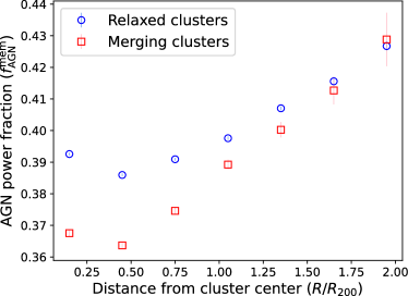
Figure 20: AGN power fraction as a function of cluster centric radius scaled using the virial radius ($R/R_{\rm 200}$) for relaxed (blue circles) and merging (red squares) clusters.

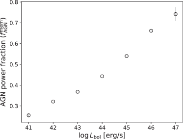
Figure 21: AGN power fraction as a function of bolometric luminosity.

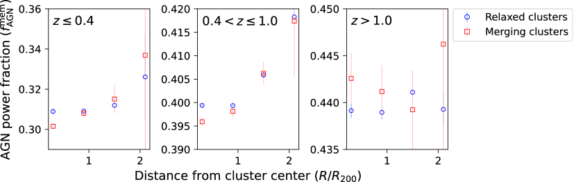
Figure 22: AGN power fraction as a function of cluster centric radius scaled using the virial radius ($R/R_{\rm 200}$) for relaxed (blue circles) and merging (red squares) clusters in each redshift bin.

Figure 20 illustrates the cluster centric radius dependence of the AGN fraction for relaxed and merging clusters. We found that AGNs were enhanced in relaxed clusters and that cluster–cluster mergers may not lead to increased AGN activity in the cluster center. The member galaxies may be moving too quickly to interact with each other, particularly in the cluster center, even if a cluster–cluster merger has occurred. We also found that AGNs are more likely to be enhanced at the outskirts of merging clusters rather than relaxed ones. These findings are in good agreement with those obtained from the AGN number fraction (Hashiguchi et al., 2023). The suppression of AGN activity at the cluster center of the merging clusters was also reported by a cosmological simulation (Chadayammuri et al., 2021). Figure 22 illustrates the cluster centric radius dependence of the AGN fraction for relaxed and merging clusters in some redshift bins ($z\leq 0.4$, $0.4<z\leq 1.0$, and $z>1.0$). The observed trend seen in Figure 20 seems to be established at $z\leq 1.0$. Although the AGNs may be enhanced even in the cluster center in merging clusters at $z>1.0$, we need more samples to confirm this possibility.

Because the AGN activity in massive clusters may be enhanced in the outskirts of clusters (as mentioned in Section 4.2), merging clusters with larger $M_{\rm 200}$ values are more likely to experience increased AGN activity in their outskirts. Notably, the fraction of AGNs in galaxy–galaxy mergers increases with increasing luminosity (e.g., Treister et al., 2012; Glikman et al., 2015; Dietrich et al., 2018; Weigel et al., 2018). We tested how the AGN power fraction depends on AGN bolometric luminosity ($L_{\rm bol}$). To estimate $L_{\rm bol}$, we integrated the best-fit SED template of the AGN component output by CIGALE over wavelengths longward of Ly$\alpha$ in the same manner as that performed by Toba et al. (2017a). Figure 21 shows the AGN power fraction as a function of AGN bolometric luminosity for CAMIRA_AP member galaxies. We found that $f_{\rm AGN}$ is strongly correlated with $L_{\rm bol}$ with a correlation coefficient of $r=0.97\pm 0.07$. This result supports the idea that luminous AGNs can be enhanced in a dense environment, thereby merging clusters.

We note that the optical center of a cluster does not always correspond to the peak galaxy density, and it may also significantly differ from the X-ray center in certain instances, as reported by various researchers, including Mahdavi et al. (2013), Oguri et al. (2018), and Ota et al. (2023). This effect may be more severe when clusters merge. Although the fraction of merging clusters was small in the present study, this effect could impact the overall trend discussed in Section 3.3.2. It is therefore important to consider the potential uncertainty in $R$ for merging clusters.

4.4 AGN Feedback to SFR in Galaxy Clusters

Finally, we discuss how the AGN power fraction depends on the SFR of CAMIRA_AP member galaxies and field galaxies. Figure 23 depicts the AGN power fraction as a function of SFR for member galaxies of clusters and field galaxies. The AGN power fraction of field galaxies ($f^{\rm fd}_{\rm AGN}$) does not exhibit any remarkable SFR dependence. In contrast, the AGN power fraction of CAMIRA_AP member galaxies ($f^{\rm mem}_{\rm AGN}$) rapidly decreases when $\log\,{\rm SFR}>0$. In other words, when the AGN power fraction is high, the SFR tends to be small, possibly implying that the AGN feedback quenches the SF activity in member galaxies of the cluster. This implication suggests that AGN feedback (such as gas-heating and outflow by AGN) is more effective in dense environments (see also Boselli et al., 2016; Maier et al., 2022; Peluso et al., 2022).

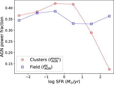
Figure 23: AGN power fraction as a function of SFR for member galaxies in CAMIRA_AP clusters (red circles) and field galaxies (blue squares).

5 Summary

We have investigated how AGN activity depends on the environment—in particular, on $z_{\rm cl}$ and the distance from the cluster center—from an AGN-energy-contribution point of view. Following Hashiguchi et al. (2023), we utilized one of the largest optically selected galaxy cluster catalogs: the CAMIRA clusters selected with the Subaru HSC. For approximately one million member galaxies of CAMIRA clusters in the redshift range $0.1<z_{\rm cl}<1.4$, we collected multiwavelength data from the UV-MIR range and have performed SED fitting to determine the AGN power fractions. To mitigate against possible contamination from foreground and background galaxies, we introduced a membership-probability-weighted AGN power fraction and determined how this value depends on $z_{\rm cl}$ and cluster centric radius. Our primary findings are as follows:

• In agreement with recent studies based on the AGN number fraction, we find that the AGN power fraction increases with increasing redshift for cluster members and field galaxies. In addition, the AGN power fraction for galaxy clusters increases more rapidly than for field galaxies (Section 3.3.1).

• The AGN power fraction increases toward the outskirts of galaxy clusters, which is consistent with the results reported by Hashiguchi et al. (2023) based on the number fraction of IR-selected AGNs. In contrast, the AGN power fraction decreases with increasing $M_{\rm 200}$, suggesting that AGN formation may be favored in galaxy group (Sections 3.3.2 and 4.2).

• Although the centers of merging clusters may be somewhat uncertain, we find that cluster–cluster mergers may not be the primary trigger for AGN activity in member galaxies. However, a cluster–cluster merger may enhance AGN formation at the outskirts of a cluster, especially for massive galaxy clusters (Section 4.3).

• We have tentative evidence of AGN negative feedback in clusters, suggesting that AGN could suppress SF activity of member galaxies in denser environments (Section 4.4).

These results indicate that the emergence of an AGN population is influenced by its environment and redshift and that galaxy groups and clusters at high redshifts are perhaps crucial in AGN evolution. However, most CAMIRA cluster members have not yet been spectroscopically confirmed. Future spectroscopic studies using next-generation multiobject spectrographs—such as the Subaru Prime Focus Spectrograph (PFS: Takada et al., 2014, see also Greene et al. 2022)—will help to resolve this issue and provide more-robust conclusions.

Appendix A Value-added CAMIRA member galaxy catalog

We provide the physical properties of 877,642 CAMIRA member galaxies at $0<z_{\rm cl}<1.4$. The catalog description is summarized in Table 2.

Table 2: Physical properties of 877,642 CAMIRA member galaxies at $0<z_{\rm cl}<1.4$.

Column name	Format	Unit	Description
ID_cl	LONG64		Unique id
Name_cl	STRING		Object name
z_cl	FLOAT		Cluster redshift (Oguri et al., 2018)
N_mem	FLOAT		Richness (Oguri et al., 2018)
log_M200	FLOAT	$M_{\sun}$	Cluster mass (Okabe et al., 2019)
Flag_cl_multi_peaks	BOOLEAN		True (multiple peaks), False (single peak) (Okabe et al., 2019)
			In this work, a galaxy cluster with a single peak is classified as a relaxed cluster,
			while a cluster with multiple peaks is considered a merging cluster (Section 4.3).
ID	LONG64		Unique id for member galaxies
Name	STRING		Object name
R.A.	DOUBLE	degree	Right Assignation (J2000.0) from the HSC s21a_wide
Decl.	DOUBLE	degree	Declination (J2000.0) from the HSC s21a_wide
z_mem	FLOAT		Redshift (Section 2.1)
R_R200	FLOAT		Projected distance from the cluster center scaled using the virial radius
$u$mag	FLOAT	AB mag.	$u$-band magnitude
$u$mag_err	FLOAT	AB mag.	$u$-band magnitude error
$g$mag	FLOAT	AB mag.	$g$-band magnitude
$g$mag_err	FLOAT	AB mag.	$g$-band magnitude error
$r$mag	FLOAT	AB mag.	$r$-band magnitude
$r$mag_err	FLOAT	AB mag.	$r$-band magnitude error
$i$mag	FLOAT	AB mag.	$i$-band magnitude
$i$mag_err	FLOAT	AB mag.	$i$-band magnitude error
$z$mag	FLOAT	AB mag.	$z$-band magnitude
$z$mag_err	FLOAT	AB mag.	$z$-band magnitude error
$y$mag	FLOAT	AB mag.	$y$-band magnitude
$y$mag_err	FLOAT	AB mag.	$y$-band magnitude error
$j$mag	FLOAT	AB mag.	$J$-band magnitude
$j$mag_err	FLOAT	AB mag.	$J$-band magnitude error
$h$mag	FLOAT	AB mag.	$H$-band magnitude
$h$mag_err	FLOAT	AB mag.	$H$-band magnitude error
$k$mag	FLOAT	AB mag.	$K$-band magnitude
$k$mag_err	FLOAT	AB mag.	$K$-band magnitude error
Flux_34	FLOAT	mJy	Flux density at 3.4 $\micron$
Flux_34_err	FLOAT	mJy	Uncertainty of flux density at 3.4 $\micron$
Flux_46	FLOAT	mJy	Flux density at 4.6 $\micron$
Flux_46_err	FLOAT	mJy	Uncertainty of flux density at 4.6 $\micron$
Flux_12	FLOAT	mJy	Flux density at 12 $\micron$
Flux_12_err	FLOAT	mJy	Uncertainty of flux density at 12 $\micron$
Flux_22	FLOAT	mJy	Flux density at 22 $\micron$ flux density
Flux_22_err	FLOAT	mJy	Uncertainty of flux density at 22 $\micron$
Flag_upper_limit_u	BOOLEAN		Upper limit flag for $u$mag. True (5$\sigma$ upper limit), False (otherwise)
Flag_upper_limit_g	BOOLEAN		Upper limit flag for $g$mag. True (5$\sigma$ upper limit), False (otherwise)
Flag_upper_limit_r	BOOLEAN		Upper limit flag for $r$mag. True (5$\sigma$ upper limit), False (otherwise)
Flag_upper_limit_i	BOOLEAN		Upper limit flag for $i$mag. True (5$\sigma$ upper limit), False (otherwise)
Flag_upper_limit_z	BOOLEAN		Upper limit flag for $z$mag. True (5$\sigma$ upper limit), False (otherwise)
Flag_upper_limit_y	BOOLEAN		Upper limit flag for $y$mag. True (5$\sigma$ upper limit), False (otherwise)
Flag_upper_limit_J	BOOLEAN		Upper limit flag for $J$mag. True (5$\sigma$ upper limit), False (otherwise)
Flag_upper_limit_H	BOOLEAN		Upper limit flag for $H$mag. True (5$\sigma$ upper limit), False (otherwise)
Flag_upper_limit_K	BOOLEAN		Upper limit flag for $K$mag. True (5$\sigma$ upper limit), False (otherwise)
Flag_upper_limit_34	BOOLEAN		Upper limit flag for Flux_34. True (5$\sigma$ upper limit), False (otherwise)
Flag_upper_limit_46	BOOLEAN		Upper limit flag for Flux_46. True (5$\sigma$ upper limit), False (otherwise)
Flag_upper_limit_12	BOOLEAN		Upper limit flag for Flux_12. True (5$\sigma$ upper limit), False (otherwise)
Flag_upper_limit_22	BOOLEAN		Upper limit flag for Flux_22. True (5$\sigma$ upper limit), False (otherwise)
rchi2	FLOAT		Reduced $\chi^{2}$ obtained from CIGALE
Flag_CAMIRA_AP	BOOLEAN		True (CAMIRA_AP sample), False (otherwise) (Section 3.1)
E_BV	FLOAT		Color excess ($E(B-V)$) derived from CIGALE
E_BV_err	FLOAT		Uncertainty of color excess ($E(B-V)$) derived from CIGALE
log_M	FLOAT	$M_{\sun}$	Stellar mass derived from CIGALE
log_M_err	FLOAT	$M_{\sun}$	Uncertainty of stellar mass derived from CIGALE
log_SFR	FLOAT	$M_{\sun}$ yr${}^{-1}$	SFR derived from CIGALE
log_SFR_err	FLOAT	$M_{\sun}$ yr${}^{-1}$	Uncertainty of SFR derived from CIGALE
log_LIR	FLOAT	$L_{\sun}$	IR luminosity derived from CIGALE
log_LIR_err	FLOAT	$L_{\sun}$	Uncertainty of IR luminosity derived from CIGALE
log_LIR_AGN	FLOAT	$L_{\sun}$	IR luminosity contributed from AGNs derived from CIGALE
log_LIR_AGN_err	FLOAT	$L_{\sun}$	Uncertainty of log_LIR_AGN derived from CIGALE
f_AGN	FLOAT		AGN power fraction (i.e., log_LIR_AGN/log_LIR)
f_AGN_err	FLOAT		Uncertainty of AGN power fraction
Flag_AGN	STRING		IR (IR-AGNs), Radio (Radio-AGNs), X (X-ray AGNs) (Hashiguchi et al., 2023)

Note. — The entire table is available in a machine-readable form in the online journal.

Appendix B Best-fit SED for each CAMIRA member galaxy

The best-fit SED derived from CIGALE is available in Table 3. We encourage using a template of objects with reduced $\chi^{2}<$ 2.0 for science (Section 3.1).

Table 3: Best-fit SED template of each CAMIRA member galaxy.

Column name	Format	Unit	Description
ID	LONG		Unique id for member galaxies
Wavelength	DOUBLE	$\micron$	Wavelength (observed frame)
FNU	DOUBLE	mJy	Flux density at each wavelength
LNU	DOUBLE	W	Luminosity density at each wavelength

Note. — The entire table is available in a machine-readable form in the online journal.

Appendix C Other AGN properties of CAMIRA member galaxies

This work highlights AGN power fraction as a representative AGN property of the CAMIRA_AP member galaxies. We also derive other AGN properties primarily related to the torus AGN structure through SED fitting using CIGALE, as described in Section 3.1. Herein, we present four quantities of the CAMIRA_AP member galaxies: optical depth of the torus at 9.7 $\micron$ ($\tau_{\rm 9.7}$), torus-density radial parameter ($p$), torus-density angular parameter ($q$), and viewing angle ($\theta$). Figure 24 shows the histograms of the four quantities, which are broadly distributed. The weighted mean values of $\tau_{\rm 9.7}$, $p$, $q$, and $\theta$ are 7.10, 1.00, 0.99, and 52.2, respectively. Notably, because the input parameter values of the quantities are sparser than those of the AGN power fraction (Table 2.4), herein, the relative errors are considerably large (30%–50%).

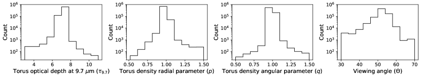
Figure 24: Distributions of the AGN-related physical properties (except for the AGN power fraction) obtained through SED fitting using CIGALE.

References

- Abdurro’uf et al. (2022) Abdurro’uf, Accetta, K., Aerts, C., et al. 2022, ApJS, 259, 35, doi: 10.3847/1538-4365/ac4414
- Aguado et al. (2019) Aguado, D. S., Ahumada, R., Almeida, A., et al. 2019, ApJS, 240, 23, doi: 10.3847/1538-4365/aaf651
- Aihara et al. (2018a) Aihara, H., Armstrong, R., Bickerton, S., et al. 2018a, PASJ, 70, S8, doi: 10.1093/pasj/psx081
- Aihara et al. (2018b) Aihara, H., Arimoto, N., Armstrong, R., et al. 2018b, PASJ, 70, S4, doi: 10.1093/pasj/psx066
- Aihara et al. (2019) Aihara, H., AlSayyad, Y., Ando, M., et al. 2019, PASJ, 71, 114, doi: 10.1093/pasj/psz103
- Aihara et al. (2022) —. 2022, PASJ, 74, 247, doi: 10.1093/pasj/psab122
- Ando et al. (2023) Ando, M., Shimasaku, K., & Ito, K. 2023, MNRAS, 519, 13, doi: 10.1093/mnras/stac3251
- Assef et al. (2018) Assef, R. J., Stern, D., Noirot, G., et al. 2018, ApJS, 234, 23, doi: 10.3847/1538-4365/aaa00a
- Astropy Collaboration et al. (2013) Astropy Collaboration, Robitaille, T. P., Tollerud, E. J., et al. 2013, A&A, 558, A33, doi: 10.1051/0004-6361/201322068
- Astropy Collaboration et al. (2018) Astropy Collaboration, Price-Whelan, A. M., Sipőcz, B. M., et al. 2018, AJ, 156, 123, doi: 10.3847/1538-3881/aabc4f
- Astropy Collaboration et al. (2022) Astropy Collaboration, Price-Whelan, A. M., Lim, P. L., et al. 2022, apj, 935, 167, doi: 10.3847/1538-4357/ac7c74
- Baes et al. (2011) Baes, M., Verstappen, J., De Looze, I., et al. 2011, ApJS, 196, 22, doi: 10.1088/0067-0049/196/2/22
- Baldry et al. (2018) Baldry, I. K., Liske, J., Brown, M. J. I., et al. 2018, MNRAS, 474, 3875, doi: 10.1093/mnras/stx3042
- Bertin & Arnouts (1996) Bertin, E., & Arnouts, S. 1996, A&AS, 117, 393, doi: 10.1051/aas:1996164
- Best et al. (2005) Best, P. N., Kauffmann, G., Heckman, T. M., et al. 2005, MNRAS, 362, 25, doi: 10.1111/j.1365-2966.2005.09192.x
- Bhargava et al. (2023) Bhargava, S., Garrel, C., Koulouridis, E., et al. 2023, A&A, 673, A92, doi: 10.1051/0004-6361/202244898
- Bianchi et al. (2017) Bianchi, L., Shiao, B., & Thilker, D. 2017, ApJS, 230, 24, doi: 10.3847/1538-4365/aa7053
- Bitsakis et al. (2015) Bitsakis, T., Dultzin, D., Ciesla, L., et al. 2015, MNRAS, 450, 3114, doi: 10.1093/mnras/stv755
- Boquien et al. (2019) Boquien, M., Burgarella, D., Roehlly, Y., et al. 2019, A&A, 622, A103, doi: 10.1051/0004-6361/201834156
- Boquien et al. (2016) Boquien, M., Kennicutt, R., Calzetti, D., et al. 2016, A&A, 591, A6, doi: 10.1051/0004-6361/201527759
- Bosch et al. (2018) Bosch, J., Armstrong, R., Bickerton, S., et al. 2018, PASJ, 70, S5, doi: 10.1093/pasj/psx080
- Boselli et al. (2016) Boselli, A., Roehlly, Y., Fossati, M., et al. 2016, A&A, 596, A11, doi: 10.1051/0004-6361/201629221
- Bruzual & Charlot (2003) Bruzual, G., & Charlot, S. 2003, MNRAS, 344, 1000, doi: 10.1046/j.1365-8711.2003.06897.x
- Buat et al. (2012) Buat, V., Noll, S., Burgarella, D., et al. 2012, A&A, 545, A141, doi: 10.1051/0004-6361/201219405
- Buat et al. (2015) Buat, V., Oi, N., Heinis, S., et al. 2015, A&A, 577, A141, doi: 10.1051/0004-6361/201425399
- Bufanda et al. (2017) Bufanda, E., Hollowood, D., Jeltema, T. E., et al. 2017, MNRAS, 465, 2531, doi: 10.1093/mnras/stw2824
- Burgarella et al. (2005) Burgarella, D., Buat, V., & Iglesias-Páramo, J. 2005, MNRAS, 360, 1413, doi: 10.1111/j.1365-2966.2005.09131.x
- Butcher & Oemler (1984) Butcher, H., & Oemler, A., J. 1984, ApJ, 285, 426, doi: 10.1086/162519
- Calzetti et al. (2000) Calzetti, D., Armus, L., Bohlin, R. C., et al. 2000, ApJ, 533, 682, doi: 10.1086/308692
- Camps & Baes (2015) Camps, P., & Baes, M. 2015, Astronomy and Computing, 9, 20, doi: 10.1016/j.ascom.2014.10.004
- Casey (2012) Casey, C. M. 2012, MNRAS, 425, 3094, doi: 10.1111/j.1365-2966.2012.21455.x
- Chabrier (2003) Chabrier, G. 2003, PASP, 115, 763, doi: 10.1086/376392
- Chadayammuri et al. (2021) Chadayammuri, U., Tremmel, M., Nagai, D., Babul, A., & Quinn, T. 2021, MNRAS, 504, 3922, doi: 10.1093/mnras/stab1010
- Chambers et al. (2016) Chambers, K. C., Magnier, E. A., Metcalfe, N., et al. 2016, ArXiv e-prints. https://arxiv.org/abs/1612.05560
- Chiu et al. (2020) Chiu, I. N., Umetsu, K., Murata, R., Medezinski, E., & Oguri, M. 2020, MNRAS, 495, 428, doi: 10.1093/mnras/staa1158
- Ciesla et al. (2015) Ciesla, L., Charmandaris, V., Georgakakis, A., et al. 2015, A&A, 576, A10, doi: 10.1051/0004-6361/201425252
- Ciesla et al. (2016) Ciesla, L., Boselli, A., Elbaz, D., et al. 2016, A&A, 585, A43, doi: 10.1051/0004-6361/201527107
- Coil et al. (2011) Coil, A. L., Blanton, M. R., Burles, S. M., et al. 2011, ApJ, 741, 8, doi: 10.1088/0004-637X/741/1/8
- Cool et al. (2013) Cool, R. J., Moustakas, J., Blanton, M. R., et al. 2013, ApJ, 767, 118, doi: 10.1088/0004-637X/767/2/118
- Cooper et al. (2012) Cooper, M. C., Griffith, R. L., Newman, J. A., et al. 2012, MNRAS, 419, 3018, doi: 10.1111/j.1365-2966.2011.19938.x
- Coupon et al. (2018) Coupon, J., Czakon, N., Bosch, J., et al. 2018, PASJ, 70, S7, doi: 10.1093/pasj/psx047
- Cutri et al. (2021) Cutri, R. M., Wright, E. L., Conrow, T., et al. 2021, VizieR Online Data Catalog, II/328
- Dale et al. (2014) Dale, D. A., Helou, G., Magdis, G. E., et al. 2014, ApJ, 784, 83, doi: 10.1088/0004-637X/784/1/83
- de Jong et al. (2013) de Jong, J. T. A., Verdoes Kleijn, G. A., Kuijken, K. H., & Valentijn, E. A. 2013, Experimental Astronomy, 35, 25, doi: 10.1007/s10686-012-9306-1
- de Jong et al. (2017) de Jong, J. T. A., Verdoes Kleijn, G. A., Erben, T., et al. 2017, A&A, 604, A134, doi: 10.1051/0004-6361/201730747
- Dietrich et al. (2018) Dietrich, J., Weiner, A. S., Ashby, M. L. N., et al. 2018, MNRAS, 480, 3562, doi: 10.1093/mnras/sty2056
- Driver et al. (2011) Driver, S. P., Hill, D. T., Kelvin, L. S., et al. 2011, MNRAS, 413, 971, doi: 10.1111/j.1365-2966.2010.18188.x
- Eastman et al. (2007) Eastman, J., Martini, P., Sivakoff, G., et al. 2007, ApJ, 664, L9, doi: 10.1086/520577
- Edge et al. (2013) Edge, A., Sutherland, W., Kuijken, K., et al. 2013, The Messenger, 154, 32
- Ehlert et al. (2014) Ehlert, S., von der Linden, A., Allen, S. W., et al. 2014, MNRAS, 437, 1942, doi: 10.1093/mnras/stt2025
- Ellison et al. (2008) Ellison, S. L., Patton, D. R., Simard, L., & McConnachie, A. W. 2008, AJ, 135, 1877, doi: 10.1088/0004-6256/135/5/1877
- Fabian (2012) Fabian, A. C. 2012, ARA&A, 50, 455, doi: 10.1146/annurev-astro-081811-125521
- Ferrarese & Merritt (2000) Ferrarese, L., & Merritt, D. 2000, ApJ, 539, L9, doi: 10.1086/312838
- Furusawa et al. (2018) Furusawa, H., Koike, M., Takata, T., et al. 2018, PASJ, 70, S3, doi: 10.1093/pasj/psx079
- Galametz et al. (2009) Galametz, A., Stern, D., Eisenhardt, P. R. M., et al. 2009, ApJ, 694, 1309, doi: 10.1088/0004-637X/694/2/1309
- Glikman et al. (2015) Glikman, E., Simmons, B., Mailly, M., et al. 2015, ApJ, 806, 218, doi: 10.1088/0004-637X/806/2/218
- González-Fernández et al. (2018) González-Fernández, C., Hodgkin, S. T., Irwin, M. J., et al. 2018, MNRAS, 474, 5459, doi: 10.1093/mnras/stx3073
- Greene et al. (2022) Greene, J., Bezanson, R., Ouchi, M., Silverman, J., & the PFS Galaxy Evolution Working Group. 2022, arXiv e-prints, arXiv:2206.14908, doi: 10.48550/arXiv.2206.14908
- Guzzo et al. (2014) Guzzo, L., Scodeggio, M., Garilli, B., et al. 2014, A&A, 566, A108, doi: 10.1051/0004-6361/201321489
- Haggard et al. (2010) Haggard, D., Green, P. J., Anderson, S. F., et al. 2010, ApJ, 723, 1447, doi: 10.1088/0004-637X/723/2/1447
- Harris et al. (2020) Harris, C. R., Millman, K. J., van der Walt, S. J., et al. 2020, Nature, 585, 357, doi: 10.1038/s41586-020-2649-2
- Hashiguchi et al. (2023) Hashiguchi, A., Toba, Y., Ota, N., et al. 2023, PASJ, 75, 1246, doi: 10.1093/pasj/psad066
- Hewett et al. (2006) Hewett, P. C., Warren, S. J., Leggett, S. K., & Hodgkin, S. T. 2006, MNRAS, 367, 454, doi: 10.1111/j.1365-2966.2005.09969.x
- Hsieh & Yee (2014) Hsieh, B. C., & Yee, H. K. C. 2014, ApJ, 792, 102, doi: 10.1088/0004-637X/792/2/102
- Hsieh et al. (2005) Hsieh, B. C., Yee, H. K. C., Lin, H., & Gladders, M. D. 2005, ApJS, 158, 161, doi: 10.1086/429293
- Huang et al. (2018) Huang, S., Leauthaud, A., Murata, R., et al. 2018, PASJ, 70, S6, doi: 10.1093/pasj/psx126
- Hunter (2007) Hunter, J. D. 2007, Computing in science & engineering, 9, 90
- Inoue (2011) Inoue, A. K. 2011, MNRAS, 415, 2920, doi: 10.1111/j.1365-2966.2011.18906.x
- Ivezić et al. (2019) Ivezić, Ž., Kahn, S. M., Tyson, J. A., et al. 2019, ApJ, 873, 111, doi: 10.3847/1538-4357/ab042c
- Jurić et al. (2017) Jurić, M., Kantor, J., Lim, K.-T., et al. 2017, in Astronomical Society of the Pacific Conference Series, Vol. 512, Astronomical Data Analysis Software and Systems XXV, ed. N. P. F. Lorente, K. Shortridge, & R. Wayth, 279. https://arxiv.org/abs/1512.07914
- Kauffmann et al. (2003) Kauffmann, G., Heckman, T. M., Tremonti, C., et al. 2003, MNRAS, 346, 1055, doi: 10.1111/j.1365-2966.2003.07154.x
- Kawanomoto et al. (2018) Kawanomoto, S., Uraguchi, F., Komiyama, Y., et al. 2018, PASJ, 70, 66, doi: 10.1093/pasj/psy056
- Kelly (2007) Kelly, B. C. 2007, ApJ, 665, 1489, doi: 10.1086/519947
- Khabiboulline et al. (2014) Khabiboulline, E. T., Steinhardt, C. L., Silverman, J. D., et al. 2014, ApJ, 795, 62, doi: 10.1088/0004-637X/795/1/62
- Komiyama et al. (2018) Komiyama, Y., Obuchi, Y., Nakaya, H., et al. 2018, PASJ, 70, S2, doi: 10.1093/pasj/psx069
- Koss et al. (2011) Koss, M., Mushotzky, R., Veilleux, S., et al. 2011, ApJ, 739, 57, doi: 10.1088/0004-637X/739/2/57
- Koulouridis & Bartalucci (2019) Koulouridis, E., & Bartalucci, I. 2019, A&A, 623, L10, doi: 10.1051/0004-6361/201935082
- Koulouridis et al. (2024) Koulouridis, E., Gkini, A., & Drigga, E. 2024, arXiv e-prints, arXiv:2401.05747, doi: 10.48550/arXiv.2401.05747
- Koulouridis et al. (2018) Koulouridis, E., Ricci, M., Giles, P., et al. 2018, A&A, 620, A20, doi: 10.1051/0004-6361/201832974
- Krick et al. (2009) Krick, J. E., Surace, J. A., Thompson, D., et al. 2009, ApJ, 700, 123, doi: 10.1088/0004-637X/700/1/123
- Landsman (1993) Landsman, W. B. 1993, in Astronomical Society of the Pacific Conference Series, Vol. 52, Astronomical Data Analysis Software and Systems II, ed. R. J. Hanisch, R. J. V. Brissenden, & J. Barnes, 246
- Lang (2014) Lang, D. 2014, AJ, 147, 108, doi: 10.1088/0004-6256/147/5/108
- Lawrence et al. (2007) Lawrence, A., Warren, S. J., Almaini, O., et al. 2007, MNRAS, 379, 1599, doi: 10.1111/j.1365-2966.2007.12040.x
- Le Fèvre et al. (2013) Le Fèvre, O., Cassata, P., Cucciati, O., et al. 2013, A&A, 559, A14, doi: 10.1051/0004-6361/201322179
- Leitherer et al. (2002) Leitherer, C., Li, I. H., Calzetti, D., & Heckman, T. M. 2002, ApJS, 140, 303, doi: 10.1086/342486
- Li et al. (2019) Li, F., Gu, Y.-Z., Yuan, Q.-R., et al. 2019, MNRAS, 484, 3806, doi: 10.1093/mnras/stz267
- Lo Faro et al. (2017) Lo Faro, B., Buat, V., Roehlly, Y., et al. 2017, MNRAS, 472, 1372, doi: 10.1093/mnras/stx1901
- Magliocchetti et al. (2018) Magliocchetti, M., Popesso, P., Brusa, M., & Salvato, M. 2018, MNRAS, 478, 3848, doi: 10.1093/mnras/sty1309
- Magnier et al. (2013) Magnier, E. A., Schlafly, E., Finkbeiner, D., et al. 2013, ApJS, 205, 20, doi: 10.1088/0067-0049/205/2/20
- Magorrian et al. (1998) Magorrian, J., Tremaine, S., Richstone, D., et al. 1998, AJ, 115, 2285, doi: 10.1086/300353
- Mahdavi et al. (2013) Mahdavi, A., Hoekstra, H., Babul, A., et al. 2013, ApJ, 767, 116, doi: 10.1088/0004-637X/767/2/116
- Maier et al. (2022) Maier, C., Haines, C. P., & Ziegler, B. L. 2022, A&A, 658, A190, doi: 10.1051/0004-6361/202141498
- Manzer & De Robertis (2014) Manzer, L. H., & De Robertis, M. M. 2014, ApJ, 788, 140, doi: 10.1088/0004-637X/788/2/140
- Marshall et al. (2018) Marshall, M. A., Shabala, S. S., Krause, M. G. H., et al. 2018, MNRAS, 474, 3615, doi: 10.1093/mnras/stx2996
- Martin et al. (2005) Martin, D. C., Fanson, J., Schiminovich, D., et al. 2005, ApJ, 619, L1, doi: 10.1086/426387
- Martini et al. (2009) Martini, P., Sivakoff, G. R., & Mulchaey, J. S. 2009, ApJ, 701, 66, doi: 10.1088/0004-637X/701/1/66
- McKinney (2010) McKinney, W. 2010, in Proceedings of the 9th Python in Science Conference, ed. S. van der Walt & J. Millman, 51 – 56
- Miller & Owen (2003) Miller, N. A., & Owen, F. N. 2003, AJ, 125, 2427, doi: 10.1086/374767
- Miraghaei (2020) Miraghaei, H. 2020, AJ, 160, 227, doi: 10.3847/1538-3881/abafb1
- Mishra & Dai (2020) Mishra, H. D., & Dai, X. 2020, AJ, 159, 69, doi: 10.3847/1538-3881/ab6225
- Miyazaki et al. (2018) Miyazaki, S., Komiyama, Y., Kawanomoto, S., et al. 2018, PASJ, 70, S1, doi: 10.1093/pasj/psx063
- Momcheva et al. (2016) Momcheva, I. G., Brammer, G. B., van Dokkum, P. G., et al. 2016, ApJS, 225, 27, doi: 10.3847/0067-0049/225/2/27
- Mountrichas et al. (2021) Mountrichas, G., Buat, V., Yang, G., et al. 2021, A&A, 646, A29, doi: 10.1051/0004-6361/202039401
- Muñoz Rodríguez et al. (2023) Muñoz Rodríguez, I., Georgakakis, A., Shankar, F., et al. 2023, MNRAS, 518, 1041, doi: 10.1093/mnras/stac3114
- Murata et al. (2019) Murata, R., Oguri, M., Nishimichi, T., et al. 2019, PASJ, 71, 107, doi: 10.1093/pasj/psz092
- Newman et al. (2013) Newman, J. A., Cooper, M. C., Davis, M., et al. 2013, ApJS, 208, 5, doi: 10.1088/0067-0049/208/1/5
- Nishizawa et al. (2020) Nishizawa, A. J., Hsieh, B.-C., Tanaka, M., & Takata, T. 2020, arXiv e-prints, arXiv:2003.01511, doi: 10.48550/arXiv.2003.01511
- Noeske et al. (2007) Noeske, K. G., Weiner, B. J., Faber, S. M., et al. 2007, ApJ, 660, L43, doi: 10.1086/517926
- Noll et al. (2009) Noll, S., Burgarella, D., Giovannoli, E., et al. 2009, A&A, 507, 1793, doi: 10.1051/0004-6361/200912497
- Noordeh et al. (2020) Noordeh, E., Canning, R. E. A., King, A., et al. 2020, MNRAS, 498, 4095, doi: 10.1093/mnras/staa2682
- Oguri (2014) Oguri, M. 2014, MNRAS, 444, 147, doi: 10.1093/mnras/stu1446
- Oguri et al. (2018) Oguri, M., Lin, Y.-T., Lin, S.-C., et al. 2018, PASJ, 70, S20, doi: 10.1093/pasj/psx042
- Oi et al. (2021) Oi, N., Goto, T., Matsuhara, H., et al. 2021, MNRAS, 500, 5024, doi: 10.1093/mnras/staa3080
- Okabe et al. (2019) Okabe, N., Oguri, M., Akamatsu, H., et al. 2019, PASJ, 71, 79, doi: 10.1093/pasj/psz059
- Ota et al. (2023) Ota, N., Nguyen-Dang, N. T., Mitsuishi, I., et al. 2023, A&A, 669, A110, doi: 10.1051/0004-6361/202244260
- Pearson et al. (2018) Pearson, W. J., Wang, L., Hurley, P. D., et al. 2018, A&A, 615, A146, doi: 10.1051/0004-6361/201832821
- Peluso et al. (2022) Peluso, G., Vulcani, B., Poggianti, B. M., et al. 2022, ApJ, 927, 130, doi: 10.3847/1538-4357/ac4225
- Pentericci et al. (2013) Pentericci, L., Castellano, M., Menci, N., et al. 2013, A&A, 552, A111, doi: 10.1051/0004-6361/201219759
- Popesso & Biviano (2006) Popesso, P., & Biviano, A. 2006, A&A, 460, L23, doi: 10.1051/0004-6361:20066269
- Pouliasis et al. (2020) Pouliasis, E., Mountrichas, G., Georgantopoulos, I., et al. 2020, MNRAS, 495, 1853, doi: 10.1093/mnras/staa1263
- Pouliasis et al. (2022) —. 2022, A&A, 667, A56, doi: 10.1051/0004-6361/202243502
- Prevot et al. (1984) Prevot, M. L., Lequeux, J., Maurice, E., Prevot, L., & Rocca-Volmerange, B. 1984, A&A, 132, 389
- Santos et al. (2021) Santos, D. J. D., Goto, T., Kim, S. J., et al. 2021, MNRAS, 507, 3070, doi: 10.1093/mnras/stab2352
- Schlafly et al. (2019) Schlafly, E. F., Meisner, A. M., & Green, G. M. 2019, ApJS, 240, 30, doi: 10.3847/1538-4365/aafbea
- Schlafly et al. (2012) Schlafly, E. F., Finkbeiner, D. P., Jurić, M., et al. 2012, ApJ, 756, 158, doi: 10.1088/0004-637X/756/2/158
- Schreiber et al. (2015) Schreiber, C., Pannella, M., Elbaz, D., et al. 2015, A&A, 575, A74, doi: 10.1051/0004-6361/201425017
- Scodeggio et al. (2018) Scodeggio, M., Guzzo, L., Garilli, B., et al. 2018, A&A, 609, A84, doi: 10.1051/0004-6361/201630114
- Seabold & Perktold (2010) Seabold, S., & Perktold, J. 2010, in 9th Python in Science Conference
- Setoguchi et al. (2021) Setoguchi, K., Ueda, Y., Toba, Y., & Akiyama, M. 2021, ApJ, 909, 188, doi: 10.3847/1538-4357/abdf55
- Setoguchi et al. (2024) Setoguchi, K., Ueda, Y., Toba, Y., et al. 2024, ApJ, 961, 246, doi: 10.3847/1538-4357/ad1186
- Silva et al. (2021) Silva, A., Marchesini, D., Silverman, J. D., et al. 2021, ApJ, 909, 124, doi: 10.3847/1538-4357/abdbb1
- Silverman et al. (2009) Silverman, J. D., Kovač, K., Knobel, C., et al. 2009, ApJ, 695, 171, doi: 10.1088/0004-637X/695/1/171
- Skelton et al. (2014) Skelton, R. E., Whitaker, K. E., Momcheva, I. G., et al. 2014, ApJS, 214, 24, doi: 10.1088/0067-0049/214/2/24
- Skrutskie et al. (2006) Skrutskie, M. F., Cutri, R. M., Stiening, R., et al. 2006, AJ, 131, 1163, doi: 10.1086/498708
- Smith (1936) Smith, S. 1936, ApJ, 83, 23, doi: 10.1086/143697
- Sobral et al. (2015) Sobral, D., Stroe, A., Dawson, W. A., et al. 2015, MNRAS, 450, 630, doi: 10.1093/mnras/stv521
- Stalevski et al. (2016) Stalevski, M., Ricci, C., Ueda, Y., et al. 2016, MNRAS, 458, 2288, doi: 10.1093/mnras/stw444
- Stroe & Sobral (2021) Stroe, A., & Sobral, D. 2021, ApJ, 912, 55, doi: 10.3847/1538-4357/abe7f8
- Stroe et al. (2015) Stroe, A., Sobral, D., Dawson, W., et al. 2015, MNRAS, 450, 646, doi: 10.1093/mnras/stu2519
- Suleiman et al. (2022) Suleiman, N., Noboriguchi, A., Toba, Y., et al. 2022, PASJ, 74, 1157, doi: 10.1093/pasj/psac061
- Takada et al. (2014) Takada, M., Ellis, R. S., Chiba, M., et al. 2014, PASJ, 66, R1, doi: 10.1093/pasj/pst019
- Tanaka et al. (2018) Tanaka, M., Coupon, J., Hsieh, B.-C., et al. 2018, PASJ, 70, S9, doi: 10.1093/pasj/psx077
- Taylor (2006) Taylor, M. B. 2006, in Astronomical Society of the Pacific Conference Series, Vol. 351, Astronomical Data Analysis Software and Systems XV, ed. C. Gabriel, C. Arviset, D. Ponz, & S. Enrique, 666
- Toba et al. (2017a) Toba, Y., Bae, H.-J., Nagao, T., et al. 2017a, ApJ, 850, 140, doi: 10.3847/1538-4357/aa918a
- Toba et al. (2019a) Toba, Y., Ueda, Y., Matsuoka, K., et al. 2019a, MNRAS, 484, 196, doi: 10.1093/mnras/sty3523
- Toba et al. (2015) Toba, Y., Nagao, T., Strauss, M. A., et al. 2015, PASJ, 67, 86, doi: 10.1093/pasj/psv057
- Toba et al. (2017b) Toba, Y., Nagao, T., Wang, W.-H., et al. 2017b, ApJ, 840, 21, doi: 10.3847/1538-4357/aa6d0a
- Toba et al. (2019b) Toba, Y., Yamashita, T., Nagao, T., et al. 2019b, ApJS, 243, 15, doi: 10.3847/1538-4365/ab238d
- Toba et al. (2020a) Toba, Y., Yamada, S., Ueda, Y., et al. 2020a, ApJ, 888, 8, doi: 10.3847/1538-4357/ab5718
- Toba et al. (2020b) Toba, Y., Wang, W.-H., Nagao, T., et al. 2020b, ApJ, 889, 76, doi: 10.3847/1538-4357/ab616d
- Toba et al. (2020c) Toba, Y., Goto, T., Oi, N., et al. 2020c, ApJ, 899, 35, doi: 10.3847/1538-4357/ab9cb7
- Toba et al. (2021a) Toba, Y., Brusa, M., Liu, T., et al. 2021a, A&A, 649, L11, doi: 10.1051/0004-6361/202140317
- Toba et al. (2021b) Toba, Y., Ueda, Y., Gandhi, P., et al. 2021b, ApJ, 912, 91, doi: 10.3847/1538-4357/abe94a
- Toba et al. (2022) Toba, Y., Liu, T., Urrutia, T., et al. 2022, A&A, 661, A15, doi: 10.1051/0004-6361/202141547
- Tomczak et al. (2011) Tomczak, A. R., Tran, K.-V. H., & Saintonge, A. 2011, ApJ, 738, 65, doi: 10.1088/0004-637X/738/1/65
- Tonry et al. (2012) Tonry, J. L., Stubbs, C. W., Lykke, K. R., et al. 2012, ApJ, 750, 99, doi: 10.1088/0004-637X/750/2/99
- Treister et al. (2012) Treister, E., Schawinski, K., Urry, C. M., & Simmons, B. D. 2012, ApJ, 758, L39, doi: 10.1088/2041-8205/758/2/L39
- Treu et al. (2003) Treu, T., Ellis, R. S., Kneib, J.-P., et al. 2003, ApJ, 591, 53, doi: 10.1086/375314
- Tzanavaris et al. (2014) Tzanavaris, P., Gallagher, S. C., Hornschemeier, A. E., et al. 2014, ApJS, 212, 9, doi: 10.1088/0067-0049/212/1/9
- Uematsu et al. (2023) Uematsu, R., Ueda, Y., Kohno, K., et al. 2023, ApJ, 945, 121, doi: 10.3847/1538-4357/acb4e9
- Uematsu et al. (2024) —. 2024, arXiv e-prints, arXiv:2402.05849, doi: 10.48550/arXiv.2402.05849
- Villa-Vélez et al. (2021) Villa-Vélez, J. A., Buat, V., Theulé, P., Boquien, M., & Burgarella, D. 2021, A&A, 654, A153, doi: 10.1051/0004-6361/202140890
- Virtanen et al. (2020) Virtanen, P., Gommers, R., Oliphant, T. E., et al. 2020, Nature Methods, doi: https://doi.org/10.1038/s41592-019-0686-2
- Weigel et al. (2018) Weigel, A. K., Schawinski, K., Treister, E., Trakhtenbrot, B., & Sanders, D. B. 2018, MNRAS, 476, 2308, doi: 10.1093/mnras/sty383
- Woo et al. (2013) Woo, J.-H., Schulze, A., Park, D., et al. 2013, ApJ, 772, 49, doi: 10.1088/0004-637X/772/1/49
- Wright et al. (2010) Wright, E. L., Eisenhardt, P. R. M., Mainzer, A. K., et al. 2010, AJ, 140, 1868, doi: 10.1088/0004-6256/140/6/1868
- Yamada et al. (2023) Yamada, S., Ueda, Y., Herrera-Endoqui, M., et al. 2023, ApJS, 265, 37, doi: 10.3847/1538-4365/acb349
- Yang et al. (2020) Yang, G., Boquien, M., Buat, V., et al. 2020, MNRAS, 491, 740, doi: 10.1093/mnras/stz3001
- Yang et al. (2022) Yang, G., Boquien, M., Brandt, W. N., et al. 2022, ApJ, 927, 192, doi: 10.3847/1538-4357/ac4971
- York et al. (2000) York, D. G., Adelman, J., Anderson, John E., J., et al. 2000, AJ, 120, 1579, doi: 10.1086/301513
- Zucker et al. (2016) Zucker, C., Walker, L. M., Johnson, K., et al. 2016, ApJ, 821, 113, doi: 10.3847/0004-637X/821/2/113