An efficient preconditioner for a class of non-Hermitian two-by-two block complex system of linear equations

Abstract

[Summary]We present an efficient preconditioner for two-by-two block system of linear equations with the coefficient matrix $\begin{pmatrix}F&-G^{H}\\ G&F\end{pmatrix}$ where $F\in\mathbb{C}^{n\times n}$ is Hermitian positive definite and $G\in\mathbb{C}^{n\times n}$ is positive semidefinite. Spectral analysis of the preconditioned matrix is analyzed. In each iteration of a Krylov subspace method, like GMRES, for solving the preconditioned system in conjunction with proposed preconditioner two subsystems with Hermitian positive definite coefficient matrix should be solved which can be accomplished exactly using the Cholesky factorization or inexactly using the conjugate gradient method. Application of the proposed preconditioner to the systems arising from finite element discretization of PDE-constrained optimization problems is presented. Numerical results are given to demonstrate the efficiency of the preconditioner.

1 Introduction

We are concerned with the following two-by-two block system of linear equations (see ^{30, 6, 29})

$$\textbf{A}\textbf{x}=\begin{pmatrix}F&-G^{H}\\ G&F\end{pmatrix}\begin{pmatrix}x\\ y\end{pmatrix}=\begin{pmatrix}p\\ q\end{pmatrix}=\textbf{b}.$$ (1)

where $F\in\mathbb{C}^{n\times n}$ is Hermitian positive definite (HPD), $G\in\mathbb{C}^{n\times n}$ is positive semidefinite (PSD) (in general, non-Hermitian), and $p,q,x,y\in\mathbb{C}^{n}$ in which $x,y$ are unknown to be computed. We assume that the matrix A is large and sparse. So using direct methods such as Gaussian elimination to solve the above system can be computationally expensive due to the large number of operations required. Therefore, for large and sparse systems of linear equations, iterative methods are often the method of choice for obtaining a solution efficiently.

In the special case that the matrices $F,G\in\mathbb{R}^{n\times n}$ are, respectively, symmetric positive definite (SPD) and symmetric positive semidefinite (SPSD), system (1) is a real equivalent form of the system

$$(F+iG)(x+iy)=p+iq,$$ (2)

where $i=\sqrt{-1}$ is the imaginary unit. Equations of the form (2) are commonly encountered in scientific computing and engineering applications. For instance, they arise in the numerical solution of the Helmholtz equation and time-dependent partial differential equations (PDEs) ¹¹, diffuse optical tomography ¹, algebraic eigenvalue problems ^{19, 27}, molecular scattering ²⁰, structural dynamics ¹³, and lattice quantum chromodynamics ¹⁴.

In the case when $F$ and $G$ are respectively SPD and SPSD, there are several methods for solving Eqs. (1) and (2). For example, based on the Hermitian/skew-Hermitian splitting (HSS) method ⁸, Bai et al. in ⁹ presented a modified version of the HSS iterative method, called MHSS, to solve systems of the form (2). Next, Bai et al. in ¹⁰ established a preconditioned version of the MHSS method for solving the system (1). Salkuyeh et al. in ²⁴ solved the system (2) by the generalized successive overrelaxation (GSOR) iterative method and then Hezari et al. in ¹⁵ proposed a preconditioned version of the GSOR method. The scale-splitting (SCSP) iteration method for solving (2) was presented by Hezari et al. in ¹⁶. Using the idea of the SCSP iteration method, Salkuyeh in ²⁵ set up a two-step scale-splitting (TSCSP) for solving Eq. (2) and then Salkuyeh and Siahkolaei in ²⁶ introduced the two-parameter version of the TSCSP method. A similar method to TSCSP, called Combination method of Real part and Imaginary part (CRI), was presented by Wang et al. in ²⁸. The transformed matrix preconditioner (TMP) was presented by Axelsson and Salkuyeh in ⁵. In a sequence of papers, Axelsson et al. presented the PRESB (Preconditioned Square Block) preconditioner which is written as

$$\mathbf{P}=\begin{pmatrix}F&-G\\ G&F+2G\end{pmatrix}.$$

The PRESB preconditioner has favorable properties. The eigenvalues of the preconditioned matrix $\mathbf{P}^{-1}\mathbf{A}$ are clustered in $[\frac{1}{2},1]$ ^{2, 3, 4, 5, 6, 7}. So the Krylov subspace methods like GMRES are quite suitable for solving the preconditioned system. It can be seen that in each iteration of a Krylov subspace method, a linear system of equations with the coefficient matrix $\mathbf{P}$ should be solved, which can be accomplished by solving two subsystems with the coefficient matrix $F+G$. Since the matrix $F+G$ is HPD, the corresponding system can be solved exactly using the Cholesky factorization or inexactly using the CG method.

In the case that $F$ is HPD and $G$ is non-Hermitian positive definite none of the above methods can be applied to the system (1). In this paper, based on the PRESB preconditioner we propose a preconditioner to the system (1) with the same properties of $\mathbf{P}$.

Throughout the paper we use the following notations. For a complex number $z$, the real and imaginary parts of $z$ are denoted by $\Re(z)$ and $\Im(z)$. The null space of a matrix $A$ is denoted $\mathcal{N}(A)$. For a matrix $A\in\mathbb{C}^{m\times n}$, we use $A^{H}$ for the conjugate transpose of $A$. We use $\text{cond}(A)$ for the condition number of a nonsingular square matrix $A$ which is defined by $\text{cond}(A)=\|A\|\|A^{-1}\|$, in which $\|.\|$ is a matrix norm. The Euclidean norm of a matrix is denoted by $\|.\|_{2}$. For an square matrix $A$ with real eigenvalues, the largest and the smallest eigenvalues of $A$ are denoted by $\lambda_{\max}(A)$ and $\lambda_{\min}(A)$, respectively. For two vectors $x,y\in\mathbb{C}^{n}$, the Matlab notation $[x;y]$ is used for $[x^{H},y^{H}]^{H}$.

This paper is organized as follows. In the next section we extend the PRESB preconditioner to the case when the matrix $G$ is non-Hermitian. Application of the proposed preconditioner to a model problem is given in Section 3. Numerical experiments are presented in Section 4. Finally, concluding remarks are given in Section 5

2 Extension to the case when $G$ is non-Hermitian

We propose the preconditioner

$$\mathbf{Q}=\begin{pmatrix}F&-G^{H}\\ G&F+G+G^{H}\end{pmatrix}.$$ (3)

to the system (1).

Theorem 2.1.

Assume that $F$ and $G$ are HPD and PSD matrices, respectively. The eigenvalues of $\mathbf{Q}^{-1}\mathbf{A}$ are included in the interval $[\frac{1}{2},1]$.

Proof 2.2.

Let $(\lambda,(x;y))$ be an eigenpair of the matrix $\mathbf{Q}^{-1}\mathbf{A}$, where $x,y\in\mathbb{C}^{n}$ and $(x;y)\neq 0$. Then, we have

$$\mathbf{A}\begin{pmatrix}x\\ y\end{pmatrix} = \lambda\mathbf{Q}\begin{pmatrix}x\\ y\end{pmatrix}$$

$$= \lambda\left(\mathbf{A}+\begin{pmatrix}0&0\\ 0&G+G^{H}\end{pmatrix}\right)\begin{pmatrix}x\\ y\end{pmatrix}$$

$$= \lambda\mathbf{A}\begin{pmatrix}x\\ y\end{pmatrix}+\lambda\begin{pmatrix}0\\ (G+G^{H})y\end{pmatrix}.$$

So, we get

$$(1-\lambda)\mathbf{A}\begin{pmatrix}x\\ y\end{pmatrix}=\lambda\begin{pmatrix}0\\ (G+G^{H})y\end{pmatrix}.$$ (4)

This shows that $\lambda=1$ if and only if $y\in\mathcal{N}(G+G^{H})$.

Now, let $\lambda\neq 1$. In this case, from Eq. (4) we obtain

$$Fx=G^{H}y.$$ (5)

Dividing both sides of (4) by $\lambda$ and premultiplying by $(x^{H},y^{H})$ we deduce

$$(\frac{1}{\lambda}-1)(x^{H},y^{H})\mathbf{A}\begin{pmatrix}x\\ y\end{pmatrix}=y^{H}(G+G^{H})y,$$

which is equivalent to

$$\left(\frac{1}{\lambda}-1\right)\left(x^{H}Fx-x^{H}G^{H}y+y^{H}Gx+y^{H}Fy\right)=y^{H}\left(G+G^{H}\right)y,$$ (6)

Now, it follows from (5) that

$$-x^{H}G^{H}y+y^{H}Gx = -x^{H}Fx+(G^{H}y)^{H}x$$

$$= -x^{H}Fx+(Fx)^{H}x$$

$$= -x^{H}Fx+x^{H}Fx=0.$$

Thereupon, Eq. (6) is reduced to

$$\left(\frac{1}{\lambda}-1\right)\left(x^{H}Fx+y^{H}Fy\right)=y^{H}\left(G+G^{H}\right)y,$$ (7)

Since, $G$ is positive semidefinite we see that $y^{H}\left(G+G^{H}\right)y\geq 0$. On the other hand, we have $x^{H}Fx+y^{H}Fy>0$. Accordingly, we conclude that

$$\frac{1}{\lambda}-1>0,$$

which gives $\lambda<1$.

On the other hand, from Eqs. (5) and (7) we see that

$$\left(\frac{1}{\lambda}-1\right)\left(x^{H}Fx+y^{H}Fy\right) = y^{H}\left(G+G^{H}\right)y$$

$$= (G^{H}y)^{H}y+y^{H}G^{H}y$$

$$= x^{H}Fy+y^{H}Fx$$

$$= x^{H}Fy+\overline{x^{H}Fy}$$

$$= 2\Re(x^{H}Fy).$$

So,

$$\left|\frac{1}{\lambda}-1\right| = 2\frac{|\Re(x^{H}Fy)|}{x^{H}Fx+y^{H}Fy}$$

$$\leq 2\frac{|\langle x,Fy\rangle|}{x^{H}Fx+y^{H}Fy}$$

$$\leq 2\frac{\sqrt{x^{H}Fx}\sqrt{y^{H}Fy}}{x^{H}Fx+y^{H}Fy}\qquad\quad\text{(Cauchy-Schwarz inequality)}$$

$$\leq 1,$$

which gives $\lambda\geq\frac{1}{2}$ and the proof is complete.

The matrix $\mathbf{Q}$ can be decomposed as

$$\mathbf{Q}=\begin{pmatrix}I&-I\\ 0&I\end{pmatrix}\tilde{\mathbf{Q}}\begin{pmatrix}I&I\\ 0&I\end{pmatrix}.$$ (8)

where

$$\tilde{\mathbf{Q}}=\begin{pmatrix}F+G&0\\ G&F+G^{H}\end{pmatrix}.$$

Considering (8), we can see that in the implementation of the preconditioner Q in a Krylov subspace method, we have to solve two subsystems with the coefficient matrices $F+G$ and $F+G^{H}$. Obviously, these matrices are non-Hermitian positive definite and we can not employ the CG method for solving the corresponding systems. To overcome this problem, we propose the preconditioner

$$\mathbf{R}=\begin{pmatrix}F&-\frac{1}{2}\left(G+G^{H}\right)\\ \frac{1}{2}\left(G+G^{H}\right)&F+\left(G+G^{H}\right)\end{pmatrix},$$

to the system (1). Henceforth, we refer to it as the Extended PRESB (EPRESB) preconditioner. This matrix can be factorized as

$$\mathbf{R}=\begin{pmatrix}I&-I\\ 0&I\end{pmatrix}\tilde{\mathbf{R}}\begin{pmatrix}I&I\\ 0&I\end{pmatrix},$$ (9)

in which

$$\tilde{\mathbf{R}}=\begin{pmatrix}F+\frac{1}{2}\left(G+G^{H}\right)&0\\ \frac{1}{2}\left(G+G^{H}\right)&F+\frac{1}{2}\left(G+G^{H}\right)\end{pmatrix}$$

Hence, in the implementation of the preconditioner $\mathbf{R}$ two subsystems with the coefficient matrix $F+\frac{1}{2}\left(G+G^{H}\right)$ should be solved. Since this matrix is HPD, we can use the CG method or the Cholesky method to solve the corresponding system.

Theorem 2.3.

If $\lambda$ is an eignevalue of $\mathbf{R}^{-1}\mathbf{Q}$, then $\Re(\lambda)=1$ and

$$\Im(\lambda)=\pm\frac{1}{2i}\frac{x^{H}\left(G^{H}-G\right)x}{x^{H}\left(F+\frac{1}{2}\left(G+G^{H}\right)\right)x},$$

where $x\in\mathbb{C}^{n}$ is a nonzero vector.

Proof 2.4.

Using Eqs. (20) and (9) we get

$$\mathbf{R}^{-1}\mathbf{Q}=\begin{pmatrix}I&-I\\ 0&I\end{pmatrix}^{-1}\tilde{\mathbf{R}}^{-1}\tilde{\mathbf{Q}}\begin{pmatrix}I&-I\\ 0&I\end{pmatrix}.$$

This relation shows that the matrices $\mathbf{R}^{-1}\mathbf{Q}$ and $\tilde{\mathbf{R}}^{-1}\tilde{\mathbf{Q}}$ are similar and their eigenvalues are the same. On the other hand, it is easy to see that $\tilde{\mathbf{R}}^{-1}\tilde{\mathbf{Q}}$ is of the form

$$\tilde{\mathbf{R}}^{-1}\tilde{\mathbf{Q}}=\begin{pmatrix}\left(F+\frac{1}{2}\left(G+G^{H}\right)\right)^{-1}(F+G)&0\\ Z&\left(F+\frac{1}{2}\left(G+G^{H}\right)\right)^{-1}\left(F+G^{H}\right)\end{pmatrix},$$

in which $Z$ is an $n\times n$ matrix. Hence, the spectrum of $\mathbf{R}^{-1}\mathbf{Q}$ is the union of the spectrum of the matrices $W$ and $S$, where

$$W = \left(F+\frac{1}{2}\left(G+G^{H}\right)\right)^{-1}(F+G),$$ (10)

$$V = \left(F+\frac{1}{2}\left(G+G^{H}\right)\right)^{-1}(F+G^{H}).$$ (11)

Now let $(\lambda,x)$ be an eigenpair of $W$. Then, we have

$$\left(F+G\right)x=\lambda\left(F+\frac{1}{2}\left(G+G^{H}\right)\right)x,$$

or

$$\left(F+\frac{1}{2}\left(G+G^{H}\right)+\frac{1}{2}\left(G-G^{H}\right)\right)x=\lambda\left(F+\frac{1}{2}\left(G+G^{H}\right)\right)x.$$

Premultiplying both sides of this equation by $x^{H}$ we arrive at

$$\lambda=1-\frac{1}{2}\frac{x^{H}\left(G^{H}-G\right)x}{x^{H}\left(F+\frac{1}{2}\left(G+G^{H}\right)\right)x}.$$

Similarly, we can see that the eigenvalues of $V$ are of the form

$$\lambda=1+\frac{1}{2}\frac{x^{H}\left(G^{H}-G\right)x}{x^{H}\left(F+\frac{1}{2}\left(G+G^{H}\right)\right)x}.$$

Now, having in mind that

$$x^{H}\left(F+\frac{1}{2}\left(G+G^{H}\right)\right)x > 0,$$

$$\Re\left(x^{H}\left(G^{H}-G\right)x\right) = 0,$$

the desired result is obtained.

Remark 2.5.

As we know the matrix $G$ can be written as $G=H+S$ where

$$H=\frac{1}{2}\left(G+G^{H}\right)\quad\text{and}\quad S=\frac{1}{2}\left(G-G^{H}\right),$$

which are the Hermitian and skew-Hermitian part of $G$, respectively. In practice, we assume that the norm of the skew-Hermitian part of $G$ is small. In this case the eigenvalues of $\mathbf{R}^{-1}\mathbf{Q}$ are clustered around $(1,0)$ and we expect that the matrix is well-conditioned.

Now, let the norm of skew-Hermitian part of $G$ is small and $\mathbf{R}$ is applied as preconditioner to the system (1). In this case, we have

$$\mathbf{R}^{-1}\mathbf{A}=\left(\mathbf{R}^{-1}\mathbf{Q}\right)\left(\mathbf{Q}^{-1}\mathbf{A}\right).$$

Since the eigenvalues of $\mathbf{R}^{-1}\mathbf{Q}$ are clustered around $(1,0)$ and the eigenvalues of $\left(\mathbf{Q}^{-1}\mathbf{A}\right)$ are clustered in the interval $[0.5,1]$, we can expect that the matrix $\mathbf{R}^{-1}\mathbf{A}$ is well-conditioned. Note that

$$\text{cond }\left(\mathbf{R}^{-1}\mathbf{A}\right)\leq\text{cond}\left(\mathbf{R}^{-1}\mathbf{Q}\right)\text{cond}\left(\mathbf{Q}^{-1}\mathbf{A}\right).$$

3 A test example

Consider the following distributed control problem, as discussed in ^{18, 4, 17}, which involves finding the state $y(x,t)$ and the control function $u(x,t)$ that minimize the given functional

$${\cal F}(y,u)=\frac{1}{2}\int_{0}^{T}\int_{\Omega}|y(x,t)-y_{d}(x,t)|^{2}dxdt+\frac{\nu}{2}\int_{0}^{T}\int_{\Omega}|u(x,t)|^{2}dxdt,$$ (12)

subject to the time-dependent parabolic problem

$$\frac{\partial}{\partial t}y(x,t)-\Delta y(x,t) = u(x,t)~{}~{}\text{in}~{}~{}Q_{T},~{}~{}~{}~{}~{}~{}~{}~{}~{}~{}~{}~{}~{}~{}~{}~{}~{}~{}~{}$$

$$y(x,t) = 0\hskip 21.33955pt~{}~{}~{}\text{on}~{}~{}\Sigma_{T},\hskip 69.70915pt$$

$$y(x,0) = y(x,T)~{}~{}\text{on}~{}~{}\partial\Omega,\hskip 62.59596pt$$

$$u(x,0) = u(x,T)~{}~{}\text{in}~{}~{}\Omega,\hskip 73.97733pt$$

where $\Omega$ is an open and bounded domain in $\mathbb{R}^{d}\,(d=1,2,3)$ with the boundary of $\Omega$, $\partial\Omega$, being Lipschitz-continuous. In this paper, we present the space-time cylinder $Q_{T}=\Omega\times(0,T)$ and its lateral surface $\Sigma_{T}=\partial Q\times(0,T)$. Here, we have $T>0$, $y_{d}(x,t)$ is an desired state and $\nu$ is a regularization parameter. We may assume that $y_{d}(x,t)$ is time-harmonic ^{18, 4, 17}, i.e.,

$$y_{d}(x,t)=y_{d}(x)e^{i\omega t}~{}~{}~{}~{}\text{with}~{}~{}~{}~{}\omega=\frac{2\pi m}{T}~{}~{}~{}~{}\text{for some}~{}~{}~{}~{}m\in\mathbb{Z},$$

and $i=\sqrt{-1}$. In this scenario, both the solution and the control would be time-harmonic, which means that $y(x,t)=y(x)e^{i\omega t}$ and $u(x,t)=u(x)e^{i\omega t}$. If we substitute $y(x,t)$, $y_{d}(x,t)$ and $u(x,t)$ in the problem, then we get the following time-independent problem

$$\min_{y,u} \frac{1}{2}\int_{\Omega}|y(x)-y_{d}(x)|^{2}dx+\frac{\nu}{2}\int_{\Omega}|u(x)|^{2}dx,$$

$$s.t: iwy(x)-\Delta y(x)=u(x)~{}~{}\text{in}~{}~{}\Omega,~{}~{}~{}~{}~{}~{}~{}~{}~{}~{}~{}~{}~{}~{}~{}~{}~{}~{}~{}$$

$$\hskip 54.06006ptu(x)=0,\hskip 17.07182pt\text{on}~{}~{}\partial\Omega.$$

We utilize an approximate finite element space denoted as $V_{h}$ to compute both $y$ and $u$. In this case, following the discretize-then-optimize approach, the aforementioned problem can be expressed as follows

$$\min_{y,u} \frac{1}{2}(\bar{y}-\bar{y}_{d})^{*}M(\bar{y}-\bar{y}_{d})+\frac{\nu}{2}\bar{u}^{*}M\bar{u},$$

$$s.t: iwM\bar{y}+K\bar{y}=M\bar{u},$$

where the real matrix $M$ represents the mass matrix, characterizing the $L^{2}$-inner product within $V_{h}$, while $K$ symbolizes the discretized negative Laplacian. Additionally, $\bar{y}$, $\bar{y}_{d}$, and $\bar{u}$ denote the coefficient vectors corresponding to the finite element functions within $V_{h}$. The Lagrangian functional for the discretized problem is defined as

$${\cal L}(\bar{y},\bar{u},\bar{p})=\frac{1}{2}(\bar{y}-\bar{y}_{d})^{*}M(\bar{y}-\bar{y}_{d})+\frac{\nu}{2}\bar{u}^{*}M\bar{u}+{\bar{p}}^{*}(iwM\bar{y}+K\bar{y}-M\bar{u}),$$

in which $\bar{p}$ represents the Lagrange multiplier associated to the constraint. Therefore, the first-order necessary condition, equally serving as sufficient criteria for a solution to exist, is given by $\nabla{\cal L}(\bar{y},\bar{u},\bar{p})=0$. This condition is equivalent to

$$\begin{pmatrix}M&0&K-i\omega M\\ 0&\nu M&-M\\ K+i\omega M&-M&0\end{pmatrix}\begin{pmatrix}{\bar{y}}\\ {\bar{u}}\\ {\bar{p}}\end{pmatrix}=\begin{pmatrix}M{\bar{y}_{d}}\\ 0\\ 0\end{pmatrix}.$$ (13)

System (13) can be equivalently written as

$$\left\{\begin{array}[]{rl}M\bar{y}+(K-i\omega M)\bar{p}&=M{\bar{y}_{d}},\\ \nu M\bar{u}-M\bar{p}&=0,\\ (K+i\omega M)\bar{y}-M\bar{u}&=0.\end{array}\right.$$ (14)

From the second equation in (14), we find $\bar{u}=\frac{1}{\nu}\bar{p}$. By substituting this expression for $\bar{u}$ into the third equation, we derive the following complex linear system

$$\left\{\begin{array}[]{rl}&M\bar{y}+(K-i{\omega}M)\bar{p}=M{\bar{y}_{d}},\\ &(K+i{\omega}M)\bar{y}-\frac{1}{\nu}M\bar{p}=0,\end{array}\right.$$

which equivalent to

$$\mathbf{B}{\bf x}=\begin{pmatrix}M&-\sqrt{\nu}(K-i\omega M)\\ \sqrt{\nu}(K+i\omega M)&M\end{pmatrix}\begin{pmatrix}{\bar{y}}\\ -{\bar{q}}\end{pmatrix}=\begin{pmatrix}M{\bar{y}_{d}}\\ 0\end{pmatrix}=\mathbf{d},$$ (15)

where $\bar{q}=\frac{1}{\sqrt{\nu}}\bar{p}$.

If we set $F=M$ and $G=\sqrt{\nu}(K+i\omega M)$, then we see that

$$G+G^{H}=\sqrt{\nu}(K+i\omega M)+\sqrt{\nu}(K-i\omega M)=2\sqrt{\nu}K,$$

which is SPD. So the proposed preconditioner can be written as

$$\mathbf{R}=\begin{pmatrix}M&-\sqrt{\nu}K\\ \sqrt{\nu}K&M+2\sqrt{\nu}K\end{pmatrix},$$ (16)

which is a real matrix. Also, the matrix $Q$ takes the following form

$$Q=\begin{pmatrix}M&-\sqrt{\nu}(K-i\omega M)\\ \sqrt{\nu}(K+i\omega M)&M+2\sqrt{\nu}K\end{pmatrix}.$$ (17)

Theorem 3.1.

Let $\lambda$ be an eignevalue of $\mathbf{R}^{-1}\mathbf{Q}$, where $\mathbf{R}$ and $\mathbf{Q}$ are defined in Eqs. (16) and (17), respectively. Then $\Re(\lambda)=1$ and

$$\frac{\sqrt{\nu}\omega}{1+\sqrt{\nu}\lambda_{\max}(S)}\leq|\Im(\lambda)|\leq\frac{\sqrt{\nu}\omega}{1+\sqrt{\nu}\lambda_{\min}(S)},$$

where $S=M^{-\frac{1}{2}}KM^{-\frac{1}{2}}$, respectively.

Proof 3.2.

We first see that

$$G^{H}-G=\sqrt{\nu}(K-i\omega M)-\sqrt{\nu}(K+i\omega M)=-2i\sqrt{\nu}\omega M.$$

So, using Theorem 2.3 we have $\Re(\lambda)=1$ and

$$\Im(\lambda) = \pm\sqrt{\nu}\omega\frac{x^{H}Mx}{x^{H}Mx+\sqrt{\nu}x^{H}Kx}$$ (18)

$$= \pm\sqrt{\nu}\omega\frac{1}{1+\sqrt{\nu}\frac{y^{H}M^{-\frac{1}{2}}KM^{-\frac{1}{2}}y}{y^{H}y}}$$

$$= \pm\sqrt{\nu}\omega\frac{1}{1+\sqrt{\nu}\frac{y^{H}Sy}{y^{H}y}}.$$

where $y=M^{\frac{1}{2}}x$, and the matrix $S=M^{-\frac{1}{2}}KM^{-\frac{1}{2}}$ is SPD . Now, using the Courant-Fischer theorem ²², we have

$$0\leq\lambda_{\min}(S)\leq\frac{y^{H}Sy}{y^{H}y}\leq\lambda_{\max}(S),$$

which gives the desired result.

Theorem 3.1 shows that for small values of $\sqrt{\nu}\omega$, the eigenvalues of $\mathbf{R}^{-1}\mathbf{Q}$ are well-clustered around $(1,0)$.

In each iteration of a Krylov subspace method, like GMRES, for solving the preconditioned system

$$\mathbf{R}^{-1}\mathbf{B}{\bf x}=\mathbf{R}^{-1}\mathbf{d},$$

a system of linear equations of the form

$$\mathbf{R}\begin{pmatrix}r\\ s\end{pmatrix}=\begin{pmatrix}M&-\sqrt{\nu}K\\ \sqrt{\nu}K&M+2\sqrt{\nu}K\end{pmatrix}\begin{pmatrix}r\\ s\end{pmatrix}=\begin{pmatrix}p\\ q\end{pmatrix},$$ (19)

should be solved, which can be accomplished using the following algorithm.

Algorithm 1. Solution of $\mathbf{R}[r;s]=[p;q]$
1. Solve $(M+\sqrt{\nu}K)(r+s)=p+q$ for $r+s$;
2. Solve $(M+\sqrt{\nu}K)s=q-\sqrt{\nu}K(r+s)$ for $s$;
3. Compute $r=(r+s)-s$.

From the above algorithm we see that in each iteration we have to solve two subsystems with coefficient matrix $M+\sqrt{\nu}K$ which is SPD. So these systems can be solved directly using the Cholesky factorization or inexactly using the CG method.

4 Numerical experiments

We consider the problem (12) in two-dimensional case with $\Omega=(0,1)\times(0,1)\in\mathbb{R}^{2}$ and

$$y_{d}(x,y)=\left\{\begin{array}[]{cl}(2x-1)^{2}(2y-1)^{2},&\text{if}~{}~{}(x,y)\in(0,\frac{1}{2})\times(0,\frac{1}{2}),\\ 0,&\text{otherwise}.\end{array}\right.$$ (20)

The problem is discretized using the bilinear quadrilateral Q1 finite elements with a uniform mesh ¹². To generate the system (15) we have used the Matlab codes of the paper ²¹ which is available at https://www.numerical.rl.ac.uk/people/rees/. We compare the numerical results of the proposed method (denoted by $\mathbf{R}_{EPRESB}$) with the block diagonal (BD) preconditioner ¹⁷

$$\mathbf{P}_{BD}=\begin{pmatrix}(1+\omega\sqrt{\nu})M+\sqrt{\nu}K&0\\ 0&(1+\omega\sqrt{\nu})M+\sqrt{\nu}K\end{pmatrix},$$

and the block alternating splitting (BAS) preconditioner ³⁰

$$\mathbf{P}_{BAS}=(1+\alpha)J(\alpha)\begin{pmatrix}\alpha M+\sqrt{\nu}K&0\\ 0&\alpha M+\sqrt{\nu}K\end{pmatrix},$$

in which

$$J(\alpha)=\frac{1}{\alpha(2+\nu\omega^{2})}\begin{pmatrix}I&(1+\nu\omega^{2}-i\omega\sqrt{\nu})I\\ (1+\nu\omega^{2}+i\omega\sqrt{\nu})I&-I\end{pmatrix}.$$

As suggested in ³⁰, for the BAS preconditioner the parameter $\alpha$ is set to be

$$\alpha=\frac{1+\nu\omega^{2}}{1+\omega\sqrt{\nu}}.$$

We use the restarted version of GMRES(20) for solving the system (15) in conjunction with the proposed preconditioner, $\mathbf{P}_{BD}$ and $\mathbf{P}_{BAS}$. We use the right preconditioning. In the implementation of the proposed preconditioner, $\mathbf{P}_{BD}$ and $\mathbf{P}_{BAS}$, two systems with the coefficient matrices $M+\sqrt{\nu}K$, $(1+\omega\sqrt{\nu})M+\sqrt{\nu}K$ and $\alpha M+\sqrt{\nu}K$ should be solved, respectively. Since all of these matrices are SPD, we use the sparse Cholesky factorization of the coefficient matrix combined with the symmetric approximate minimum degree reordering ²². For this, we have utilized the symamd command of Matlab. We use a zero vector as an initial guess, and the iteration is terminated as soon as the residual norm of the system (15) is reduced by a factor of $10^{8}$. The maximum number of iterations is set to be 2000. In the tables, a dagger ($\dagger$) shows that the method has not converged in the maximum number of iterations.

All the numerical results have been computed by some Matlab codes with a Laptop with 2.40 GHz central processing unit (Intel(R) Core(TM) i7-5500), 8 GB memory and Windows 10 operating system.

Figure 1 displays the eigenvalue distribution of the matrix $\mathbf{R}_{EPRESB}^{-1}\mathbf{B}$ for $h=2^{-4}$ (the size of the matrix $\mathbf{B}$ is 450) and $\omega=10$ for $\nu=10^{-k}$, $k=2,4,6,8$. As we see the eigenvalues of the preconditioned matrix are well-clustered.

Numerical results for $h=2^{-7},2^{-8},2^{-9}$ are presented in Tables 1-3. In this case, the size of the matrices are $32258$, $130050$ and $522242$, respectively. In each table we present the number of iterations for the convergence and elapsed CPU time (in second and in parenthesis). To show the effectiveness of the preconditioners we also present the results of GMRES(20) without any preconditioning. As the numerical results show all the preconditioners are effective, however the proposed preconditioner is more efficient than the others from the number of iterations and elapsed CPU time point of view. Another observation which can be posed here is that, when the stepsize of of the problem decreases, for the proposed preconditioner, the number of iterations remains constant.

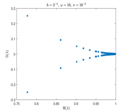
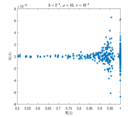
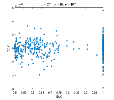
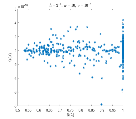
Figure 1: Eigenvalue distribution of $\mathbf{R}_{EPRESB}^{-1}\mathbf{B}$ for $h=2^{-4}$ and $\omega=10$ for $\nu=10^{-k}$, $k=2,4,6,8$.

Table 1: Number of iterations of the methods along with the elapsed CPU time (in parenthesis) for $h=2^{-7}$ and different values of $\nu$ and $\omega$.

	$\nu\setminus\omega$	$10^{-2}$	$10^{-1}$	$1$	$10^{1}$	$10^{2}$
No Prec.	$10^{-2}$	${\dagger}$	${\dagger}$	${\dagger}$	${\dagger}$	${\dagger}$
	$10^{-4}$	${\dagger}$	${\dagger}$	${\dagger}$	${\dagger}$	${\dagger}$
	$10^{-6}$	1303(14.79)	1303(14.76)	1303(14.76)	1303(14.69)	1303(14.74)
	$10^{-8}$	146(1.84)	146(1.87)	146(1.89)	146(1.91)	146(1.86)
$\mathbf{R}_{EPRESB}$	$10^{-2}$	9(0.36)	9(0.35)	9(0.37)	10 (0.40)	24(0.79)
	$10^{-4}$	12(0.45)	12(0.44)	12(0.44)	12(0.44)	18(0.63)
	$10^{-6}$	12(0.44)	12(0.45)	12(0.44)	12(0.43)	12(0.46)
	$10^{-8}$	11(0.40)	11(0.41)	11(0.43)	11(0.42)	11(0.44)
$\mathbf{P}_{BD}$	$10^{-2}$	20(0.58)	20(0.61)	20(0.67)	22(0.67)	26(0.74)
	$10^{-4}$	56(1.45)	56(1.44)	56(1.49)	58(1.56)	48(1.28)
	$10^{-6}$	61(1.61)	61(1.64)	61(1.61)	61(1.61)	62(1.63)
	$10^{-8}$	54(1.41)	54(1.36)	54(1.41)	54(1.46)	54(1.42)
$\mathbf{P}_{BAS}$	$10^{-2}$	16(0.48)	16(0.48)	16(0.50)	18(0.52)	54(1.43)
	$10^{-4}$	22(0.66)	22(0.68)	22(0.67)	22(0.67)	50(1.36)
	$10^{-6}$	22(0.68)	22(0.65)	22(0.68)	22(0.68)	26(0.73)
	$10^{-8}$	22(0.65)	22(0.67)	22(0.67)	22(0.66)	22(0.66)

Table 2: Number of iterations of the methods along with the elapsed CPU time (in parenthesis) for $h=2^{-8}$ and different values of $\nu$ and $\omega$.

	$\nu\setminus\omega$	$10^{-2}$	$10^{-1}$	$1$	$10^{1}$	$10^{2}$
No Prec.	$10^{-2}$	${\dagger}$	${\dagger}$	${\dagger}$	${\dagger}$	${\dagger}$
	$10^{-4}$	${\dagger}$	${\dagger}$	${\dagger}$	${\dagger}$	${\dagger}$
	$10^{-6}$	${\dagger}$	${\dagger}$	${\dagger}$	${\dagger}$	${\dagger}$
	$10^{-8}$	523(26.15)	523(25.77)	523(25.70)	523(25.86)	523(25.58)
$\mathbf{R}_{EPRESB}$	$10^{-2}$	9(1.30)	9(1.30)	9(1.32)	10 (1.39)	24(3.12)
	$10^{-4}$	12(1.62)	12(1.62)	12(1.62)	12(1.66)	18(2.41)
	$10^{-6}$	12(1.63)	12(1.64)	12(1.62)	12(1.63)	12(1.67)
	$10^{-8}$	11(1.51)	11(1.49)	11(1.54)	11(1.50)	11(1.53)
$\mathbf{P}_{BD}$	$10^{-2}$	20(2.57)	20(2.58)	20(2.57)	22(2.84)	26(3.09)
	$10^{-4}$	56(6.32)	56(6.39)	56(6.41)	58(6.67)	49(5.63)
	$10^{-6}$	62(7.16)	62(7.18)	62(7.12)	62(7.19)	63(7.18)
	$10^{-8}$	57(7.10)	57(6.50)	57(6.56)	57(6.62)	57(6.51)
$\mathbf{P}_{BAS}$	$10^{-2}$	16(2.03)	16(2.05)	16(2.05)	18(2.31)	54(6.26)
	$10^{-4}$	22(2.83)	22(2.84)	22(2.83)	22(2.83)	50(5.75)
	$10^{-6}$	22(2.90)	22(2.83)	22(2.84)	22(2.83)	26(3.17)
	$10^{-8}$	22(2.98)	22(2.82)	22(2.84)	22(2.84)	22(2.85)

Table 3: Number of iterations of the methods along with the elapsed CPU time (in parenthesis) for $h=2^{-9}$ and different values of $\nu$ and $\omega$.

	$\nu\setminus\omega$	$10^{-2}$	$10^{-1}$	$1$	$10^{1}$	$10^{2}$
No Prec.	$10^{-2}$	${\dagger}$	${\dagger}$	${\dagger}$	${\dagger}$	${\dagger}$
	$10^{-4}$	${\dagger}$	${\dagger}$	${\dagger}$	${\dagger}$	${\dagger}$
	$10^{-6}$	${\dagger}$	${\dagger}$	${\dagger}$	${\dagger}$	${\dagger}$
	$10^{-6}$	${\dagger}$	${\dagger}$	${\dagger}$	${\dagger}$	${\dagger}$
$\mathbf{R}_{EPRESB}$	$10^{-2}$	9(6.33)	9(6.51)	9(6.38)	10 (6.39)	24(15.73)
	$10^{-4}$	12(8.09)	12(8.15)	12(8.10)	12(8.20)	18(12.07)
	$10^{-6}$	12(8.14)	12(8.18)	12(8.12)	12(8.12)	12(8.14)
	$10^{-8}$	11(7.54)	11(7.49)	11(7.56)	11(7.48)	11(7.56)
$\mathbf{P}_{BD}$	$10^{-2}$	20(13.43)	20(13.36)	20(13.32)	22(14.63)	26(16.39)
	$10^{-4}$	56(33.90)	56(33.78)	56(33.94)	58(35.37)	49(29.46)
	$10^{-6}$	62(38.07)	62(37.55)	62(37.60)	62(37.75)	63(38.02)
	$10^{-8}$	59(35.88)	59(36.29)	59(35.74)	59(35.77)	59(35.48)
$\mathbf{P}_{BAS}$	$10^{-2}$	16(10.68)	16(10.69)	16(10.71)	18(12.05)	54(32.83)
	$10^{-4}$	22(14.83)	22(14.79)	22(14.87)	22(14.72)	50(30.14)
	$10^{-6}$	22(15.18)	22(14.73)	22(14.85)	22(14.87)	26(16.52)
	$10^{-8}$	22(14.73)	22(14.85)	22(14.77)	22(14.85)	22(14.75)

5 Conclusion

We have extended the PRESB preconditioner to a class of non-Hermitian two-by-two complex system of linear equations. Spectral analysis of the preconditioned matrix has been analyzed. We utilized the proposed preconditioner to the systems arising from finite element discretization of PDE-constrained optimization problems. Numerical results show that the proposed preconditioner is efficient and in comparison to two well-known precoditioners is more efficient.

Confict of interest

The authors declare that there is no conflict of interest.

References

- 1 S.R. Arridge, Optical tomography in medical imaging, Inverse Problems 15 (1999) 41–93.
- 2 O. Axelsson, S. Farouq, and M. Neytcheva, Comparison of preconditioned Krylov subspace iteration methods for PDE-constrained optimization problems. Poisson and convection-diffusion control, Numer. Algorithms, 73 (2016) 631–663.
- 3 O. Axelsson, S. Farouq, M. Neytcheva, Comparison of preconditioned Krylov subspace iteration methods for PDE-constrained optimization problems. Stokes Control, Numer. Algorithms 74 (2017) 19–37.
- 4 O. Axelsson, S. Farouq, M. Neytcheva, A preconditioner for optimal control problems constrained by Stokes equation with a time-harmonic control, J. Comput. Appl. Math. 310 (2017) 5–18.
- 5 O. Axelsson, D.K. Salkuyeh, A new version of a preconditioning method for certain two-by-two block matrices with square blocks, BIT Numer. Math. 59 (2019) 321–342.
- 6 O. Axelsson, D. Luk, Preconditioning methods for eddy-current optimally controlled time-harmonic electromagnetic problems, J. Numer. Math. 27 (2019) 1-21.
- 7 O. Axelsson, J. Karátson, Superior properties of the PRESB preconditioner for operators on two-by-two block form with square blocks, Numer. Math. 146 (2020) 335–368.
- 8 Z.-Z. Bai, G.H. Golub, M.K. Ng, Hermitian and skew-Hermitian splitting methods for non-Hermitian positive definite linear systems, SIAM. J. Matrix Anal. Appl. 24 (2003) 603–626.
- 9 Z.-Z. Bai, M. Benzi, F. Chen, Modified HSS iteration methods for a class of complex symmetric linear systems, Computing 87 (2010) 93–111.
- 10 Z.-Z. Bai, M. Benzi, F. Chen, On preconditioned MHSS iteration methods for complex symmetric linear systems, Numer. Algorithms 56 (2011) 297–317.
- 11 D. Bertaccini, Efficient solvers for sequences of complex symmetric linear system, Electron. Trans. Numer. Anal. 18 (2004) 49–64.
- 12 H. Elman, D. Silvester, A.J. Wathen, Finite Elements and Fast Iterative Solvers with Applications in Incompressible Fluid Dynamics, Oxford University Press, 2005.
- 13 A. Feriani, F. Perotti, V. Simoncini, Iterative system solvers for the frequency analysis of linear mechanical systems, Comput. Methods Appl. Mech. Engrg. 190 (2000) 1719–1739.
- 14 A. Frommer, T. Lippert, B. Medeke, K. Schilling, Numerical challenges in lattice quantum chromodynamics, Lecture notes in computational science and engineering 15 (2000) 1719–1739.
- 15 D. Hezari, V. Edalatpour, D.K. Salkuyeh, Preconditioned GSOR iterative method for a class of complex symmetric system of linear equations, Numer. Linear Algebra Appl. 22 (4) 761–776.
- 16 D. Hezari, D.K. Salkuyeh, V. Edalatpour, A new iterative method for solving a class of complex symmetric system of linear equations, Numer. Algorithms 73 (2016) 927–955
- 17 W. Krendl, V. Simoncini, W. Zulehner, Stability estimates and structural spectral properties of saddle point problems, Numer. Math. 124 (2013), 183–213.
- 18 Z.-Z. Liang, O. Axelsson, M. Neytcheva, A robust structured preconditioner for time-harmonic parabolic optimal control problems, Numer. Algorithms 79 (2018) 575–596.
- 19 G. Moro, J.H. Freed, Calculation of ESR spectra and related Fokker-Planck forms by the use of the Lanczos algorithm, J. Chem. Phys. 74 (1981) 3757–3773.
- 20 B. Poirier, Effecient preconditioning scheme for block partitioned matrices with structured sparsity, Numer. Linear Algebra Appl. 7 (2000) 715–726.
- 21 T. Rees, H.S. Dollar, A.J. Wathen, Optimal solvers for PDE-constrained optimization, SIAM J. Sci. Comput. 32 (2010) 271–298.
- 22 Y. Saad, Iterative Methods for Sparse Linear Systems, PWS Press, New York, 1995.
- 23 Y. Saad, M.H Schultz, GMRES: a generalized minimal residual algorithm for solving nonsymmetric linear systems, SIAM J. Sci. Stat. Comput., 7 (1986), 856–869.
- 24 D.K. Salkuyeh, D. Hezari, V. Edalatpour, Generalized successive overrelaxation iterative method for a class of complex symmetric linear system of equations, Int. J. Comput. Math. 92 (2015) 802–815.
- 25 D.K. Salkuyeh, Two-step scale-splitting method for solving complex symmetric system of linear equations, arXiv:1705.02468.
- 26 D.K. Salkuyeh, T.S. Siahkolaei, Two-parameter TSCSP method for solving complex symmetric system of linear equations, Calcolo 55 (2018) 1–22.
- 27 D. Schmitt, B. Steffen, T. Weiland, 2D and 3D computations of lossy eigenvalue problems, IEEE Trans. Magn. 30 (1994) 3578-3581.
- 28 T. Wang, Q.-Q. Zheng, L.-Z. Lu, A new iteration method for a class of complex symmetric linear systems. J. Comput. Appl. Math. 325 (2017) 188–197.
- 29 M.-L. Zeng, Respectively scaled splitting iteration method for a class of block 4-by-4 linear systems from eddy current electromagnetic problems, Japan J. Indust. Appl. Math. 38 (2021) 489–501.
- 30 Z. Zheng, G.-F. Zhang, M.-Z. Zhu, A block alternating splitting iteration method for a class of block two-by-two complex linear systems, J. Comput. Appl. Math. 288 (2015) 203–214.