How to Make the Gradients Small Privately:
Improved Rates for Differentially Private Non-Convex Optimization

Abstract

We provide a simple and flexible framework for designing differentially private algorithms to find approximate stationary points of non-convex loss functions. Our framework is based on using a private approximate risk minimizer to “warm start” another private algorithm for finding stationary points. We use this framework to obtain improved, and sometimes optimal, rates for several classes of non-convex loss functions. First, we obtain improved rates for finding stationary points of smooth non-convex empirical loss functions. Second, we specialize to quasar-convex functions, which generalize star-convex functions and arise in learning dynamical systems and training some neural nets. We achieve the optimal rate for this class. Third, we give an optimal algorithm for finding stationary points of functions satisfying the Kurdyka-Łojasiewicz (KL) condition. For example, over-parameterized neural networks often satisfy this condition. Fourth, we provide new state-of-the-art rates for stationary points of non-convex population loss functions. Fifth, we obtain improved rates for non-convex generalized linear models. A modification of our algorithm achieves nearly the same rates for second-order stationary points of functions with Lipschitz Hessian, improving over the previous state-of-the-art for each of the above problems.

1 Introduction

The increasing prevalence of machine learning (ML) systems, such as large language models (LLMs), in societal contexts has led to growing concerns about the privacy of these models. Extensive research has demonstrated that ML models can leak the training data of individuals, violating their privacy (Shokri et al., 2017; Carlini et al., 2021). For instance, individual training examples were extracted from GPT-2 using only black-box queries (Carlini et al., 2021). Differential privacy (DP) (Dwork et al., 2006) provides a rigorous guarantee that training data cannot be leaked. Informally, it guarantees that an adversary cannot learn much more about an individual piece of training data than they could have learned had that piece never been collected.

Differentially private optimization has been studied extensively over the last 10–15 years (Bassily et al., 2014, 2019; Feldman et al., 2020; Asi et al., 2021; Lowy and Razaviyayn, 2023b). Despite this large body of work, certain fundamental and practically important problems remain open. In particular, for minimizing non-convex functions, which is ubiquitous in ML applications, we have a poor understanding of the optimal rates achievable under DP.

In this work, we measure the performance of an algorithm for optimizing a non-convex function $g$ by its ability to find an $\alpha$-stationary point, meaning a point $w$ such that

$$\|\nabla g(w)\|\leq\alpha.$$

We want to understand the smallest $\alpha$ achievable. There are several reasons to study stationary points. First, finding approximate global minima is intractable for general non-convex functions (Murty and Kabadi, 1985), but finding an approximate stationary point is tractable. Second, there are many important non-convex problems for which all stationary (or second-order stationary) points are global minima (e.g. phase retrieval (Sun et al., 2018), matrix completion (Ge et al., 2016), and training certain classes of neural networks (Liu et al., 2022)). Third, even for problems where it is tractable to find approximate global minima, the stationarity gap may be a better measure of quality than the excess risk (Nesterov, 2012; Allen-Zhu, 2018).

Stationary Points of Empirical Loss Functions.

A fundamental open problem in DP optimization is determining the sample complexity of finding stationary points of non-convex empirical loss functions

$$\widehat{F}_{X}(w):=\frac{1}{n}\sum_{i=1}^{n}f(w,x_{i}),$$

where $X=(x_{1},\ldots,x_{n})$ denotes a fixed data set. For convex loss functions, the minimax optimal complexity of DP empirical risk minimization is $\widehat{F}_{X}(w)-\min_{w^{\prime}}\widehat{F}_{X}(w^{\prime})=\tilde{\Theta}(\sqrt{d\ln(1/\delta)}/\varepsilon n)$ (Bun et al., 2014; Bassily et al., 2014; Steinke and Ullman, 2016). Here $d$ is the dimension of the parameter space and $\varepsilon,\delta$ are the privacy parameters. However, the algorithm of Bassily et al. (2014) was suboptimal in terms of finding DP stationary points. This gap was recently closed by (Arora et al., 2023), who showed that the optimal rate for stationary points of convex $\widehat{F}_{X}$ is $\mathbb{E}\|\nabla\widehat{F}_{X}(w)\|=\widetilde{\Theta}(\sqrt{d\ln(1/\delta)}/\varepsilon n)$. For non-convex $\widehat{F}_{X}$, the best known rate prior to 2022 was $O((\sqrt{d\ln(1/\delta)}/\varepsilon n)^{1/2})$ (Zhang et al., 2017; Wang et al., 2017, 2019). In the last two years, a pair of papers made progress and obtained improved rates of $\widetilde{O}((\sqrt{d\ln(1/\delta)}/\varepsilon n)^{2/3})$ (Arora et al., 2023; Tran and Cutkosky, 2022). Arora et al. (2023) gave a detailed discussion of the challenges of further improving beyond the $\widetilde{O}((\sqrt{d\ln(1/\delta)}/\varepsilon n)^{2/3})$ rate. Thus, a natural question is:

Question 1. Can we improve the $\widetilde{O}((\sqrt{d\ln(1/\delta)}/\varepsilon n)^{2/3}$ rate for DP stationary points of smooth non-convex empirical loss functions?

Contribution 1. We answer Question 1 affirmatively, giving a novel DP algorithm that finds a $\widetilde{O}((\sqrt{d\ln(1/\delta)}/\varepsilon n)d^{1/6})$-stationary point. This rate improves over the prior state-of-the-art whenever $d<n\varepsilon$.

Contribution 2. We provide algorithms that achieve the optimal rate $\widetilde{O}((\sqrt{d\ln(1/\delta)}/\varepsilon n))$ for two subclasses of non-convex loss functions: quasar-convex functions (Hinder et al., 2020), which generalize star-convex functions (Nesterov and Polyak, 2006), and Kurdyka-Łojasiewicz (KL) functions (Kurdyka, 1998), which generalize Polyak-Łojasiewicz (PL) functions (Polyak, 1963). Quasar-convex functions arise in learning dynamical systems and training recurrent neural nets (Hardt et al., 2018; Hinder et al., 2020). Also, the loss functions of some neural networks may be quasar-convex in large neighborhoods of the minimizers (Kleinberg et al., 2018; Zhou et al., 2019). On the other hand, the KL condition is satisfied by overparameterized neural networks in many scenarios (Bassily et al., 2018; Liu et al., 2020; Scaman et al., 2022). This is the first time that the optimal rate has been achieved without assuming convexity. To the best of our knowledge, no other DP algorithm in the literature would be able to get the optimal rate for either of these function classes.

Second-Order Stationary Points.

Recently, Wang and Xu (2021); Gao and Wright (2023); Liu et al. (2023) provided DP algorithms for finding $\alpha$-second-order stationary points (SOSP) of functions $g$ with $\rho$-Lipschitz Hessian. A point $w$ is an $\alpha$-SOSP of $g$ if $w$ is an $\alpha$-FOSP and

$$\nabla^{2}g(w)\succeq-\sqrt{\alpha\rho}~{}\mathbf{I}_{d}.$$

The state-of-the-art rate for $\alpha$-SOSPs of empirical loss functions is due to Liu et al. (2023): $\alpha=\widetilde{O}((\sqrt{d\ln(1/\delta)}/\varepsilon n)^{2/3})$, which matches the state-of-the-art rate for FOSPs (Arora et al., 2023; Tran and Cutkosky, 2022).

Contribution 3. Our framework readily extends to SOSPs and achieves an improved $\widetilde{O}((\sqrt{d\ln(1/\delta)}/\varepsilon n)d^{1/6})$ second-order-stationarity guarantee.

Stationary Points of Population Loss Functions.

Moving beyond empirical loss functions, we also consider finding stationary points of population loss functions

$$F(w):=\mathbb{E}_{x\sim\mathcal{P}}[f(w,x)],$$

where $\mathcal{P}$ is some unknown data distribution and we are given $n$ i.i.d. samples $X\sim\mathcal{P}^{n}$. The prior state-of-the-art rate for finding SOSPs of $F$ is $\widetilde{O}(1/n^{1/3}+(\sqrt{d}/\varepsilon n)^{3/7})$ (Liu et al., 2023).

Contribution 4. We give an algorithm that improves over the state-of-the-art rate for SOSPs of the population loss in the regime $d<n\varepsilon$. When $d=\Theta(1)=\varepsilon$, our algorithm is optimal and matches the non-private lower bound $\Omega(1/\sqrt{n})$.

We also specialize to (non-convex) generalized linear models (GLMs), which have been studied privately in (Song et al., 2021; Bassily et al., 2021a; Arora et al., 2022, 2023; Shen et al., 2023). GLMs arise, for instance, in robust regression (Amid et al., 2019) or when fine-tuning the last layers of a neural network. Thus, this problem has applications in privately fine-tuning LLMs (Yu et al., 2021; Li et al., 2021). Denoting the rank of the design matrix $X$ by $r\leq\min(d,n)$, the previous state-of-the-art rate for finding FOSPs of GLMs was $O(1/\sqrt{n}+\min\{(\sqrt{r}/\varepsilon n)^{2/3},1/(\varepsilon n)^{2/5}\})$ (Arora et al., 2023).

Contribution 5. We provide improved rates of finding first- and second-order stationary points of the population loss of GLMs. Our algorithm finds a $\widetilde{O}(1/\sqrt{n}+\min\{(\sqrt{r}/\varepsilon n)r^{1/6},1/(\varepsilon n)^{2/7}\}$-stationary point, which is better than Arora et al. (2023) when $r<n\varepsilon$.

A summary of our main results is given in Table 1.

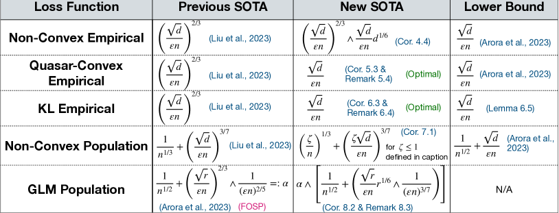
Figure 1: Summary of results for second-order stationary points (SOSP). All bounds should be read as $\min(1,...)$. SOTA = state-of-the-art. $\zeta:=1\wedge\left(\frac{d}{\varepsilon n}+\sqrt{\frac{d}{n}}\right)$. $r:=\mbox{rank}(X)$. We omit logarithms, Lipschitz and smoothness paramaters. The GLM algorithm of (Arora et al., 2023) only finds FOSP, not SOSP.

1.1 Our Approach

Our algorithmic approach is inspired by Nesterov, who proposed the following method for finding stationary points in non-private convex optimization: first run $T$ steps of accelerated gradient descent (AGD) to obtain $w_{0}$, and then run $T$ steps of gradient descent (GD) initialized at $w_{0}$ (Nesterov, 2012). Nesterov’s approach provided improved stationary guarantees for convex loss functions, compared to running either AGD or GD alone.

We generalize and extend Nesterov’s approach to private non-convex optimization. We first observe that there is nothing special about AGD or GD that makes his approach work. As we will see, one can obtain improved (DP) stationarity guarantees by running algorithm $\mathcal{B}$ after algorithm $\mathcal{A}$, provided that: (a) $\mathcal{A}$ moves us in the direction of a global minimizer, and (b) the stationarity guarantee of $\mathcal{B}$ benefits from a small initial suboptimality gap. Intuitively, the algorithm $\mathcal{A}$ functions as a “warm start” that gets us a bit closer to a global minimizer, which allows $\mathcal{B}$ to converge faster.

1.2 Roadmap

Section 2 contains relevant definitions, notations, and assumptions. In Section 3, we describe our general algorithmic framework and provide privacy and stationarity guarantees. The remaining sections contain applications of our algorithmic framework to non-convex empirical losses (Section 4), quasar-convex losses (Section 5), KL losses (Section 6), population losses (Section 7), and GLMs (Section 8).

2 Preliminaries

We consider loss functions $f:\mathbb{R}^{d}\times\mathcal{X}\to\mathbb{R}$, where $\mathcal{X}$ is a data universe. For a data set $X\in\mathcal{X}^{n}$, let $\widehat{F}_{X}(w):=\frac{1}{n}\sum_{i=1}^{n}f(w,x_{i})$ denote the empirical loss function. Let $F(w):=\mathbb{E}_{x\sim P}[f(w,x)]$ denote the population loss function with respect to some unknown data distribution $P$.

Assumptions and Notation.

Definition 2.1 (Lipschitz continuity).

Function $g:\mathbb{R}^{d}\to\mathbb{R}$ is $L$-Lipschitz if $|g(w)-g(w^{\prime})|\leq L\|w-w^{\prime}\|_{2}$ for all $w,w^{\prime}\in\mathbb{R}^{d}$.

Definition 2.2 (Smoothness).

Function $g:\mathbb{R}^{d}\to\mathbb{R}$ is $\beta$-smooth if $g$ is differentiable and has $\beta$-Lipschitz gradient: $\|\nabla g(w)-\nabla g(w^{\prime})\|_{2}\leq\beta\|w-w^{\prime}\|_{2}$.

We assume the following throughout:

Assumption 2.3.

1. $f(\cdot,x)$ is $L$-Lipschitz for all $x\in\mathcal{X}$.

2. $f(\cdot,x)$ is $\beta$-smooth for all $x\in\mathcal{X}$.

3. $\widehat{F}_{X}^{*}:=\inf_{w}\widehat{F}_{X}(w)>-\infty$ for empirical loss optimization, or $F^{*}:=\inf_{w}F(w)>-\infty$ for population.

Definition 2.4 (Stationary Points).

Let $\alpha\geq 0$. We say $w$ is an $\alpha$-first-order-stationary point (FOSP) of function $g$ if $\|\nabla g(w)\|\leq\alpha$. If the Hessian $\nabla^{2}g$ is $\rho$-Lipschitz, then $w$ is an $\alpha$-second-order-stationary point (SOSP) of $g$ if $\|\nabla g(w)\|\leq\alpha$ and $\nabla^{2}g(w)\succeq-\sqrt{\rho\alpha}~{}\mathbf{I}_{d}$.

For functions $a=a(\theta)$ and $b=b(\phi)$ of input parameter vectors $\theta$ and $\phi$, we write $a\lesssim b$ if there is an absolute constant $C>0$ such that $a\leq Cb$ for all values of input parameter vectors $\theta$ and $\phi$. We use $\tilde{O}$ to hide logarithmic factors. Denote $a\wedge b=\min(a,b)$.

Differential Privacy.

Definition 2.5 (Differential Privacy (Dwork et al., 2006)).

Let $\varepsilon\geq 0,~{}\delta\in[0,1).$ A randomized algorithm $\mathcal{A}:\mathcal{X}^{n}\to\mathcal{W}$ is $(\varepsilon,\delta)$-differentially private (DP) if for all pairs of data sets $X,X^{\prime}\in\mathcal{X}^{n}$ differing in one sample and all measurable subsets $S\subseteq\mathcal{W}$, we have

$$\mathbb{P}(\mathcal{A}(X)\in S)\leq e^{\varepsilon}\mathbb{P}(\mathcal{A}(X^{\prime})\in S)+\delta.$$

An important fact about DP is that it composes nicely:

Lemma 2.6 (Basic Composition).

If $\mathcal{A}$ is $(\varepsilon_{1},\delta_{1})$-DP and $\mathcal{B}$ is $(\varepsilon_{2},\delta_{2})$-DP, then $\mathcal{B}\circ\mathcal{A}$ is $(\varepsilon_{1}+\varepsilon_{2},\delta_{1}+\delta_{2})$-DP.

For a proof, see e.g., (Dwork and Roth, 2014). There is also tighter version of the composition result—the advanced composition theorem—which we re-state in Appendix B.

3 Our Warm-Start Algorithmic Framework

For ease of presentation, we will first present a concrete instantiation of our algorithmic framework for ERM, built upon the DP-SPIDER algorithm of Arora et al. (2023), which is described in Algorithm 1.

Algorithm 1 DP-SPIDER (Arora et al., 2023)

  Input: Data $X\in\mathcal{X}^{n}$, loss function $f(w,x)$, $(\varepsilon,\delta)$, initialization $w_{0}$, stepsize $\eta$, iteration number $T$, phase length $q$, noise variances $\sigma_{1}^{2},\sigma_{2}^{2},\hat{\sigma}_{2}^{2}$, batch sizes $b_{1},b_{2}$.

  for $t=0,\ldots,T-1$ do

     if $q|t$ then

        Sample batch $S_{t}$ of size $b_{1}$

        Sample $g_{t}\sim\mathcal{N}(0,\sigma_{1}^{2}\mathbf{I}_{d})$

        $\nabla_{t}=\frac{1}{b_{1}}\sum_{x\in S_{t}}\nabla f(w_{t},x)+g_{t}$

     else

        Sample batch $S_{t}$ of size $b_{2}$

        Sample $h_{t}\sim\mathcal{N}(0,\min\{\sigma_{2}^{2}\|w_{t}-w_{t-1}\|^{2},\hat{\sigma_{2}}^{2}\}\mathbf{I}_{d})$

        $\Delta_{t}=\frac{1}{b_{2}}\sum_{x\in S_{t}}[\nabla f(w_{t},x)-\nabla f(w_{t-1},x)]+h_{t}$

        $\nabla_{t}=\nabla_{t-1}+\Delta_{t}$

     end if

     $w_{t+1}=w_{t}-\eta\nabla_{t}$

  end for

  Return: $\hat{w}\sim\textbf{Unif}(w_{1},\ldots,w_{T})$.

For initialization $w_{0}\in\mathbb{R}^{d}$, denote the suboptimality gap by

$$\hat{\Delta}_{w_{0}}:=\widehat{F}_{X}(w_{0})-\widehat{F}_{X}^{*}.$$

We recall the guarantees of DP-SPIDER below:

Lemma 3.1.

(Arora et al., 2023) There exist algorithmic parameters such that Algorithm 1 is $(\varepsilon/2,\delta/2)$-DP and returns $\hat{w}$ satisfying

$$\mathbb{E}\|\nabla\widehat{F}_{X}(\hat{w})\|\lesssim\left(\frac{\sqrt{\hat{\Delta}_{w_{0}}L\beta}\sqrt{d\ln(1/\delta)}}{\varepsilon n}\right)^{2/3}+\frac{L\sqrt{d\ln(1/\delta)}}{\varepsilon n}.$$ (1)

Typically, the first term on the right-hand-side of 1 is dominant.

Our algorithm is based on a simple observation: the stationarity guarantee in Lemma 3.1 depends on the initial suboptimality gap $\hat{\Delta}_{w_{0}}$. Therefore, if we can privately find a good “warm start” point $w_{0}$ such that $\widehat{F}_{X}(w_{0})-\widehat{F}_{X}^{*}$ is small with high probability, then we can run DP-SPIDER initialized at $w_{0}$ to improve over the $O((\sqrt{d}/\varepsilon n)^{2/3})$ guarantee of DP-SPIDER. More generally, we can apply any DP stationary point finder $\mathcal{B}$ with initialization $w_{0}$ after warm starting. Pseudocode for our general meta-algorithm is given in Algorithm 2.

Algorithm 2 Warm-Start Meta-Algorithm for ERM

  Input: Data $X\in\mathcal{X}^{n}$, loss function $f(w,x)$, privacy parameters $(\varepsilon,\delta)$, warm-start DP-ERM algorithm $\mathcal{A}$, DP-ERM stationary point finder $\mathcal{B}$.

  Run $(\varepsilon/2,\delta/2)$-DP $\mathcal{A}$ on $\widehat{F}_{X}(\cdot)$ to obtain $w_{0}$.

  Run $\mathcal{B}$ on $\widehat{F}_{X}(\cdot)$ with initialization $w_{0}$ and privacy parameters $(\varepsilon/2,\delta/2)$ to obtain $w_{\text{priv}}$.

  Return: $w_{\text{priv}}$.

We have the following guarantee for Algorithm 2 instantiated with $\mathcal{B}=$ Algorithm 1.

Theorem 3.2 (First-Order Stationary Points for ERM: Meta-Algorithm).

Let $\zeta\leq\sqrt{d}/\varepsilon n$. Suppose $\mathcal{A}$ is $(\varepsilon/2,\delta/2)$-DP and $\widehat{F}_{X}(\mathcal{A}(X))-\widehat{F}_{X}^{*}\leq\psi$ with probability $\geq 1-\zeta$. Then, Algorithm 2 with $\mathcal{B}$ as DP-SPIDER is $(\varepsilon,\delta)$-DP and returns $w_{\text{priv}}$ with

$$\mathbb{E}\|\nabla\widehat{F}_{X}(w_{\text{priv}})\|\lesssim\frac{L\sqrt{d\ln(1/\delta)}}{\varepsilon n}+L^{1/3}\beta^{1/3}\psi^{1/3}\left(\frac{\sqrt{d\ln(1/\delta)}}{\varepsilon n}\right)^{2/3}.$$

Proof.

Privacy follows from Lemma 2.6, since $\mathcal{A}$ and DP-SPIDER are both $(\varepsilon/2,\delta/2)$-DP.

For the stationarity guarantee, let $E$ be the high-probability good event that $\widehat{F}_{X}(\mathcal{A}(X))-\widehat{F}_{X}^{*}\leq\psi$. Then, by Lemma 3.1, we have

$$\mathbb{E}\left[\|\nabla\widehat{F}_{X}(w_{\text{priv}})\||E\right] \lesssim\left(\frac{\sqrt{\psi L\beta}\sqrt{d\ln(1/\delta)}}{\varepsilon n}\right)^{2/3}$$

$$\;\;\;\;+\frac{L\sqrt{d\ln(1/\delta)}}{\varepsilon n}.$$

On the other hand, if $E$ does not hold, then we still have $\|\nabla\widehat{F}_{X}(w_{\text{priv}})\|\leq L$ by Lipschitz continuity. Thus, taking total expectation yields

$$\mathbb{E}\|\nabla\widehat{F}_{X}(w_{\text{priv}})\| \leq\mathbb{E}\left[\|\nabla\widehat{F}_{X}(w_{\text{priv}})\||E\right](1-\zeta)+L\zeta$$

$$\lesssim\left(\frac{\sqrt{\psi L\beta}\sqrt{d\ln(1/\delta)}}{\varepsilon n}\right)^{2/3}$$

$$\;\;\;\;+\frac{L\sqrt{d\ln(1/\delta)}}{\varepsilon n}+L\zeta.$$

Since $\zeta\leq\sqrt{d}/\varepsilon n$, the result follows. ∎

Note that if we instantiate Algorithm 2 with any DP $\mathcal{B}$, we can obtain an algorithm that improves over the stationarity guarantee of $\mathcal{B}$ as long as the stationarity guarantee of $\mathcal{B}$ scales with the initial suboptimality gap $\hat{\Delta}_{w_{0}}$. In particular, our framework allows for improved rates of finding second-order stationarity points, by choosing $\mathcal{B}$ as the DP SOSP finder of Liu et al. (2023) (which is built on DP-SPIDER). We recall the privacy and utility guarantees of this algorithm—which we refer to as DP-SPIDER-SOSP—below in Lemma 3.3. For convenience, denote

$$\alpha :=\left(\frac{\sqrt{\hat{\Delta}_{w_{0}}L\beta}\sqrt{d\ln(1/\delta)}}{\varepsilon n}\right)^{2/3}+\frac{L\sqrt{d\ln(1/\delta)}}{\varepsilon n}+\frac{\beta}{n\sqrt{\rho}}\left(\frac{\sqrt{\hat{\Delta}_{w_{0}}L\beta}\sqrt{d\ln(1/\delta)}}{\varepsilon n}\right)^{1/3}.$$

Lemma 3.3.

(Liu et al., 2023) Assume that $f(\cdot,x)$ has $\rho$-Lipschitz Hessian $\nabla^{2}f(\cdot,x)$. Then, there is an $(\varepsilon/2,\delta/2)$-DP Algorithm (DP-SPIDER-SOSP), that returns $\hat{w}$ such that with probability $\geq 1-\zeta$, $\hat{w}$ is a $\widetilde{O}(\alpha)$-SOSP of $\widehat{F}_{X}$.

Next, we provide the guarantee of Algorithm 2 instantiated with $\mathcal{B}$ as DP-SPIDER-SOSP:

Theorem 3.4 (Second-order Stationary Points for ERM: Meta-Algorithm).

Suppose $\mathcal{A}$ is $(\varepsilon/2,\delta/2)$-DP and $\widehat{F}_{X}(\mathcal{A}(X))-\widehat{F}_{X}^{*}\leq\psi$ with probability $\geq 1-\zeta$. Then, Algorithm 2 with $\mathcal{B}$ as DP-SPIDER-SOSP is $(\varepsilon,\delta)$-DP, and with probability $\geq 1-2\zeta$ has output $w_{\text{priv}}$ satisfying

$$\|\nabla\widehat{F}_{X}(w_{\text{priv}})\| \leq\tilde{\alpha}:=\widetilde{O}\left(\frac{L\sqrt{d\ln(1/\delta)}}{\varepsilon n}+L^{1/3}\beta^{1/3}\psi^{1/3}\left(\frac{\sqrt{d\ln(1/\delta)}}{\varepsilon n}\right)^{2/3}+\frac{\beta^{7/6}L^{1/6}\psi^{1/6}}{n\sqrt{\rho}}\left(\frac{\sqrt{d\ln(1/\delta)}}{\varepsilon n}\right)^{1/3}\right),$$

and

$$\nabla^{2}\widehat{F}_{X}(w_{\text{priv}})\succeq-\sqrt{\rho\tilde{\alpha}}~{}\mathbf{I}_{d}.$$

The proof is similar to the proof of Theorem 3.2, and is deferred to Appendix C.

With Algorithm 2, we have reduced the problem of finding an approximate stationary point $w_{\text{priv}}$ to finding an approximate excess risk minimizer $w_{0}$. The next question is: What should we choose as our warm-start algorithm $\mathcal{A}$? The right answer depends on the function. In the following sections, we consider different classes of non-convex functions and instantiate Algorithm 2 with an appropriate warm-start $\mathcal{A}$ for each class to obtain new state-of-the-art rates.

4 Improved Rates for Stationary Points of Non-Convex Empirical Losses

In this section, we provide improved rates for finding (first-order and second-order) stationary points of smooth non-convex empirical loss functions. For the non-convex loss functions satisfying Assumption 2.3, we propose using the exponential mechanism (McSherry and Talwar, 2007) as our warm-start algorithm $\mathcal{A}$ in Algorithm 2.

We now recall the exponential mechanism. Assume that there is a compact set $\mathcal{W}\subset\mathbb{R}^{d}$ containing an approximate global minimizer $w^{*}$ such that $\widehat{F}_{X}(w^{*})-\widehat{F}_{X}^{*}\leq LD\frac{d}{\varepsilon n}$, and that $\|w-w^{\prime}\|_{2}\leq D$ for all $w,w^{\prime}\in\mathcal{W}$. Note that there exists a finite $D\frac{d}{\varepsilon n}$-net for $\mathcal{W}$, denoted $\widetilde{\mathcal{W}}=\{w_{1},\ldots,w_{N}\}$, with $N:=|\widetilde{\mathcal{W}}|\leq\left(\frac{2D\varepsilon n}{d}\right)^{d}$. In particular, $\min_{i\in[N]}\widehat{F}_{X}(w_{i})-\widehat{F}_{X}^{*}\leq 2LD\frac{d}{\varepsilon n}$.

Definition 4.1 (Exponential Mechanism for ERM).

Given inputs $\widehat{F}_{X},\widetilde{\mathcal{W}}$, the exponential mechanism $\mathcal{A}_{E}$ selects and outputs some $w\in\widetilde{\mathcal{W}}$. The probability that a particular $w$ is selected is proportional to $\exp\left(\frac{-\varepsilon n\widehat{F}_{X}(w)}{4LD}\right)$.

The following lemma specializes (Dwork and Roth, 2014, Theorem 3.11) to our ERM setting:

Lemma 4.2.

The exponential mechanism $\mathcal{A}_{E}$ is $\varepsilon$-DP. Moreover, $\forall t>0$, we have with probability at least $1-\exp(-t)$ that

$$\widehat{F}_{X}(\mathcal{A}_{E})-\widehat{F}_{X}(w^{*}) \leq\frac{4LD}{\varepsilon n}\ln\left(\left(\frac{2\varepsilon n}{d}\right)^{d}+t\right)+2LD\frac{d}{\varepsilon n}.$$

First-Order Stationary Points.

For convenience, denote

$$\gamma:=\frac{L\sqrt{d\ln(1/\delta)}}{\varepsilon n}+\widetilde{O}\left(L^{2/3}\beta^{1/3}D^{1/3}\frac{\sqrt{d\ln(1/\delta)}}{\varepsilon n}d^{1/6}\right).$$

By substituting $\varepsilon/2$ for $\varepsilon$ and then choosing $t=\ln(\varepsilon n/2\sqrt{d})$ in Lemma 4.2, the $\varepsilon/2$-exponential mechanism returns a point $w_{0}$ such that

$$\widehat{F}_{X}(w_{0})-\widehat{F}_{X}^{*}\leq 20LD\frac{d}{\varepsilon n}\ln(\varepsilon n/\sqrt{d})=:\psi$$ (2)

with probability at least $1-2\frac{\sqrt{d}}{\varepsilon n}$. By plugging the above $\psi$ into Theorem 3.2, we obtain:

Corollary 4.3 (First-Order Stationary Points for Non-Convex ERM).

There exist algorithmic parameters such that Algorithm 2 with $\mathcal{A}=\mathcal{A}_{E}$ and $\mathcal{B}=$DP-SPIDER is $(\varepsilon,\delta)$-DP and returns $w_{\text{priv}}$ such that

$$\mathbb{E}\|\nabla\widehat{F}_{X}(w_{\text{priv}})\| \lesssim\gamma.$$

If $L,\beta,D$ are constants, then Corollary 4.3 gives $\mathbb{E}\|\nabla\widehat{F}_{X}(w_{\text{priv}})\|=\widetilde{O}\left(\frac{\sqrt{d\ln(1/\delta)}}{\varepsilon n}d^{1/6}\right)$. This bound is bigger than the lower bound by a factor of $d^{1/6}$ and improves over the previous state-of-the-art $O\left(\frac{\sqrt{d\ln(1/\delta)}}{\varepsilon n}\right)^{2/3}$ whenever $d<n\varepsilon$ (Arora et al., 2023). If $d\geq n\varepsilon$, then one should simply run DP-SPIDER. Combining these two algorithms gives a new state-of-the-art bound for DP stationary points of non-convex empirical loss functions:

$$\mathbb{E}\|\nabla\widehat{F}_{X}(w_{\text{priv}})\|\lesssim\frac{\sqrt{d\ln(1/\delta)}}{\varepsilon n}d^{1/6}\wedge\left(\frac{\sqrt{d\ln(1/\delta)}}{\varepsilon n}\right)^{2/3}.$$

Challenges of Further Rate Improvements.

We believe that it is not possible for Algorithm 2 to achieve a better rate than Corollary 4.3 by choosing $\mathcal{A}$ differently. The exponential mechanism is optimal for non-convex Lipschitz empirical risk minimization (Ganesh et al., 2023). Although the lower bound function in Ganesh et al. (2023) is not $\beta$-smooth, we believe that one can smoothly approximate it (e.g. by piecewise polynomials) to extend the same lower bound to smooth functions. For large enough $\beta$, their lower bound extends to smooth losses by simple convolution smoothing. Thus, a fundamentally different algorithm may be needed to find $O(\sqrt{d\ln(1/\delta)}/\varepsilon n)$-stationary points for general non-convex empirical losses.

Second-Order Stationary Points.

If we assume that $f$ has Lipschitz continuous Hessian, then we can instantiate Algorithm 2 with $\mathcal{B}$ as DP-SPIDER-SOSP to obtain:

Corollary 4.4 (Second-Order Stationary Points for Non-Convex ERM).

Let $\zeta>0$. Suppose $\nabla^{2}f(\cdot,x)$ is $\rho$-Lipschitz $\forall x$. Then, Algorithm 2 with $\mathcal{A}=\mathcal{A}_{E}$ and $\mathcal{B}=$ DP-SPIDER-SOSP is $(\varepsilon,\delta)$-DP and with probability $\geq 1-\zeta$, returns a $\omega$-SOSP, where

$$\omega:=\gamma+\widetilde{O}\left(\frac{L^{1/3}D^{1/6}\beta^{7/6}}{\sqrt{\rho}n}\left(\frac{\sqrt{d\ln(1/\delta)}}{\varepsilon n}\right)^{1/2}d^{1/12}\right),$$

If $L,\beta,D$ and $\rho$ are constants, then Corollary 4.4 implies that Algorithm 2 finds a $\widetilde{O}(d^{1/6}\sqrt{d\ln(1/\delta)}/\varepsilon n)$-second-order stationary point of $\widehat{F}_{X}$. This result improves over the previous state-of-the-art (Liu et al., 2023) when $d<n\varepsilon$.

5 Optimal Rate for Quasar-Convex Losses

In this section, we specialize to quasar-convex loss functions (Hardt et al., 2018; Hinder et al., 2020) and show, for the first time, that it is possible to attain the optimal (up to logs) rate $\widetilde{O}(\sqrt{d\ln(1/\delta)}/\varepsilon n)$ for stationary points, without assuming convexity.

Definition 5.1 (Quasar-convex functions).

Let $q\in(0,1]$ and let $w^{*}$ be a minimizer of differentiable function $g:\mathbb{R}^{d}\to\mathbb{R}$. $g$ is $q$-quasar convex if for all $w\in\mathbb{R}^{d}$, we have

$$g(w^{*})\geq g(w)+\frac{1}{q}\langle\nabla g(w),w^{*}-w\rangle.$$

Quasar-convex functions generalize star-convex functions (Nesterov and Polyak, 2006), which are quasar-convex functions with $q=1$. Smaller values of $q<1$ allow for a greater degree of non-convexity.

Proposition 5.2 shows that returning a uniformly random iterate of DP-SGD (Algorithm 3) attains essentially the same (optimal) rate for quasar-convex ERM as for convex ERM:

Algorithm 3 DP-SGD for Quasar-Convex

1:  Input: Loss function $f$, data $X$, iteration number $T$ noise variance $\sigma^{2}$, step size $\eta$, batch size $b$.

2:  Initialize $w_{1}\in\mathbb{R}^{d}$.

3:  for $t\in\{1,2,\cdots,T\}$ do

4:     Sample batch $S_{t}$ of size $b$ from $X$

5:     Sample $u_{t}\sim\mathcal{N}(0,\sigma^{2}\mathbf{I}_{d})$

6:     $\nabla_{t}=\frac{1}{b}\sum_{x\in S_{t}}\nabla f(w_{t},x)+u_{t}$

7:     $w_{t+1}=w_{t}-\eta\nabla_{t}$.

8:  end for

9:  Output: $\hat{w}\sim\textbf{Unif}(w_{1},\ldots,w_{T})$.

Proposition 5.2.

Let $\widehat{F}_{X}$ be $q$-quasar convex and $\|w_{1}-w^{*}\|\leq D$ for $w^{*}\in\operatorname*{argmin}_{w}\widehat{F}_{X}(w)$. Then, there are algorithmic parameters such that Algorithm 3 is $(\varepsilon,\delta)$-DP, and returns $\hat{w}$ such that

$$\mathbb{E}\widehat{F}_{X}(\hat{w})-\widehat{F}_{X}^{*}\lesssim LD\frac{\sqrt{d\ln(1/\delta)}}{\varepsilon nq}.$$

Further, $\forall~{}\zeta>0$, there is an $(\varepsilon,\delta)$-DP variation of Algorithm 3 that returns $\tilde{w}$ s.t. with probability at least $1-\zeta$,

$$\widehat{F}_{X}(\tilde{w})-\widehat{F}_{X}^{*}=\widetilde{O}\left(LD\frac{\sqrt{d\ln(1/\delta)}}{\varepsilon nq}\right).$$

See Appendix D for a proof. The same proof works for non-smooth quasar-convex losses if we replace gradients by subgradients in Algorithm 3. As a byproduct, our proof yields a novel non-private optimization result: SGD achieves the optimal $O(1/\sqrt{T})$ rate for Lipschitz non-smooth quasar-convex stochastic optimization. To our knowledge, this result was only previously recorded for smooth losses (Gower et al., 2021) or convex losses (Nesterov, 2013).

By combining Proposition 5.2 with Theorem 3.2, we obtain:

Corollary 5.3 (Quasar-Convex ERM).

Let $\widehat{F}_{X}$ be $q$-quasar convex and $\|w_{1}-w^{*}\|\leq D$ for some $w_{1}\in\mathbb{R}^{d},w^{*}\in\operatorname*{argmin}_{w}\widehat{F}_{X}(w)$. Then, there are algorithmic parameters such that Algorithm 2 with $\mathcal{A}=$ Algorithm 3 and $\mathcal{B}=$ DP-SPIDER is $(\varepsilon,\delta)$-DP and returns $w_{\text{priv}}$ such that

$$\mathbb{E}\|\nabla\widehat{F}_{X}(w_{\text{priv}})\| \lesssim L\frac{\sqrt{d\ln(1/\delta)}}{\varepsilon n}+\widetilde{O}\left(L^{2/3}\beta^{1/3}D^{1/3}\frac{\sqrt{d\ln(1/\delta)}}{\varepsilon nq}\right).$$

If $q$ is constant and $\beta D\lesssim L$, then this rate is optimal up to a logarithmic factor, since it matches the convex (hence quasar-convex) lower bound of Arora et al. (2023).

Remark 5.4.

One can obtain a second-order stationary point with essentially the same (near-optimal) rate by appealing to Theorem 3.4 instead of Theorem 3.2.

6 Optimal Rates for KL* Empirical Losses

In this section, we derive optimal rates (up to logarithms) for functions satisfying the Kurdyka-Łojasiewicz* (KL*) condition (Kurdyka, 1998):

Definition 6.1.

Let $\gamma,k>0$. Function $g:\mathbb{R}^{d}\to\mathbb{R}$ satisfies the $(\gamma,k)$-KL* condition on $\mathcal{W}\subset\mathbb{R}^{d}$ if

$$g(w)-\inf_{w^{\prime}\in\mathbb{R}^{d}}g(w^{\prime})\leq\gamma^{k}\|\nabla g(w)\|^{k},$$

for all $w\in\mathcal{W}$. If $k=2$ and $\gamma=\sqrt{1/2\mu}$, say $g$ satisfies the $\mu$-PL* condition on $\mathcal{W}$.

The KL* (PL*) condition relaxes the KL (PL) condition, by requiring it to only hold on a subset of $\mathbb{R}^{d}$.

Near-optimal excess risk guarantees for the KL* class were recently provided in (Menart et al., 2023):

Lemma 6.2.

(Menart et al., 2023, Theorem 1) Assume $\widehat{F}_{X}$ satisfies the $(\gamma,k)$-KL* condition for some $k\in[1,2]$ on a centered ball $B(0,D)$ of diameter $D=\frac{\hat{\Delta}_{0}^{1/k}}{\gamma\beta}+\hat{\Delta}_{0}^{(k-1)/k}\gamma$. Then, there is an $(\varepsilon/2,\delta/2)$-DP algorithm with output $w_{0}$ such that with probability at least $1-\zeta$,

$$\widehat{F}_{X}(w_{0})-\widehat{F}_{X}^{*}\leq\widetilde{O}\left(\left[\frac{\gamma L\sqrt{d\ln(1/\delta)}}{\varepsilon n}\sqrt{1+\left(1/\hat{\Delta}_{0}\right)^{(2-k)/k}\gamma^{2}\beta}\right]^{k}\right)$$

The KL* condition implies that any approximate stationary point is an approximate excess risk minimizer, but the converse is false. The algorithm of Menart et al. (2023) does not lead to (near-optimal) guarantees for stationary points. However, using it as the warm-start algorithm $\mathcal{A}$ in Algorithm 2 gives near-optimal rates for stationary points:

Corollary 6.3 (KL* ERM).

Grant the assumptions in Lemma 6.2. Then, Algorithm 2 with $\mathcal{A}=$ the algorithm in Lemma 6.2 and $\mathcal{B}=$ DP-SPIDER is $(\varepsilon,\delta)$-DP and returns $w_{\text{priv}}$ such that

$$\mathbb{E}\|\nabla\widehat{F}_{X}(w_{\text{priv}})\|\lesssim\frac{L\sqrt{d\ln(1/\delta)}}{\varepsilon n}+\widetilde{O}\left(\frac{\sqrt{d\ln(1/\delta)}}{\varepsilon n}\right)^{\frac{k+2}{3}}\left(L^{k+1}\beta\gamma^{k}\right)^{\frac{1}{3}}\left(1+\frac{(\gamma\sqrt{\beta})^{k/3}}{\hat{\Delta}_{0}^{\frac{2-k}{6}}}\right).$$

In particular, if $(\gamma\sqrt{\beta})^{k/3}/\hat{\Delta}_{0}^{\frac{2-k}{6}}\lesssim 1$ and $\left(\frac{\beta\gamma^{k}}{L^{2-k}}\right)^{1/(k-1)}\lesssim n\varepsilon/\sqrt{d\ln(1/\delta)}$, then

$$\mathbb{E}\|\nabla\widehat{F}_{X}(w_{\text{priv}})\|=\widetilde{O}\left(\frac{L\sqrt{d\ln(1/\delta)}}{\varepsilon n}\right).$$

Proof.

Algorithm 2 is $(\varepsilon,\delta)$-DP by Theorem 3.2. Further, combining Theorem 3.2 with Lemma 6.2 implies Corollary 6.3: plug the right-hand-side of the risk bound in Corollary 6.3 for $\psi$ in Theorem 3.2. ∎

As an example: If $\widehat{F}_{X}$ is $\mu$-PL* for $\beta/\mu\lesssim(\varepsilon n/\sqrt{d\ln(1/\delta)})$, then our algorithm achieves $\mathbb{E}\|\nabla\widehat{F}_{X}(w_{\text{priv}})\|=\widetilde{O}(L\sqrt{d\ln(1/\delta)}/\varepsilon n)$.

Remark 6.4.

If $L,\beta,\gamma,\hat{\Delta}_{0}$ are constants, then we get the same rate as Corollary 6.3 for second-order stationary points by using Algorithm 2 with $\mathcal{B}$ as DP-SPIDER-SOSP instead of DP-SPIDER.

We show next that Corollary 6.3 is optimal up to logarithms:

Lemma 6.5 (Lower bound for KL*).

Let $D,L,\beta,\gamma>0$ and $k\in(1,2]$ such that $k=1+\Omega(1)$. For any $(\varepsilon,\delta)$-DP algorithm $\mathcal{M}$, there exists a data set $X$ and $L$-Lipschitz, $\beta$-smooth $f(\cdot,x)$ that is $(\gamma,k)$-KL over $B(0,D)$ such that

$$\mathbb{E}\|\nabla\widehat{F}_{X}(\mathcal{M}(X))\|=\widetilde{\Omega}\left(L\min\left\{1,\frac{\sqrt{d}}{\varepsilon n}\right\}\right).$$

In contrast to the excess risk setting of Lemma 6.2, larger $k$ does not allow for faster rates of stationary points. Lemma 6.5 is a consequence of the KL* excess risk lower bound (Menart et al., 2023, Corollary 1) and Definition 6.1.

7 Improved Rates for Stationary Points of Non-Convex Population Loss

Suppose that we are given $n$ i.i.d. samples from an unknown distribution $\mathcal{P}$ and our goal is to find an $\alpha$-second-order stationary point of the population loss $F(w)=\mathbb{E}_{x\sim\mathcal{P}}[f(w,x)]$. Our framework for finding DP approximate stationary points of $F$ is described in Algorithm 4. It is a population-loss analog of the warm-start meta-Algorithm 2 for stationary points of $\widehat{F}_{X}$.

Algorithm 4 Warm-Start Meta-Algorithm for Pop. Loss

  Input: Data $X\in\mathcal{X}^{n}$, loss function $f(w,x)$, privacy parameters $(\varepsilon,\delta)$, warm-start DP risk minimization algorithm $\mathcal{A}$, DP stationary point finder $\mathcal{B}$.

  Run $(\varepsilon/2,\delta/2)$-DP $\mathcal{A}$ to obtain $w_{0}\approx\operatorname*{argmin}_{w}F(w)$.

  Run $\mathcal{B}$ with initialization $w_{0}$ and privacy parameters $(\varepsilon/2,\delta/2)$ to obtain $w_{\text{priv}}$.

  Return: $w_{\text{priv}}$.

We present the guarantees for Algorithm 4 with generic $\mathcal{A}$ and $\mathcal{B}$ (analogous to Theorem 3.4) in Theorem E.2 in Appendix E. By taking $\mathcal{A}$ to be the $\varepsilon/2$-DP exponential mechanism and $\mathcal{B}$ to be the $(\varepsilon/2,\delta/2)$-DP-SPIDER-SOSP of Liu et al. (2023), we obtain a new state-of-the-art rate for privately finding second-order stationary points of the population loss:

Corollary 7.1 (Second-Order Stationary Points of Population Loss - Simple Version).

Let $nd\geq 1/\varepsilon^{2}$. Assume $\nabla^{2}f(\cdot,x)$ is $1$-Lipschitz and that $L,\beta$, and $D$ are constants, where $D=\|w^{*}\|$ for some $w^{*}\in\operatorname*{argmin}_{w}F(w)$. Then, Algorithm 4 is $(\varepsilon,\delta)$-DP and, with probability at least $1-\zeta$, returns a $\kappa$-second-order-stationary point, where

$$\kappa \leq\widetilde{O}\left(\frac{1}{n^{1/3}}\left[\frac{d}{\varepsilon n}+\sqrt{\frac{d}{n}}\right]^{1/3}+\left(\frac{\sqrt{d}}{\varepsilon n}\right)^{3/7}\left[\frac{d}{\varepsilon n}+\sqrt{\frac{d}{n}}\right]^{3/7}\right).$$

See Appendix E for a precise statement of this corollary, and the proof. The proof combines a (novel, to our knowledge) high-probability excess population risk guarantee for the exponential mechanism (Lemma E.3) with Theorem E.2.

The previous state-of-the-art rate for this problem is $\widetilde{O}(1/n^{1/3}+(\sqrt{d}/\varepsilon n)^{3/7})$ (Liu et al., 2023). Thus, Corollary 7.1 strictly improves over this rate whenever $d/(\varepsilon n)+\sqrt{d/n}<1$. For example, if $d$ and $\varepsilon$ are constants, then $\kappa=\widetilde{O}(1/\sqrt{n})$, which is optimal and matches the non-private lower bound of Arora et al. (2023). (This lower bound holds even with the weaker first-order stationarity measure.) If $d>n\varepsilon$, then one should run the algorithm of Liu et al. (2023). Combining the two bounds results in a new state-of-the-art bound for stationary points of non-convex population loss functions.

8 Improved Rate for Stationary Points of Non-Convex GLMs

In this section, we restrict attention to generalized linear models (GLMs): loss functions of the form $f(w,(x,y))=\phi_{y}(\langle w,x\rangle)$ for some $\phi_{y}:\mathbb{R}^{d}\to\mathbb{R}$ that is $L$-Lipschitz and $\beta$-smooth for all $y\in\mathbb{R}$. Assume that the data domain $\mathcal{X}$ has bounded $\ell_{2}$-diameter $\|\mathcal{X}\|=O(1)$ and that the design matrix $X\in\mathbb{R}^{n\times d}$ has $r:=\mbox{rank}(X)$.

Arora et al. (2022) provided a black-box method for obtaining dimension-independent DP stationary guarantees for non-convex GLMs. Their method applies a DP Johnson-Lindenstrauss (JL) transform to the output of a DP algorithm for finding approximate stationary points of non-convex empirical loss functions.

Lemma 8.1.

(Arora et al., 2023) Let $\mathcal{M}$ be an $(\varepsilon,\delta)$-DP algorithm which guarantees $\mathbb{E}\|\nabla\widehat{F}_{X}(\mathcal{M}(X))\|\leq g(d,n,\beta,L,D,\varepsilon,\delta)$ and $\|\mathcal{M}(X)\|\leq poly(n,d,\beta,L,D)$ with probability at least $1-1/\sqrt{n}$, when run on an $L$-Lipschitz, $\beta$-smooth $\widehat{F}_{X}$ with $\|\operatorname*{argmin}_{w}\widehat{F}_{X}(w)\|\leq D$. Let $k=\operatorname*{argmin}_{j\in\mathbb{N}}\left[g(j,n,\beta,L,D,\varepsilon,\delta/2)+\frac{L}{\sqrt{j}}\right]\wedge r.$ Then, the JL method, run on $L$-Lipschitz, $\beta$-smooth GLM loss $G$ with $\|\operatorname*{argmin}_{w}G(w)\|\leq D$ is $(\varepsilon,\delta)$-DP. Further, given $n$ i.i.d. samples, the method outputs $w_{\text{priv}}$ s.t.

$$\mathbb{E}\|\nabla F(w_{\text{priv}})\|=\widetilde{O}\left(\frac{L}{\sqrt{n}}+g(k,n,\beta,L,D,\varepsilon,\delta/2)\right).$$

Arora et al. (2022) used Lemma 8.1 with DP-SPIDER as $\mathcal{M}$ to obtain a stationarity guarantee for non-convex GLMs: $\widetilde{O}\left(1/\sqrt{n}+\min\{(\sqrt{r}/\varepsilon n)^{2/3},1/(n\varepsilon)^{2/5}\}\right)$ when $L,\beta=O(1)$. If we apply their JL method to the output of our Algorithm 2, then we obtain an improved rate:

Corollary 8.2 (Non-Convex GLMs).

Let $f(w,(x,y))$ be a GLM loss function with $\beta,L,D=O(1)$. Then, the JL method applied to the output of $\mathcal{M}=$ Algorithm 2 (with $\mathcal{A}=$ Exponential Mechanism and $\mathcal{B}=$ DP-SPIDER) is $(\varepsilon,\delta)$-DP and, given $n$ i.i.d. samples, outputs $w_{\text{priv}}$ s.t.

$$\mathbb{E}\|\nabla F(w_{\text{priv}})\| \leq\widetilde{O}\left(\frac{1}{\sqrt{n}}+\frac{\sqrt{r}}{\varepsilon n}r^{1/6}\wedge\frac{1}{(\varepsilon n)^{3/7}}\right).$$

See Appendix F for the proof. Corollary 8.2 improves over the state-of-the-art (Arora et al., 2023) if $r<n\varepsilon$.

Remark 8.3.

We can obtain essentially the same rate for second-order stationary points by substituting DP-SPIDER-SOSP for DP-SPIDER.

9 Conclusion

We provided a novel framework for designing private algorithms to find (first- and second-order) stationary points of non-convex (empirical and population) loss functions. Our framework led to improved rates for general non-convex loss functions and GLMs, and optimal rates for important subclasses of non-convex functions (quasar-convex and KL).

Our work opens up several interesting avenues for future exploration. First, for general non-convex empirical and population losses, there remains a gap between our improved upper bounds and the lower bounds of Arora et al. (2023)—which hold even for convex functions. In light of our improved upper bounds (which are optimal when $d=O(1)$), we believe that the convex lower bounds are attainable for non-convex losses. Second, from a practical perspective, it would be useful to understand whether improvements over the previous state-of-the-art bounds are achievable with more computationally efficient algorithms.

Appendix

Appendix A Further Discussion of Related Work

Private ERM and stochastic optimization with convex loss functions has been studied extensively (Chaudhuri et al., 2011; Bassily et al., 2014, 2019; Feldman et al., 2020). Beyond these classical settings, differentially private optimization has also recently been studied e.g., in the context of online learning (Jain and Thakurta, 2014; Asi et al., 2023), federated learning (Lowy and Razaviyayn, 2023a), different geometries (Bassily et al., 2021b; Asi et al., 2021), min-max games (Boob and Guzmán, 2023; Zhang et al., 2022), fair and private learning (Lowy et al., 2023b), and public-data assisted private optimization (Amid et al., 2022; Lowy et al., 2023c). Below we summarize the literature on DP non-convex optimization.

Stationary Points of Empirical Loss Functions.

For non-convex $\widehat{F}_{X}$, the best known stationarity rate prior to 2022 was $\mathbb{E}\|\nabla\widehat{F}_{X}(\mathcal{A}(X))\|=O((\sqrt{d\ln(1/\delta)}/\varepsilon n)^{1/2})$ (Zhang et al., 2017; Wang et al., 2017, 2019). In the last two years, a pair of papers made progress and obtained improved rates of $\widetilde{O}((\sqrt{d\ln(1/\delta)}/\varepsilon n)^{2/3})$ (Arora et al., 2023; Tran and Cutkosky, 2022). The work of Lowy et al. (2023a) extended this result to non-convex federated learning/distributed ERM and non-smooth loss functions. The work of Liu et al. (2023) extended this result to second-order stationary points. Despite this problem receiving much attention from researchers, it remained unclear whether the $\widetilde{O}((\sqrt{d\ln(1/\delta)}/\varepsilon n)^{2/3})$ barrier could be broken. Our algorithm finally breaks this barrier.

Stationary Points of Population Loss Functions.

The literature on stationary points of population loss functions is much sparser than for empirical loss functions. The work of (Zhou et al., 2020) gave a DP algorithm for finding $\alpha$-FOSP, where $\alpha\lesssim\varepsilon\sqrt{d}+(\sqrt{d}/\varepsilon n)^{1/2}$. Thus, their bound is meaningful only when $\varepsilon\ll 1/\sqrt{d}$. Arora et al. (2022) improved over this rate, obtaining $\alpha=\widetilde{O}(1/n^{1/3}+(\sqrt{d}/\varepsilon n)^{1/2})$. The prior state-of-the-art rate for finding SOSPs of $F$ was $\widetilde{O}(1/n^{1/3}+(\sqrt{d}/\varepsilon n)^{3/7})$ (Liu et al., 2023). We improve over this rate in the present work.

Excess Risk of PL and KL Loss Functions.

Private optimization of PL loss functions has been considered in (Wang et al., 2017; Kang et al., 2021; Zhang et al., 2021; Lowy et al., 2023a). Prior to the work of (Lowy et al., 2023a), all works on DP PL optimization made the extremely strong assumptions that $f(\cdot,x)$ is Lipschitz and PL on all of $\mathbb{R}^{d}$. We are not aware of any loss functions that satisfy both these assumptions. This gap was addressed by (Lowy et al., 2023a), who proved near-optimal excess risk bounds for proximal-PL (Karimi et al., 2016) loss functions. The proximal-PL condition extends the PL condition to the constrained setting, and allows for functions that are Lipschitz on some compact subset of $\mathbb{R}^{d}$. The work of Menart et al. (2023) gave near-optimal excess risk bounds under the KL* condition, which generalizes the PL condition. Our work is the first to give optimal bounds for finding approximate stationary points of KL* functions. Note that stationarity is a stronger measure of suboptimality than excess risk for KL* functions, since by definition, the excess risk of these functions is upper bounded by a function of the gradient norm.

Non-Convex GLMs.

While DP excess risk guarantees for convex GLMs are well understood (Jain and Thakurta, 2014; Song et al., 2021; Arora et al., 2022), far less is known for stationary points of non-convex GLMs. In fact, we are aware of only one prior work that provides DP stationarity guarantees for non-convex GLMs: Arora et al. (2023) obtains dimension-independent/rank-dependent $\alpha$-FOSP, where $\alpha\lesssim 1/\sqrt{n}+(\sqrt{r}/\varepsilon n)^{2/3}\wedge(1/\varepsilon n)^{2/5}$ and $r$ is the rank of the design matrix $X$. We improve over this rate in the present work.

Non-privately, non-convex GLMs have been studied by Mei et al. (2018); Foster et al. (2018).

Appendix B More privacy preliminaries

The following result can be found, e.g. in (Dwork and Roth, 2014, Theorem 3.20).

Lemma B.1 (Advanced Composition Theorem).

Let $\epsilon\geq\ 0,\delta,\delta^{\prime}\in[0,1)$. Assume $\mathcal{A}_{1},\cdots,\mathcal{A}_{T}$, with $\mathcal{A}_{t}:\mathcal{X}^{n}\times\mathcal{W}\to\mathcal{W}$, are each $(\epsilon,\delta)$-DP  $\forall t=1,\cdots,T$. Then, the adaptive composition $\mathcal{A}(X):=\mathcal{A}_{T}(X,\mathcal{A}_{T-1}(X,\mathcal{A}_{T-2}(X,\cdots)))$ is $(\epsilon^{\prime},T\delta+\delta^{\prime})$-DP for $\epsilon^{\prime}=\sqrt{2T\ln(1/\delta^{\prime})}\epsilon+T\epsilon(e^{\epsilon}-1)$.

Appendix C Second-Order Stationary Points for ERM: Meta-Algorithm

Theorem C.1 (Re-statement of Theorem 3.4).

Suppose $\mathcal{A}$ is $(\varepsilon/2,\delta/2)$-DP and $\widehat{F}_{X}(\mathcal{A}(X))-\widehat{F}_{X}^{*}\leq\psi$ with probability $\geq 1-\zeta$. Then, Algorithm 2 with $\mathcal{B}$ as DP-SPIDER-SOSP is $(\varepsilon,\delta)$-DP, and with probability $\geq 1-2\zeta$ has output $w_{\text{priv}}$ satisfying

$$\|\nabla\widehat{F}_{X}(w_{\text{priv}})\| \leq\tilde{\alpha}:=\widetilde{O}\left(\frac{L\sqrt{d\ln(1/\delta)}}{\varepsilon n}+L^{1/3}\beta^{1/3}\psi^{1/3}\left(\frac{\sqrt{d\ln(1/\delta)}}{\varepsilon n}\right)^{2/3}+\frac{\beta^{7/6}L^{1/6}\psi^{1/6}}{n\sqrt{\rho}}\left(\frac{\sqrt{d\ln(1/\delta)}}{\varepsilon n}\right)^{1/3}\right),$$

and

$$\nabla^{2}\widehat{F}_{X}(w_{\text{priv}})\succeq-\sqrt{\rho\tilde{\alpha}}~{}\mathbf{I}_{d}.$$

Proof.

Let $E$ be the good event that $\widehat{F}_{X}(\mathcal{A}(X))-\widehat{F}_{X}^{*}\leq\psi$ and $\mathcal{B}$ satisfies the stationarity guarantees in Lemma 3.3 given input $w_{0}=\mathcal{A}(X)$. Then $\mathbb{P}(E)\geq 1-2\zeta$ by a union bound. Moreover, conditional on $E$, the stationarity guarantees in Theorem 3.4 hold by applying Lemma 3.3 with parameter $\hat{\Delta}_{w_{0}}$ replaced by $\psi$. ∎

Appendix D Optimal Rate for Quasar-Convex Losses

Proposition D.1 (Precise Statement of Proposition 5.2).

Let $\widehat{F}_{X}$ be $q$-quasar convex and $\|w_{1}-w^{*}\|\leq D$ for some $w_{1}\in\mathbb{R}^{d},w^{*}\in\operatorname*{argmin}_{w}\widehat{F}_{X}(w)$. Then, Algorithm 3 with

$$\eta=\frac{D}{\sqrt{T(L^{2}+d\sigma^{2})}},\quad T=\frac{\varepsilon^{2}n^{2}}{d\ln(1/\delta)},\quad b\gtrsim\sqrt{d\varepsilon},\quad\sigma^{2}=\frac{1000L^{2}T\ln(1/\delta)}{\varepsilon^{2}n^{2}}$$

is $(\varepsilon,\delta)$-DP, and returns $\hat{w}$ such that

$$\mathbb{E}\widehat{F}_{X}(\hat{w})-\widehat{F}_{X}^{*}\lesssim LD\frac{\sqrt{d\ln(1/\delta)}}{\varepsilon nq}.$$

Moreover, for any $\zeta>0$, there is an $(\varepsilon,\delta)$-DP variation of Algorithm 3 that returns $\tilde{w}$ such that

$$\widehat{F}_{X}(\hat{w})-\widehat{F}_{X}^{*}=\widetilde{O}\left(LD\frac{\sqrt{d\ln(1/\delta)}}{\varepsilon nq}\right)$$

with probability at least $1-\zeta$.

Proof.

Privacy: Privacy of DP-SGD does not require convexity and is an immediate consequence of, e.g. (Abadi et al., 2016, Theorem 1) and our choices of $T,b,\sigma^{2}$.

Expected excess risk: Recall that the updates are given by $w_{t+1}=w_{t}-\eta\nabla_{t}$, where $\nabla_{t}:=g_{t}+u_{t}:=\frac{1}{b}\sum_{x\in S_{t}}\nabla f(w_{t},x)+u_{t}$ for $u_{t}\sim\mathcal{N}(0,\sigma^{2}\mathbf{I}_{d})$ and $S_{t}$ is drawn uniformly with replacement from $X$ with $b=|S_{t}|$. Thus,

$$\|w_{t+1}-w^{*}\|^{2}=\|w_{t}-w^{*}\|^{2}-2\eta\langle\nabla_{t},w_{t}-w^{*}\rangle+\eta^{2}\|\nabla_{t}\|^{2}.$$

Taking conditional expectation given $w_{t}$ and using the fact that $u_{t}$ is mean-zero and independent of $w_{t}$ gives:

$$\mathbb{E}\left[\|w_{t+1}-w^{*}\|^{2}|w_{t}\right] =\|w_{t}-w^{*}\|^{2}-2\eta\langle\nabla\widehat{F}_{X}(w_{t}),w_{t}-w^{*}\rangle+\eta^{2}\left(\|g_{t}\|^{2}+d\sigma^{2}\right)$$

$$\leq\|w_{t}-w^{*}\|^{2}-2\eta\langle\widehat{F}_{X}(w_{t}),w_{t}-w^{*}\rangle+\eta^{2}\left(L^{2}+d\sigma^{2}\right)$$

$$\leq\|w_{t}-w^{*}\|^{2}-2\eta q\left(\widehat{F}_{X}(w_{t})-\widehat{F}_{X}^{*}\right)+\eta^{2}\left(L^{2}+d\sigma^{2}\right),$$

where the last inequality above used $q$-quasar-convexity. Now, re-arranging and taking total expectation yields:

$$2\eta q\mathbb{E}[\widehat{F}_{X}(w_{t})-\widehat{F}_{X}^{*}]\leq\mathbb{E}\left[\|w_{t}-w^{*}\|^{2}-\|w_{t+1}-w^{*}\|^{2}\right]+\eta^{2}\left(L^{2}+d\sigma^{2}\right).$$

Telescoping the above inequality from $t=1$ to $T$ and recalling $\hat{w}_{T}\sim\textbf{Unif}(\{w_{1},\ldots,w_{T}\})$ yields

$$\mathbb{E}[\widehat{F}_{X}(\hat{w}_{T})-\widehat{F}_{X}^{*}]\leq\frac{D^{2}}{2\eta qT}+\frac{\eta(L^{2}+d\sigma^{2})}{2q}.$$

Plugging in $\eta=\frac{D}{\sqrt{T(L^{2}+d\sigma^{2})}}$ then gives

$$\mathbb{E}[\widehat{F}_{X}(\hat{w}_{T})-\widehat{F}_{X}^{*}] \leq\frac{2D}{q\sqrt{T}}\left(L+\sqrt{d\sigma^{2}}\right)\lesssim LD\left(\frac{1}{q\sqrt{T}}+\frac{\sqrt{d\ln(1/\delta)}}{\varepsilon nq}\right).$$

Finally, choosing $T\geq\frac{\varepsilon^{2}n^{2}}{d\ln(1/\delta)}$ yields the desired expected excess risk bound.

High-probability excess risk: This is an instantiation of the meta-algorithm described in (Bassily et al., 2014, Appendix D). We run the DP-SGD algorithm above $k=\log(2/\zeta)$ times with privacy parameters $(\varepsilon/2k,\delta/2k)$ for each run. This gives us an $(\varepsilon/2,\delta/2)$-DP list of $k$ vectors, which we denote $\{\hat{w}^{1},\ldots,\hat{w}^{k}\}$. By Markov’s inequality, with probability at least $1-1/2^{k}$, there exists $i\in[k]$ such that $\widehat{F}_{X}(\hat{w}^{i})-\widehat{F}_{X}^{*}\lesssim\frac{LDk\sqrt{d\ln(k/\delta)}}{\varepsilon n}$. Now we apply the $\varepsilon/2$-DP exponential mechanism (McSherry and Talwar, 2007) to the list $\{\hat{w}^{1},\ldots,\hat{w}^{k}\}$ in order to select the (approximately) best $\hat{w}^{i}$ with probability at least $1-\zeta/2$. By a union bound, the output of this mechanism has excess risk bounded by $\widetilde{O}\left(LD\frac{\sqrt{d\ln(1/\delta)}}{q\varepsilon n}\right)$ with probability at least $1-\zeta$. ∎

Appendix E Improved Rates for Stationary Points of Non-Convex Population Loss

Denote the initial suboptimality gap of the population loss by

$$\Delta_{w_{0}}:=F(w_{0})-F^{*}.$$

We will need the population stationary guarantees of a variation of DP-SPIDER-SOSP:

Lemma E.1.

(Liu et al., 2023, Theorem 4.6) Let $\zeta\in(0,1)$ and let $\nabla^{2}f(\cdot,x)$ be $\rho$-Lipschitz for all $x$. Denote

$$s:=\widetilde{O}\left(\left(\frac{L\beta\Delta_{w_{0}}}{n}\right)^{1/3}+(L\beta^{3}\Delta_{w_{0}}^{3})^{1/7}\left(\frac{\sqrt{d\ln(1/\delta)}}{\varepsilon n}\right)^{3/7}\right),$$

and

$$S:=\widetilde{O}\left(s+\frac{\beta}{\sqrt{\rho}}\left(\frac{1}{n\varepsilon}+\frac{1}{\sqrt{n}}\right)\sqrt{s}+L\left(\frac{1}{n\varepsilon}+\frac{1}{\sqrt{n}}\right)\right).$$

Then, there is a $(\varepsilon/2,\delta/2)$-DP variation of DP-SPIDER-SOSP which, given $n$ i.i.d. samples from $\mathcal{P}$, returns a point $\hat{w}$ such that $\hat{w}$ is an $S$-second-order-stationary point of $F$ with probability at least $1-\zeta$.

Theorem E.2 (Second-Order Stationary Points for Population Loss: Meta-Algorithm).

Let $\zeta\in(0,1)$ and let $\nabla^{2}f(\cdot,x)$ be $\rho$-Lipschitz for all $x$. Suppose $\mathcal{A}$ is $(\varepsilon/2,\delta/2)$-DP and $F(\mathcal{A}(X))-F^{*}\leq\psi$ with probability $\geq 1-\zeta$. Then, Algorithm 4 with $\mathcal{B}$ as DP-SPIDER-SOSP (with appropriate parameters) is $(\varepsilon,\delta)$-DP and, given $n$ i.i.d. samples from $\mathcal{P}$, has output $w_{\text{priv}}$ which is a $\upsilon$-second-order-stationary point of $F$ with probability at least $1-2\zeta$, where

$$\upsilon :=\widetilde{O}\left(\left(\frac{L\beta\psi}{n}\right)^{1/3}+(L\psi^{3}\beta^{3})^{1/7}\left(\frac{\sqrt{d\ln(1/\delta)}}{\varepsilon n}\right)^{3/7}\right)$$

$$\;\;\;+\widetilde{O}\left(\frac{\beta}{\sqrt{\rho}}\left(\frac{1}{n\varepsilon}+\frac{1}{\sqrt{n}}\right)\left(\frac{(L\beta\psi)^{1/6}}{n^{1/6}}+(L\psi^{3}\beta^{3})^{1/14}\left(\frac{\sqrt{d\ln(1/\delta)}}{\varepsilon n}\right)^{3/14}\right)\right)$$

$$\;\;\;+\widetilde{O}\left(L\left(\frac{1}{n\varepsilon}+\frac{1}{\sqrt{n}}\right)\right).$$

Proof.

Privacy is immediate from basic composition.

By assumption, $\mathcal{A}$ returns $w_{0}$ such that $\Delta_{w_{0}}\leq\psi$ with probability at least $1-\zeta$. Conditional on this good event happening, then Lemma E.1 implies the desired stationarity guarantee with probability at least $1-\zeta$, by plugging in $\psi$ for $\Delta_{w_{0}}$ in Lemma E.1. By a union bound, we obtain Theorem 3.4. ∎

In order to obtain Corollary 7.1, we will also need a high-probability excess population risk guarantee for the exponential mechanism:

Lemma E.3 (Excess Population Risk of Exponential Mechanism).

Let $\zeta\in(0,1)$ and let $\mathcal{W}$ be a compact set containing $\tilde{w}$ such that $\|w-\tilde{w}\|\leq D$ for all $w\in\mathcal{W}$ and $F(\tilde{w})-F^{*}\leq LDd/\varepsilon n$. Then, given $n$ i.i.d. samples from $\mathcal{P}$, the $\varepsilon$-DP exponential mechanism of Definition 4.1 outputs $w_{0}$ such that, with probability at least $1-\zeta$,

$$F(w_{0})-F^{*}=\widetilde{O}\left(LD\left(\frac{d}{\varepsilon n}+\sqrt{\frac{d}{n}}\right)\right).$$

Proof.

Let $\widetilde{\mathcal{W}}=\{w_{1},\ldots,w_{N}\}$ be a $D\frac{d}{\varepsilon n}$-net for $\mathcal{W}$ with cardinality $N=|\widetilde{\mathcal{W}}|\leq\left(\frac{2D\varepsilon n}{d}\right)^{d}$. Denote the output of the exponential mechanism $w_{0}=\mathcal{A}_{E}(X)$. By Lemma 4.2, we have

$$\widehat{F}_{X}(w_{0})-\widehat{F}_{X}^{*}\leq\widetilde{O}\left(LD\frac{d}{\varepsilon n}\right)$$ (3)

with probability at least $1-\zeta/2$. Now, for any $j\in[N]$, we have

$$\mathbb{P}(|\widehat{F}_{X}(w_{j})-F(w_{j})|\leq p)\geq 1-2\exp\left(\frac{-np^{2}}{2L^{2}D^{2}}\right)$$

for any $p\in(0,1)$ by Hoeffding’s inequality, since $f(w_{j},x)\in[-LD,LD]$ for all $x$. By a union bound, we have

$$\mathbb{P}\left(\max_{j\in[N]}|\widehat{F}_{X}(w_{j})-F(w_{j})|\leq p\right)\geq 1-2N\exp\left(\frac{-np^{2}}{2L^{2}D^{2}}\right).$$ (4)

Thus, the following inequalities hold with probability at least $1-4N\exp\left(\frac{-np^{2}}{2L^{2}D^{2}}\right)-\zeta/2$:

$$F(w_{0})-F^{*} \leq\widehat{F}_{X}(w_{0})-F^{*}+p$$

$$\leq\widehat{F}_{X}(w_{0})-\widehat{F}_{X}\left(\operatorname*{argmin}_{w}F(w)\right)+2p$$

$$\leq\widehat{F}_{X}(w_{0})-\widehat{F}_{X}^{*}+2p$$

$$\leq\widetilde{O}\left(LD\frac{d}{\varepsilon n}\right)+2p.$$

Choosing $p=\frac{LD}{\sqrt{n}}\sqrt{\log(8/\zeta)+d}$ ensures that

$$F(w_{0})-F^{*}=\widetilde{O}\left(LD\left(\frac{d}{\varepsilon n}+\sqrt{\frac{d}{n}}\right)\right).$$

with probability at least $1-\zeta$, as desired. ∎

Note that (Liu et al., 2023, Theorem 5.8) proved a weaker “in-expectation” version of Lemma E.3.

Corollary E.4 (Precise Statement of Corollary 7.1).

Assume $\nabla^{2}f(\cdot,x)$ is $\rho$-Lipschitz and $\mathcal{W}$ is a compact set containing $\tilde{w}$ such that $\|w-\tilde{w}\|\leq D$ for all $w\in\mathcal{W}$ and $F(\tilde{w})-F^{*}\leq LDd/\varepsilon n$. Then, given $n$ i.i.d. samples from $\mathcal{P}$, Algorithm 4 with $\mathcal{A}=$ Exponential Mechanism and $\mathcal{B}$ = DP-SPIDER-SOSP is $(\varepsilon,\delta)$-DP. Moreover, with probability at least $1-2\zeta$, the output $w_{\text{priv}}$ of Algorithm 4 is a $\kappa$-second-order-stationary point of $F$, where

$$\kappa \leq\widetilde{O}\left(\frac{(L\beta)^{1/3}}{n^{1/3}}\left[(LD)^{1/3}\left(\frac{d}{\varepsilon n}\right)^{1/3}\right]\right)+\widetilde{O}\left(\left[L^{4}\beta^{3}D^{3}\left(\frac{d}{\varepsilon n}+\sqrt{\frac{d}{n}}\right)^{3}\right]^{1/7}\left(\frac{\sqrt{d\ln(1/\delta)}}{\varepsilon n}\right)^{3/7}\right)$$

$$+\widetilde{O}\left(\frac{\beta}{\sqrt{\rho}}\left(\frac{1}{n\varepsilon}+\frac{1}{\sqrt{n}}\right)\right)\left[\left(\frac{L\beta}{n}\right)^{1/6}\left(LD\left(\frac{d}{\varepsilon n}+\sqrt{\frac{d}{n}}\right)\right)+\left(\frac{\sqrt{d\ln(1/\delta)}}{\varepsilon n}\right)^{3/14}(L\beta^{3})^{1/4}(LD)^{3/14}\left(\frac{d}{\varepsilon n}+\sqrt{\frac{d}{n}}\right)^{3/14}\right]$$

$$+L\widetilde{O}\left(\frac{1}{\varepsilon n}+\frac{1}{\sqrt{n}}\right).$$

Proof.

Privacy follows from basic composition.

The stationarity result is a consequence of Theorem E.2 and Lemma E.3. Namely, we use Lemma E.3 to plug $\psi=\widetilde{O}\left(LD\left(\frac{d}{\varepsilon n}+\sqrt{\frac{d}{n}}\right)\right)$ into the expression for $\upsilon$ in Theorem E.2. ∎

Note that Corollary E.4 immediately implies Corollary 7.1.

Appendix F Improved Rates for Stationary Points of Non-Convex GLMs

Corollary F.1 (Re-statement of Corollary 8.2).

Let $f(w,(x,y))$ be a GLM loss function with $\beta,L,D=O(1)$. Then, the JL method applied to the output of $\mathcal{M}=$ Algorithm 2 (with $\mathcal{A}=$ Exponential Mechanism and $\mathcal{B}=$ DP-SPIDER) is $(\varepsilon,\delta)$-DP and, given $n$ i.i.d. samples from $\mathcal{P}$, outputs $w_{\text{priv}}$ such that

$$\mathbb{E}\|\nabla F(w_{\text{priv}})\| \leq\widetilde{O}\left(\frac{1}{\sqrt{n}}\right)+\widetilde{O}\left(\frac{\sqrt{r}}{\varepsilon n}r^{1/6}\wedge\frac{1}{(\varepsilon n)^{3/7}}\right).$$

Proof.

The result is a direct consequence of Lemma 8.1 combined with Corollary 4.3. The fact that $\|\mathcal{M}(X)\|\leq poly(n,d,\beta,L,D)$ with high probability for $\mathcal{M}=$ Algorithm 2 (with $\mathcal{A}=$ Exponential Mechanism and $\mathcal{B}=$ DP-SPIDER) follows from the proof of (Arora et al., 2023, Corollary 6.2), which showed that $\|\mathcal{B}(X)\|\leq poly(n,d,\beta,L,D)$ for any initialization $w_{0}$. ∎

Appendix G Impact Statement

We develop algorithms for protecting the privacy of individuals who contribute training data. While this paper is primarily motivated by theoretical questions about the minimax optimal sample complexity of DP non-convex optimization, we acknowledge the potential broader impacts of our work.

We hope that our private optimization algorithms enable the development of machine learning models that can operate on sensitive datasets without compromising individual privacy. This impact extends to applications such as medical research, financial analysis, LLMs, and other domains where data privacy is paramount. We believe that the deployment of differentially private optimization techniques fosters a climate where organizations and decision-makers can harness the power of machine learning without sacrificing data privacy. This encourages a broader adoption of data-driven decision-making across industries, leading to more informed and accurate outcomes while respecting the confidentiality of sensitive information.

That being said, there are also potential negative consequences of privacy-preserving machine learning. For example, there is a potential risk that entities, such as corporations or government bodies, might misuse our algorithms for malicious activities, including the unauthorized gathering of personal information. Moreover, employing models trained with private data may lead to reduced accuracy when compared to their non-private counterparts, potentially resulting in unfavorable outcomes. Nevertheless, we maintain a strong conviction that sharing privacy-preserving machine learning algorithms, alongside an improved comprehension of these algorithms, ultimately provides a positive overall impact on society.

References

- Abadi et al. (2016) Martin Abadi, Andy Chu, Ian Goodfellow, H. Brendan McMahan, Ilya Mironov, Kunal Talwar, and Li Zhang. Deep learning with differential privacy. Proceedings of the 2016 ACM SIGSAC Conference on Computer and Communications Security, Oct 2016. doi: 10.1145/2976749.2978318. URL http://dx.doi.org/10.1145/2976749.2978318.
- Allen-Zhu (2018) Zeyuan Allen-Zhu. How to make the gradients small stochastically: Even faster convex and nonconvex sgd. Advances in Neural Information Processing Systems, 31, 2018.
- Amid et al. (2019) Ehsan Amid, Manfred KK Warmuth, Rohan Anil, and Tomer Koren. Robust bi-tempered logistic loss based on bregman divergences. Advances in Neural Information Processing Systems, 32, 2019.
- Amid et al. (2022) Ehsan Amid, Arun Ganesh, Rajiv Mathews, Swaroop Ramaswamy, Shuang Song, Thomas Steinke, Vinith M Suriyakumar, Om Thakkar, and Abhradeep Thakurta. Public data-assisted mirror descent for private model training. In International Conference on Machine Learning, pages 517–535. PMLR, 2022.
- Arora et al. (2022) Raman Arora, Raef Bassily, Cristóbal Guzmán, Michael Menart, and Enayat Ullah. Differentially private generalized linear models revisited. Advances in Neural Information Processing Systems, 35:22505–22517, 2022.
- Arora et al. (2023) Raman Arora, Raef Bassily, Tomás González, Cristóbal A Guzmán, Michael Menart, and Enayat Ullah. Faster rates of convergence to stationary points in differentially private optimization. In International Conference on Machine Learning, pages 1060–1092. PMLR, 2023.
- Asi et al. (2021) Hilal Asi, Vitaly Feldman, Tomer Koren, and Kunal Talwar. Private stochastic convex optimization: Optimal rates in l1 geometry. In Marina Meila and Tong Zhang, editors, International Conference on Machine Learning, volume 139 of Proceedings of Machine Learning Research, pages 393–403. PMLR, PMLR, 18–24 Jul 2021. URL https://proceedings.mlr.press/v139/asi21b.html.
- Asi et al. (2023) Hilal Asi, Vitaly Feldman, Tomer Koren, and Kunal Talwar. Near-optimal algorithms for private online optimization in the realizable regime. arXiv preprint arXiv:2302.14154, 2023.
- Bassily et al. (2014) Raef Bassily, Adam Smith, and Abhradeep Thakurta. Private empirical risk minimization: Efficient algorithms and tight error bounds. In 2014 IEEE 55th Annual Symposium on Foundations of Computer Science, pages 464–473. IEEE, 2014.
- Bassily et al. (2018) Raef Bassily, Mikhail Belkin, and Siyuan Ma. On exponential convergence of sgd in non-convex over-parametrized learning. arXiv preprint arXiv:1811.02564, 2018.
- Bassily et al. (2019) Raef Bassily, Vitaly Feldman, Kunal Talwar, and Abhradeep Thakurta. Private stochastic convex optimization with optimal rates. In Advances in Neural Information Processing Systems, volume 32, 2019.
- Bassily et al. (2021a) Raef Bassily, Cristóbal Guzmán, and Michael Menart. Differentially private stochastic optimization: New results in convex and non-convex settings. Advances in Neural Information Processing Systems, 34:9317–9329, 2021a.
- Bassily et al. (2021b) Raef Bassily, Cristóbal Guzmán, and Anupama Nandi. Non-euclidean differentially private stochastic convex optimization. In Conference on Learning Theory, pages 474–499. PMLR, 2021b.
- Boob and Guzmán (2023) Digvijay Boob and Cristóbal Guzmán. Optimal algorithms for differentially private stochastic monotone variational inequalities and saddle-point problems. Mathematical Programming, pages 1–43, 2023.
- Bun et al. (2014) Mark Bun, Jonathan Ullman, and Salil Vadhan. Fingerprinting codes and the price of approximate differential privacy. In Proceedings of the forty-sixth annual ACM symposium on Theory of computing, pages 1–10, 2014.
- Carlini et al. (2021) Nicholas Carlini, Florian Tramer, Eric Wallace, Matthew Jagielski, Ariel Herbert-Voss, Katherine Lee, Adam Roberts, Tom B Brown, Dawn Song, Ulfar Erlingsson, et al. Extracting training data from large language models. In USENIX Security Symposium, volume 6, pages 2633–2650, 2021.
- Chaudhuri et al. (2011) Kamalika Chaudhuri, Claire Monteleoni, and Anand D Sarwate. Differentially private empirical risk minimization. Journal of Machine Learning Research, 12(3), 2011.
- Dwork and Roth (2014) Cynthia Dwork and Aaron Roth. The Algorithmic Foundations of Differential Privacy, volume 9. Now Publishers, Inc., 2014.
- Dwork et al. (2006) Cynthia Dwork, Frank McSherry, Kobbi Nissim, and Adam Smith. Calibrating noise to sensitivity in private data analysis. In Theory of cryptography conference, pages 265–284. Springer, 2006.
- Feldman et al. (2020) Vitaly Feldman, Tomer Koren, and Kunal Talwar. Private stochastic convex optimization: optimal rates in linear time. In Proceedings of the 52nd Annual ACM SIGACT Symposium on Theory of Computing, pages 439–449, 2020.
- Foster et al. (2018) Dylan J Foster, Ayush Sekhari, and Karthik Sridharan. Uniform convergence of gradients for non-convex learning and optimization. Advances in Neural Information Processing Systems, 31, 2018.
- Ganesh et al. (2023) Arun Ganesh, Abhradeep Thakurta, and Jalaj Upadhyay. Universality of langevin diffusion for private optimization, with applications to sampling from rashomon sets. In The Thirty Sixth Annual Conference on Learning Theory, pages 1730–1773. PMLR, 2023.
- Gao and Wright (2023) Changyu Gao and Stephen J Wright. Differentially private optimization for smooth nonconvex erm. arXiv preprint arXiv:2302.04972, 2023.
- Ge et al. (2016) Rong Ge, Jason D Lee, and Tengyu Ma. Matrix completion has no spurious local minimum. Advances in neural information processing systems, 29, 2016.
- Gower et al. (2021) Robert Gower, Othmane Sebbouh, and Nicolas Loizou. Sgd for structured nonconvex functions: Learning rates, minibatching and interpolation. In International Conference on Artificial Intelligence and Statistics, pages 1315–1323. PMLR, 2021.
- Hardt et al. (2018) Moritz Hardt, Tengyu Ma, and Benjamin Recht. Gradient descent learns linear dynamical systems. The Journal of Machine Learning Research, 19(1):1025–1068, 2018.
- Hinder et al. (2020) Oliver Hinder, Aaron Sidford, and Nimit Sohoni. Near-optimal methods for minimizing star-convex functions and beyond. In Conference on learning theory, pages 1894–1938. PMLR, 2020.
- Jain and Thakurta (2014) Prateek Jain and Abhradeep Guha Thakurta. (near) dimension independent risk bounds for differentially private learning. In International Conference on Machine Learning, pages 476–484. PMLR, 2014.
- Kang et al. (2021) Yilin Kang, Yong Liu, Ben Niu, and Weiping Wang. Weighted distributed differential privacy erm: Convex and non-convex. Computers & Security, 106:102275, 2021.
- Karimi et al. (2016) Hamed Karimi, Julie Nutini, and Mark Schmidt. Linear convergence of gradient and proximal-gradient methods under the polyak-łojasiewicz condition. In Joint European Conference on Machine Learning and Knowledge Discovery in Databases, pages 795–811. Springer, 2016.
- Kleinberg et al. (2018) Bobby Kleinberg, Yuanzhi Li, and Yang Yuan. An alternative view: When does sgd escape local minima? In International Conference on Machine Learning, pages 2698–2707, 2018.
- Kurdyka (1998) Krzysztof Kurdyka. On gradients of functions definable in o-minimal structures. In Annales de l’institut Fourier, volume 48, pages 769–783, 1998.
- Li et al. (2021) Xuechen Li, Florian Tramer, Percy Liang, and Tatsunori Hashimoto. Large language models can be strong differentially private learners. arXiv preprint arXiv:2110.05679, 2021.
- Liu et al. (2020) Chaoyue Liu, Libin Zhu, and Mikhail Belkin. Toward a theory of optimization for over-parameterized systems of non-linear equations: the lessons of deep learning. arXiv preprint arXiv:2003.00307, 7, 2020.
- Liu et al. (2022) Chaoyue Liu, Libin Zhu, and Mikhail Belkin. Loss landscapes and optimization in over-parameterized non-linear systems and neural networks. Applied and Computational Harmonic Analysis, 59:85–116, 2022.
- Liu et al. (2023) Daogao Liu, Arun Ganesh, Sewoong Oh, and Abhradeep Guha Thakurta. Private (stochastic) non-convex optimization revisited: Second-order stationary points and excess risks. In Thirty-seventh Conference on Neural Information Processing Systems, 2023.
- Lowy and Razaviyayn (2023a) Andrew Lowy and Meisam Razaviyayn. Private federated learning without a trusted server: Optimal algorithms for convex losses. In The Eleventh International Conference on Learning Representations, 2023a. URL https://openreview.net/forum?id=TVY6GoURrw.
- Lowy and Razaviyayn (2023b) Andrew Lowy and Meisam Razaviyayn. Private stochastic optimization with large worst-case lipschitz parameter: Optimal rates for (non-smooth) convex losses and extension to non-convex losses. In International Conference on Algorithmic Learning Theory, pages 986–1054. PMLR, 2023b.
- Lowy et al. (2023a) Andrew Lowy, Ali Ghafelebashi, and Meisam Razaviyayn. Private non-convex federated learning without a trusted server. In Proceedings of the 26th International Conference on Artificial Intelligence and Statistics (AISTATS), pages 5749–5786. PMLR, 2023a.
- Lowy et al. (2023b) Andrew Lowy, Devansh Gupta, and Meisam Razaviyayn. Stochastic differentially private and fair learning. In The Eleventh International Conference on Learning Representations, 2023b. URL https://openreview.net/forum?id=3nM5uhPlfv6.
- Lowy et al. (2023c) Andrew Lowy, Zeman Li, Tianjian Huang, and Meisam Razaviyayn. Optimal differentially private model training with public data. arXiv preprint:2306.15056, 2023c.
- McSherry and Talwar (2007) Frank McSherry and Kunal Talwar. Mechanism design via differential privacy. In 48th Annual IEEE Symposium on Foundations of Computer Science (FOCS’07), pages 94–103. IEEE, 2007.
- Mei et al. (2018) Song Mei, Yu Bai, and Andrea Montanari. The landscape of empirical risk for nonconvex losses. The Annals of Statistics, 46(6A):2747–2774, 2018.
- Menart et al. (2023) Michael Menart, Enayat Ullah, Raman Arora, Raef Bassily, and Cristóbal Guzmán. Differentially private non-convex optimization under the kl condition with optimal rates. arXiv preprint arXiv:2311.13447, 2023.
- Murty and Kabadi (1985) Katta G Murty and Santosh N Kabadi. Some np-complete problems in quadratic and nonlinear programming. 1985.
- Nesterov (2012) Yurii Nesterov. How to make the gradients small. Optima. Mathematical Optimization Society Newsletter, (88):10–11, 2012.
- Nesterov (2013) Yurii Nesterov. Introductory lectures on convex optimization: A basic course, volume 87. Springer Science & Business Media, 2013.
- Nesterov and Polyak (2006) Yurii Nesterov and Boris T Polyak. Cubic regularization of newton method and its global performance. Mathematical Programming, 108(1):177–205, 2006.
- Polyak (1963) Boris T Polyak. Gradient methods for the minimisation of functionals. USSR Computational Mathematics and Mathematical Physics, 3(4):864–878, 1963.
- Scaman et al. (2022) Kevin Scaman, Cedric Malherbe, and Ludovic Dos Santos. Convergence rates of non-convex stochastic gradient descent under a generic lojasiewicz condition and local smoothness. In International Conference on Machine Learning, pages 19310–19327. PMLR, 2022.
- Shen et al. (2023) Hanpu Shen, Cheng-Long Wang, Zihang Xiang, Yiming Ying, and Di Wang. Differentially private non-convex learning for multi-layer neural networks. arXiv preprint arXiv:2310.08425, 2023.
- Shokri et al. (2017) Reza Shokri, Marco Stronati, Congzheng Song, and Vitaly Shmatikov. Membership inference attacks against machine learning models. In 2017 IEEE symposium on security and privacy (SP), pages 3–18. IEEE, 2017.
- Song et al. (2021) Shuang Song, Thomas Steinke, Om Thakkar, and Abhradeep Thakurta. Evading the curse of dimensionality in unconstrained private glms. In International Conference on Artificial Intelligence and Statistics, pages 2638–2646. PMLR, 2021.
- Steinke and Ullman (2016) Thomas Steinke and Jonathan Ullman. Between pure and approximate differential privacy. Journal of Privacy and Confidentiality, 7(2), 2016.
- Sun et al. (2018) Ju Sun, Qing Qu, and John Wright. A geometric analysis of phase retrieval. Foundations of Computational Mathematics, 18:1131–1198, 2018.
- Tran and Cutkosky (2022) Hoang Tran and Ashok Cutkosky. Momentum aggregation for private non-convex erm. Advances in Neural Information Processing Systems, 35:10996–11008, 2022.
- Wang and Xu (2021) Di Wang and Jinhui Xu. Escaping saddle points of empirical risk privately and scalably via dp-trust region method. In Machine Learning and Knowledge Discovery in Databases: European Conference, ECML PKDD 2020, Ghent, Belgium, September 14–18, 2020, Proceedings, Part III, pages 90–106. Springer, 2021.
- Wang et al. (2017) Di Wang, Minwei Ye, and Jinhui Xu. Differentially private empirical risk minimization revisited: Faster and more general. Advances in Neural Information Processing Systems, 30, 2017.
- Wang et al. (2019) Di Wang, Changyou Chen, and Jinhui Xu. Differentially private empirical risk minimization with non-convex loss functions. In Kamalika Chaudhuri and Ruslan Salakhutdinov, editors, Proceedings of the 36th International Conference on Machine Learning, volume 97 of Proceedings of Machine Learning Research, pages 6526–6535. PMLR, 09–15 Jun 2019. URL https://proceedings.mlr.press/v97/wang19c.html.
- Yu et al. (2021) Da Yu, Saurabh Naik, Arturs Backurs, Sivakanth Gopi, Huseyin A Inan, Gautam Kamath, Janardhan Kulkarni, Yin Tat Lee, Andre Manoel, Lukas Wutschitz, et al. Differentially private fine-tuning of language models. arXiv preprint arXiv:2110.06500, 2021.
- Zhang et al. (2017) Jiaqi Zhang, Kai Zheng, Wenlong Mou, and Liwei Wang. Efficient private erm for smooth objectives, 2017.
- Zhang et al. (2022) Liang Zhang, Kiran K Thekumparampil, Sewoong Oh, and Niao He. Bring your own algorithm for optimal differentially private stochastic minimax optimization. Advances in Neural Information Processing Systems, 35:35174–35187, 2022.
- Zhang et al. (2021) Qiuchen Zhang, Jing Ma, Jian Lou, and Li Xiong. Private stochastic non-convex optimization with improved utility rates. In Proceedings of the Thirtieth International Joint Conference on Artificial Intelligence (IJCAI-21), 2021.
- Zhou et al. (2019) Yi Zhou, Junjie Yang, Huishuai Zhang, Yingbin Liang, and Vahid Tarokh. Sgd converges to global minimum in deep learning via star-convex path. arXiv preprint arXiv:1901.00451, 2019.
- Zhou et al. (2020) Yingxue Zhou, Xiangyi Chen, Mingyi Hong, Zhiwei Steven Wu, and Arindam Banerjee. Private stochastic non-convex optimization: Adaptive algorithms and tighter generalization bounds. arXiv preprint arXiv:2006.13501, 2020.