Local temperature measurement in dynamical systems with rigid constraints

Abstract

Temperature measurements in particle simulations must account for the reduction in degrees of freedom (DoF) due to constraints. However, when local temperature is measured, e.g. from a set of particles in a subvolume or from velocities projected onto one Cartesian direction, the result can appear to unphysically violate equipartition if the local DoF are not correctly calculated. Here we provide a self-consistent method for calculating the DoF for an arbitrary local kinetic temperature measurement.

Despite long-standing questions over the validity of thermodynamic quantities measured at small scales, local kinetic temperature measurement has proven useful in a number of contexts within molecular dynamics (MD) simulation. For example, the temperature profile of a confined fluid undergoing flow reveals information about thermal conductivity and local heating [1, 2], and calculation of the Kapitza resistance via nonequilibrium methods requires measurement of the temperature jump at an interface [3, 4, 5, 6]. Furthermore, kinetic temperature measurements based on particle velocities in a limited subset of Cartesian directions can be useful to avoid the need for calculating and subtracting the streaming (non-thermal) velocity component which may be difficult to obtain [7].

However, when the local subset of particles over which temperature is calculated includes some, but not all, particles bound by a given rigid constraint, there arises a question over how many degrees of freedom (DoF) are associated with the measurement for the purpose of scaling the kinetic energy. While the simple solution of subtracting the same (fractional) number of DoF from each particle bound by the constraint gives approximately the correct result on average in a homogeneous system, inhomogeneities (e.g. due to an interface or alignment under a field) can result in apparent differences in temperature between neighbouring subsets, even at equilibrium where the equipartition theorem dictates that their average temperatures should match [8]. This problem is further amplified when a thermostat is applied to the (incorrect) local temperature, potentially resulting in the simulation having a vastly different temperature to the one prescribed. Such problems have arisen, for example, in studies of the liquid-solid interface [9], and polar molecules under an electric field [10].

For a subset, $\mathcal{S}$, of particles in a system, $\mathcal{P}$, in $\mathcal{D}$ dimensions, the local kinetic temperature, $T_{\mathcal{S}}$, is given by

$$T_{\mathcal{S}}=\frac{1}{2d_{\mathcal{S}}k_{B}}\sum_{j\in\mathcal{S}}\sum_{\alpha\in\mathcal{D}}m_{j}\left(\mathbf{v}_{j}\cdot\mathbf{\hat{e}}_{\alpha}\right)^{2},$$ (1)

where $k_{B}$ is Boltzmann’s constant, $\mathbf{v}_{j}$ is the velocity of particle $j$, $m_{j}$ is its mass, $\mathbf{\hat{e}}_{\alpha}$ is the unit vector in direction $\alpha$, and $d_{\mathcal{S}}$ is the number of degrees of freedom in the subset. In the absence of constraints, $d_{\mathcal{S}}$ is simply $\left|\mathcal{D}\right|\left|\mathcal{S}\right|$; that is, the dimensionality multiplied by the number of particles.

Consider a set of constraints indexed by $n$, each of which apply to some subset of particles given by $\mathcal{C}_{n}\subseteq\mathcal{P}$. For each $\mathcal{C}_{n}\subseteq\mathcal{S}$, one degree of freedom should be subtracted from $d_{\mathcal{S}}$, while constraints over particles not in $\mathcal{S}$ ($\mathcal{C}_{n}\cap\mathcal{S}=\varnothing$) do not affect $d_{\mathcal{S}}$. This work aims to treat the remaining case, where $\mathcal{C}_{n}\cap\mathcal{S}\subset\mathcal{C}_{n}$; that is, the constraint includes particles both within and outside the subset of interest.

We first consider the case of a rigid body, $i$, comprising an arbitrary set of particles, $\mathcal{R}_{i}$, in 3-dimensional space ($\mathcal{D}=\left\{x,y,z\right\}$). The kinetic energy of the rigid body is given by

$$K_{i} = \frac{1}{2}\sum_{j\in\mathcal{R}_{i}}m_{j}\mathbf{v}_{j}\cdot\mathbf{v}_{j},$$ (2)

$$= \frac{1}{2}\left(\mathbf{v}_{i}^{T}\mathbf{M}_{i}\mathbf{v}_{i}+\bm{\omega}_{i}^{T}\mathbf{I}_{i}\bm{\omega}_{i}\right),$$ (3)

$$= K_{\mathcal{R}_{i}}^{\text{tr}}+K_{\mathcal{R}_{i}}^{\text{rot}},$$ (4)

where $\mathbf{v}_{i}$ is the center of mass velocity of the rigid body, $\bm{\omega}_{i}$ is its angular velocity,

$$\mathbf{M}_{i}=\sum_{j\in\mathcal{R}_{i}}m_{j}\mathbf{1}$$ (5)

is its translational inertia (with $\mathbf{1}$ the 3 $\times$ 3 unit matrix with diagonal elements 1 and off-diagonal elements 0), and

$$\mathbf{I}_{i} = \sum_{j\in\mathcal{R}_{i}}-m_{j}\left[\begin{array}[]{ccc}0&-r_{ij,z}&r_{ij,y}\\ r_{ij,z}&0&-r_{ij,x}\\ -r_{ij,y}&r_{ij,x}&0\end{array}\right]^{2}$$ (9)

$$\equiv \sum_{j\in\mathcal{R}_{i}}-m_{j}\left[\mathbf{r}_{ij,\times}\right]^{2}$$ (10)

$$= \sum_{j\in\mathcal{R}_{i}}\mathbf{I}_{ij}$$ (11)

is its rotational inertia tensor, where $r_{ij,\alpha}$ is the $\alpha$ component of the position of particle $j$ relative to the center of mass of its containing rigid body, $i$, and the $\times$ subscript notation is defined by Eqn. 10.

First treating the translational DoF, we require for self-consistency that the DoF associated with each translational mode must be partitioned between particles in the rigid body such that the temperature of a given mode is the same when measured over any subset of the rigid body’s particles $\mathcal{Q}_{i}\subseteq\mathcal{R}_{i}$. That is, for direction $\alpha$,

$$\frac{K_{\mathcal{Q}_{i}}^{\text{tr},\alpha}}{d_{\mathcal{Q}_{i}}^{\text{tr},\alpha}}=\frac{K_{\mathcal{R}_{i}}^{\text{tr},\alpha}}{d_{\mathcal{R}_{i}}^{\text{tr},\alpha}}\hskip 20.00003pt\forall\mathcal{Q}_{i}\subseteq\mathcal{R}_{i},$$ (12)

where $K_{\mathcal{R}_{i}}^{\text{tr},\alpha}$ is the translational kinetic energy along direction $\alpha$ and

$$K_{\mathcal{R}_{i}}^{\text{tr}}=\sum_{\alpha\in D}K_{\mathcal{R}_{i}}^{\text{tr},\alpha}.$$ (13)

This leads to a unique solution for the DoF of particle $j$ in translational mode $\alpha$ of rigid body $i$ as

$$d_{j}^{\text{tr},\alpha} = \frac{m_{j}}{\sum_{k\in\mathcal{R}_{i}}m_{k}},$$ (14)

$$= \frac{\mathbf{\hat{e}}_{\alpha}^{T}\left(m_{j}\mathbf{1}\right)\mathbf{\hat{e}}_{\alpha}}{\mathbf{\hat{e}}_{\alpha}^{T}\mathbf{M}_{i}\mathbf{\hat{e}}_{\alpha}}.$$ (15)

The first line shows that this is a simple partitioning based on particle $j$’s contribution to the total mass of the rigid body. However, we write it in a more general form to aid generalisation later. Hence, we see that translational DoF should be partitioned based on the inertia fraction of each particle participating in the mode. We note in passing that this partitioning also applies to the DoF reduction associated with the constraint on the total centre of mass momentum for a system with only internal forces, as has been demonstrated by Uline et al. [11].

This process extends straightforwardly to the rotational modes. The normal rotational modes of rigid body $i$ are given by rotations around the eigenvectors of its inertia tensor, $\mathbf{I}_{i}$, which is symmetric positive semi-definite and thus always has an eigendecomposition $\mathbf{I}_{i}=\mathbf{Q}_{i}\mathbf{\Lambda}_{i}\mathbf{Q}_{i}^{T}$. Here $\mathbf{Q}_{i}$ is a matrix whose columns $\mathbf{\hat{q}}_{i\beta}$ are the orthonormal vectors pointing in the principal axes, and $\mathbf{\Lambda}_{i}$ is the diagonal matrix of corresponding eigenvalues (namely the moments of inertia along each principal axis). Hence the rotational kinetic energy can be decomposed into components from each normal mode

$$K_{\mathcal{R}_{i}}^{\text{rot}}=\sum_{\beta\in\mathcal{D}}K_{\mathcal{R}_{i}}^{\text{rot},\beta},$$ (16)

where

$$K_{\mathcal{Q}_{i}}^{\text{rot},\beta}=\sum_{j\in\mathcal{Q}_{i}}\bm{\omega}_{i}^{T}\mathbf{\hat{q}}_{i\beta}\mathbf{\hat{q}}_{i\beta}^{T}\mathbf{I}_{ij}\mathbf{\hat{q}}_{i\beta}\mathbf{\hat{q}}_{i\beta}^{T}\bm{\omega}_{i}.$$ (17)

That is, $\bm{\omega}_{i}$ is projected onto the basis vector of mode $\beta$ in order to determine the kinetic energy in that mode.

To calculate the partitioning of DoF for each non-zero rotational mode ($\mathbf{\hat{q}}_{i\beta}\neq\mathbf{0}$), we again require that any subset $\mathcal{Q}_{i}\subseteq\mathcal{R}_{i}$, has equal modal temperature when at least one particle in $\mathcal{Q}_{i}$ participates in the mode,

$$\frac{K_{\mathcal{Q}_{i}}^{\text{rot},\beta}}{d_{\mathcal{Q}_{i}}^{\text{rot},\beta}}=\frac{K_{\mathcal{R}_{i}}^{\text{rot},\beta}}{d_{\mathcal{R}_{i}}^{\text{rot},\beta}}\hskip 20.00003pt\forall\mathcal{Q}_{i}\subseteq\mathcal{R}_{i},$$ (18)

which leads to the solution

$$d_{j}^{\text{rot},\beta}=\frac{\mathbf{\hat{q}}_{i\beta}^{T}\mathbf{I}_{ij}\mathbf{\hat{q}}_{i\beta}}{\mathbf{\hat{q}}_{i\beta}^{T}\mathbf{I}_{i}\mathbf{\hat{q}}_{i\beta}}=\frac{\mathbf{\hat{q}}_{i\beta}^{T}\mathbf{I}_{ij}\mathbf{\hat{q}}_{i\beta}}{\bm{\Lambda}_{i,\beta\beta}},$$ (19)

where the denominator is the total modal inertia. Hence, as for the translational case, the DoF associated with a given rotational mode is partitioned between particles based on their contribution to the modal inertia.

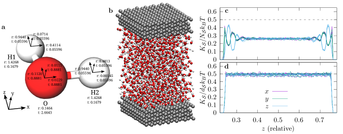
Figure 1: Directional DoF calculation and local temperature measurement of rigid SPC/E [12] water molecules. (a) Example results for the rotational, r, and translational, t, DoF in each Cartesian direction (on axes) and in total (below atom labels) for a water molecule lying in the $xy$-plane with the $x$ axis aligned with the O–H2 bond. (b) Illustrates the test system, (c) shows the directional kinetic energy of hydrogen atoms in each subvolume, $K_{\mathcal{S}}$, normalised by the number of hydrogen atoms in that subvolume, $N_{\mathcal{S}}$ (i.e. neglecting constraints), and (d) shows the same normalised instead by the total hydrogen DoF in the relevant direction within the subvolume, $d_{\mathcal{S}}$. Dashed lines in (c) and (d) indicate the expected value of $0.5k_{B}T$ per DoF, and five 200-ps averages (1 ns trajectory in total) have been superimposed for each observable.

The above is sufficient to calculate the total DoF associated with particle $j$ in a rigid body as

$$d_{j}=\sum_{\alpha\in\mathcal{D}}d_{j}^{\text{tr},\alpha}+\sum_{\begin{subarray}{c}\beta\in\mathcal{D}\\ \mathbf{\hat{q}}_{i\beta}\neq\mathbf{0}\end{subarray}}d_{j}^{\text{rot},\beta},$$ (20)

and hence to obtain the local temperature $T_{\mathcal{S}}$ from Eqn. 1 based on

$$d_{\mathcal{S}}=\sum_{j\in\mathcal{S}}d_{j}.$$ (21)

This is a generalisation of the method presented in Ref. [9] for rigid water molecules viewed from a modal reference frame, and the result is equivalent to that recently derived by Matsubara et al. [13] based on equilibrium statistical mechanics. Directly applying these equations to the same rigid body geometry of the simple point charge extended (SPC/E) water model [12] yields identical values of 1.5947 and 2.8106 DoF for H and O atoms, respectively, regardless of the reference coordinate system. Furthermore, testing on other geometries confirmed that symmetrically equivalent particles within a rigid body are always assigned equal DoF. Further validation by simulation of rigid ethane molecules in contact with a flexible graphene membrane can be seen in Appendix S1, where we note in passing that a small (0.5 fs) timestep was required to avoid drift in the total energy under the NVE ensemble. We attribute this to similar integration issues as those described in detail by Asthagiri et al. [14].

We now extend to consider local temperature measurements along an arbitrary set of mutually orthogonal unit vectors, $\mathbf{\hat{e}}_{\gamma}$, which are not necessarily aligned with the basis vectors of the reference frame, $\mathbf{\hat{e}}_{\alpha}$. For translational DoF, it is trivial to see from projection of each mode along each $\mathbf{\hat{e}}_{\gamma}$ that

$$d_{j}^{\text{tr},\gamma} = \sum_{\alpha\in\mathcal{D}}d_{j}^{\text{tr},\alpha\gamma}$$ (22)

$$= \sum_{\alpha\in\mathcal{D}}\frac{\mathbf{\hat{e}}_{\alpha}^{T}\mathbf{\hat{e}}_{\gamma}\mathbf{\hat{e}}_{\gamma}^{T}\left(m_{j}\mathbf{1}\right)\mathbf{\hat{e}}_{\gamma}\mathbf{\hat{e}}_{\gamma}^{T}\mathbf{\hat{e}}_{\alpha}}{\mathbf{\hat{e}}_{\alpha}^{T}\mathbf{\hat{e}}_{\gamma}\mathbf{\hat{e}}_{\gamma}^{T}\mathbf{M}_{i}\mathbf{\hat{e}}_{\gamma}\mathbf{\hat{e}}_{\gamma}^{T}\mathbf{\hat{e}}_{\alpha}},$$ (23)

$$= \frac{m_{j}}{\sum_{k\in\mathcal{R}_{i}}m_{k}},$$ (24)

and therefore, as expected, the partitioning of translational DoF is invariant to rotation of the coordinate system.

To find the DoF of particle $j$ associated with motion in direction $\gamma$ due to rotational mode $\beta$, Eqn. 19 can be decomposed in a similar manner to obtain the directional inertia of each mode. For rotational motion in mode $\beta$ with angular velocity of magnitude $a$, the velocity of particle $j\in\mathcal{R}_{i}$, projected along direction $\gamma$, is given by

$$v_{j}^{\text{rot},\beta\gamma}=a\left[-\mathbf{r}_{ij,\times}\right]\mathbf{\hat{q}}_{i\beta}\cdot\mathbf{\hat{e}}_{\gamma},$$ (25)

and hence the inertia of that particle in direction $\gamma$ of mode $\beta$ is

$$I_{j}^{\text{rot},\beta\gamma} = m_{j}\frac{\left(v_{j}^{\text{rot},\beta\gamma}\right)^{2}}{a^{2}},$$ (26)

$$= m_{j}\left(\left[-\mathbf{r}_{ij,\times}\right]\mathbf{\hat{q}}_{i\beta}\cdot\mathbf{\hat{e}}_{\gamma}\right)^{2}.$$ (27)

As before, the fractional DoF associated with motion in mode $\beta$ of particle $j$ in direction $\gamma$ is obtained from the relative inertia contribution as

$$d_{j}^{\text{rot},\beta\gamma}=\frac{I_{j}^{\text{rot},\beta\gamma}}{\mathbf{\hat{q}}_{i\beta}^{T}\mathbf{I}_{i}\mathbf{\hat{q}}_{i\beta}}.$$ (28)

Summing over all translational and rotational modes as before yields the total DoF of particle $j$ for motion in direction $\gamma$,

$$d_{j}^{\gamma}=\sum_{\alpha\in\mathcal{D}}d_{j}^{\text{tr},\alpha\gamma}+\sum_{\begin{subarray}{c}\beta\in\mathcal{D}\\ \mathbf{\hat{q}}_{i\beta}\neq\mathbf{0}\end{subarray}}d_{j}^{\text{rot},\beta\gamma},$$ (29)

and hence the directional kinetic temperature of a subset of particles, $\mathcal{S}$, measured along some set of mutually orthogonal $\mathbf{\hat{e}}_{\gamma}$ for $\gamma\in\mathcal{G}$ can be obtained from

$$T_{\mathcal{S},\mathcal{G}}=\frac{\sum_{j\in\mathcal{S}}\sum_{\gamma\in\mathcal{G}}m_{j}\left(\mathbf{v}_{j}\cdot\mathbf{\hat{e}}_{\gamma}\right)^{2}}{k_{B}\sum_{j\in\mathcal{S}}\sum_{\gamma\in\mathcal{G}}d_{j}^{\gamma}}.$$ (30)

An example calculation of the directional DoF of atoms in a rigid water molecule is shown in Fig. 1a. Note, although the two hydrogen atoms are symmetrically equivalent and their total rotational and translational DoF are the same, the directional DoF components are different. This is because the reference frame is not a modal frame.

We validate this directional DoF decomposition by analysing the local, directional kinetic temperature of hydrogen atoms in rigid water molecules confined between two walls, as illustrated in Fig. 1b (Appendix S2 for simulation details). Figure 1c shows that due to ordering of the water molecules near the walls, kinetic energy is not equally partitioned between Cartesian directions. Considering that the system is at equilibrium, and therefore equipartition of energy is expected, it is clear that ordering at the interface causes some directions to have different DoF to others. In Fig. 1d, we introduce a scaling factor equal to the total DoF in the given local volume for motion in the given direction, which is dynamically calculated based on the orientation of each water molecule. This clearly shows that $\left<T_{\mathcal{S},\gamma}\right>=T$, $\forall$ $\gamma\in\mathcal{D}$, $\mathcal{S}\subseteq\mathcal{P}$, as expected at equilibrium.

It is interesting to consider that while this formalism has been derived in terms of rigid bodies composed of point masses, it could be equally applied to volumetric rigid bodies described by a mass density function, $\rho_{i}(\mathbf{r})$. It is simple to see that the density of DoF for translational modes in direction $\alpha$ is given by

$$d_{i}^{\text{tr},\alpha}(\mathbf{r})=\frac{\rho_{i}(\mathbf{r})}{\iiint_{-\infty}^{\infty}d^{3}\mathbf{r}\rho_{i}(\mathbf{r})}.$$ (31)

Similarly, the rotational DoF density of mode $\beta$ is given by

$$d_{i}^{\text{rot},\beta}(\mathbf{r})=\frac{\mathbf{\hat{q}}_{i\beta}^{T}\mathbf{I}_{i}(\mathbf{r})\mathbf{\hat{q}}_{i\beta}}{\mathbf{\hat{q}}_{i\beta}^{T}\mathbf{I}_{i}\mathbf{\hat{q}}_{i\beta}},$$ (32)

where $\mathbf{I}_{i}(\mathbf{r})$ is the density of rotational inertia (see Appendix S4 for details), giving the total density of DoF for rigid body $i$ as

$$d_{i}(\mathbf{r})=\sum_{\alpha\in\mathcal{D}}d_{i}^{\text{tr},\alpha}(\mathbf{r})+\sum_{\begin{subarray}{c}\beta\in\mathcal{D}\\ \mathbf{\hat{q}}_{i\beta}\neq\mathbf{0}\end{subarray}}d_{i}^{\text{rot},\beta}(\mathbf{r}).$$ (33)

From this, the kinetic temperature in a subvolume, $\mathcal{V}$, of a system containing $N$ rigid bodies can be obtained as

$$T_{\mathcal{V}}=\frac{\iiint_{\mathcal{V}}d^{3}\mathbf{r}\sum_{i=1}^{N}\rho_{i}(\mathbf{r})\mathbf{v}_{i}(\mathbf{r})\cdot\mathbf{v}_{i}(\mathbf{r})}{k_{B}\iiint_{\mathcal{V}}d^{3}\mathbf{r}\sum_{i=1}^{N}d_{i}(\mathbf{r})},$$ (34)

where $\mathbf{v}_{i}(\mathbf{r})$ is the velocity induced at position $\mathbf{r}$ due to the combined translational and rotational motion of rigid body $i$. This reduces to the previous consideration of point mass rigid bodies when $\rho_{i}(\mathbf{r})$ is a sum of Dirac delta functions.

An intriguing consequence of this formalism is the possibility to observe a temperature gradient across a rigid body in a system undergoing heat flow by measuring kinetic temperature in subvolumes which are relatively small. This can be simply tested using rigid dumbbells consisting of two particles; one interacting with a bath of hot particles, and one with a bath of cold particles, as illustrated in Fig. 2a. The hot and cold bath particles occupy the same physical space but do not interact directly, hence heat transfer must occur through the rigid dumbbells. Details of the simulations are described in Appendix S3.

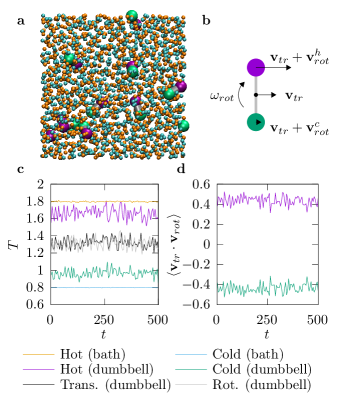
Figure 2: Demonstration of temperature gradient across rigid dumbbells. Panel (a) shows a snapshot of the molecular dynamics simulation. The purple (green) particle of each dumbbell interacts only with particles of the same color and with the orange (cyan) bath particles. Orange bath particles are thermostatted to a normalised temperature of 1.8, and cyan particles a temperature of 0.8. All particles are the same size and mass, although dumbbells are drawn larger for clarity. (b) Illustrates a situation in which one end of a dumbbell carries more kinetic energy than the other, despite excitations of the rotational and translational modes being of similar magnitude. (c) Shows the kinetic temperature of bath and dumbbell particles, and of the translational and rotational dumbbell modes, plotted with time at the steady state (averaged over bins of 5 LJ time units for clarity). Similarly, (d) shows the correlation between the translational and rotational velocity components of the hot and cold dumbbell particles, averaged over the 10 dumbbells in the system.

Figure 2c shows the kinetic temperatures of the baths, the hot and cold ends of the dumbbells, and the translational and rotational modes of the dumbbells in the steady state. It can be seen that while the overall translational and rotational temperatures of the dumbbells are approximately equal, the dumbbell particles in contact with the hot bath have significantly more kinetic energy on average than the ones in contact with the cold bath. This implies some correlation between the translational and rotational velocity components, resulting in a situation which is on average similar to that illustrated in Fig. 2b. Figure 2d plots the correlation function between the velocity component of a particle in a rigid dumbbell due to translation and that due to rotation, clearly showing a positive correlation for the hot particle, and a negative one for the cold particle. Thus, the rigid body motion is such that one end of the dumbbell is consistently and significantly hotter than the other.

While these partial and local temperature measurements are in principle suitable for use with a thermostat, it is important to note that (1) the thermostat should only be applied to the motion contributing to the temperature measurement, and (2) for rigid bodies undergoing flow, both translational and rotational streaming motion in the directions of interest must be subtracted before measuring the kinetic temperature. Point (2) is particularly important; even if kinetic temperature is measured only in directions perpendicular to the flow, rotational motion (e.g. under shear flow) can contribute to the velocities being measured, and hence the streaming angular momentum must still be accounted for.

Finally, we note that this framework can be extended in a practical manner to arbitrary sets of constraints by considering an internal coordinate system for semi-rigid fragments such that the constraints are implicit. The kinetic energy of a semi-rigid fragment, $i$, consisting of the set of particles $j\in\mathcal{F}_{i}$ is given by [15]

$$K_{i}=\frac{1}{2}\dot{\bm{\theta}}_{i}^{T}\bm{\mathcal{I}}_{i}\dot{\bm{\theta}}_{i}=\frac{1}{2}\dot{\bm{\theta}}_{i}^{T}\mathbf{J}_{i}^{T}\left[\begin{array}[]{ccc}m_{1}\mathbf{1}&\cdots&\mathbf{0}\\ \vdots&\ddots&\vdots\\ \mathbf{0}&\cdots&m_{j}\mathbf{1}\end{array}\right]\mathbf{J}_{i}\dot{\bm{\theta}}_{i},$$ (35)

where $\dot{\bm{\theta}}_{i}$ is the velocity in the internal coordinate system, $\bm{\mathcal{I}}_{i}$ is the inertia, and $\mathbf{J}_{i}$ is the Jacobian with rank equal to the total DoF which transforms from internal coordinate velocities to lab-frame particle velocities. It has been shown that internal coordinate systems, when transformed to the modal frame, satisfy the equipartition theorem [16]. With, again, the eigenvectors, $\mathbf{\hat{q}}_{i\beta}$ of the generalised inertia $\bm{\mathcal{I}}_{i}$ as columns of $\mathbf{Q}_{i}$, the generalised velocity in the modal frame is given by $\mathbf{Q}_{i}^{T}\dot{\bm{\theta}}_{i}$, and the modal inertia is $\mathbf{Q}_{i}^{T}\mathbf{J}_{i}^{T}\bm{\mathcal{M}_{i}}\mathbf{J}_{i}\mathbf{Q}_{i}$, where $\bm{\mathcal{M}}_{i}$ is the mass matrix in Eqn. 35. As in previously considered examples, self-consistency dictates that the DoF associated with the motion of particle $j$ in a particular mode is given by its contribution to the modal inertia, which may be calculated for mode $\beta$ by $\mathbf{\hat{q}}_{i\beta}^{T}\mathbf{J}_{i}^{T}\bm{\mathcal{M}}_{ij}\mathbf{J}_{i}\mathbf{\hat{q}}_{i\beta}$, where $\bm{\mathcal{M}}_{i}=\sum_{j\in\mathcal{F}_{i}}\bm{\mathcal{M}}_{ij}$. However, in this case, the matrix $\mathbf{J}_{i}$ depends on the particular configuration, and hence the DoF of a given particle may change with time during a simulation, as was noted by Matsubara et al. [13]. We leave application of this method to semi-rigid fragments as future work.

In summary, we have derived a self-consistent framework for partitioning the degree of freedom associated with a given mode between participating masses by requiring only that any subset of masses has the same kinetic temperature within the mode. This leads to the simple result that the fraction of a mode’s DoF associated with a particular mass is equal to the inertia of that mass in the modal motion divided by the total inertia of the mode. This enables both local and directional kinetic temperature measurement, and is applicable both to point masses and to volumetric rigid or semi-rigid bodies. Results were validated on molecular dynamics simulations of rigid bodies in inhomogeneous systems, where the utility of the method is evident. Importantly, this method is general over arbitrarily constrained systems, and enables local kinetic temperature measurements which encompass all relevant DoF.

APPENDIX

Appendix S1 Validation on rigid bodies

As a simple prototypical inhomogeneous test system, we model 500 rigid ethane molecules in contact with a flexible 7-layer graphene membrane inside a $3.92\times 3.82\times 5.5$ nm³ periodic unit cell (see Fig. S3a). This gives a system with two regions having approximately equal number density of atoms, but with all rigid constraints concentrated in the ethane phase. Moltemplate [17] was used to generate the initial configuration and LAMMPS [18] (version June 2023) to simulate the dynamics using the rigid integrator. Ethane geometry and interaction parameters were from the automated topology builder [19, 20] based on the GROMOS 54A7 forcefield [21], “make graphitics” [22] was used to generate the graphene membrane, and geometric mixing rules were applied for Lennard-Jones parameters between ethane and graphene. To equilibrate the system at 300 K, we initially apply a Nosé-Hoover thermostat [23] to the atoms in the graphene membrane and a separate Nosé-Hoover thermostat to the rigid ethane molecules, both with a coupling time of 100 fs. After 50 ps with a 0.5 fs integration timestep, we remove the thermostats and further equilibrate for an additional 10 ps in the isoenergetic (NVE) ensemble before measuring the kinetic energy in 15 slabs equally spaced in the $z$ direction (perpendicular to the membrane) over a period of 100 ps. To keep temperature profile data comparable over time, the graphene membrane was restrained in the $z$ direction by coupling its center of mass to a harmonic oscillator with spring constant 5000 kcal mol${}^{-1}\textup{~{}\AA}^{-2}$ at the mid-point of the periodic unit cell. This was done consistently throughout the equilibration and production stages of the simulation. Figure S3b compares the kinetic temperature profile calculated using fractional DoF partitioning as derived in the main text versus the naïve method of assuming that each atom in the system has the same number of DoF (the current default in LAMMPS for computing temperature profiles, and a reasonable approximation for homogeneous systems). These results clearly show that the DoF partitioning scheme yields a uniform kinetic temperature profile as expected, despite the inhomogeneity, while the naïve method, predictably, does not.

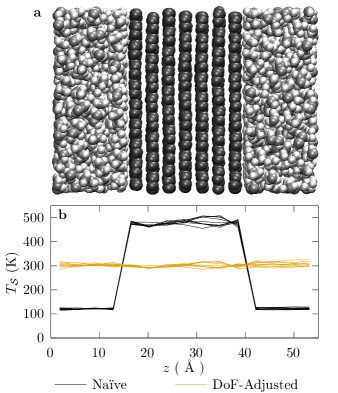
Figure S3: Test of local DoF calculation using rigid ethane molecules in contact with a flexible graphene membrane at equilibrium. A snapshot of the system visualised with VMD [24, 25] is depicted in (a), aligned with the $x$ axis of the plot in (b) which shows the local temperature of 15 equally sized slab subvolumes centered around the corresponding $z$ values. The naïve method calculates local temperature based on the assumption that each atom (whether it is part of a rigid molecule or not) has the same number of DoF associated with it, while the DoF-adjusted method partitions DoF based on each atom’s contribution to the inertia of each mode (3 DoF per graphene carbon atom, 1.75174 per carbon in rigid ethane, and 0.41607 per hydrogen). Each line in (b) represents the average temperature profile over a 10 ps time window.

Appendix S2 Simulation details: confined water

Wall particles were modelled as copper atoms (mass 63.546 amu) on a fcc lattice with (100) surface. Each particle was restrained about its initial lattice position with a three-dimensional harmonic potential of spring constant $k=65$ kcal/(mol.Ų), or a fundamental oscillatory period of about 48 fs. A three-particle chain Nosé-Hoover thermostat was applied to the combined group of upper and lower wall particles with temperature $T=300$ K and coupling time $\tau=100$ fs, using the LAMMPS tloop 5 keyword to integrate the thermostat variables over five substeps per main integration step for added accuracy. Rigid water molecules were of the simple point charge extended (SPC/E) type [12], and were integrated using Newton’s equations of motion. SHAKE, RATTLE (both with $10^{-4}$ relative accuracy), or LAMMPS’ rigid integrator were used to impose constraints, with minimal differences observed between constraint algorithms.

Appendix S3 Simulation details: heat transfer through rigid dumbbells

All particles, including those that formed the rigid dumbbells, were simple Lennard-Jones (LJ) particles of unit size and mass with an interaction cut-off of 2.6 LJ units. The hot and cold particles were coupled to separate Nosé-Hoover thermostats at $T_{H}=1.8$ and $T_{C}=0.8$, respectively, with a coupling time of $0.1$, all in normalised LJ units. The cubic periodic unit cell of side length 10.77 LJ units contained 990 hot particles, 990 cold particles, and 10 dumbbells with bond length 1.077, for a total effective density of $0.8$ for each set of interacting particles. This ensured that both baths were in the liquid phase. Free particles simply have 3 DoF each, while each particle within a dumbbell has 2.5 DoF (1.5 translational and 1 rotational). Particles were initially generated on a cubic lattice, and then simulated for 250 LJ time units to reach the steady state before gathering data.

Appendix S4 Rotational inertia of volumetric rigid bodies

For a rigid body, $i$, with mass density $\rho_{i}(\mathbf{r})$, the contribution of point $\mathbf{r}$ to the rotational inertia is given by

$$\mathbf{I}_{i}(\mathbf{r})=\rho_{i}(\mathbf{r})\left[(\mathbf{r}-\mathbf{r}_{i})_{\times}\right]^{2},$$ (S36)

where $\mathbf{r}_{i}$ is the center of mass of the rigid body, and the $\times$ subscript is as defined in Eqn. 7 of the main text. The total rotational inertia of the rigid body is then given by

$$\mathbf{I}_{i}=\iiint_{-\infty}^{\infty}d^{3}\mathbf{r}\mathbf{I}_{i}(\mathbf{r}).$$ (S37)

Hence, with $\mathbf{Q}_{i}$ defined as before from the eigenvalues of $\mathbf{I}_{i}$ such that $\mathbf{Q}_{i}^{T}\mathbf{I}_{i}\mathbf{Q}_{i}$ is diagonal, the density of DoF associated with rotational mode $\beta$ can be obtained as for the translational modes from the fractional contribution of a point in space towards the total inertia of the mode,

$$d_{i}^{\text{rot},\beta}(\mathbf{r})=\frac{\mathbf{\hat{q}}_{i\beta}^{T}\mathbf{I}_{i}(\mathbf{r})\mathbf{\hat{q}}_{i\beta}}{\mathbf{\hat{q}}_{i\beta}^{T}\mathbf{I}_{i}\mathbf{\hat{q}}_{i\beta}}.$$ (S38)