Automated optimization of force field parameters against ensemble-averaged measurements with Bayesian Inference of Conformational Populations
Abstract
Accurate force fields are essential for reliable molecular simulations. These models are refined against quantum mechanical calculations and experimental measurements, which are subject to random and systematic errors. Bayesian Inference of Conformational Populations (BICePs) is a reweighting algorithm that reconciles simulated ensembles with sparse or noisy observables by sampling the full posterior distribution of conformational populations and experimental uncertainty. In this method, a metric called the BICePs score is used to perform model selection, by calculating the free energy of "turning on" the conformational populations under experimental restraints. This approach, when used with improved likelihood functions to deal with experimental outliers, can be used for force field validation (Raddi et al. 2023). Here, we extend the BICePs approach to perform automated force field refinement while simultaneously sampling the full distribution of uncertainties, using a variational method to minimize the BICePs score. To demonstrate the utility of this method, we refine multiple interaction parameters for a 12-mer HP lattice model using ensemble-averaged distance measurements as restraints. To illustrate the resilience of BICePs in the presence of unknown random and systematic errors, we assess the performance of our algorithm through repeated optimizations and under various extents of experimental error. Our results suggest that variational optimization of the BICePs score is a promising direction for robust and automatic parameterization of molecular potentials.
I Introduction
The accuracy of physical potentials used in molecular simulations continues to improve, especially as training data for fitting energy surfaces from quantum-mechanical calculations becomes more available.Boothroyd et al. (2023); Smith et al. (2019) Of similar importance is developing models that can accurately predict ensemble-averaged experimental measurements. Parameterizing models for this purpose is a nontrivial task that requires continuous refinement of microscopic parameters through iterated sampling of the equilibrium distribution.
Such refinement often involves global minimization of the deviation between experimental measurements (e.g. NMR observables) and theoretical predictions from simulated ensembles (the “forward model”), with several complications to consider. First, the forward model is itself an approximation containing some error. Second, ensemble-averaged experimental measurements can be sparse and/or noisy, susceptible to random and systematic errors, which are often unknown a priori. Hence, force field refinement requires a mechanism to integrate these multiple sources of uncertainty to automatically discover the optimal parameter set across multiple systems.
Other challenges arise from practical considerations. The high dimensionality and interdependence of force field parameter space presents a significant challenge for refinement. When parameter spaces are large, reproducibility may also be an issue; ideally, identical experimental data should produce parameterizations that should converge towards the same optimal values. For these reasons, automated optimization procedures with sufficiently smooth and differentiable objective functions are preferred.
Numerous methodsKöfinger and Hummer (2021); Wang, Martinez, and Pande (2014); Ge and Voelz (2018); Madin et al. (2022) have been developed to address most of these challenges. However, many algorithms do not include any treatment of uncertainty in the training data, and others lack gradients for automatic refinement. To address these challenges, Bayesian inference methods have been developed.Köfinger and Hummer (2021); Madin et al. (2022); Ge and Voelz (2018) These methods estimate a Bayesian posterior distribution of conformational populations by treating molecular simulation predictions as prior information, weighted by a likelihood function constructed from the experimental measurements and their uncertainties. The Bayesian posterior can then be used to optimize the prior.
In this work, we extend the Bayesian Inference of Conformational Populations (BICePs) algorithmVoelz, Ge, and Raddi (2021); Raddi et al. (2023) to perform automated force field refinement. BICePs is a reweighting algorithm that refines structural ensembles against sparse and/or noisy experimental observables, and has been used in many previous applications.Voelz and Zhou (2014); Wan et al. (2020); Hurley et al. (2021); Raddi, Ge, and Voelz (2023) A key advantage of BICePs is that it does not require uncertainty estimates for the forward model; instead, it infers the posterior distribution of these parameters directly from the data through MCMC sampling. BICePs also computes a free energy-like quantity called the BICePs score that can be used for model selection.Ge and Voelz (2018); Raddi et al. (2023)
More recently, we have equipped BICePs with a replica-averaging forward model, making it a maximum-entropy (MaxEnt) reweighting method, and unique in that no adjustable regularization parameters are required to balance experimental information with the prior.Raddi et al. (2023) With this new approach, the BICePs score becomes a powerful objective function to select and parameterize optimal models. Here, we show that the BICePs score, which reflects the total evidence for a model, can be used for variational optimization of model parameters. The BICePs score contains a form of inherent regularization, and has specialized likelihood functions that allow for the automatic detection and down-weighting of data points subject to systematic error.Raddi et al. (2023)
To efficiently optimize complex parameter spaces, we derive the first and second derivatives of the BICePs score. We then show how to perform automatic force field optimization against ensemble-averaged observables for several test systems, including a protein lattice model with adjustable bead interaction strengths, and a von Mises-distributed polymer model.
II Theory
BICePs uses a Bayesian statistical framework to treat the extent of uncertainty in experimental observables, , as nuisance parameters. Previous versions of BICePs sampled conformational states and uncertainty parameter(s) from the Bayesian posterior, which takes the form
| (1) |
Here, the prior comes from a theoretical model of conformational state populations (typically from a molecular simulation), is a likelihood function quantifying how well a forward model prediction agrees with the experimental data , and is a non-informative Jeffreys prior.
When BICePs is equipped with a replica-averaged forward model, it becomes a MaxEnt reweighting method in the limit of large numbers of replicas Pitera and Chodera (2012); Cavalli, Camilloni, and Vendruscolo (2013); Cesari, Reißer, and Bussi (2018); Roux and Weare (2013); Hummer and Köfinger (2015). The posterior takes the general form
| (2) |
where is a set of conformation replicas, is an observable in the set of ensemble-averaged experimental measurements, and is the replica-averaged forward model prediction of observable . The values are nuisance parameters that capture uncertainty in the measurements as well as the replica-averaged forward model. In (2), a Gaussian likelihood is used, but more sophisticated models of uncertainty can be used to capture outliers and systematic error with fewer parameters, as discussed below. Markov chain Monte Carlo (MCMC) is used to sample the posterior.
The replica-averaged forward model requires a more sophisticated treatment of uncertainty, since it is approximating the ensemble average as a replica average.Bonomi et al. (2016). Therefore, becomes a combination of both the Bayesian error and the standard error of the mean sigma , . The finite sampling error, is estimated by taking a windowed average over our finite sample as , which decreases as the square root of the number of replicas.
II.1 Accounting for systematic error and outliers.
BICePs is equipped with special likelihoods that are very robust in the presence of systematic error. The Student’s likelihood model is a data error model that marginalizes the uncertainty parameters for individual observables, assuming that the level of noise is mostly uniform, except for a few erratic measurements. This limits the number of uncertainty parameters that need to be sampled, while still capturing outliers.
Consider a model where uncertainties for particular observables are distributed about some typical uncertainty according to a conditional probability . We derive a posterior with a single uncertainty parameter by marginalizing over all . For a single replica (for simplicity), the posterior is given by
| (3) |
where .
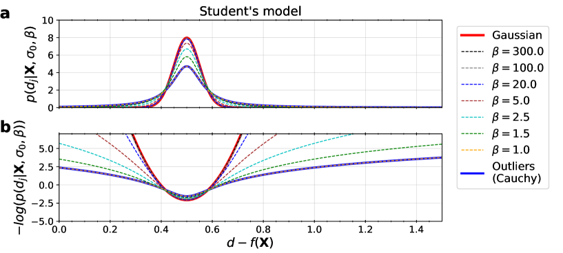
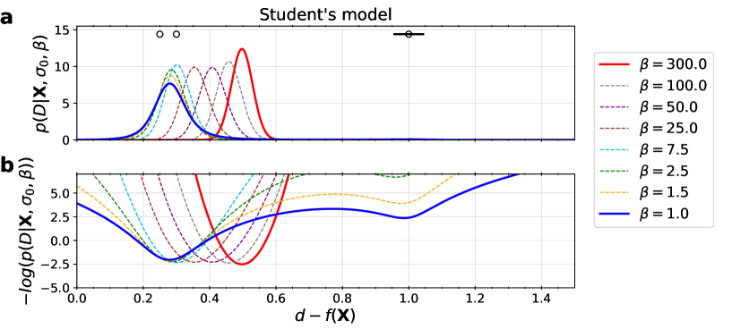
Modeling the prior on uncertainties with a distribution with long tails is very useful because its long tail makes it able to tolerate outliersSivia and Skilling (2006); Bonomi et al. (2016). In most cases, however, it is unclear a priori what distribution is best for modeling the input data. To improve the situation, we introduce a model with an additional nuisance parameter , that is able to tune the extent of the distribution’s tail:
| (4) |
where is defined as above, and . When this distribution is inserted into the posterior, and marginalized over all , the result is
| (5) |
Here, the marginal likelihood contains the lower incomplete gamma function, . We call this the Student’s model because it is a variation of Student’s -distribution that can be interpolated between functional forms. When , the model is equivalent Metainference’s Outliers modelBonomi et al. (2016). In the limit of , the likelihood becomes Gaussian. When considering the full posterior, this extra nuisance parameter is given a non-informative Jeffreys prior, . For more details regarding the Student’s model, see Figures S1-S2.
II.2 The BICePs score: a tool for quantitative model selection and refinement
The BICePs score is a free energy-like quantity that rigorously characterizes model quality. For a model of prior populations parameterized by , with corresponding prior energy , the BICePs score is calculated as the negative logarithm of a Bayes factor,
| (6) |
is the total evidence of the specified model, marginalized over all conformational replicas and uncertainty. By defining the BICePs energy function as , it takes the form
| (7) |
is defined similarly, but for a uniform prior that does not depend on . thus serves as a well-defined reference state. By constructing a series of intermediates that scale the prior as , the BICePs score is calculated as the change in free energy for “turning on” the prior (Figure 1).
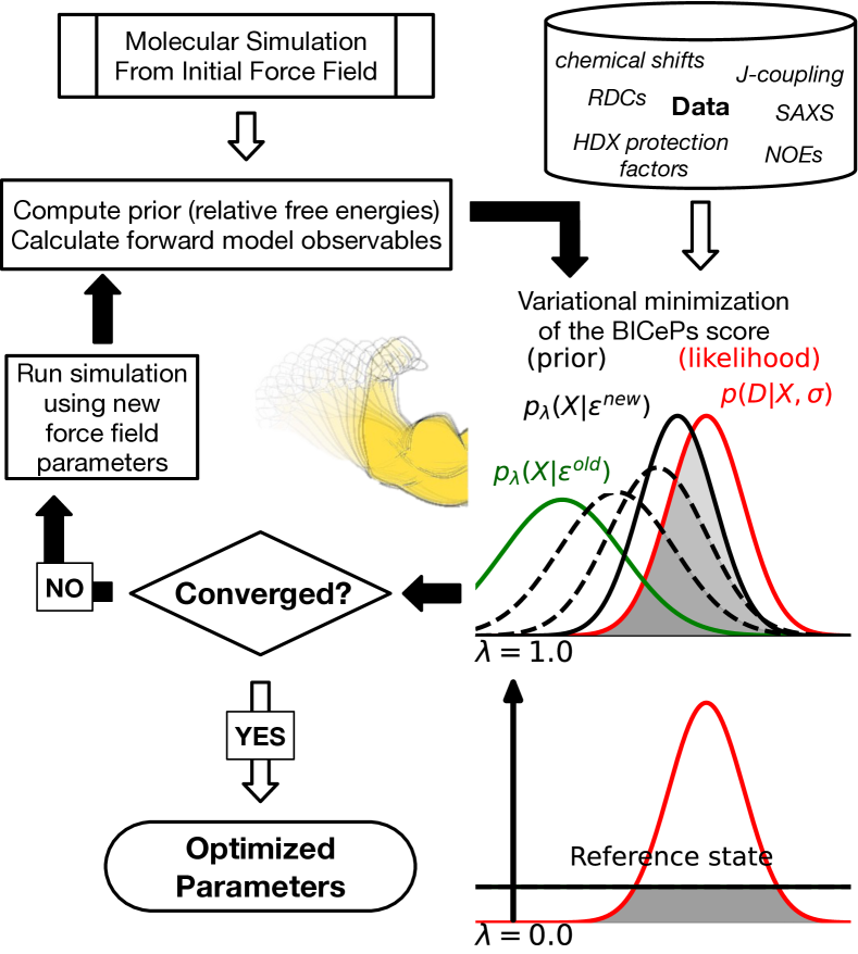
II.3 Variational minimization of the BICePs score to find optimal model parameters.
We assume there exists some posterior distribution with the maximal evidence, derived from optimal parameters . In this case, the free energy is a global minimum, and any other set of parameters has .
Our objective is to find starting with trial parameters and corresponding distribution . To do this, we iteratively perform BICePs calculations to estimate , then update the parameters to further minimize this quantity, until the stopping criteria is reached. Given a differentiable prior, is also differentiable, enabling application of any number of gradient-based convex optimization schemes, with a stopping criteria of , within some tolerance.
The derivative of the BICePs score with respect to parameters reduces to the ensemble-averaged value of ,
| (8) |
where
| (9) |
The reference ensemble does not affect the gradient of , since a uniform prior is independent of , and is zero (see section Automated optimization of force field parameters against ensemble-averaged measurements with Bayesian Inference of Conformational Populations for more details).
The second partial derivatives of the BICePs score with respect to parameters and are:
| (10) | ||||
where the notation denotes the ensemble average with respect to . The first term on the right is the ensemble-averaged second derivative of the energy function with respect parameters and :
| (11) |
When = , the second partial derivative of the BICePs score reduces to the difference between the ensemble-averaged second derivative of the energy and the variance of its first partial derivative:
| (12) |
In practice, all of these quantities are estimated as ensemble-averaged observables at the same time is estimated, using the MBAR free energy estimator. MCMC sampling at several intermediates enables accurate estimates of all quantities (Figure 1).
III Methods
III.1 A toy protein lattice model
The HP lattice model of Dill and ChanDill et al. (1995) is a simplified protein folding model that represents a protein sequence as a chain of beads on a 2-D square lattice. In this model, each amino acid residue is classified as either a hydrophobic (H) or polar (P) bead. Each microscopic chain conformation has an energy proportional to the number of H-H contacts ,
| (13) |
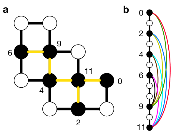
A “contact” is defined as a non-sequential pair of hydrophobic residues at adjacent lattice sites. As a test system, we consider a 12-mer protein sequence HPHPHPHPPHPH (Figure 2a) . When is sufficiently large, there is a single lowest-energy microstate that corresponds to the global free energy minimum; such sequences are deemed foldable. For the 12-mer HPHPHPHPPHPH sequence, there are 15037 unique microstate conformations that can be binned into 72 macrostates, each with a unique set of contacts.
To explore a system with multiple parameters, we modify the HP model to include multiple interactions. Each bead with sequence position is assigned a unique interaction strength, , and a geometric-average combination rule is used to compute the energy of each microstate:
| (14) |
where the sum is taken over all pairs of residues that are in contact.
The first derivative of the contact energy with respect to is given by
| (15) |
and the second derivative of the contact energy with respect to and is given by:
| (16) |
We use the 72 macrostates with unique contacts as a set of prior populations for use with BICePs. For each macrostate , the populations are computed as
| (17) |
where is the reduced energy (in units ) of each microstate in macrostate , and is the multiplicity (the number of microstates belonging to macrostate ).
The ensemble-averaged distance observables for each macrostate (and their variance over all microstates belonging to it) are computed as follows. Let represent the average distance between residues and in the macrostate. Then, the ensemble-averaged distance observables are given by:
| (18) |
and the variance of the distance observables is given by:
| (19) |
where is the variance of the average distance between residues and in the macrostate.
For ease of interpretation, we assume that the distance units of the square lattice are Ångstroms (1Å= m).
IV Results and Discussion
IV.1 The BICePs score landscape correctly identifies optimal parameters for an HP lattice model.
To understand BICePs’ ability to learn optimal parameters, we start by scanning the BICePs score landscape over a single parameter. For this purpose, we use an HP model where all six hydrophobic beads share the same value of .
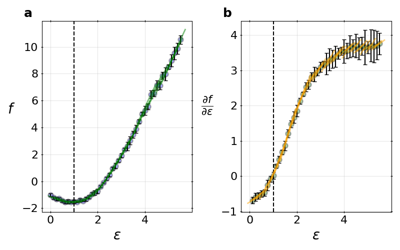
To generate a set of experimental distance observables for testing, we set the "true" value of to 1.0., and compute average distances and variances of eight distances for each macrostate (Figure 2b). The BICePs score and its first and second derivatives are then evaluated across a range of values, spanning from 0.0 to 5.5, in increments of 0.125, where prior energies are unique for each value. BICePs scores and derivatives are averaged over five independent calculations using 100k steps of MCMC with 8 replicas. The associated error bars represent the standard error of the mean across these five instances.
The resulting landscape pinpoints the optimal parameter as a minimum, and correctly computes the first and second derivatives (Figure 3). Despite the stochastic sampling inherent to BICePs, the BICePs score landscape is remarkably smooth and precise, revealing the optimal epsilon to be , the value with the lowest BICePs score, (Figure 3a.), with its derivative at this location equal to 0.0 (Figure 3b.). This optimal model is achieved when the overlap between the likelihood and prior distributions is maximized (Figure 1). When is significantly larger than the true value, the uncertainty in and increases. In this case, the physical interpretation is that for large values of the 12-mer primarily populates the folded macrostate, which results in poor overlap between the likelihood and prior, and more finite sampling error.
IV.2 Automated optimization schemes.
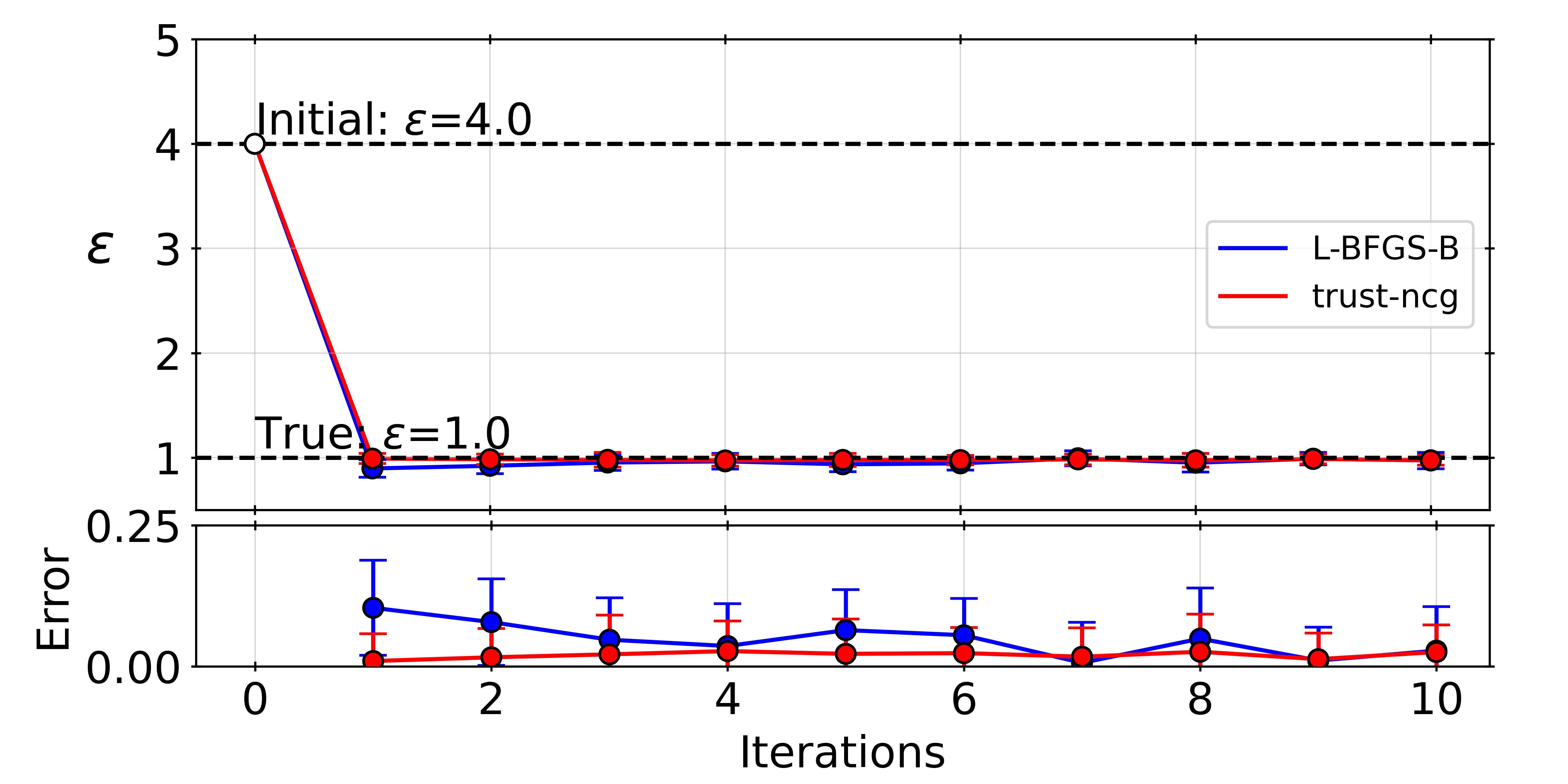
With the ability to compute first and second derivatives of the BICePs score, we next explored the performance of automated optimization methods L-BFGS-BByrd et al. (1995) and Trust-NCGWright (2006) on the single- system. L-BFGS-B is a first-order approach that uses information from gradients, while Trust-NCG is a second-order approach that additionally makes use of information from the Hessian. All default optimization parameters from SciPy were used except a value of ftol=1e-8 (default: ftol=1e-9), and the bounds for each parameter to be optimized was set to be in the range [0, 10]. With only a single parameter, automatic refinement using both optimization methods quickly finds the minimum in a single iteration (Figure S3). However, use of the Hessian (second-order) enables faster convergence, and tends to be slightly more robust for this particular example.
IV.3 The Student’s model confers resiliency when dealing with experimental error.
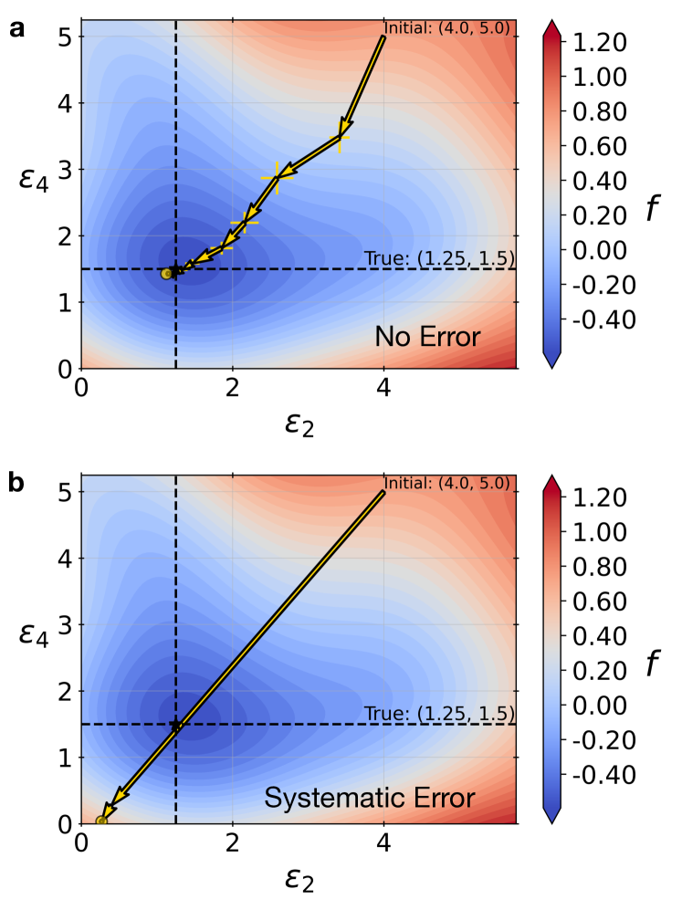
We next examined the robustness of the BICePs score to errors and uncertainties present in experimental data, by introducing random and systematic errors to the 2–11 and 0–11 distance observables (Figure S4). When we used BICePs with a standard Gaussian likelihood model in which a single uncertainty parameter is used for all experimental observables, introducing random and systematic errors significantly reduces the accuracy of the model. When 2–11 and 0–11 distances are perturbed by +3 to +5 Å, the BICePs score predicts a value of smaller than the “true” value, predicting structures that are primarily "unfolded". This in turn causes a leftward shift in the gradient plot (Figure 3b).
In contrast, the Student’s likelihood model deals with the outliers much more handily. The minimum BICePs score correctly identifies the optimal value of , and the leftward shift in the gradient plot is absent. The Student’s model is able to automatically identify outliers directly from the input data, and mitigate their influence, even when 25% of the data (2 of the 8 distances) are corrupted.
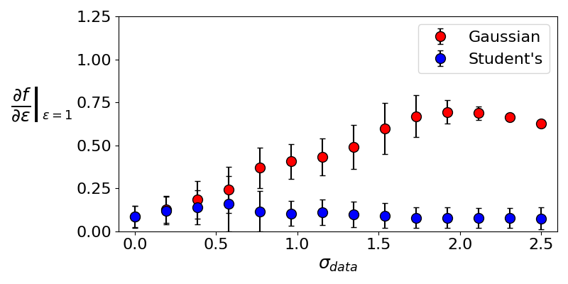
To more critically assess the performance of the Gaussian and Student’s models in dealing with systematic errors, we examine the extent to which the gradient of the BICePs score deviates from zero at the “true” value of . We introduced random perturbations to the 2–11 and 0–11 distances of various standard deviations, (Figure 4). When the Gaussian likelihood model was used, the computed gradient at increases proportionally with the magnitude of ., and becomes particularly unreliable when the error surpasses 0.75 Å. When the Student’s model was used, however, we find that such deviations are reduced. As increases from zero, the gradient at begins to increase, but then begins to decrease beyond = 0.6 Å. This happens because the perturbations in the distance observables become large enough to be detected as outliers by the Student’s model.
IV.4 Multiparameter optimization
While our toy protein lattice model is very simple, the inference problem it presents is challenging, especially as we increase the number of epsilon parameters to refine. Our 12-mer system has only eight experimental distances as experimental restraints, and these are significantly influenced by ensemble-averaging. Moreover, the protein lattice model has a highly cooperative folding landscape, which can lead to correlated distance restraints that don’t independently provide informative insights.
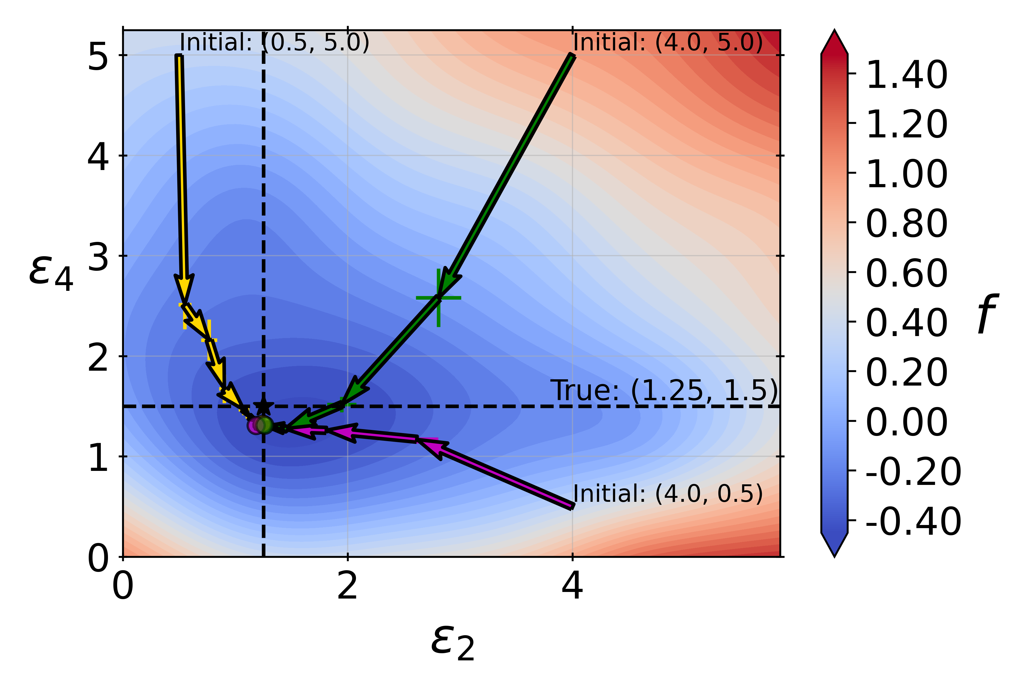
With this in mind, we further tested multi-parameter minimization of the BICePs score, using the modified HP lattice model with tunable interaction strengths . Ideally, our algorithm should be able to efficiently find the global minimum of starting from many different initial parameter sets, and be resilient against random and systematic errors. For two or more parameters, it becomes computationally expensive to perform multidimensional scans of the BICePs score landscape, necessitating automated parameter optimization.
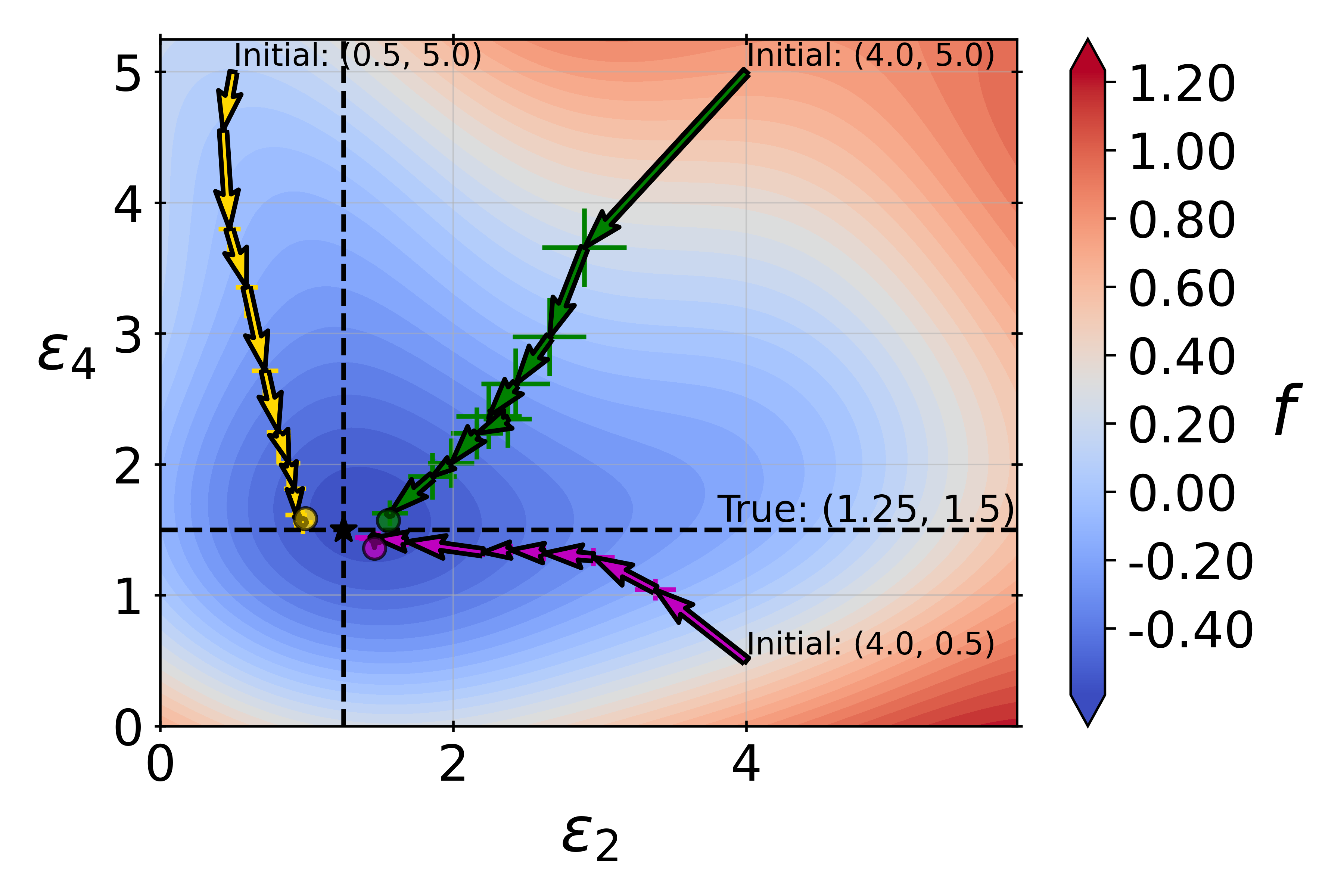
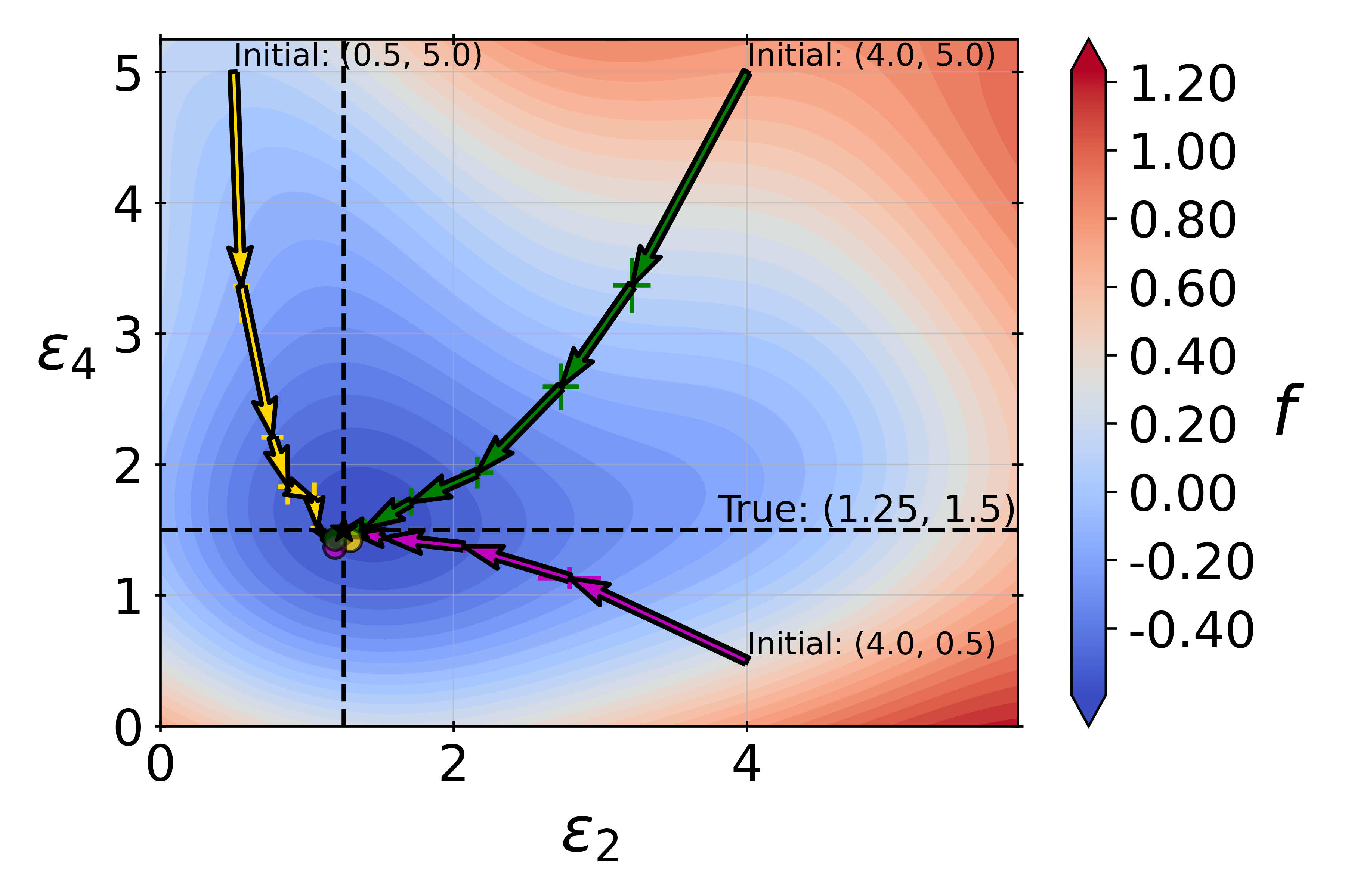
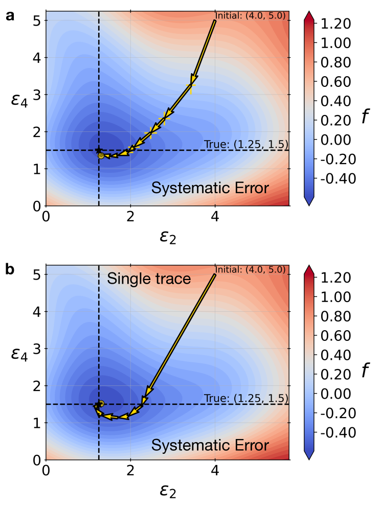
We first generated test data for a model where we set the “true” values to and the remaining set to 3.0. We then tested two-parameter optimizations, starting from three different initial parameter sets = , using both L-BFGS-B and ‘trust-ncg’ optimization for BICePs scores calculated using 8 replicas. Optimizations using L-BFGS-B are unable to fully reach the “true” values of the interaction strength parameters (, ) within 10 iterations (Figure S5). The ‘trust-ncg’ optimization, however, successfully found the correct minima within 10 iterations, demonstrating the notable advantage of second-order methods (Figure S6).
To visualize the two-parameter BICePs score landscape , we constructed a smooth 2-D landscape by averaging five repeated evaluations over a (66) set of grid points, and trained a Gaussian process regression on the grid values using an RBF kernel. The landscape matches the computed BICePs scores, and shows that trajectories of successive () values correctly follow gradients, normal to the landscape contour lines.
The reported uncertainties in the optimized values comes from an estimation of the covariance through inversion of the Hessian (the matrix of second partial derivatives of the BICePs score):
| (20) |
Conceptually, this means that the estimated uncertainties in the best-fit values represent the widths of the basins on the BICePs score landscape. This can sometimes lead to an overestimation of the uncertainty with trust-region optimization schemes, especially with flatter basins like those we observe in the BICePs score landscape. Conversely, the sharper the curvature (larger eigenvalues of the Hessian), the more certain we are about the location of the minimum in that direction, resulting in smaller computed uncertainties. Inspection of Equations (9), (12) and (39) show that , where is the number of BICePs replicas. This suggests that one can obtain smaller uncertainties in the optimized parameters by using more replicas (albeit at greater computational expense). Indeed, repeating the ‘trust-ncg’ optimization with 32 BICePs replicas results in average optimized parameters of = 1.12 0.39, and = 1.43 0.34, which have smaller uncertainty estimates compared to the calculations made with 16 replicas ( = 0.59, and = 0.47). (Figure S7).
In all our multiparameter optimizations, we use a standardized convergence criterion, determined by assessing the average relative change between the old parameters and the new parameters at each iteration, calculated as
| (21) |
where convergence is considered to have been reached when the average change in parameters is less than 0.05. In addition, we strictly require that the convergence condition is satisfied three times in succession.
IV.5 Multiparameter optimization in the presence of systematic error
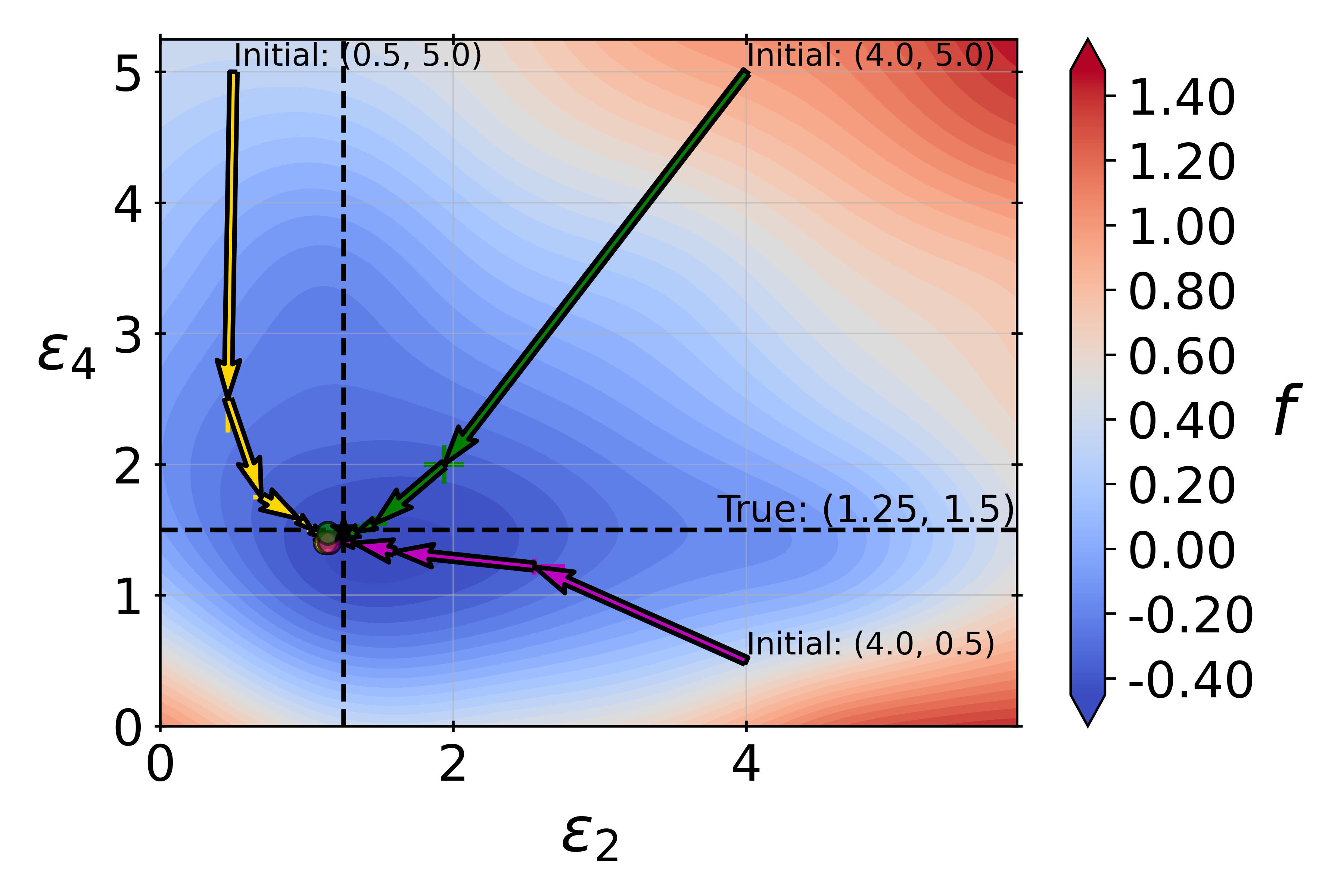
To assess the resiliency of multiparameter optimization to systematic error, we added extra complexity to the optimization problem by introducing systematic error of +3 Å and +3.5 Å to the 2–11 and 4–9 distances observables, respectively. This makes total error in the data Å, a significant obstacle to the refinement of parameters and , considering these beads each participate in only two of measured distances (Figure 2b).
We performed ‘trust-ncg’ optimization using the Student’s model with 200k MCMC steps and 32 replicas, starting from three different initial parameters: = (Figure 5). Indeed, repeating the ‘trust-ncg’ optimization with 32 BICePs replicas results in average optimized parameters of = 1.24 0.41, and = 1.31 0.33, which have smaller uncertainty estimates compared to the calculations made with 16 replicas ( = 1.28 0.59, and = 1.31 0.47). Notably, this was achieved in only a few iterations, showing the algorithm’s proficiency in finding the optimal parameters, irrespective of the initial reference parameters.
In adherence to best practicesBeiranvand, Hare, and Lucet (2017), we compute accuracy profiles for two-parameter ‘trust-ncg’ optimizations using 32 BICePs replicas with no systematic error (Figure S8) and systematic error (Figure S9). The accuracy profiles show the relative error as a function of number of iterations. Optimizations with no systematic error were repeated using only 16 BICePs replicas (Figure S10). A comparison of the 16-replica and 32-replica results shows that the variance between independent optimization traces decreases as the number of replicas increases. The error bars plotted in the accuracy profiles report uncertainties estimated from the inverse Hessian. In each case, it can be seen that the actual variation in the relative error across many optimizations is well within the Hessian-estimated uncertainty.
As we did with the one-parameter optimizations, we also examined the performance of two-parameter optimizations when using a standard Gaussian likelihood model, in the absence of systematic error (Figure S11a) and in the presence of systematic error (Figure S11b). As before, we find that the accuracy of the refined parameters drops significantly when using a standard Gaussian likelihood model. With only a single parameter to estimate the uncertainty in the data set of distances, the Gaussian likelihood model is unable to properly detect the two outliers, and as a result predicts optimal and values that are much smaller than the “true” values. Conversely, the accuracy of the Student’s model is very robust in the presence of systematic error (Figure S12). These results yet again highlight the ability of BICePs to handle uncertainties and systematic error comprehensively when used with a likelihood model that can deal with outliers.
IV.6 Performance in higher-dimensional parameter landscapes
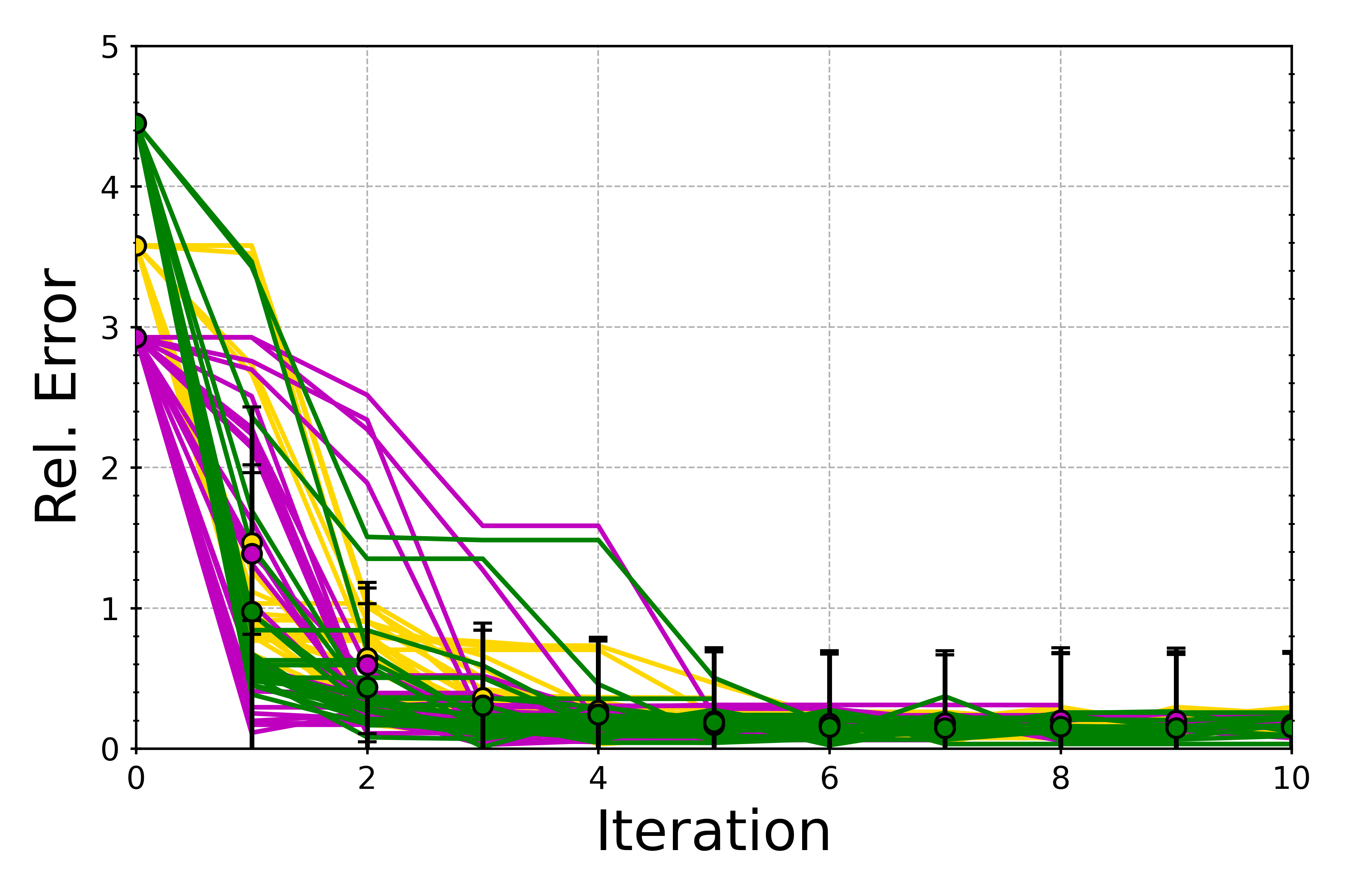
We next attempted to optimize a three-parameter BICePs score landscape, by introducing an additional parameter, . This is a challenging task that may take many iterations to reach the convergence criteria. Our objective was to examine the typical percentage of optimization traces that converge within a designated number of iterations. For this test, we refrained from adding systematic error to the data.
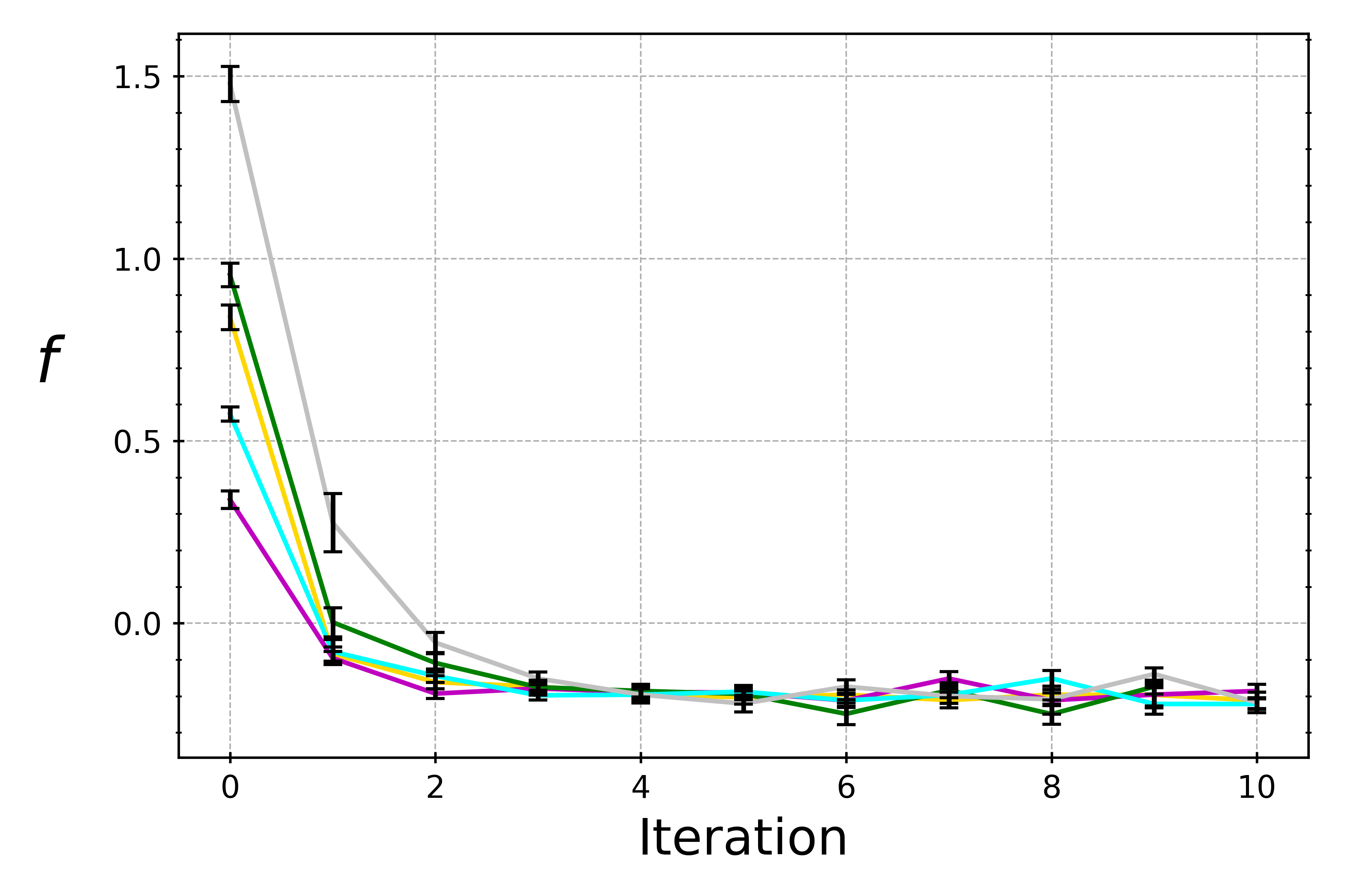
Five initial starting points were selected: = , , , . Optimization targeted the “true” interaction strength parameters: , , and , with an acceptable average relative deviation of 0.2 (refer to Figure 6). Twenty-five independent optimizations were performed per starting point, using 32 BICePs replicas and 200k MCMC steps per iteration.
For these tests, we required that the convergence condition must be satisfied two times in succession, which is a typical stopping point. Traces of the relative error throughout the optimization show a heterogeneous collection of convergence trajectories, depending on the starting point (Figure 6). At each iteration, we track the percentage of traces that remain unconverged. For some starting points, all optimization trajectories converge within ten iterations, while for others, up to 28% remain unconverged going into the tenth iteration. The average optimized parameters from the converged trajectories were determined to be , where the uncertainties are calculated from the inverse Hessian. An overlay of average traces on the BICePs score landscape is shown in Figure S13.
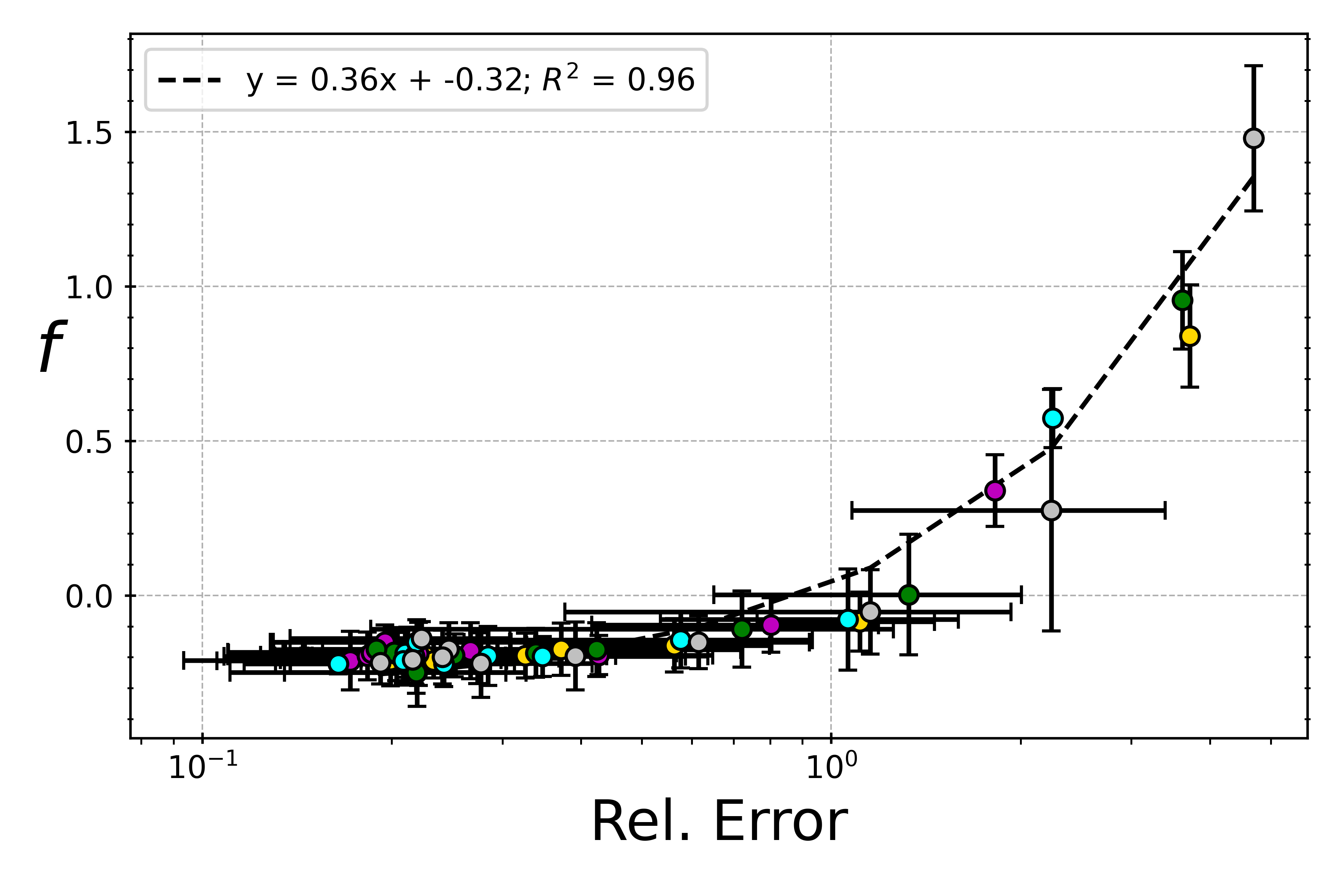
A robust correlation () between the converged BICePs score and the relative error in the parameters further confirms the validity of our approach in higher dimensions (see Figure S14). This relationship illustrates that an increased distance from the “true” parameters (i.e. a higher relative error) corresponds to an enlargement of the BICePs score . A comparative analysis of average BICePs scores across optimization traces (Figure S15) and the landscape contours (Figure S13) indicates that our Gaussian process regression does a fine job of approximating the actual BICePs score landscape in higher dimensions.

IV.7 Köfinger & Hummer’s toy polymer model
Köfinger and Hummer (KH) recently developed a method to optimize molecular simulation force fields using a Bayesian inference maximum-entropy reweighting method called BioFF.Köfinger and Hummer (2021) To validate their method, they introduced a simple parameterizable 2-D polymer model, and demonstrated that BioFF can efficiently discover the optimal parameters that reproduce ensemble-averaged observables. Here, we demonstrate that BICePs optimization can also reproduce this result.
The KH polymer model is a chain of beads, each separated by unit length, with orientations defined by angles between contiguous bond vectors. Each bond angle is distributed according a von Mises distribution parameterized by , which controls the polymer’s stiffness. Full details about this model are given in Appendix B. Unlike the HP lattice model, which possesses an exact solution for the prior, the KH polymer model requires estimation of the prior through statistical sampling, which is subject to finite sampling error.
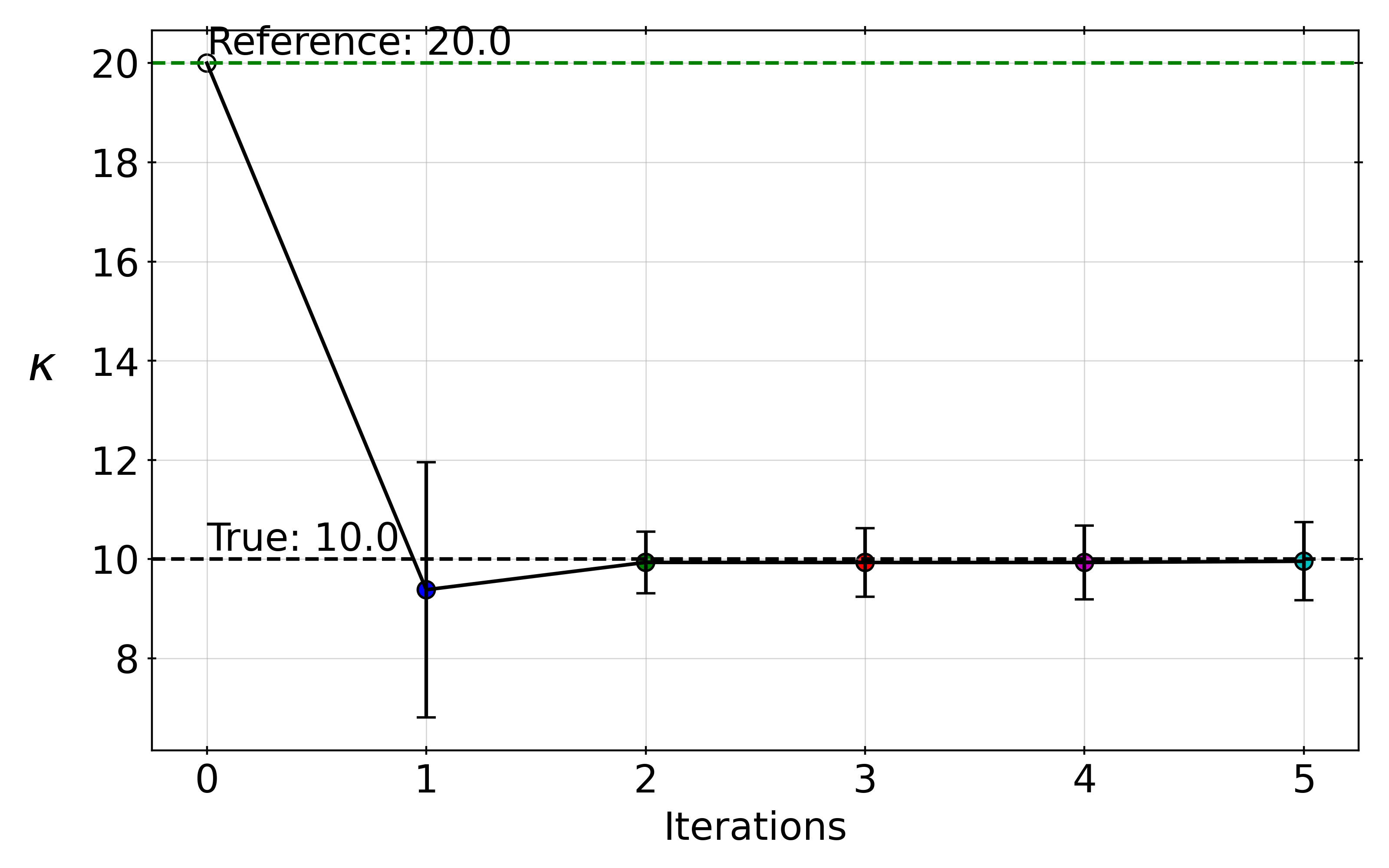
To implement KH model optimization with BICePs, we derived the first and second partial derivatives of the energy function required for computation of the BICePs score (see SI). Following Köfinger and Hummer, we consider a 100-bead chain, and use the end-to-middle distance (between bead 1 and bead 50) as the ensemble-averaged observable, which we estimate as the mean of 10000 samples from the von Mises distribution with the “true” value of set to 10.0.
We then performed ‘trust-ncg’ optimization using 200 BICePs replicas and 100k MCMC steps, starting from an initial parameter value of = 20.0. At the first optimization step, draw 500 samples from the von Mises distribution, and use their energies to compute their Boltzmann populations; each sample is a separate conformational state. In each subsequent optimization step, we draw 500 more samples to add to the collection, and compute energies and Boltzmann populations for the combined collection. The result of this procedure is highly efficient discovery of the optimal value of = 10, reaching convergence within two iterations (Figure S16).
While BICePs optimization achieves similar results to BioFF, it is worth mentioning some of the key differences of the two methods. BioFF is a maximum-entropy method that reweights a set of reference populations by minimizing a negative log-likelihood that uses a regularization parameter, , to balance two terms: the relative entropy with respect to the reference, and a term representing the deviation between model predictions of ensemble-averaged quantities and experiment. The BioFF-based optimization algorithm iteratively (1) reweights the populations given a current set of force field parameters, then (2) optimizes the force field parameters given the updated populations, repeating this cycle until convergence.
One issue with this approach is that it requires a coarse-grained description of the relevant conformational states and their populations, which need to be revised as the force field parameters are optimized. Köfinger and Hummer deal with this by keeping track of each new thermodynamic ensemble being sampled, and using the running collection of all the samples obtained to estimate each new set of coarse-grained state populations with the binless WHAMShirts and Chodera (2008); Rosta et al. (2011) free energy estimator. In our BICePs approach, we avoid this expense by simply adding new samples as additional conformational states, and recalculating populations as their Boltzmann weights.
Another issue with maximum-entropy methods like BioFFKöfinger, Różycki, and Hummer (2019); Köfinger and Hummer (2021) and BioEnBottaro, Bengtsen, and Lindorff-Larsen (2020) is the need to choose an appropriate value for the regularization parameter . BICePs does not require a regulation parameter, because the BICePs score is computed by sampling the entire posterior distribution of uncertainty parameters . (In BICePs, the are the analogous quantities that balance prior information against the experimental restraints.)
Very recently, Köfinger & Hummer put the regularization parameter on a firmer theoretical footing by relating it to the variance of the reduced energy difference, thus enabling estimation of a priori.Köfinger and Hummer (2023). Another recent work, Gilardoni et al. Gilardoni, Fröhlking, and Bussi (2023) introduced an approach similar to BICePs, in that ensemble refinement and force field parameter refinement are integrated into a singular process. This method bears resemblance to both BioEn and BioFF, as it employs a regularization parameter to scale the Kullback-Leibler divergence. Gilardoni et al.’s technique is distinguished by the incorporation of two distinct confidence hyperparameters. The first parameter is designed to adjust the reliability of the prior, while the second modulates the trustworthiness of the force field corrections.
IV.8 Further Discussion
Our work here greatly improves upon previous work by Ge et al., which used an HP lattice model as an example system to perform force field parameterization and model selection using BICePs.Ge and Voelz (2018). That work approached the problem through brute force, scanning parameter space in search of the minimum BICePs score, which would be costly and impractical for multiple parameters. Another issue with that work was the use of a previous version of BICePs (called BICePs v1.0) that does not use replica-averaging, and therefore was not a maximum-entropy method. Because of this, applying BICePs in practical cases, such as refining conformational populations against NMR observables for beta-hairpins trploop 2A and 2B, resulted in ensembles dominated by the state(s) that best agree with experiment. Since that work, we have developed the current version of BICePs that performs replica averaging and is equipped with specialized likelihood functions that can account for systematic error.Raddi, Ge, and Voelz (2023) The HP lattice model continues to serve as an excellent test system for force field refinement as it grants the option to use multiple parameters and provides exact solutions for generated ensembles.
While our algorithm has the advantage of being able to incorporate priors on force field parameters, this is a possibility we do not pursue in this work. Obtaining priors for force field parameters is a more involved approach, but we leave room for this in future development.
IV.9 Optimization across multiple systems
An eventual application of our BICePs optimization method is transferable force field parameterization across many different molecular systems (e.g. a set of proteins) against ensemble-averaged experimental measurements.
Our approach can easily be adapted for this purpose, and performed efficiently so that each molecular system can be evaluated in a separate BICePs calculation. To do this, suppose we have a set of molecular systems indexed by , of total number . We make use of the partial derivatives of the BICePs score with respect to each to determine a weight for each system . The normalized weight for the parameter of system is
| (22) |
At each optimization iteration, we update the parameter, according to a weighted average across all of the systems:
| (23) |
In this scheme, the derivatives play a pivotal role, where the weights are determined by how significantly each parameter change influences the BICePs score. This provides a balance, ensuring parameters from a system with larger effects on the score have more influence in determining the next set of parameters .
IV.10 Outlook
Looking ahead, there is tremendous potential to extend the scope of the BICePs optimization against ensemble averaged observables to many applications. One area of application would be to optimize physics-based molecular mechanics force fields for proteins against the many published solution-NMR data that exists.Cavender et al. (2023) Another application would be to optimize parameters of general-purpose force fields for bespoke applications. Examples of this may include refining existing all-atom microscopic models to better predict macroscopic properties (e.g. ensemble-average properties of disordered peptides like radius of gyration), or developing classes of models that can better predict the experimental observables for peptidomimetics without having to perform expensive fitting to quantum mechanical energy surfaces. In principle, any parameterizable model for the prior can be used with BICePs, including neural-network based potentials, or even generative models obtained from deep learning methods.
V Conclusion
In this work, we showed how the BICePs approach can be used for automatic and robust optimization of force field parameters against ensemble-averaged experimental measurements. This is done by variational minimization of the BICePs score, a free energy-like quantity characterizing how well a model agrees with the experimental data, calculated by sampling over the posterior distribution of possible uncertainties. Using information from first and second partial derivatives of the BICePs score with respect to model parameters, we show how robust multi-parameter optimization of the BICePs score can be performed. Demonstrations in simple toy protein lattice models and polymer models show the utility of the method, and how specialized likelihood functions to deal with outliers are especially good at dealing systematic error. These results suggest automated variational optimization of the BICePs score is a powerful approach for the parameterization of molecular potentials.
Conflicts of interest
Authors declare no conflicts of interest.
Data and software
The BICePs algorithm is freely available at github.com/vvoelz/biceps and can be installed using pip install biceps. The HP lattice model is open source software, located at:
github.com/vvoelz/HPSandbox. All data, scripts, Jupyter notebook examples and analysis can be found here: github.com/robraddi/biceps_FFOpt. Detailed documentation and tutorials can be found here: https://biceps. readthedocs.io. For any issues or questions, please submit the request on GitHub.
Acknowledgements
RMR and VAV are supported by National Institutes of Health grant R01GM123296.
References
- Boothroyd et al. (2023) S. Boothroyd, P. K. Behara, O. C. Madin, D. F. Hahn, H. Jang, V. Gapsys, J. R. Wagner, J. T. Horton, D. L. Dotson, M. W. Thompson, et al., “Development and benchmarking of open force field 2.0. 0: The sage small molecule force field,” Journal of Chemical Theory and Computation (2023).
- Smith et al. (2019) J. S. Smith, B. T. Nebgen, R. Zubatyuk, N. Lubbers, C. Devereux, K. Barros, S. Tretiak, O. Isayev, and A. E. Roitberg, “Approaching coupled cluster accuracy with a general-purpose neural network potential through transfer learning,” Nature communications 10, 2903 (2019).
- Köfinger and Hummer (2021) J. Köfinger and G. Hummer, “Empirical Optimization of Molecular Simulation Force Fields by Bayesian Inference,” The European Physical Journal B 94, 245 (2021).
- Wang, Martinez, and Pande (2014) L.-P. Wang, T. J. Martinez, and V. S. Pande, “Building Force Fields: An Automatic, Systematic, and Reproducible Approach,” The journal of physical chemistry letters 5, 1885–1891 (2014).
- Ge and Voelz (2018) Y. Ge and V. A. Voelz, “Model Selection Using BICePs: a Bayesian Approach for Force Field Validation and Parameterization,” J. Phys. Chem. B 122, 5610–5622 (2018).
- Madin et al. (2022) O. C. Madin, S. Boothroyd, R. A. Messerly, J. Fass, J. D. Chodera, and M. R. Shirts, “Bayesian-Inference-Driven Model Parametrization and Model Selection for 2CLJQ Fluid Models,” J. Chem. Inf. Model. 62, 874–889 (2022).
- Voelz, Ge, and Raddi (2021) V. A. Voelz, Y. Ge, and R. M. Raddi, “Reconciling Simulations and Experiments with BICePs: a Review,” Front. Mol. Biosci. 8, 661520 (2021).
- Raddi et al. (2023) R. M. Raddi, T. Marshall, Y. Ge, and V. Voelz, “Model Selection Using Replica Averaging with Bayesian Inference of Conformational Populations,” (2023).
- Voelz and Zhou (2014) V. a. Voelz and G. Zhou, “Bayesian Inference of Conformational State Populations from Computational Models and Sparse Experimental Observables,” J. Comput. Chem. 35, 2215–2224 (2014).
- Wan et al. (2020) H. Wan, Y. Ge, A. Razavi, and V. A. Voelz, “Reconciling Simulated Ensembles of Apomyoglobin with Experimental Hydrogen/Deuterium Exchange Data Using Bayesian Inference and Multiensemble Markov State Models.” J. Chem. Theory Comput. 16, 1333–1348 (2020).
- Hurley et al. (2021) M. F. D. Hurley, J. D. Northrup, Y. Ge, C. E. Schafmeister, and V. A. Voelz, “Metal Cation-Binding Mechanisms of Q-Proline Peptoid Macrocycles in Solution,” J. Chem. Inf. Model. 61, 2818–2828 (2021).
- Raddi, Ge, and Voelz (2023) R. M. Raddi, Y. Ge, and V. A. Voelz, “BICePs V2. 0: Software for Ensemble Reweighting Using Bayesian Inference of Conformational Populations,” Journal of chemical information and modeling 63, 2370–2381 (2023).
- Pitera and Chodera (2012) J. W. Pitera and J. D. Chodera, “On the Use of Experimental Observations to Bias Simulated Ensembles,” Journal of chemical theory and computation 8, 3445–3451 (2012).
- Cavalli, Camilloni, and Vendruscolo (2013) A. Cavalli, C. Camilloni, and M. Vendruscolo, “Molecular Dynamics Simulations with Replica-Averaged Structural Restraints Generate Structural Ensembles According to the Maximum Entropy Principle,” The Journal of chemical physics 138, 03B603 (2013).
- Cesari, Reißer, and Bussi (2018) A. Cesari, S. Reißer, and G. Bussi, “Using the Maximum Entropy Principle to Combine Simulations and Solution Experiments,” Computation 6, 15 (2018).
- Roux and Weare (2013) B. Roux and J. Weare, “On the Statistical Equivalence of Restrained-Ensemble Simulations with the Maximum Entropy Method,” The Journal of chemical physics 138, 02B616 (2013).
- Hummer and Köfinger (2015) G. Hummer and J. Köfinger, “Bayesian Ensemble Refinement by Replica Simulations and Reweighting,” The Journal of chemical physics 143, 12B634_1 (2015).
- Bonomi et al. (2016) M. Bonomi, C. Camilloni, A. Cavalli, and M. Vendruscolo, “Metainference: A Bayesian Inference Method for Heterogeneous Systems,” Sci. Adv. 2, e1501177 (2016).
- Sivia and Skilling (2006) D. Sivia and J. Skilling, Data Analysis: a Bayesian Tutorial (OUP Oxford, 2006).
- Dill et al. (1995) K. A. Dill, S. Bromberg, K. Yue, H. S. Chan, K. M. Ftebig, D. P. Yee, and P. D. Thomas, “Principles of protein folding—a perspective from simple exact models,” Protein science 4, 561–602 (1995).
- Byrd et al. (1995) R. H. Byrd, P. Lu, J. Nocedal, and C. Zhu, “A limited memory algorithm for bound constrained optimization,” SIAM Journal on scientific computing 16, 1190–1208 (1995).
- Wright (2006) S. J. Wright, Numerical optimization (2006).
- Beiranvand, Hare, and Lucet (2017) V. Beiranvand, W. Hare, and Y. Lucet, “Best Practices for Comparing Optimization Algorithms,” Optim. Eng. 18, 815–848 (2017).
- Shirts and Chodera (2008) M. R. Shirts and J. D. Chodera, “Statistically Optimal Analysis of Samples from Multiple Equilibrium States,” J. Chem. Phys. 129, 124105–11 (2008).
- Rosta et al. (2011) E. Rosta, M. Nowotny, W. Yang, and G. Hummer, “Catalytic mechanism of rna backbone cleavage by ribonuclease h from quantum mechanics/molecular mechanics simulations,” Journal of the American Chemical Society 133, 8934–8941 (2011).
- Köfinger, Różycki, and Hummer (2019) J. Köfinger, B. Różycki, and G. Hummer, “Inferring Structural Ensembles of Flexible and Dynamic Macromolecules Using Bayesian, Maximum Entropy, and Minimal-Ensemble Refinement Methods,” Biomolecular Simulations: Methods and Protocols , 341–352 (2019).
- Bottaro, Bengtsen, and Lindorff-Larsen (2020) S. Bottaro, T. Bengtsen, and K. Lindorff-Larsen, “Integrating Molecular Simulation and Experimental Data: a Bayesian/Maximum Entropy Reweighting Approach,” in Structural Bioinformatics (Springer, 2020) pp. 219–240.
- Köfinger and Hummer (2023) J. Köfinger and G. Hummer, “Encoding prior knowledge in ensemble refinement,” (2023).
- Gilardoni, Fröhlking, and Bussi (2023) I. Gilardoni, T. Fröhlking, and G. Bussi, “Boosting ensemble refinement with transferable force field corrections: synergistic optimization for molecular simulations,” arXiv preprint arXiv:2311.13532 (2023).
- Cavender et al. (2023) C. E. Cavender, D. A. Case, J. C.-H. Chen, L. T. Chong, D. A. Keedy, K. Lindorff-Larsen, D. L. Mobley, O. Ollila, C. Oostenbrink, P. Robustelli, V. A. Voelz, M. E. Wall, D. C. Wych, and M. K. Gilson, “Structure-based experimental datasets for benchmarking of protein simulation force fields,” arXiv preprint arXiv:2303.11056 (2023).
Appendix A Deriving the first and second derivatives of the BICePs score.
The BICePs score is defined as the negative logarithm of the Bayes factor, which is the quotient of two model evidences:
| (24) |
where the evidence for model with force field parameters is
| (25) |
and is the model evidence for the reference distribution, which is set to be a uniform ensemble (see Figure 1) and so, does not depend on . The partial derivatives of the BICePs score, , with respect to the model parameters , is:
| (26) |
where
| (27) |
This allows us to express the derivative of the BICePs score with respect to the force field parameter as:
| (28) |
which is the difference of Boltzmann averaged values of . This can also be explained in terms of prior energies. BICePs uses to scale the prior energies, where the reference ensemble is given . Therefore, the average energy of the reference ensemble is zero and
| (29) |
The Hessian matrix and corresponding second partial derivatives of the BICePs score is required for computing uncertainties of the inferred parameters by the covariance matrix (see equation 20), and when using a trust-region methods for optimization (see methods like ‘trust-ncg‘, ‘trust-exact‘ in ‘scipy.optimize.minimize‘). Trust-region methods can be more robust for noisy gradients; they may perform better with noisy objective functions because it does not rely solely on the gradient information to determine the search direction. Instead, it uses a combination of the gradient and second-order information with the local quadratic model to estimate the direction of steepest descent. The Hessian matrix contains elements of second-order partial derivatives with respect to each parameter and gives the curvature of the objective function.
| (30) |
The second-order partial derivative of the BICePs score for parameters and , where is given as
| (31) |
where
| (32) |
Putting this altogether and solving for equation 31 gives
| (33) |
which reduces to
| (34) | ||||
where the notation denotes the average with respect to . When (diagonal elements of the Hessian), the second-order partial derivatives of the BICePs score can be seen as the difference of the Boltzmann-averaged second-order partial derivative of the energy and the variance in its first-order partial derivative:
| (35) |
To compute the derivatives of the BICePs score, we need the first and second derivatives of the BICePs energy function , which consists of taking derivatives of the negative logarithm of the posterior, since . The derivative of this function with respect to some force field parameter is
| (36) |
The second derivative is
| (37) |
which can be reduced to
| (38) |
and when , the second-order partial derivative of the energy function becomes
| (39) |
Appendix B Kofinger & Hummer’s toy polymer model
As mentioned in the main text, the two dimensional polymer modelKöfinger and Hummer (2021) consists of a string of beads separated by a unit of length, where is the angle between the two bond vectors and . The associated probability of a polymer with beads is given by
| (40) |
where is the modified Bessel function of order zero and introduces directional biases. The parameters determine the stiffness of the polymer at positions . Prior energy, of the polymer configuration follow the Boltzmann distribution, which corresponds to
| (41) |
The authors did not provide derivatives of the toy model energy function, so we will briefly derive derivatives of the prior energies that will be used in our algorithm. The first derivative of the prior energy with respect to is
| (42) |
where the derivative of the von Mises distribution with respect to is
| (43) |
which is relatively straightforward since the derivative of the modified Bessel function merely increases it’s order. Next, the second derivative of with respect to :
| (44) |
where the second derivative of the von Mises distribution w.r.t is
| (45) | ||||
Appendix C Supplemental Information