A Novel Multivariate Skew-Normal Mixture Model and Its Application in Path-Planning for Very-Large-Scale Robotic Systems

Pingping Zhu1, Chang Liu2 and Peter Estephan3 *This research was made possible by the NASA Established Program to Stimulate Competitive Research, Grant # 80NSSC22M0027 and John Marshall University Scholars Awards1Pingping Zhu is with Faculty of Computer Sciences and Electrical Engineering, Marshall University, Huntington, WV, USA zhup@marshall.edu2Chang Liu is with the Department of Advanced Manufacturing and Robotics, College of Engineering, Peking University, Beijing 100871, China changliucoe@pku.edu.cn3Peter Estephan with the Department of Computer Sciences and Electrical Engineering, Marshall University, Huntington, WV, USA estephan@marshall.edu
Abstract

This paper addresses the path-planning challenge for very large-scale robotic systems (VLSR) operating in complex and cluttered environments. VLSR systems consist of numerous cooperative agents or robots working together autonomously. Traditionally, many approaches for VLSR systems are developed based on Gaussian mixture models (GMMs), where the GMMs represent agents’ evolving spatial distribution, serving as a macroscopic view of the system’s state. However, our recent research into VLSR systems has unveiled limitations in using GMMs to represent agent distributions, especially in cluttered environments. To overcome these limitations, we propose a novel model called the skew-normal mixture model (SNMM) for representing agent distributions. Additionally, we present a parameter learning algorithm designed to estimate the SNMM’s parameters using sample data. Furthermore, we develop two SNMM-based path-planning algorithms to guide VLSR systems through complex and cluttered environments. Our simulation results demonstrate the effectiveness and superiority of these algorithms compared to GMM-based path-planning methods.

I INTRODUCTION

With rapid advancements in computing and sensor technology, there is a growing interest in very-large-scale robotic (VLSR) systems. These systems, composed of numerous cooperative robots, offer significant advantages over single or small groups of robots, especially when they collaborate on common tasks through information sharing [1, 2, 3].

Various intelligent control approaches have emerged to understand and control the collective behavior of VLSR systems, particularly in scenarios like guiding or tracking robotic swarms through obstacle-filled environments. Because the optimal planning for cooperative robots is PSPACE-hard [4], the scalability issue is challenging for the VLSR problems. One promising approach is distributed optimal control (DOC) [5, 6, 7, 8], which uses time-varying probability density functions (PDFs) of robots or agents to represent the system’s macroscopic states. These PDFs guide the microscopic control of robots, addressing scalability challenges in VLSR systems. The Gaussian mixture model (GMM) is often used to model macroscopic states due to its simplicity and representation capabilities. However, recent research has revealed GMM’s limitations, especially in cluttered environments with many small-scale obstacles, such as forests [9]. This limitation of the GMM arises from its components, Gaussian or normal distributions, which are widely used in scientific and engineering areas due to their simple mathematical expression. However, Gaussian distributions’ simplicity reduces their flexibility and adaptability in representing robot distributions against complex environments, especially the cluttered environments. A large number of Gaussian components are required to construct a GMM to obtain an acceptable distribution representation performance, which violates the GMMs’ simplicity advantage.

This paper proposes novel statistical models based on multivariate skew-normal (SN) distributions to represent agent distributions in complex environments better. The univariate skew-normal family was formally defined by Azzalini in 1985 [10], and subsequent research introduced various definitions of multivariate skew-normal distributions [11, 12, 13]. These distributions share a crucial feature: their PDFs are proportional to the product of a Gaussian PDF and a skewing function, where the skewing function is typically a probability function or cumulative density function (CDF). Our approach considers interactions between agent distributions and obstacles, treating the obstacles’ occupancy probability function [14] as the skewing function. Additionally, we introduce the skew-normal mixture model (SNMM) to represent VLSR system macroscopic states, extending our skew-normal distributions. We also present a parameter learning algorithm to estimate SNMM parameters from agent positions. Simulation results demonstrate that this algorithm accurately estimates SNMM parameters, offering a superior macroscopic representation of agents with fewer components in cluttered, obstacle-filled environments than GMM. To showcase SNMM’s applications in VLSR systems, finally, we develop two SNMM-based path-planning algorithms for guiding large groups of agents through complex and cluttered environments, e.g., artificial forests. Simulations illustrate the effectiveness and superiority of these SNMM-based algorithms over GMM-based alternatives.

II MULTIVARIATE SKEW-NORMAL MIXTURE MODEL

A fundamental skew-normal (FUSN) distribution is defined in [13], and a modified version is provided as follows:

Definition 1 (Fundamental Skew-Normal Distribution)

Consider an nz×1subscript𝑛𝑧1n_{z}\times 1 random vector 𝐙nz𝐙superscriptsubscript𝑛𝑧\mathbf{Z}\in\mathbb{R}^{n_{z}}, and an nx×1subscript𝑛𝑥1n_{x}\times 1 random vector, 𝐗nx𝐗superscriptsubscript𝑛𝑥\mathbf{X}\in\mathbb{R}^{n_{x}}, where the random vector 𝐗𝐗\mathbf{X} is multivariate normal distributed, such that 𝐗𝒩(𝛍,𝚺)similar-to𝐗𝒩𝛍𝚺\mathbf{X}\sim\mathcal{N}(\boldsymbol{\mu},\boldsymbol{\Sigma}). The random variable, 𝐗=[𝐗|𝐙<𝛇]superscript𝐗delimited-[]conditional𝐗𝐙𝛇\mathbf{X}^{*}=\left[\mathbf{X}|\mathbf{Z}<\boldsymbol{\zeta}\right], is said to have a fundamental skew-normal (FUSN) distribution, denoted by 𝐗FUSN(𝛍,𝚺,Q𝐙)similar-tosuperscript𝐗𝐹𝑈𝑆𝑁𝛍𝚺subscript𝑄𝐙\mathbf{X}^{*}\sim FUSN(\boldsymbol{\mu},\boldsymbol{\Sigma},Q_{\mathbf{Z}}), if its PDF is given by

f𝐗(𝐱)=ϕ𝐗(𝐱|𝝁,𝚺)Q𝐙(𝐱)𝔼𝐗ϕ𝐗[Q𝐙(𝐗)]subscript𝑓superscript𝐗𝐱subscriptitalic-ϕ𝐗conditional𝐱𝝁𝚺subscript𝑄𝐙𝐱subscript𝔼similar-to𝐗subscriptitalic-ϕ𝐗delimited-[]subscript𝑄𝐙𝐗f_{\mathbf{X}^{*}}(\mathbf{x})=\frac{\phi_{\mathbf{X}}(\mathbf{x}|\boldsymbol{\mu},\boldsymbol{\Sigma})Q_{\mathbf{Z}}(\mathbf{x})}{\mathbb{E}_{\mathbf{X}\sim\phi_{\mathbf{X}}}[Q_{\mathbf{Z}}(\mathbf{X})]} (1)

where 𝛇nz𝛇superscriptsubscript𝑛𝑧\boldsymbol{\zeta}\in\mathbb{R}^{n_{z}} is a user-defined threshold vector, ϕ𝐗(𝐱|𝛍,𝚺)subscriptitalic-ϕ𝐗conditional𝐱𝛍𝚺\phi_{\mathbf{X}}(\mathbf{x}|\boldsymbol{\mu},\boldsymbol{\Sigma}) is the PDF of the multivariate normal random vector 𝐗𝐗\mathbf{X}, and Q𝐙(𝐱)P(𝐙<𝛇|𝐗=𝐱)subscript𝑄𝐙𝐱𝑃𝐙bra𝛇𝐗𝐱Q_{\mathbf{Z}}(\mathbf{x})\triangleq P(\mathbf{Z}<\boldsymbol{\zeta}|\mathbf{X}=\mathbf{x}).

Here, the function Q𝐙(𝐱)subscript𝑄𝐙𝐱Q_{\mathbf{Z}}(\mathbf{x}) is a skewing function, and 𝔼𝐗ϕ𝐗[]subscript𝔼similar-to𝐗subscriptitalic-ϕ𝐗delimited-[]\mathbb{E}_{\mathbf{X}\sim\phi_{\mathbf{X}}}[\cdot] denotes the expectation with respect to (w.r.t.) the PDF ϕ𝐗subscriptitalic-ϕ𝐗\phi_{\mathbf{X}}. According to [13], Definition 1 can contain many different families of skew-normal distributions. In this section, we propose a new skew-normal distribution based on Definition 1 by embedding the environmental information. Furthermore, a skew-normal mixture model (SNMM) is proposed to describe the statistics of VLSR systems in obstacle-deployed environments. Finally, a parameter learning algorithm is developed to estimate the model parameters of the SNMM from samples.

II-A Multivariate Skew-Normal Distribution

In the VLSR problems, the position of the n𝑛nth agent can be considered as a continuous random vector, 𝐗n𝒲subscript𝐗𝑛𝒲\mathbf{X}_{n}\in\mathcal{W}, n=1,,N𝑛1𝑁n=1,\ldots,N, where 𝒲2𝒲superscript2\mathcal{W}\subset\mathbb{R}^{2} denotes the workspace. If we assume that {𝐗n}n=1Nsuperscriptsubscriptsubscript𝐗𝑛𝑛1𝑁\{\mathbf{X}_{n}\}_{n=1}^{N} are all independent and identically distributed (i.i.d.) multivariate normal random vector denoted by 𝐗𝒩(𝝁,𝚺)similar-to𝐗𝒩𝝁𝚺\mathbf{X}\sim\mathcal{N}(\boldsymbol{\mu},\boldsymbol{\Sigma}), then the actual positions of N𝑁N agents can be treated as N𝑁N independent samples/realizations generated from 𝐗𝐗\mathbf{X}.

On the other hand, let 𝒲𝒲\mathcal{B}\subset\mathcal{W} denote the set of the locations occupied by obstacles in the workspace. We can have a Bernoulli random variable Y(𝐱){0,1}𝑌𝐱01Y(\mathbf{x})\in\{0,1\} indicating if the location 𝐱𝒲𝐱𝒲\mathbf{x}\in\mathcal{W} is occupied by the obstacles, such that Y(𝐱)=1𝑌𝐱1Y(\mathbf{x})=1 if 𝐱𝐱\mathbf{x}\in\mathcal{B}, otherwise, Y(𝐱)=0𝑌𝐱0Y(\mathbf{x})=0. Thus, Y(𝐗)𝑌𝐗Y(\mathbf{X}) defined on the whole workspace specifies a Bernoulli-random-field (BRF). Furthermore, consider the scenario where the obstacle detection can be determined via observing a continuous random measurement, 𝐙(𝐱)𝐙𝐱\mathbf{Z}(\mathbf{x}), obtained at 𝐱𝐱\mathbf{x}, such that P(Y(𝐱)=1)=P(𝐙(𝐱)𝜻)𝑃𝑌𝐱1𝑃𝐙𝐱𝜻P(Y(\mathbf{x})=1)=P(\mathbf{Z}(\mathbf{x})\geq\boldsymbol{\zeta}), where 𝜻𝜻\boldsymbol{\zeta} indicates a user-defined threshold parameter. Then, because the agents cannot be deployed on the obstacles, the distribution of the agents in an obstacle-deployed environment can be modeled by a FUSN distribution defined in Definition 1.

Finally, considering the direct interaction between agents and obstacles, we can construct a novel skew-normal distribution based on FUSN to describe the statistical model for the VLSR problem referred to as the Bernoulli-random-filed based skew-normal (BRF-SN) distribution, which is defined as follows.

Definition 2 (Bernoulli-Random-Field based Skew-Normal Distribution)

Consider a continuous random vector, 𝐗nx𝐗superscriptsubscript𝑛𝑥\mathbf{X}\in\mathbb{R}^{n_{x}} and a Bernoulli random variable Y{0,1}𝑌01Y\in\{0,1\}, where the random vector 𝐗𝐗\mathbf{X} is multivariate normal distributed, such that 𝐗𝒩(𝛍,𝚺)similar-to𝐗𝒩𝛍𝚺\mathbf{X}\sim\mathcal{N}(\boldsymbol{\mu},\boldsymbol{\Sigma}). The random variable, 𝐗=[𝐗|Y=0]superscript𝐗delimited-[]conditional𝐗𝑌0\mathbf{X}^{*}=\left[\mathbf{X}|Y=0\right], has a Bernoulli-random-field based skew-normal (BRF-SN) distribution denoted by 𝐗BRFSN(𝛍,𝚺,QY)similar-tosuperscript𝐗𝐵𝑅𝐹𝑆𝑁𝛍𝚺subscript𝑄𝑌\mathbf{X}^{*}\sim BRFSN(\boldsymbol{\mu},\boldsymbol{\Sigma},Q_{Y}), if its PDF is given by

f𝐗(𝐱)=ϕ𝐗(𝐱|𝝁,𝚺)QY(𝐱)𝔼𝐗ϕ𝐗[QY(𝐗)]subscript𝑓superscript𝐗𝐱subscriptitalic-ϕ𝐗conditional𝐱𝝁𝚺subscript𝑄𝑌𝐱subscript𝔼similar-to𝐗subscriptitalic-ϕ𝐗delimited-[]subscript𝑄𝑌𝐗f_{\mathbf{X}^{*}}(\mathbf{x})=\frac{\phi_{\mathbf{X}}(\mathbf{x}|\boldsymbol{\mu},\boldsymbol{\Sigma})Q_{Y}(\mathbf{x})}{\mathbb{E}_{\mathbf{X}\sim\phi_{\mathbf{X}}}[Q_{Y}(\mathbf{X})]} (2)

where ϕ𝐗(𝐱|𝛍,𝚺)subscriptitalic-ϕ𝐗conditional𝐱𝛍𝚺\phi_{\mathbf{X}}(\mathbf{x}|\boldsymbol{\mu},\boldsymbol{\Sigma}) is the PDF of the multivariate normal random vector 𝐗𝐗\mathbf{X}, and QY(𝐱)P(Y(𝐗)=0|𝐗=𝐱)subscript𝑄𝑌𝐱𝑃𝑌𝐗conditional0𝐗𝐱Q_{Y}(\mathbf{x})\triangleq P(Y(\mathbf{X})=0|\mathbf{X}=\mathbf{x}).

Notably, the skewing function, QY(𝐱)subscript𝑄𝑌𝐱Q_{Y}(\mathbf{x}), can be obtained through many approaches, e.g., the Hilbert occupancy map. The readers are referred to [14, 15, 16, 8].

II-B Skew-Normal Mixture Model

To describe a more complex agents’ distribution, we extended the BRF-SN distribution to a mixture model associated with the following PDF,

𝐗(𝐱)i=1NCωif𝐗,i(𝐱|𝝁i,𝚺i)subscriptWeierstrass-psuperscript𝐗𝐱superscriptsubscript𝑖1subscript𝑁𝐶subscript𝜔𝑖subscript𝑓superscript𝐗𝑖conditional𝐱subscript𝝁𝑖subscript𝚺𝑖\wp_{\mathbf{X}^{*}}(\mathbf{x})\triangleq\sum_{i=1}^{N_{C}}\omega_{i}f_{\mathbf{X}^{*},i}(\mathbf{x}|\boldsymbol{\mu}_{i},\boldsymbol{\Sigma}_{i}) (3)

This statistical model, referred to as the Bernoulli-random-field based skew-normal mixture model (BRF-SNMM), consists of NCsubscript𝑁𝐶N_{C} BRF-SN components, {f𝐗,i(𝐱|𝝁i,𝚺i)}i=1NCsuperscriptsubscriptsubscript𝑓superscript𝐗𝑖conditional𝐱subscript𝝁𝑖subscript𝚺𝑖𝑖1subscript𝑁𝐶\{f_{\mathbf{X}^{*},i}(\mathbf{x}|\boldsymbol{\mu}_{i},\boldsymbol{\Sigma}_{i})\}_{i=1}^{N_{C}}, defined in Definition 2 associated with the corresponding weights, {ωi}i=1NCsuperscriptsubscriptsubscript𝜔𝑖𝑖1subscript𝑁𝐶\{\omega_{i}\}_{i=1}^{N_{C}}. Given the skewing function QY(𝐱)subscript𝑄𝑌𝐱Q_{Y}(\mathbf{x}), therefore, the BRF-SNMM is specified by the component parameters 𝚯i=(𝝁i,𝚺i)subscript𝚯𝑖subscript𝝁𝑖subscript𝚺𝑖\boldsymbol{\Theta}_{i}=(\boldsymbol{\mu}_{i},\boldsymbol{\Sigma}_{i}), i=1,,NC𝑖1subscript𝑁𝐶i=1,\ldots,N_{C}, and the weight parameters, 𝝎=[ω1ωNC]𝝎matrixsubscript𝜔1subscript𝜔subscript𝑁𝐶\boldsymbol{\omega}=\begin{bmatrix}\omega_{1}&\ldots&\omega_{N_{C}}\end{bmatrix}, such that i=1NCωi=1superscriptsubscript𝑖1subscript𝑁𝐶subscript𝜔𝑖1\sum_{i=1}^{N_{C}}\omega_{i}=1 and ωi>0subscript𝜔𝑖0\omega_{i}>0 for all i𝑖i, which are also denoted by 𝚯1:NC={(ωi,𝚯i)}i=1NCsubscript𝚯:1subscript𝑁𝐶superscriptsubscriptsubscript𝜔𝑖subscript𝚯𝑖𝑖1subscript𝑁𝐶\boldsymbol{\Theta}_{1:N_{C}}=\{(\omega_{i},\boldsymbol{\Theta}_{i})\}_{i=1}^{N_{C}} for short.

II-C Parameters Learning For Skew-Normal Mixture Model

Because the BRF-SNMM has a structure similar to the GMM, we can also use the expectation-maximization (EM) method to learn the parameters from the given samples, 𝒟={𝐱n}n=1N𝒟superscriptsubscriptsubscript𝐱𝑛𝑛1𝑁\mathcal{D}=\{\mathbf{x}_{n}\}_{n=1}^{N}. First, we consider an NCsubscript𝑁𝐶N_{C}-dimensional categorical random variable, C{1,,NC}𝐶1subscript𝑁𝐶C\in\{1,\ldots,N_{C}\}, indicating the label of the BRF-SN components. Given the parameters, 𝚯1:NCsubscript𝚯:1subscript𝑁𝐶\boldsymbol{\Theta}_{1:N_{C}}, the conditional distribution can be specified by the component weight 𝝎𝝎\boldsymbol{\omega}, such that P(C=i|𝚯1:NC)=ωi, for i=1,,NCformulae-sequence𝑃𝐶conditional𝑖subscript𝚯:1subscript𝑁𝐶subscript𝜔𝑖 for 𝑖1subscript𝑁𝐶P(C=i|\boldsymbol{\Theta}_{1:N_{C}})=\omega_{i},\text{ for }i=1,\ldots,N_{C}. Thus, the BRF-SN distribution, f𝐗i(𝐱|𝝁i,𝚺i)subscript𝑓subscriptsuperscript𝐗𝑖conditional𝐱subscript𝝁𝑖subscript𝚺𝑖f_{\mathbf{X}^{*}_{i}}(\mathbf{x}|\boldsymbol{\mu}_{i},\boldsymbol{\Sigma}_{i}), can be interpreted as the conditional distribution of the random variable 𝐗superscript𝐗\mathbf{X}^{*}, given 𝐗superscript𝐗\mathbf{X}^{*} is associated with the i𝑖ith BRF-SN component, such that 𝐗|C(𝐱|C=i,𝚯1:NC)=f𝐗,i(𝐱|𝝁i,𝚺i)subscriptWeierstrass-pconditionalsuperscript𝐗𝐶conditional𝐱𝐶𝑖subscript𝚯:1subscript𝑁𝐶subscript𝑓superscript𝐗𝑖conditional𝐱subscript𝝁𝑖subscript𝚺𝑖\wp_{\mathbf{X}^{*}|C}(\mathbf{x}|C=i,\boldsymbol{\Theta}_{1:N_{C}})=f_{\mathbf{X}^{*},i}(\mathbf{x}|\boldsymbol{\mu}_{i},\boldsymbol{\Sigma}_{i}).

To specify the unknown underlying parameters, 𝚯1:NCsubscript𝚯:1subscript𝑁𝐶\boldsymbol{\Theta}_{1:N_{C}}, from the samples, we can construct the following negative loglikelihood (NLL) object function,

J(𝚯1:NC|𝒟)n=1N(𝐱n,𝚯1:NC)𝐽conditionalsubscript𝚯:1subscript𝑁𝐶𝒟superscriptsubscript𝑛1𝑁subscript𝐱𝑛subscript𝚯:1subscript𝑁𝐶J(\boldsymbol{\Theta}_{1:N_{C}}|\mathcal{D})\triangleq\sum_{n=1}^{N}\mathcal{L}(\mathbf{x}_{n},\boldsymbol{\Theta}_{1:N_{C}}) (4)

where the term, (𝐱n,𝚯1:NC)subscript𝐱𝑛subscript𝚯:1subscript𝑁𝐶\mathcal{L}(\mathbf{x}_{n},\boldsymbol{\Theta}_{1:N_{C}}), is defined by

(𝐱n,𝚯1:NC)subscript𝐱𝑛subscript𝚯:1subscript𝑁𝐶\displaystyle\mathcal{L}(\mathbf{x}_{n},\boldsymbol{\Theta}_{1:N_{C}}) ln[𝐗(𝐱n|𝚯1:NC)]absentsubscriptWeierstrass-psuperscript𝐗conditionalsubscript𝐱𝑛subscript𝚯:1subscript𝑁𝐶\displaystyle\triangleq-\ln\bigg{[}\wp_{\mathbf{X}^{*}}(\mathbf{x}_{n}|\boldsymbol{\Theta}_{1:N_{C}})\bigg{]} (5)
=ln𝔼C|𝐱n[𝐗,C(𝐱n,C=i|𝚯1:NC)P(C=i|𝐱n)]absentsubscript𝔼conditional𝐶subscript𝐱𝑛delimited-[]subscriptWeierstrass-psuperscript𝐗𝐶subscript𝐱𝑛𝐶conditional𝑖subscript𝚯:1subscript𝑁𝐶𝑃𝐶conditional𝑖subscript𝐱𝑛\displaystyle=-\ln\mathbb{E}_{C|\mathbf{x}_{n}}\bigg{[}\frac{\wp_{\mathbf{X}^{*},C}(\mathbf{x}_{n},C=i|\boldsymbol{\Theta}_{1:N_{C}})}{P(C=i|\mathbf{x}_{n})}\bigg{]}

Here, 𝔼C|𝐱n[]subscript𝔼conditional𝐶subscript𝐱𝑛delimited-[]\mathbb{E}_{C|\mathbf{x}_{n}}[\cdot] indicates the expectation term w.r.t. the discrete distribution P(C|𝐱n)𝑃conditional𝐶subscript𝐱𝑛P(C|\mathbf{x}_{n}).

Similar to the GMM parameter learning approach, a upper bound of the NLL object function is provided as follows,

J~(𝚪,𝚯1:NC|𝒟)n=1N~(𝐱n,𝜸n,𝚯1:NC)~𝐽𝚪conditionalsubscript𝚯:1subscript𝑁𝐶𝒟superscriptsubscript𝑛1𝑁~subscript𝐱𝑛subscript𝜸𝑛subscript𝚯:1subscript𝑁𝐶\tilde{J}(\boldsymbol{\Gamma},\boldsymbol{\Theta}_{1:N_{C}}|\mathcal{D})\triangleq\sum_{n=1}^{N}\tilde{\mathcal{L}}(\mathbf{x}_{n},\boldsymbol{\gamma}_{n},\boldsymbol{\Theta}_{1:N_{C}}) (6)

where γn,iC|𝐗(C=i|𝐱n,𝚯1:NC)subscript𝛾𝑛𝑖subscriptWeierstrass-pconditional𝐶superscript𝐗𝐶conditional𝑖subscript𝐱𝑛subscript𝚯:1subscript𝑁𝐶\gamma_{n,i}\triangleq\wp_{C|\mathbf{X}^{*}}(C=i|\mathbf{x}_{n},\boldsymbol{\Theta}_{1:N_{C}}), 𝜸n=[γn,1γn,NC]=C|𝐗(C|𝐱n,𝚯1:NC)subscript𝜸𝑛matrixsubscript𝛾𝑛1subscript𝛾𝑛subscript𝑁𝐶subscriptWeierstrass-pconditional𝐶superscript𝐗conditional𝐶subscript𝐱𝑛subscript𝚯:1subscript𝑁𝐶\boldsymbol{\gamma}_{n}=\begin{bmatrix}\gamma_{n,1}&\ldots&\gamma_{n,N_{C}}\end{bmatrix}=\wp_{C|\mathbf{X}^{*}}(C|\mathbf{x}_{n},\boldsymbol{\Theta}_{1:N_{C}}), and 𝚪=[γn,i]n=1,i=1N,NC𝚪superscriptsubscriptmatrixsubscript𝛾𝑛𝑖formulae-sequence𝑛1𝑖1𝑁subscript𝑁𝐶\boldsymbol{\Gamma}=\begin{bmatrix}\gamma_{n,i}\end{bmatrix}_{n=1,i=1}^{N,N_{C}} is a N×NC𝑁subscript𝑁𝐶N\times N_{C} matrix. Here, the term ~(𝐱n,𝜸n,𝚯1:NC)~subscript𝐱𝑛subscript𝜸𝑛subscript𝚯:1subscript𝑁𝐶\tilde{\mathcal{L}}(\mathbf{x}_{n},\boldsymbol{\gamma}_{n},\boldsymbol{\Theta}_{1:N_{C}}) is a tight upper bound of (𝐱n,𝚯1:NC)subscript𝐱𝑛subscript𝚯:1subscript𝑁𝐶\mathcal{L}(\mathbf{x}_{n},\boldsymbol{\Theta}_{1:N_{C}}), which is defined by

~(𝐱n,𝜸n,𝚯1:NC)~subscript𝐱𝑛subscript𝜸𝑛subscript𝚯:1subscript𝑁𝐶\displaystyle\tilde{\mathcal{L}}(\mathbf{x}_{n},\boldsymbol{\gamma}_{n},\boldsymbol{\Theta}_{1:N_{C}}) i=1NCγn,iln[γn,i𝐗,C(𝐱n,C=i|𝚯1:NC)]absentsuperscriptsubscript𝑖1subscript𝑁𝐶subscript𝛾𝑛𝑖subscript𝛾𝑛𝑖subscriptWeierstrass-psuperscript𝐗𝐶subscript𝐱𝑛𝐶conditional𝑖subscript𝚯:1subscript𝑁𝐶\displaystyle\triangleq\sum_{i=1}^{N_{C}}\gamma_{n,i}\ln\bigg{[}\frac{\gamma_{n,i}}{\wp_{\mathbf{X}^{*},C}(\mathbf{x}_{n},C=i|\boldsymbol{\Theta}_{1:N_{C}})}\bigg{]}
=i=1NCγn,iln[γn,iωif𝐗,i(𝐱|𝝁i,𝚺i)]absentsuperscriptsubscript𝑖1subscript𝑁𝐶subscript𝛾𝑛𝑖subscript𝛾𝑛𝑖subscript𝜔𝑖subscript𝑓superscript𝐗𝑖conditional𝐱subscript𝝁𝑖subscript𝚺𝑖\displaystyle=\sum_{i=1}^{N_{C}}\gamma_{n,i}\ln\bigg{[}\frac{\gamma_{n,i}}{\omega_{i}f_{\mathbf{X}^{*},i}(\mathbf{x}|\boldsymbol{\mu}_{i},\boldsymbol{\Sigma}_{i})}\bigg{]} (7)

The upper bound, ~(𝐱n,𝜸n,𝚯1:NC)~subscript𝐱𝑛subscript𝜸𝑛subscript𝚯:1subscript𝑁𝐶\tilde{\mathcal{L}}(\mathbf{x}_{n},\boldsymbol{\gamma}_{n},\boldsymbol{\Theta}_{1:N_{C}}), is obtained according to Jensen’s inequality [17]. The details are omitted because of limited pages.

Then, we apply the EM method to optimize the upper bound, J~(𝚪,𝚯1:NC)~𝐽𝚪subscript𝚯:1subscript𝑁𝐶\tilde{J}(\boldsymbol{\Gamma},\boldsymbol{\Theta}_{1:N_{C}}), including the expectation step (E-step) and the maximization step (M-step). In the E-step, we calculate the conditional distribution, C|𝐗(C=i|𝐱n,𝚯1:NC)subscriptWeierstrass-pconditional𝐶superscript𝐗𝐶conditional𝑖subscript𝐱𝑛superscriptsubscript𝚯:1subscript𝑁𝐶\wp_{C|\mathbf{X}^{*}}(C=i|\mathbf{x}_{n},\boldsymbol{\Theta}_{1:N_{C}}^{\ell}), for every sample, 𝐱nsubscript𝐱𝑛\mathbf{x}_{n}, given the parameter, 𝚯1:NCsuperscriptsubscript𝚯:1subscript𝑁𝐶\boldsymbol{\Theta}_{1:N_{C}}^{\ell}, obtained at the \ell iteration, such that

γn,isuperscriptsubscript𝛾𝑛𝑖\displaystyle\gamma_{n,i}^{\ell} =C|𝐗(C=i|𝐱n,𝚯1:NC)absentsubscriptWeierstrass-pconditional𝐶superscript𝐗𝐶conditional𝑖subscript𝐱𝑛superscriptsubscript𝚯:1subscript𝑁𝐶\displaystyle=\wp_{C|\mathbf{X}^{*}}(C=i|\mathbf{x}_{n},\boldsymbol{\Theta}_{1:N_{C}}^{\ell})
=ωif𝐗,i(𝐱n|𝝁i,𝚺i)i=1NCωif𝐗,i(𝐱n|𝝁i,𝚺i), for i=1,,NCformulae-sequenceabsentsuperscriptsubscript𝜔𝑖subscript𝑓superscript𝐗𝑖conditionalsubscript𝐱𝑛superscriptsubscript𝝁𝑖superscriptsubscript𝚺𝑖superscriptsubscript𝑖1subscript𝑁𝐶superscriptsubscript𝜔𝑖subscript𝑓superscript𝐗𝑖conditionalsubscript𝐱𝑛superscriptsubscript𝝁𝑖superscriptsubscript𝚺𝑖 for 𝑖1subscript𝑁𝐶\displaystyle=\frac{\omega_{i}^{\ell}f_{\mathbf{X}^{*},i}(\mathbf{x}_{n}|\boldsymbol{\mu}_{i}^{\ell},\boldsymbol{\Sigma}_{i}^{\ell})}{\sum_{i=1}^{N_{C}}\omega_{i}^{\ell}f_{\mathbf{X}^{*},i}(\mathbf{x}_{n}|\boldsymbol{\mu}_{i}^{\ell},\boldsymbol{\Sigma}_{i}^{\ell})},\text{ for }i=1,\ldots,N_{C} (8)

In the M-step, fixing 𝚪=[γn,i]n=1,i=1N,NCsuperscript𝚪superscriptsubscriptmatrixsuperscriptsubscript𝛾𝑛𝑖formulae-sequence𝑛1𝑖1𝑁subscript𝑁𝐶\boldsymbol{\Gamma}^{\ell}=\begin{bmatrix}\gamma_{n,i}^{\ell}\end{bmatrix}_{n=1,i=1}^{N,N_{C}} obtained in the E-step, we minimize J~(𝚪,𝚯1:NC)~𝐽superscript𝚪subscript𝚯:1subscript𝑁𝐶\tilde{J}(\boldsymbol{\Gamma}^{\ell},\boldsymbol{\Theta}_{1:N_{C}}) w.r.t. the parameters, 𝚯1:NCsubscript𝚯:1subscript𝑁𝐶\boldsymbol{\Theta}_{1:N_{C}}, for the (+1)1(\ell+1)th iteration, such that

𝚯1:NC+1=argmin𝚯1:NCJ~(𝚪,𝚯1:NC)superscriptsubscript𝚯:1subscript𝑁𝐶1subscript𝚯:1subscript𝑁𝐶~𝐽superscript𝚪subscript𝚯:1subscript𝑁𝐶\boldsymbol{\Theta}_{1:N_{C}}^{\ell+1}=\underset{\boldsymbol{\Theta}_{1:N_{C}}}{\arg\min}\tilde{J}(\boldsymbol{\Gamma}^{\ell},\boldsymbol{\Theta}_{1:N_{C}}) (9)

Considering that i=1NCωi=1superscriptsubscript𝑖1subscript𝑁𝐶subscript𝜔𝑖1\sum_{i=1}^{N_{C}}\omega_{i}=1 and ωi>0subscript𝜔𝑖0\omega_{i}>0 for all i𝑖i, 𝝎+1=[ω1+1ωNC+1]superscript𝝎1matrixsuperscriptsubscript𝜔11superscriptsubscript𝜔subscript𝑁𝐶1\boldsymbol{\omega}^{\ell+1}=\begin{bmatrix}\omega_{1}^{\ell+1}&\ldots&\omega_{N_{C}}^{\ell+1}\end{bmatrix} can be updated by

ωi+1=n=1Nγn,in=1Ni=1NCγn,i=n=1Nγn,iN for i=1,,NCformulae-sequencesuperscriptsubscript𝜔𝑖1superscriptsubscript𝑛1𝑁superscriptsubscript𝛾𝑛𝑖superscriptsubscript𝑛1𝑁superscriptsubscript𝑖1subscript𝑁𝐶superscriptsubscript𝛾𝑛𝑖superscriptsubscript𝑛1𝑁superscriptsubscript𝛾𝑛𝑖𝑁 for 𝑖1subscript𝑁𝐶\omega_{i}^{\ell+1}=\frac{\sum_{n=1}^{N}\gamma_{n,i}^{\ell}}{\sum_{n=1}^{N}\sum_{i=1}^{N_{C}}\gamma_{n,i}^{\ell}}=\frac{\sum_{n=1}^{N}\gamma_{n,i}^{\ell}}{N}\text{ for }i=1,\ldots,N_{C} (10)

Furthermore, we use the gradient-decent method to obtain the parameters, 𝚯i+1=(𝝁i+1,𝚺i+1)superscriptsubscript𝚯𝑖1superscriptsubscript𝝁𝑖1superscriptsubscript𝚺𝑖1\boldsymbol{\Theta}_{i}^{\ell+1}=(\boldsymbol{\mu}_{i}^{\ell+1},\boldsymbol{\Sigma}_{i}^{\ell+1}) by calculating the partial derivatives of J~(𝚪,𝚯1:NC)~𝐽superscript𝚪subscript𝚯:1subscript𝑁𝐶\tilde{J}(\boldsymbol{\Gamma}^{\ell},\boldsymbol{\Theta}_{1:N_{C}}) w.r.t. 𝝁isubscript𝝁𝑖\boldsymbol{\mu}_{i} and 𝚺isubscript𝚺𝑖\boldsymbol{\Sigma}_{i}, recursively, at the \ellth learning iteration. Considering the constraint that 𝚺i+1superscriptsubscript𝚺𝑖1\boldsymbol{\Sigma}_{i}^{\ell+1} must be a positive definite matrix, we update 𝚺i+1superscriptsubscript𝚺𝑖1\boldsymbol{\Sigma}_{i}^{\ell+1} using the partial derivative w.r.t. the matrix 𝐋isubscript𝐋𝑖\mathbf{L}_{i} instead of 𝚺isubscript𝚺𝑖\boldsymbol{\Sigma}_{i}, where

𝚺i1=𝐋i𝐋iTsuperscriptsubscript𝚺𝑖1subscript𝐋𝑖superscriptsubscript𝐋𝑖𝑇\boldsymbol{\Sigma}_{i}^{-1}=\mathbf{L}_{i}\mathbf{L}_{i}^{T} (11)

and the superscript “T𝑇T” indicates the transpose operation. Specifically, the derivatives of J~(𝚪,𝚯1:K)~𝐽superscript𝚪subscript𝚯:1𝐾\tilde{J}(\boldsymbol{\Gamma}^{\ell},\boldsymbol{\Theta}_{1:K}) w.r.t. 𝝁isubscript𝝁𝑖\boldsymbol{\mu}_{i} and 𝐋isubscript𝐋𝑖\mathbf{L}_{i} can be expressed by

J~𝝁i=ωi+1N𝚺i1[𝔼𝐗ϕ𝐗,i[𝐗QY(𝐗)]𝔼𝐗ϕ𝐗,i[QY(𝐗)]𝝁^i]~𝐽subscript𝝁𝑖superscriptsubscript𝜔𝑖1𝑁superscriptsubscript𝚺𝑖1delimited-[]subscript𝔼similar-to𝐗subscriptitalic-ϕ𝐗𝑖delimited-[]𝐗subscript𝑄𝑌𝐗subscript𝔼similar-to𝐗subscriptitalic-ϕ𝐗𝑖delimited-[]subscript𝑄𝑌𝐗subscript^𝝁𝑖\frac{\partial\tilde{J}}{\partial\boldsymbol{\mu}_{i}}=\omega_{i}^{\ell+1}N\boldsymbol{\Sigma}_{i}^{-1}\bigg{[}\frac{\mathbb{E}_{\mathbf{X}\sim\phi_{\mathbf{X},i}}[\mathbf{X}Q_{Y}(\mathbf{X})]}{\mathbb{E}_{\mathbf{X}\sim\phi_{\mathbf{X},i}}[Q_{Y}(\mathbf{X})]}-\hat{\boldsymbol{\mu}}_{i}\bigg{]} (12)
J~𝐋i=~𝐽subscript𝐋𝑖absent\displaystyle\frac{\partial\tilde{J}}{\partial\mathbf{L}_{i}}= ωi+1N{𝔼𝐗ϕ𝐗,i[(𝐗𝝁i)(𝐗𝝁i)TQY(𝐗)]𝔼𝐗ϕ𝐗,i[QY(𝐗)]\displaystyle-\omega_{i}^{\ell+1}N\bigg{\{}\frac{\mathbb{E}_{\mathbf{X}\sim\phi_{\mathbf{X},i}}[(\mathbf{X}-\boldsymbol{\mu}_{i})(\mathbf{X}-\boldsymbol{\mu}_{i})^{T}Q_{Y}(\mathbf{X})]}{\mathbb{E}_{\mathbf{X}\sim\phi_{\mathbf{X},i}}[Q_{Y}(\mathbf{X})]}
𝚺^i(𝝁i)}𝐋i\displaystyle-\hat{\boldsymbol{\Sigma}}_{i}(\boldsymbol{\mu}_{i}^{\ell})\bigg{\}}\mathbf{L}_{i} (13)

where

𝝁^isubscript^𝝁𝑖\displaystyle\hat{\boldsymbol{\mu}}_{i} =i=1Nγn,i𝐱nn=1Nγn,iabsentsuperscriptsubscript𝑖1𝑁superscriptsubscript𝛾𝑛𝑖subscript𝐱𝑛superscriptsubscript𝑛1𝑁superscriptsubscript𝛾𝑛𝑖\displaystyle=\frac{\sum_{i=1}^{N}\gamma_{n,i}^{\ell}\mathbf{x}_{n}}{\sum_{n=1}^{N}\gamma_{n,i}^{\ell}} (14)
𝚺^i(𝝁i)subscript^𝚺𝑖superscriptsubscript𝝁𝑖\displaystyle\hat{\boldsymbol{\Sigma}}_{i}(\boldsymbol{\mu}_{i}^{\ell}) =n=1Nγn,i(𝐱n𝝁i)(𝐱n𝝁i)Tn=1Nγn,iabsentsuperscriptsubscript𝑛1𝑁superscriptsubscript𝛾𝑛𝑖subscript𝐱𝑛superscriptsubscript𝝁𝑖superscriptsubscript𝐱𝑛superscriptsubscript𝝁𝑖𝑇superscriptsubscript𝑛1𝑁superscriptsubscript𝛾𝑛𝑖\displaystyle=\frac{\sum_{n=1}^{N}\gamma_{n,i}^{\ell}(\mathbf{x}_{n}-\boldsymbol{\mu}_{i}^{\ell})(\mathbf{x}_{n}-\boldsymbol{\mu}_{i}^{\ell})^{T}}{\sum_{n=1}^{N}\gamma_{n,i}^{\ell}} (15)

Because the skewing function, QYsubscript𝑄𝑌Q_{Y}, is an arbitrary function determined by the layout of obstacles, there are no closed forms for calculating the expectation and γn,isubscript𝛾𝑛𝑖\gamma_{n,i} terms, which all involve integrals. Therefore, these terms must be approximated to implement the proposed learning algorithm. This paper uses M𝑀M auxiliary samples to approximate the integral calculations. For example, the integral of an arbitrary function g(𝐱)𝑔𝐱g(\mathbf{x}) over 𝒲𝒲\mathcal{W} can be approximated by 𝒲g(𝐱)𝑑𝐱j=1Mg(𝝃j)ΔxΔysubscript𝒲𝑔𝐱differential-d𝐱superscriptsubscript𝑗1𝑀𝑔subscript𝝃𝑗Δ𝑥Δ𝑦\int_{\mathcal{W}}g(\mathbf{x})d\mathbf{x}\approx\sum_{j=1}^{M}g(\boldsymbol{\xi}_{j})\Delta x\Delta y, where 𝒟A={𝝃j}j=1Msubscript𝒟𝐴superscriptsubscriptsubscript𝝃𝑗𝑗1𝑀\mathcal{D}_{A}=\{\boldsymbol{\xi}_{j}\}_{j=1}^{M} denotes the set of M𝑀M grid points evenly deployed on the 2-D workspace with the spatial resolution of ΔxΔ𝑥\Delta x and ΔyΔ𝑦\Delta y.

Finally, we can update the parameters to obtain 𝚯i+1=(𝝁i+1,𝚺i+1)superscriptsubscript𝚯𝑖1superscriptsubscript𝝁𝑖1superscriptsubscript𝚺𝑖1\boldsymbol{\Theta}_{i}^{\ell+1}=(\boldsymbol{\mu}_{i}^{\ell+1},\boldsymbol{\Sigma}_{i}^{\ell+1}) for i=1,,NC𝑖1subscript𝑁𝐶i=1,\ldots,N_{C} by

𝝁i+1superscriptsubscript𝝁𝑖1\displaystyle\boldsymbol{\mu}_{i}^{\ell+1} =𝝁iλ𝝁J~(𝚯)𝝁iabsentsuperscriptsubscript𝝁𝑖subscript𝜆𝝁~𝐽superscript𝚯subscript𝝁𝑖\displaystyle=\boldsymbol{\mu}_{i}^{\ell}-\lambda_{\boldsymbol{\mu}}\frac{\partial\tilde{J}(\boldsymbol{\Theta}^{\ell})}{\partial\boldsymbol{\mu}_{i}} (16)
𝐋i+1superscriptsubscript𝐋𝑖1\displaystyle\mathbf{L}_{i}^{\ell+1} =𝐋iλ𝐋J~(𝚯)𝐋iabsentsuperscriptsubscript𝐋𝑖subscript𝜆𝐋~𝐽superscript𝚯subscript𝐋𝑖\displaystyle=\mathbf{L}_{i}^{\ell}-\lambda_{\mathbf{L}}\frac{\partial\tilde{J}(\boldsymbol{\Theta}^{\ell})}{\partial\mathbf{L}_{i}} (17)
𝚺i+1superscriptsubscript𝚺𝑖1\displaystyle\boldsymbol{\Sigma}_{i}^{\ell+1} =(𝐋i+1𝐋i+1T)1absentsuperscriptsuperscriptsubscript𝐋𝑖1superscriptsuperscriptsubscript𝐋𝑖1𝑇1\displaystyle=\bigg{(}\mathbf{L}_{i}^{\ell+1}{\mathbf{L}_{i}^{\ell+1}}^{T}\bigg{)}^{-1} (18)

where λ𝝁,λ𝐋+subscript𝜆𝝁subscript𝜆𝐋superscript\lambda_{\boldsymbol{\mu}},\lambda_{\mathbf{L}}\in\mathbb{R}^{+} are the user-defined learning rates. The proposed parameter learning algorithm is summarized in Algorithm 1, where double loops (1subscript1\ell_{1} and 2subscript2\ell_{2}) are applied to update 𝝎𝝎\boldsymbol{\omega} and 𝚯isubscript𝚯𝑖\boldsymbol{\Theta}_{i} asynchronously. It is worth mentioning that the proposed algorithm can also be utilized to learn the parameters for the BRF-SN distribution since the BRF-SN can be treated as a special BRF-SNMM with NC=1subscript𝑁𝐶1N_{C}=1 and 𝝎=1𝝎1\boldsymbol{\omega}=1.

Algorithm 1 Parameter Learning for BRF-SNMM
0:         Sample data set: 𝒟={𝐱n}nN𝒟superscriptsubscriptsubscript𝐱𝑛𝑛𝑁\mathcal{D}=\{\mathbf{x}_{n}\}_{n}^{N} Auxiliary sample data set: 𝒟A={𝝃j}j=1Msubscript𝒟𝐴superscriptsubscriptsubscript𝝃𝑗𝑗1𝑀\mathcal{D}_{A}=\{\boldsymbol{\xi}_{j}\}_{j=1}^{M} Skewing function: Q(𝐱)𝑄𝐱Q(\mathbf{x}) defined on 𝒲nx𝒲superscriptsubscript𝑛𝑥\mathcal{W}\in\mathbb{R}^{n_{x}}Set the number of mixture components: NCsubscript𝑁𝐶N_{C} Initialize the iteration indices: 10subscript10\ell_{1}\leftarrow 0 and 20subscript20\ell_{2}\leftarrow 0Initialized parameters: 𝚯1:NC1={(ωi1,𝚯i2)}i=1NCsuperscriptsubscript𝚯:1subscript𝑁𝐶subscript1superscriptsubscriptsuperscriptsubscript𝜔𝑖subscript1superscriptsubscript𝚯𝑖subscript2𝑖1subscript𝑁𝐶\boldsymbol{\Theta}_{1:N_{C}}^{\ell_{1}}=\{(\omega_{i}^{\ell_{1}},\boldsymbol{\Theta}_{i}^{\ell_{2}})\}_{i=1}^{N_{C}} Approximate the upper bound of the cost function: J~(𝚪,𝚯1:NC1)~𝐽𝚪superscriptsubscript𝚯:1subscript𝑁𝐶subscript1\tilde{J}(\boldsymbol{\Gamma},\boldsymbol{\Theta}_{1:N_{C}}^{\ell_{1}}) according to (6)Set the termination parameters: L1subscript𝐿1L_{1} and L2subscript𝐿2L_{2} Set the learning rates: λ𝝁subscript𝜆𝝁\lambda_{\boldsymbol{\mu}} and λ𝐋subscript𝜆𝐋\lambda_{\mathbf{L}}
1:  while (1<L1subscript1subscript𝐿1\ell_{1}<L_{1})  do
2:     Approximate the matrix 𝚪1=[γn,i1]n=1,i=1N,NCsuperscript𝚪subscript1superscriptsubscriptmatrixsuperscriptsubscript𝛾𝑛𝑖subscript1formulae-sequence𝑛1𝑖1𝑁subscript𝑁𝐶\boldsymbol{\Gamma}^{\ell_{1}}=\begin{bmatrix}\gamma_{n,i}^{\ell_{1}}\end{bmatrix}_{n=1,i=1}^{N,N_{C}} according to (8) given 𝚯1:NC1superscriptsubscript𝚯:1subscript𝑁𝐶subscript1\boldsymbol{\Theta}_{1:N_{C}}^{\ell_{1}} and 𝒟Asubscript𝒟𝐴\mathcal{D}_{A}
3:     Calculate component weights, 𝝎1+1superscript𝝎subscript11\boldsymbol{\omega}^{\ell_{1}+1}, according to (10)
4:     Update parameters: 𝚯1:NC1+1={(ωi1+1,𝚯i2)}i=1NCsuperscriptsubscript𝚯:1subscript𝑁𝐶subscript11superscriptsubscriptsuperscriptsubscript𝜔𝑖subscript11superscriptsubscript𝚯𝑖subscript2𝑖1subscript𝑁𝐶\boldsymbol{\Theta}_{1:N_{C}}^{\ell_{1}+1}=\{(\omega_{i}^{\ell_{1}+1},\boldsymbol{\Theta}_{i}^{\ell_{2}})\}_{i=1}^{N_{C}}
5:     for i=1𝑖1i=1 to NCsubscript𝑁𝐶N_{C} do
6:        Reset the iteration index: 20subscript20\ell_{2}\leftarrow 0
7:        while (2<L2subscript2subscript𝐿2\ell_{2}<L_{2})  do
8:           Obtain 𝐋i2superscriptsubscript𝐋𝑖subscript2\mathbf{L}_{i}^{\ell_{2}} based on 𝚺i2superscriptsubscript𝚺𝑖subscript2\boldsymbol{\Sigma}_{i}^{\ell_{2}} according (11)
9:           Approximate J~(𝚪1,𝚯1:NC2)𝝁i2~𝐽superscript𝚪subscript1subscriptsuperscript𝚯subscript2:1subscript𝑁𝐶superscriptsubscript𝝁𝑖subscript2\frac{\partial\tilde{J}(\boldsymbol{\Gamma}^{\ell_{1}},\boldsymbol{\Theta}^{\ell_{2}}_{1:N_{C}})}{\partial\boldsymbol{\mu}_{i}^{\ell_{2}}} and J~(𝚪1,𝚯1:NC2)𝐋i2~𝐽superscript𝚪subscript1subscriptsuperscript𝚯subscript2:1subscript𝑁𝐶superscriptsubscript𝐋𝑖subscript2\frac{\partial\tilde{J}(\boldsymbol{\Gamma}^{\ell_{1}},\boldsymbol{\Theta}^{\ell_{2}}_{1:N_{C}})}{\partial\mathbf{L}_{i}^{\ell_{2}}}, based on 𝒟Asuperscriptsubscript𝒟𝐴\mathcal{D}_{A}^{\ell} according to (12) and (13)
10:           Update 𝚯i2+1=(𝝁i2+1,𝚺i2+1)superscriptsubscript𝚯𝑖subscript21superscriptsubscript𝝁𝑖subscript21superscriptsubscript𝚺𝑖subscript21\boldsymbol{\Theta}_{i}^{\ell_{2}+1}=(\boldsymbol{\mu}_{i}^{\ell_{2}+1},\boldsymbol{\Sigma}_{i}^{\ell_{2}+1}), according to (16) - (18)
11:           Update the iteration index: 22+1subscript2subscript21\ell_{2}\leftarrow\ell_{2}+1
12:           Update parameters: 𝚯i2𝚯i2+1superscriptsubscript𝚯𝑖subscript2superscriptsubscript𝚯𝑖subscript21\boldsymbol{\Theta}_{i}^{\ell_{2}}\leftarrow\boldsymbol{\Theta}_{i}^{\ell_{2}+1}
13:        end while
14:     end for
15:     Update the iteration index: 11+1subscript1subscript11\ell_{1}\leftarrow\ell_{1}+1
16:  end while

III PATH-PLANNING BASED ON SKEW-NORMAL MIXTURE MODEL

In this section, we apply the proposed BRF-SNMM to solve the path-planning problems for VLSR systems in a known and time-invariant 2-D obstacle-deployed environment. The VLSR systems comprise N𝑁N cooperative agents, whose microscopic dynamics are modeled by the following stochastic differential equation (SDE),

𝐱˙n(t)subscript˙𝐱𝑛𝑡\displaystyle\dot{\mathbf{x}}_{n}(t) =𝐟[𝐱n(t),𝐮n(t),t]absent𝐟subscript𝐱𝑛𝑡subscript𝐮𝑛𝑡𝑡\displaystyle=\mathbf{f}[\mathbf{x}_{n}(t),\mathbf{u}_{n}(t),t] (19)
𝐱n(t0)subscript𝐱𝑛subscript𝑡0\displaystyle\mathbf{x}_{n}(t_{0}) =𝐱n,0,n=1,,Nformulae-sequenceabsentsubscript𝐱𝑛0𝑛1𝑁\displaystyle=\mathbf{x}_{n,0},n=1,\ldots,N (20)

where 𝐱n(t)𝒲subscript𝐱𝑛𝑡𝒲\mathbf{x}_{n}(t)\in\mathcal{W} and 𝐮n(t)𝒰subscript𝐮𝑛𝑡𝒰\mathbf{u}_{n}(t)\in\mathcal{U} are the n𝑛nth agent’s microscopic state and control at time t𝑡t, respectively, and 𝐱n,0subscript𝐱𝑛0\mathbf{x}_{n,0} is the n𝑛nth agent’s initial state. It is assumed that the agents’ states are all fully observable.

The agents’ PDF represents the macroscopic state of the VLSR systems. On the macroscopic scale, the path-planning task of the VLSR systems can be formulated as the distribution path-planning problem, where a trajectory of agents’ PDFs in the workspace over a time interval [t0,tf]subscript𝑡0subscript𝑡𝑓[t_{0},t_{f}] is obtained to guide the agents’ microscopic controls. Specifically, the agents’ PDF at time t[t0,tf]𝑡subscript𝑡0subscript𝑡𝑓t\in[t_{0},t_{f}], denoted by (𝐱,t)Weierstrass-p𝐱𝑡\wp(\mathbf{x},t), is modeled by a time-varying BRF-SNMM, such that

(𝐱,t)𝐗(𝐱|𝚯1:NC(t))=i=1NCωif𝐗,i(𝚯i(t))Weierstrass-p𝐱𝑡subscriptWeierstrass-psuperscript𝐗conditional𝐱subscript𝚯:1subscript𝑁𝐶𝑡superscriptsubscript𝑖1subscript𝑁𝐶subscript𝜔𝑖subscript𝑓superscript𝐗𝑖subscript𝚯𝑖𝑡\wp(\mathbf{x},t)\triangleq\wp_{\mathbf{X}^{*}}\big{(}\mathbf{x}|\boldsymbol{\Theta}_{1:N_{C}}(t)\big{)}=\sum_{i=1}^{N_{C}}\omega_{i}f_{\mathbf{X}^{*},i}\big{(}\boldsymbol{\Theta}_{i}(t)\big{)} (21)

where 𝚯i(t)=(𝝁i(t),𝚺i(t))subscript𝚯𝑖𝑡subscript𝝁𝑖𝑡subscript𝚺𝑖𝑡\boldsymbol{\Theta}_{i}(t)=\big{(}\boldsymbol{\mu}_{i}(t),\boldsymbol{\Sigma}_{i}(t)\big{)} and 𝚯1:NC(t)={(ωi,𝚯i(t))}subscript𝚯:1subscript𝑁𝐶𝑡subscript𝜔𝑖subscript𝚯𝑖𝑡\boldsymbol{\Theta}_{1:N_{C}}(t)=\{(\omega_{i},\boldsymbol{\Theta}_{i}(t))\}. Therefore, given the skewing function QYsubscript𝑄𝑌Q_{Y} at time t𝑡t, the time-varying BRF-SNMM (𝐱,t)Weierstrass-p𝐱𝑡\wp(\mathbf{x},t) is specified by the parameters, NCsubscript𝑁𝐶N_{C} and 𝚯1:NC(t)subscript𝚯:1subscript𝑁𝐶𝑡\boldsymbol{\Theta}_{1:N_{C}}(t).

For simplicity, we have three assumptions for this path-planning problem:

  • A.1 The component number NCsubscript𝑁𝐶N_{C} and the component weights 𝝎=[ω1ωNC]𝝎matrixsubscript𝜔1subscript𝜔subscript𝑁𝐶\boldsymbol{\omega}=\begin{bmatrix}\omega_{1}&\ldots&\omega_{N_{C}}\end{bmatrix} in (21) are all fixed and known constants.

  • A.2 The desired agents’ distribution is a BRF-SN such that f=f𝐗(𝐱|𝚯f)subscriptWeierstrass-p𝑓subscript𝑓superscript𝐗conditional𝐱subscript𝚯𝑓\wp_{f}=f_{\mathbf{X}^{*}}(\mathbf{x}|\boldsymbol{\Theta}_{f}), specified by the parameter set, 𝚯f=(𝝁f,𝚺f)subscript𝚯𝑓subscript𝝁𝑓subscript𝚺𝑓\boldsymbol{\Theta}_{f}=(\boldsymbol{\mu}_{f},\boldsymbol{\Sigma}_{f}).

  • A.3 The obstacles deployed in the workspace can all be represented geometrically by convex polygons, circles, or ovals.

Here, we introduce Assumption A.3 to alleviate the difficulty of the path-planning problem by preventing robots from becoming trapped in local minima.

In this section, we focus on the macroscopic scale path-planning task and propose two approaches to generate the trajectories of agents’ BRF-SNMM-based distributions from (𝐱,t0)Weierstrass-p𝐱subscript𝑡0\wp(\mathbf{x},t_{0}) to fsubscriptWeierstrass-p𝑓\wp_{f}. The microscopic control is only described briefly in this paper, and the readers are referred to our previous papers for more details [8, 16].

III-A Distribution Path-Planning based on Displacement Interpolation

Because the parameter set 𝚯1:NC(t)subscript𝚯:1subscript𝑁𝐶𝑡\boldsymbol{\Theta}_{1:N_{C}}(t) in (21) and the parameter set 𝚯fsubscript𝚯𝑓\boldsymbol{\Theta}_{f} in Assumption A.2 can also specify a time-varying GMM, φ(𝐱,t)i=1NCωiϕ𝐗,i(𝐱|𝚯i(t))𝜑𝐱𝑡superscriptsubscript𝑖1subscript𝑁𝐶subscript𝜔𝑖subscriptitalic-ϕ𝐗𝑖conditional𝐱subscript𝚯𝑖𝑡\varphi(\mathbf{x},t)\triangleq\sum_{i=1}^{N_{C}}\omega_{i}\phi_{\mathbf{X},i}\big{(}\mathbf{x}|\boldsymbol{\Theta}_{i}(t)\big{)}, and a desired normal distribution, ϕf=ϕ𝐗(𝐱|𝚯f)subscriptitalic-ϕ𝑓subscriptitalic-ϕ𝐗conditional𝐱subscript𝚯𝑓\phi_{f}=\phi_{\mathbf{X}}(\mathbf{x}|\boldsymbol{\Theta}_{f}), respectively. We can provide a two-step approach to the path-planning problem. We can, first, obtain a trajectory of the time-varying GMM from the start GMM φ(𝐱,t0)𝜑𝐱subscript𝑡0\varphi(\mathbf{x},t_{0}) to the desired normal distribution ϕfsubscriptitalic-ϕ𝑓\phi_{f} in the obstacle-free workspace, then form the time-varying BRF-SNMM trajectory based on the obtained time-varying parameter set, 𝚯1:NC(t)subscript𝚯:1subscript𝑁𝐶𝑡\boldsymbol{\Theta}_{1:N_{C}}(t), according to (21).

In this paper, we apply the displacement interpolation (DI) between φ(𝐱,t0)𝜑𝐱subscript𝑡0\varphi(\mathbf{x},t_{0}) and ϕfsubscriptitalic-ϕ𝑓\phi_{f} to specify the time-varying parameter set, 𝚯i(t)=(𝝁i(t),𝚺i(t))subscript𝚯𝑖𝑡subscript𝝁𝑖𝑡subscript𝚺𝑖𝑡\boldsymbol{\Theta}_{i}(t)=\big{(}\boldsymbol{\mu}_{i}(t),\boldsymbol{\Sigma}_{i}(t)\big{)} for i=1,,NC𝑖1subscript𝑁𝐶i=1,\ldots,N_{C} [18], such that

𝝁i(t)subscript𝝁𝑖𝑡\displaystyle\boldsymbol{\mu}_{i}(t) =tft0ttft0𝝁i(t0)+ttft0𝝁fabsentsubscript𝑡𝑓subscript𝑡0𝑡subscript𝑡𝑓subscript𝑡0subscript𝝁𝑖subscript𝑡0𝑡subscript𝑡𝑓subscript𝑡0subscript𝝁𝑓\displaystyle=\frac{t_{f}-t_{0}-t}{t_{f}-t_{0}}\boldsymbol{\mu}_{i}(t_{0})+\frac{t}{t_{f}-t_{0}}\boldsymbol{\mu}_{f} (22)
𝚺i(t)subscript𝚺𝑖𝑡\displaystyle\boldsymbol{\Sigma}_{i}(t) =𝚺i(t0)1/2{tft0ttft0𝚺i(t0)+ttft0\displaystyle=\boldsymbol{\Sigma}_{i}(t_{0})^{-1/2}\bigg{\{}\frac{t_{f}-t_{0}-t}{t_{f}-t_{0}}\boldsymbol{\Sigma}_{i}(t_{0})+\frac{t}{t_{f}-t_{0}}
[𝚺i(t0)1/2𝚺f𝚺i(t0)1/2]1/2}2𝚺i(t0)1/2\displaystyle\cdot\bigg{[}\boldsymbol{\Sigma}_{i}(t_{0})^{1/2}\boldsymbol{\Sigma}_{f}\boldsymbol{\Sigma}_{i}(t_{0})^{1/2}\bigg{]}^{1/2}\bigg{\}}^{2}\boldsymbol{\Sigma}_{i}(t_{0})^{-1/2} (23)

This approach is referred to as the SNMM-DI approach. Although the obtained GMM trajectory, φ(𝐱,t|𝚯1:NC(t))𝜑𝐱conditional𝑡subscript𝚯:1subscript𝑁𝐶𝑡\varphi(\mathbf{x},t|\boldsymbol{\Theta}_{1:N_{C}}(t)), is a geodesic path, which provides the shortest 22\ell-2 Wasserstein distance [18], it is not guaranteed that the obtained BRF-SNN trajectory can give the shortest 22\ell-2 Wasserstein distance in the obstacle-deployed environment since the time-varying parameter set is obtained without considering the obstacles.

III-B Distribution Path-Planning based on Artificial Potential Field

Considering that the environment/obstacle information is embedded in the BRF-SN and BRF-SNMM distributions, the Artificial Potential Field (APF) method can be directly applied to solve the path planning problem without special consideration of the influence of obstacles. In this subsection, two APFs, as well as their derivatives, are developed. The parameter set, 𝚯i(t)=(𝝁i(t),𝚺i(t))subscript𝚯𝑖𝑡subscript𝝁𝑖𝑡subscript𝚺𝑖𝑡\boldsymbol{\Theta}_{i}(t)=\big{(}\boldsymbol{\mu}_{i}(t),\boldsymbol{\Sigma}_{i}(t)\big{)} for i=1,,NC𝑖1subscript𝑁𝐶i=1,\ldots,N_{C}, is approximated to generate the BRF-SNMM trajectory.

First, to reduce the difference between the current agents’ distribution and the desired BRF-SN distribution, the following potential based on the square of the functional 22\ell-2 norm is applied,

USN(t)12ln𝒲[𝐗(𝐱,t)f𝐗(𝐱|𝚯f)]2𝑑𝐱subscript𝑈𝑆𝑁𝑡12subscript𝒲superscriptdelimited-[]subscriptWeierstrass-psuperscript𝐗𝐱𝑡subscript𝑓superscript𝐗conditional𝐱subscript𝚯𝑓2differential-d𝐱U_{SN}(t)\triangleq\frac{1}{2}\ln\int_{\mathcal{W}}\bigg{[}\wp_{\mathbf{X}^{*}}(\mathbf{x},t)-f_{\mathbf{X}^{*}}(\mathbf{x}|\boldsymbol{\Theta}_{f})\bigg{]}^{2}d\mathbf{x} (24)

Similarly to Algorithm 1, the gradient-decent method is applied to generate the trajectory of agents’ distributions by minimizing the potential w.r.t. the time-varying parameters. Specifically, the partial derivatives w.r.t. the parameters are derived and approximated based on the auxiliary grid samples, 𝒟Asubscript𝒟𝐴\mathcal{D}_{A}. Here, the logarithm is utilized in (24) to cancel the spatial resolutions, ΔxΔ𝑥\Delta x and ΔyΔ𝑦\Delta y, in the approximations of the partial derivatives.

Moreover, because 𝐗(𝐱,t)subscriptWeierstrass-psuperscript𝐗𝐱𝑡\wp_{\mathbf{X}^{*}}(\mathbf{x},t) defined in (21) can be treated as a weighted linear combination of its BRF-SN components, {f𝐗i(|𝚯i(t))}i=1NC\{f_{\mathbf{X}^{*}_{i}}(\cdot|\boldsymbol{\Theta}_{i}(t))\}_{i=1}^{N_{C}}, associated with the component weights, 𝝎𝝎\boldsymbol{\omega}. We propose the other potential based on the Cauchy-Schwarz (CS) divergence between the BRF-SN distributions, such that

UCS(t)i=1NCωiDCS(f𝐗,i(|𝚯i(t))f𝐗(|𝚯f))U_{CS}(t)\triangleq\sum_{i=1}^{N_{C}}\omega_{i}D_{CS}\bigg{(}f_{\mathbf{X}^{*},i}(\cdot|\boldsymbol{\Theta}_{i}(t))\bigr{\|}f_{\mathbf{X}^{*}}(\cdot|\boldsymbol{\Theta}_{f})\bigg{)} (25)

where the term DCS(f1f2)D_{CS}(f_{1}\bigr{\|}f_{2}) denotes the CS-divergence between two PDFs, f1subscript𝑓1f_{1} and f2subscript𝑓2f_{2} [19], defined by

DCS(f1f2)lnf1(𝐱)f2(𝐱)d𝐱)f12(𝐱)𝑑𝐱f22(𝐱)𝑑𝐱\displaystyle D_{CS}(f_{1}\bigr{\|}f_{2})\triangleq-\ln\frac{\int f_{1}(\mathbf{x})f_{2}(\mathbf{x})d\mathbf{x})}{\sqrt{\int f_{1}^{2}(\mathbf{x})d\mathbf{x}\int f_{2}^{2}(\mathbf{x})d\mathbf{x}}} (26)

It is noteworthy that due to the ratio-form definition of the CS-divergence, the spatial resolutions, ΔxΔ𝑥\Delta x and ΔyΔ𝑦\Delta y, are also canceled in the approximations of the partial derivatives w.r.t. the parameters 𝚯i(t)subscript𝚯𝑖𝑡\boldsymbol{\Theta}_{i}(t) for i=1,,NC𝑖1subscript𝑁𝐶i=1,\ldots,N_{C}.

Furthermore, we notice that the potential, USN(t)subscript𝑈𝑆𝑁𝑡U_{SN}(t), provides a more significant force when the agents’ distribution is close to the desired distribution due to the logarithm function. In contrast, the potential, UCS(t)subscript𝑈𝐶𝑆𝑡U_{CS}(t), can contribute a more significant force at the initial stage of the distribution path planning problem. Therefore, we combine these two potentials to create a novel potential to generate the trajectory of agents’ distributions, such that

U(t)γSNUSN(t)+γCSUCS(t)𝑈𝑡subscript𝛾𝑆𝑁subscript𝑈𝑆𝑁𝑡subscript𝛾𝐶𝑆subscript𝑈𝐶𝑆𝑡U(t)\triangleq\gamma_{SN}U_{SN}(t)+\gamma_{CS}U_{CS}(t) (27)

where γSN,γCS+subscript𝛾𝑆𝑁subscript𝛾𝐶𝑆superscript\gamma_{SN},\gamma_{CS}\in\mathbb{R}^{+} are user-defined parameters.

Finally, the partial derivatives of U(t)𝑈𝑡U(t) defined in (27) w.r.t. the parameters 𝚯1:NC(t)subscript𝚯:1subscript𝑁𝐶𝑡\boldsymbol{\Theta}_{1:N_{C}}(t) are applied to obtain the trajectory of agents PDFs similar to (16) - (18). The implementation details are omitted due to the limited space. This approach is referred to as the SNMM-APF approach in this paper.

III-C Microscopic Control for Individual Agent

Given the optimal agents’ distribution, (𝐱,t)Weierstrass-p𝐱𝑡\wp(\mathbf{x},t), obtained by minimizing the potential, U(t)𝑈𝑡U(t), the corresponding microscopic control, denoted by 𝐮n(t)subscript𝐮𝑛𝑡\mathbf{u}_{n}(t) for n=1,,N𝑛1𝑁n=1,\ldots,N in (19), can be generated by minimizing the following weighted-linear-combination potential under the dynamic constraints given in (19) and (20),

UMC(t)=γAttUAtt(t)+γCAUCA(t)subscript𝑈𝑀𝐶𝑡subscript𝛾𝐴𝑡𝑡subscript𝑈𝐴𝑡𝑡𝑡subscript𝛾𝐶𝐴subscript𝑈𝐶𝐴𝑡U_{MC}(t)=\gamma_{Att}U_{Att}(t)+\gamma_{CA}U_{CA}(t) (28)

where γAtt,γCA+subscript𝛾𝐴𝑡𝑡subscript𝛾𝐶𝐴superscript\gamma_{Att},\gamma_{CA}\in\mathbb{R}^{+} are user-define parameters for the attractive and the collision avoidance potentials, UAttsubscript𝑈𝐴𝑡𝑡U_{Att} and UCAsubscript𝑈𝐶𝐴U_{CA}, respectively. The attractive potential is designed to “push” the agents toward the optimal agents’ distribution, such that

UAtt(t)𝒲[^(𝐱,t)(𝐱,t)]2𝑑𝐱subscript𝑈𝐴𝑡𝑡𝑡subscript𝒲superscriptdelimited-[]^Weierstrass-p𝐱𝑡Weierstrass-p𝐱𝑡2differential-d𝐱U_{Att}(t)\triangleq\int_{\mathcal{W}}\bigg{[}\hat{\wp}(\mathbf{x},t)-\wp(\mathbf{x},t)\bigg{]}^{2}d\mathbf{x} (29)

where ^(𝐱,t)^Weierstrass-p𝐱𝑡\hat{\wp}(\mathbf{x},t) is the approximate of the agents’ PDF based on agents’ positions by the kernel density estimation (KDE) method. Then, the collision avoidance potential is applied to generate the repulsive force against the obstacles and other agents, which is defined by

UCA(t)=n=1N[1ρn(t)1ρ0]2𝟏(ρn(t),ρ0)subscript𝑈𝐶𝐴𝑡superscriptsubscript𝑛1𝑁superscriptdelimited-[]1subscript𝜌𝑛𝑡1subscript𝜌021subscript𝜌𝑛𝑡subscript𝜌0U_{CA}(t)=\sum_{n=1}^{N}\bigg{[}\frac{1}{\rho_{n}(t)}-\frac{1}{\rho_{0}}\bigg{]}^{2}\boldsymbol{1}\big{(}\rho_{n}(t),\rho_{0}\big{)} (30)

where ρnsubscript𝜌𝑛\rho_{n} indicates the shortest distance between the n𝑛nth agent and the obstacles or other agents, ρ0subscript𝜌0\rho_{0} is a tolerance threshold, and 𝟏(ρn,ρ0)1subscript𝜌𝑛subscript𝜌0\boldsymbol{1}(\rho_{n},\rho_{0}) is an indicator function that equals one if ρnρ0subscript𝜌𝑛subscript𝜌0\rho_{n}\leq\rho_{0}, and equals zero otherwise.

IV EXPERIMENTS AND RESULTS

Two experiments are provided in this section to demonstrate the effectiveness of the proposed parameter learning algorithm in Section II-C and the BRF-SNMM-based path-planning approaches in Section III, respectively.

IV-A Comparison between SNMM and GMM

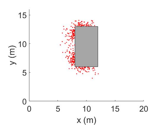
To evaluate the learning ability of Algorithm 1, N=300𝑁300N=300 samples, 𝒟={𝐱n}n=1N𝒟superscriptsubscriptsubscript𝐱𝑛𝑛1𝑁\mathcal{D}=\{\mathbf{x}_{n}\}_{n=1}^{N}, are generated according to a 2-component BRF-SNMM distribution, 𝐗(𝐱|𝚯1:NC)subscriptWeierstrass-psuperscript𝐗conditional𝐱subscript𝚯:1subscript𝑁𝐶\wp_{\mathbf{X}^{*}}(\mathbf{x}|\boldsymbol{\Theta}_{1:N_{C}}) with NC=2subscript𝑁𝐶2N_{C}=2, and deployed with the obstacle, as shown in Fig. 1 (Left). For simplicity, a binary skewing function, QY(𝐱){0,1}subscript𝑄𝑌𝐱01Q_{Y}(\mathbf{x})\in\{0,1\}, is applied to indicate if the obstacle in Fig. 1 (Left) occupies the location. The parameters of the BRF-SNMM, 𝚯1:NC={(ωi,𝚯i)}i=12subscript𝚯:1subscript𝑁𝐶superscriptsubscriptsubscript𝜔𝑖subscript𝚯𝑖𝑖12\boldsymbol{\Theta}_{1:N_{C}}=\{(\omega_{i},\boldsymbol{\Theta}_{i})\}_{i=1}^{2} are set as follows, ω1=ω2=0.5subscript𝜔1subscript𝜔20.5\omega_{1}=\omega_{2}=0.5, 𝝁1=[912]subscript𝝁1matrix912\boldsymbol{\mu}_{1}=\begin{bmatrix}9&12\end{bmatrix}, 𝚺1=[10.30.30.7]subscript𝚺1matrix10.30.30.7\boldsymbol{\Sigma}_{1}=\begin{bmatrix}1&0.3\\ 0.3&0.7\end{bmatrix}, 𝝁2=[97]subscript𝝁2matrix97\boldsymbol{\mu}_{2}=\begin{bmatrix}9&7\end{bmatrix}, and 𝚺2=[10.30.30.7]subscript𝚺2matrix10.30.30.7\boldsymbol{\Sigma}_{2}=\begin{bmatrix}1&-0.3\\ -0.3&0.7\end{bmatrix}.

In this experiment, only the sample data set, 𝒟𝒟\mathcal{D}, is available, and the parameters, NCsubscript𝑁𝐶N_{C}, and 𝚯1:NC={(ωi,𝚯i)}i=1NCsubscript𝚯:1subscript𝑁𝐶superscriptsubscriptsubscript𝜔𝑖subscript𝚯𝑖𝑖1subscript𝑁𝐶\boldsymbol{\Theta}_{1:N_{C}}=\{(\omega_{i},\boldsymbol{\Theta}_{i})\}_{i=1}^{N_{C}}, all need to be estimated. We try five component numbers, such that NC=1,2,3,4,5subscript𝑁𝐶12345N_{C}=1,2,3,4,5, to run Algorithm 1.

The learning performance of Algorithm 1 is compared with the other two approaches. 1) GMM approach: Assume that the samples are generated by an underlying GMM and the GMM’s parameters are estimated from 𝒟𝒟\mathcal{D}, 2) SNMM-GMM approach: Assume that the samples are generated by an underlying BRF-SNMM and the parameters 𝚯1:NCsubscript𝚯:1subscript𝑁𝐶\boldsymbol{\Theta}_{1:N_{C}} are estimated using the GMM parameter learning algorithm. For a fair comparison, in Algorithm 1, the SNMM is also initialized by the GMM’s parameter learning algorithm, specially, the iterative Expectation-Maximization (EM) algorithm [20].

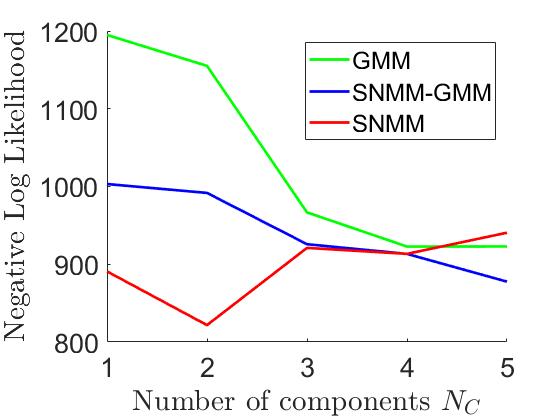
The NLLs of the samples generated based on different approaches are plotted in Fig. 1 (Right). It can be seen that only our algorithm can provide the smallest NLL at NC=2subscript𝑁𝐶2N_{C}=2. It means that the statistical model learned by our proposed Algorithm 1 can describe the samples using only two components, as equal to the component number of the ground-truth SNMM distribution. In contrast, the SNMM-GMM and GMM approaches request four or more components to describe the samples.
Refer to caption
Refer to caption
Figure 1: Left: Samples (N=300𝑁300N=300) generated according to the underlying 2-component BRF-SNMM distribution are deployed with the obstacle in the workspace. The red points indicate the samples, and the gray rectangle indicates the obstacle. Right: Comparison of parameter learning performances. The NLLs are generated by different approaches for different values of NCsubscript𝑁𝐶N_{C}.

IV-B Path-Planning for VLSR System

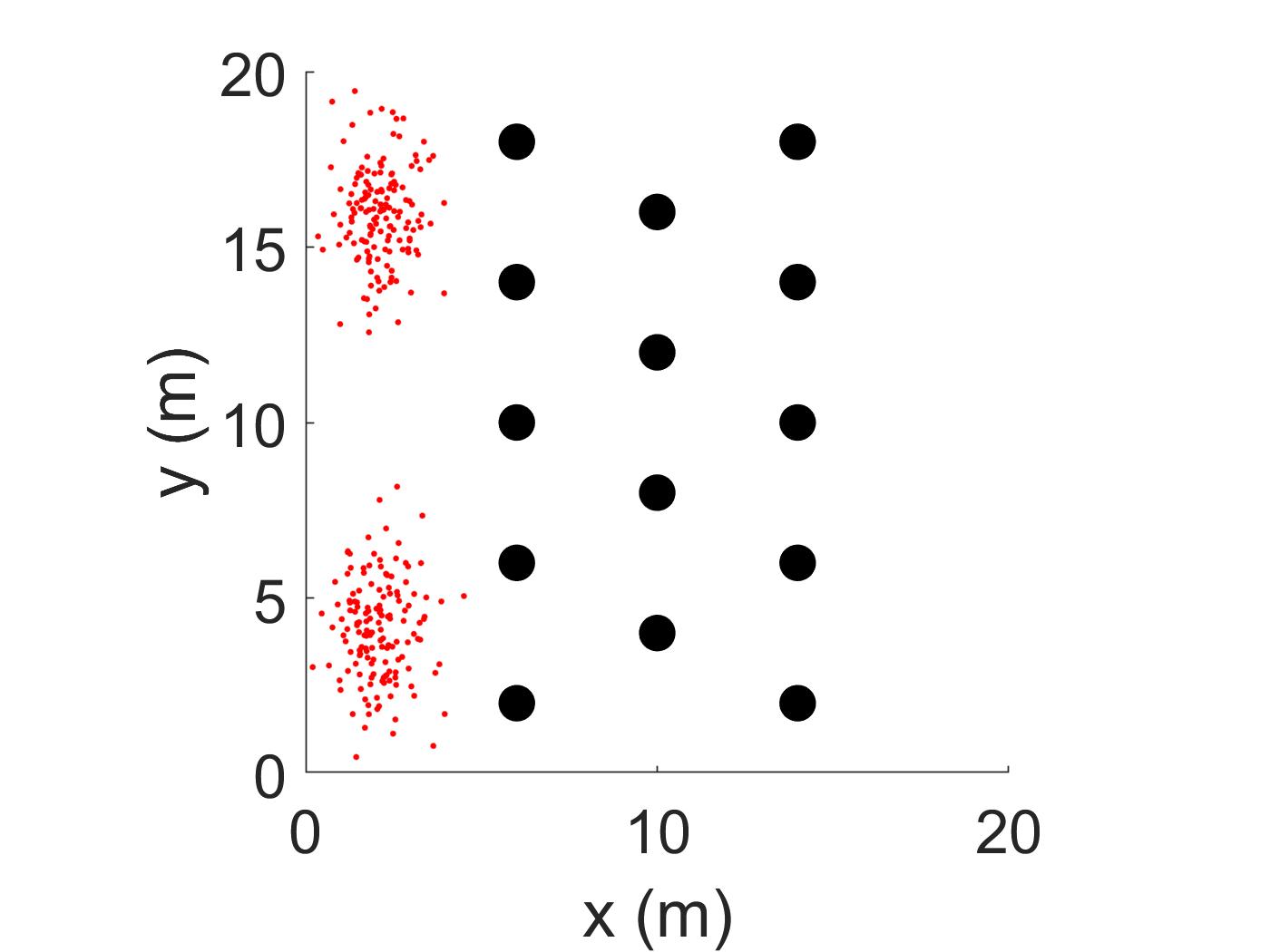
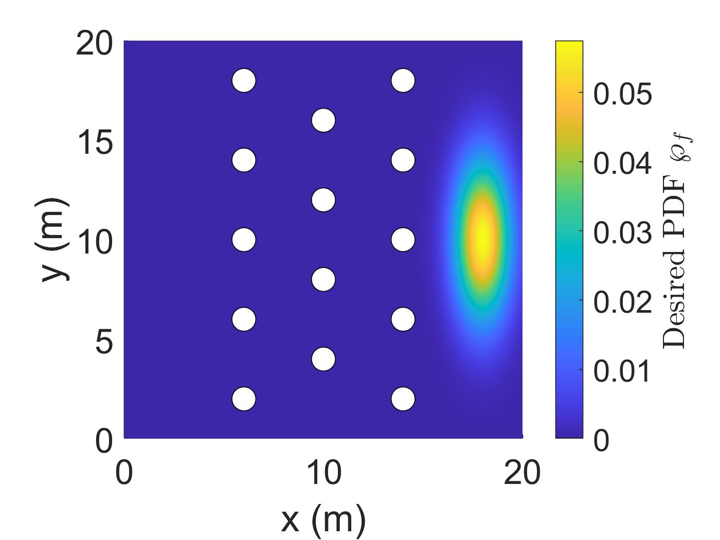
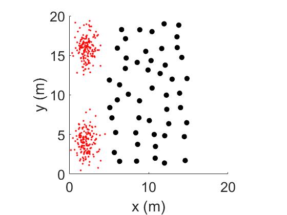
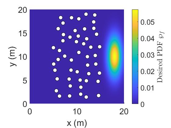
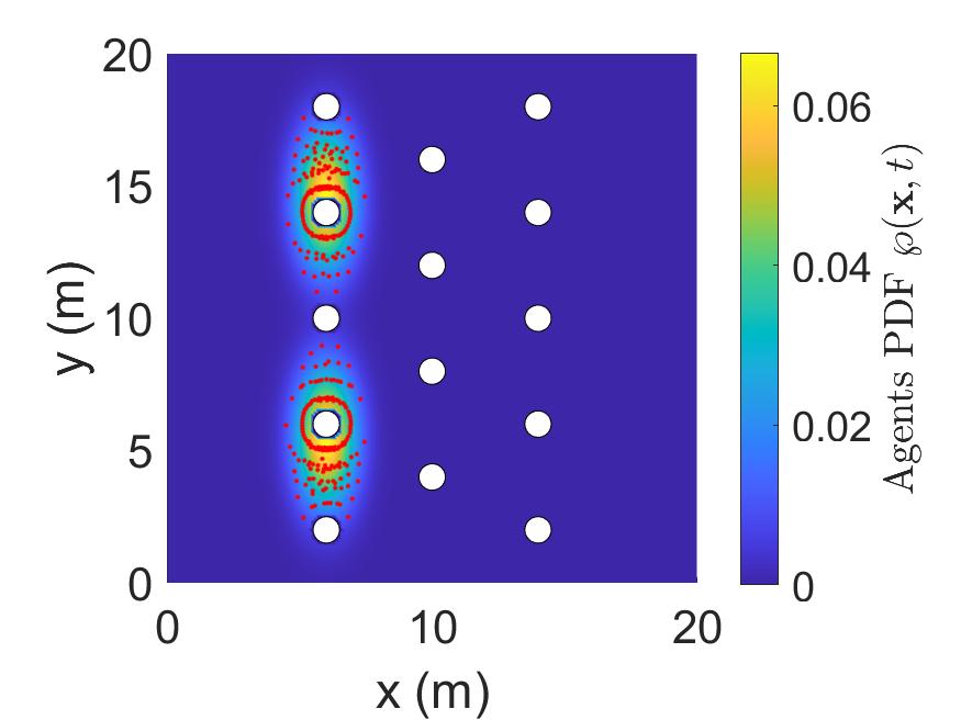
To evaluate the proposed path-planning algorithms, first, we create a simple artificial forest environment (Forest-I) shown in Fig. 2 (left), where 14 black circles indicate the trees in the artificial forest. A similar artificial forest environment has been recently applied and reported in [9]. However, unlike [9] where only 16 drones are simulated, a VLSR system comprised of N=300𝑁300N=300 agents is tested in this experiment. Given the agents’ initial positions in the artificial forest, the red points indicated by the red points in Fig. 2 (left), the goal of the path-planning task is to guide all of the agents to traverse the artificial forest and avoid collisions with these ”trees” and achieve the desired distribution, fsubscriptWeierstrass-p𝑓\wp_{f}, shown in Fig. 2 (right). The white circles shown in Fig. 2 (right) indicate the areas where QY(𝐱)=0subscript𝑄𝑌𝐱0Q_{Y}(\mathbf{x})=0, which means that agents are not allowed to go through these areas because they are occupied by ”trees.”

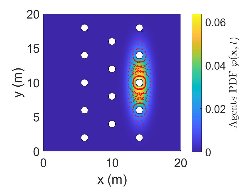
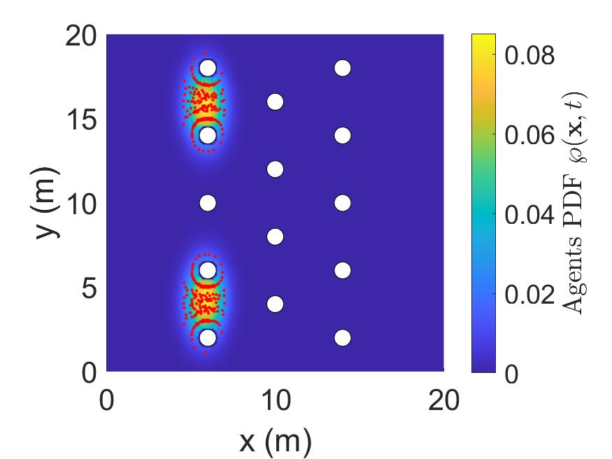
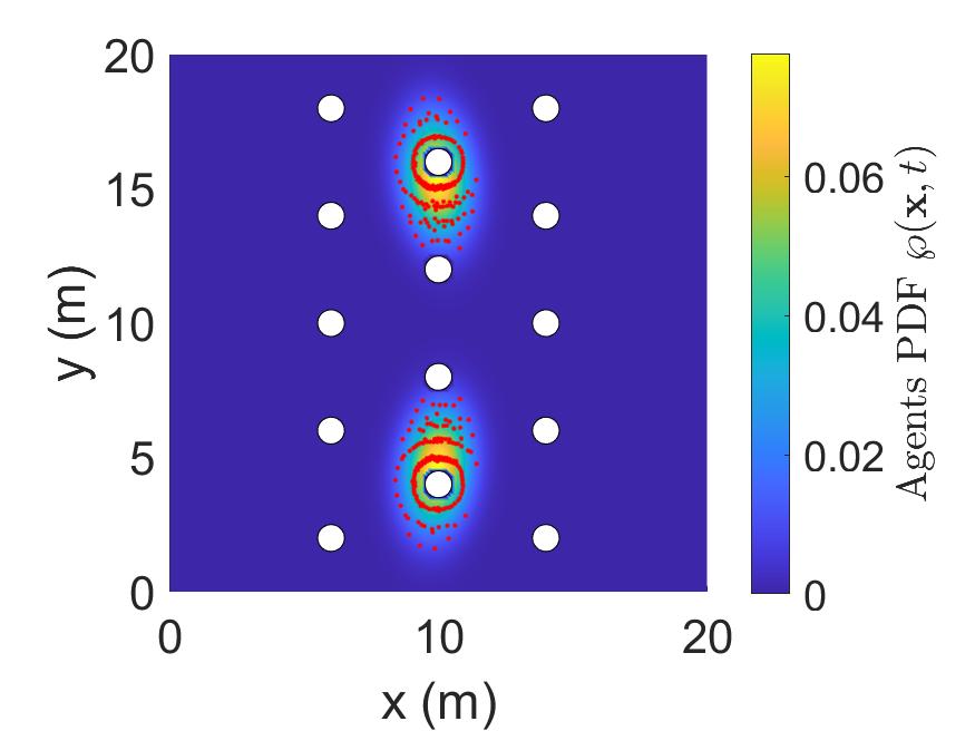
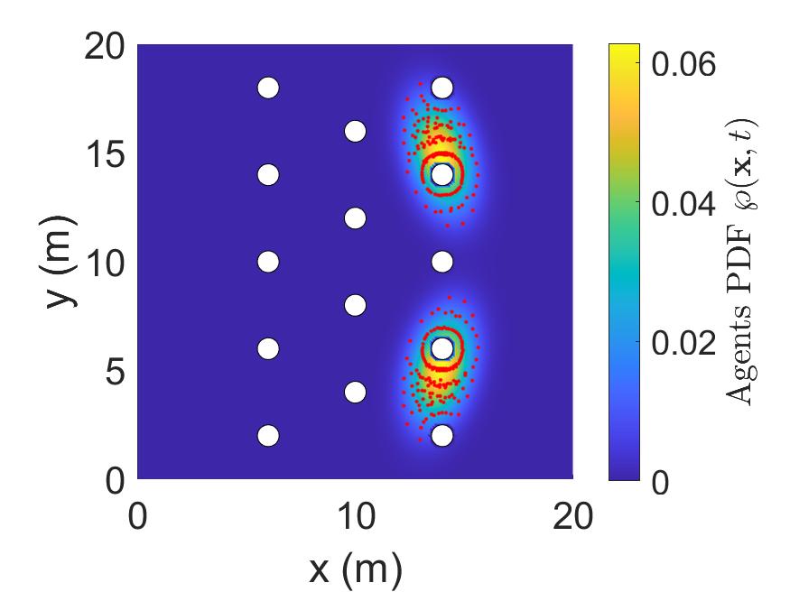
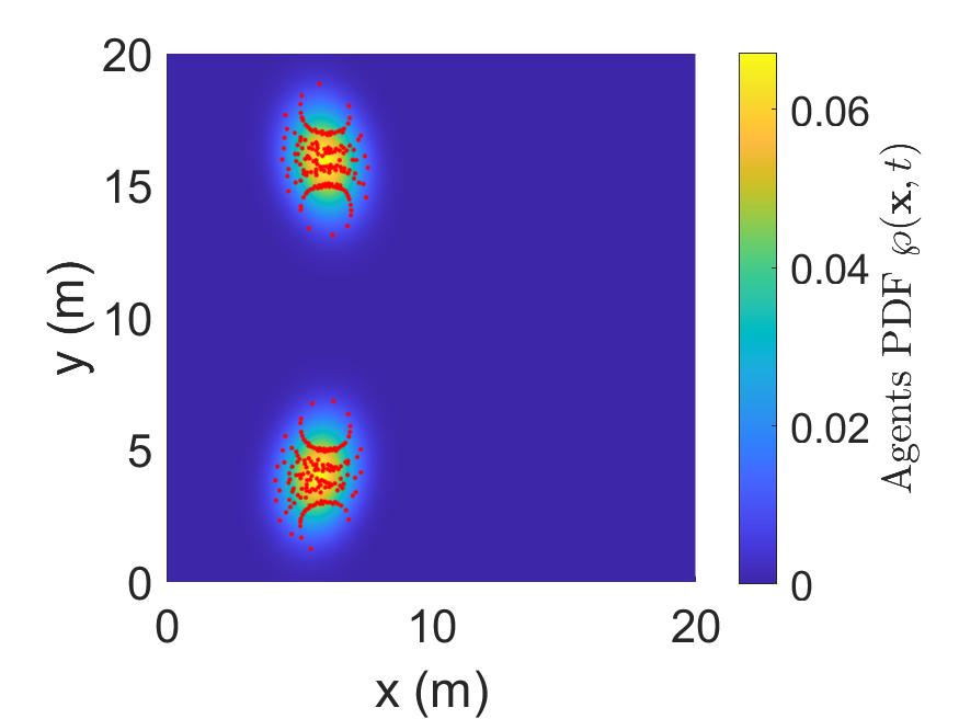
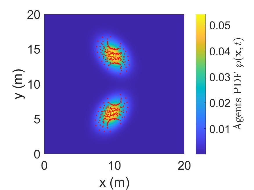
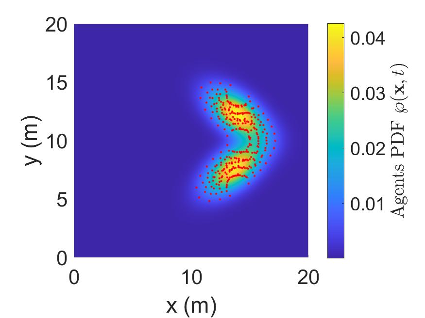
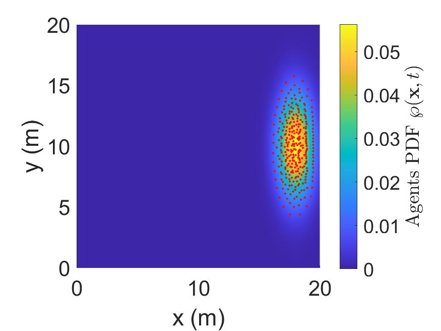
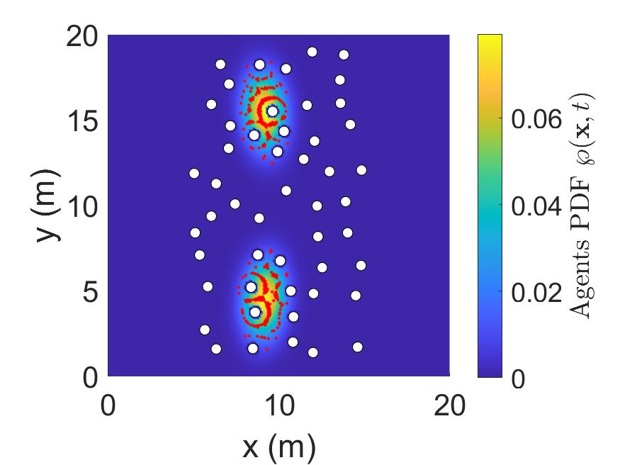
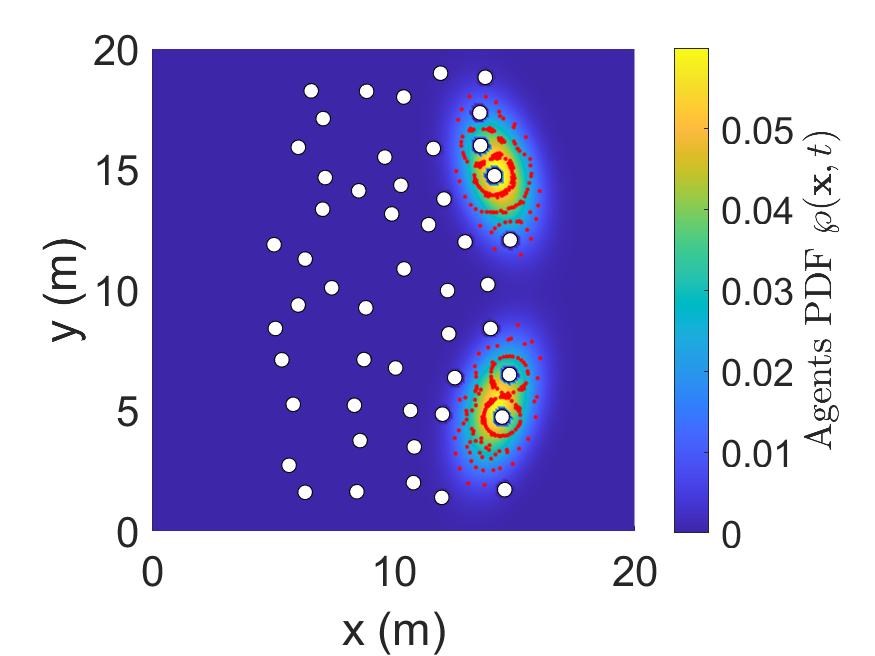
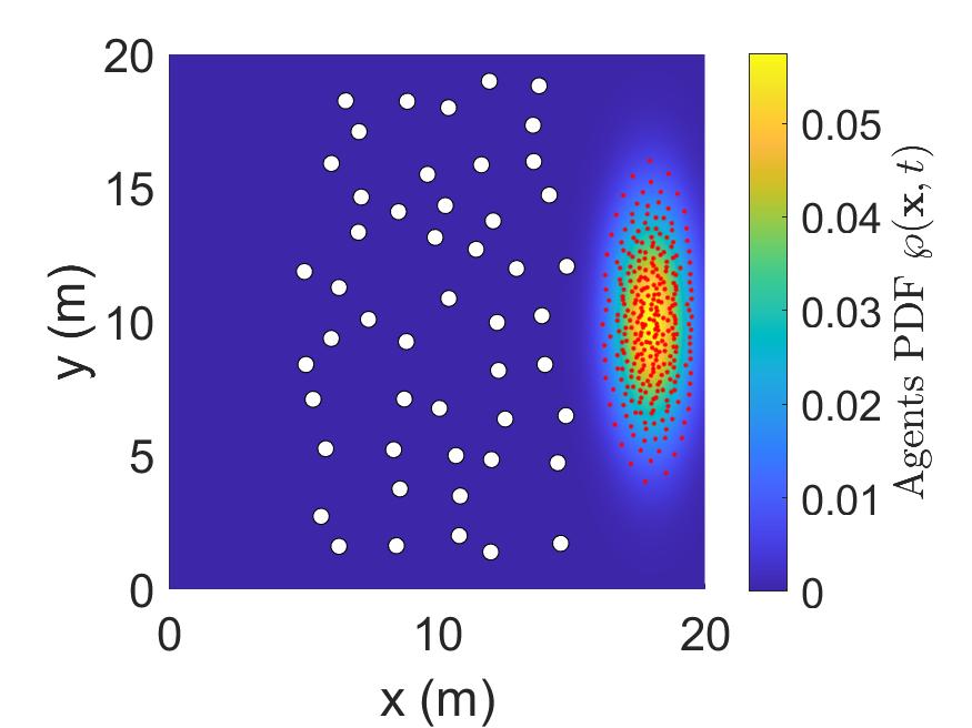
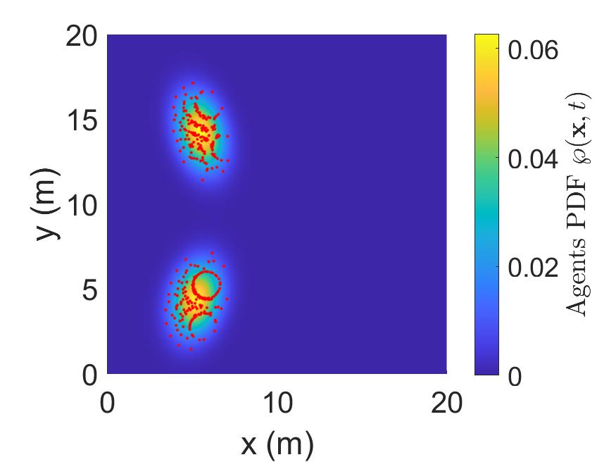
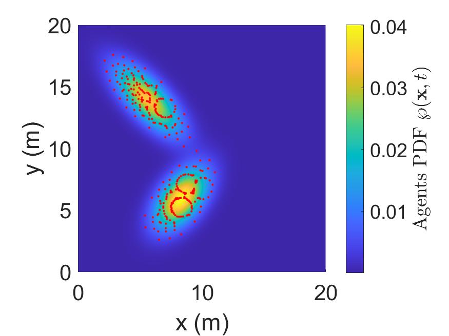
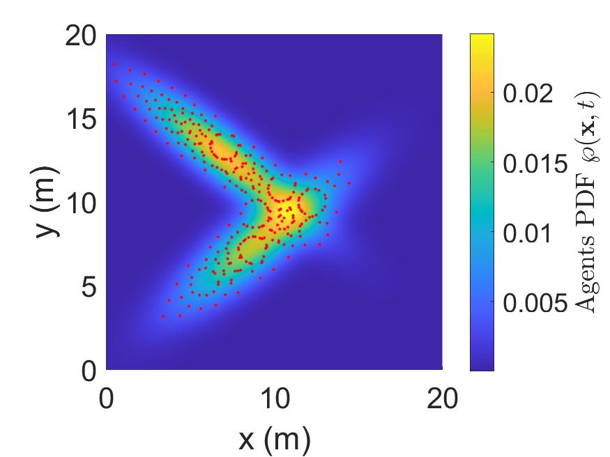
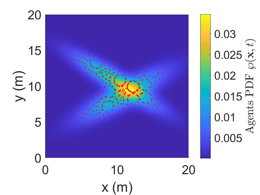
The SNMM-DI and the SNMM-APF path-planning algorithms are first executed to generate the trajectories of agents’ PDFs, where NCsubscript𝑁𝐶N_{C} is set to 2, where the SNMMs are also initialized by the GMM’s parameter learning algorithm [20] like Section IV-A. Then, the microscopic controls for individual agents are obtained to manipulate agents to traverse the artificial forest. The snapshots of trajectories of agents and corresponding PDFs generated by SNMM-DI and SNMM-APF path-planing algorithms are presented in Fig. 3 and 4, respectively. These snapshots show that both path-planning algorithms can provide acceptable performances, although different trajectories of agents’ PDFs are generated. It can also be observed that the time-varying agents’ distributions are “split” by the obstacles due to the skewing function QYsubscript𝑄𝑌Q_{Y}, which is the expected advantage of the SNMM over the GMM.

To demonstrate the explicit advantage of SNMM over GMM in path-planning problems, a GMM-based approach is also applied to the same problem for comparison. Given that the GMM can be viewed as a special case of the SNMM where QY(𝐗)1subscript𝑄𝑌𝐗1Q_{Y}(\mathbf{X})\equiv 1 according to (3), the APF-based path-planning approach can also be applied to obtain the GMM trajectory by setting QY(𝐱)=1subscript𝑄𝑌𝐱1Q_{Y}(\mathbf{x})=1 for all 𝐱𝒲𝐱𝒲\mathbf{x}\in\mathcal{W}. However, since the obstacle information is not embedded in the GMM distributions, φ(𝐱,t)𝜑𝐱𝑡\varphi(\mathbf{x},t), a repulsive potential against the skewing function is added to the potential defined in (27), such that

URep(t)𝒲φ(𝐱,t)[1Q(𝐱)]𝑑𝐱subscript𝑈𝑅𝑒𝑝𝑡subscript𝒲𝜑𝐱𝑡delimited-[]1𝑄𝐱differential-d𝐱U_{Rep}(t)\triangleq\int_{\mathcal{W}}\varphi(\mathbf{x},t)[1-Q(\mathbf{x})]d\mathbf{x} (31)

It is noteworthy that the repulsive potential becomes zero when QY(𝐱)=1subscript𝑄𝑌𝐱1Q_{Y}(\mathbf{x})=1 for all 𝐱𝒲𝐱𝒲\mathbf{x}\in\mathcal{W}, signifying a scenario with no obstacles. The range of the repulsive potential is URep[0,1]subscript𝑈𝑅𝑒𝑝01U_{Rep}\in[0,1]. The potential for the GMM-based approach can be expressed by

UGMM(t)subscript𝑈𝐺𝑀𝑀𝑡absent\displaystyle U_{GMM}(t)\triangleq γSNUSN(t|Q(𝐱)1)+γCSUCS(t|Q(𝐱)1)subscript𝛾𝑆𝑁subscript𝑈𝑆𝑁conditional𝑡𝑄𝐱1subscript𝛾𝐶𝑆subscript𝑈𝐶𝑆conditional𝑡𝑄𝐱1\displaystyle\gamma_{SN}U_{SN}(t|Q(\mathbf{x})\equiv 1)+\gamma_{CS}U_{CS}(t|Q(\mathbf{x})\equiv 1)
+\displaystyle+ γRep𝟏(URep(t),η)ln[URep(t)]subscript𝛾𝑅𝑒𝑝1subscript𝑈𝑅𝑒𝑝𝑡𝜂subscript𝑈𝑅𝑒𝑝𝑡\displaystyle\gamma_{Rep}\boldsymbol{1}(U_{Rep}(t),\eta)\ln[U_{Rep}(t)] (32)

where γRep+subscript𝛾𝑅𝑒𝑝superscript\gamma_{Rep}\in\mathbb{R}^{+} is a user-defined weight, and η[0,1]𝜂01\eta\in[0,1] is a tolerance threshold, which indicates the tolerant maximum cumulated probability of agents over the occupied areas. Finally, similarly to the SNMM-APF approach, the trajectory of agents’ PDFs is obtained by minimizing the potential, UGMM(t)subscript𝑈𝐺𝑀𝑀𝑡U_{GMM}(t), w.r.t. the parameters similarly to (16) - (18). For distinction, this GMM-based approach is referred to as the GMM-APF approach.

For a fair comparison, the same user-defined parameters as the SNMM-APF approaches are applied to the GMM-APF approach. The parameters γRepsubscript𝛾𝑅𝑒𝑝\gamma_{Rep} and η𝜂\eta are set to 111 and 5%percent55\%, respectively, and the max optimization step is set to 300030003000. In addition, the same microscopic control is also applied to generate the control inputs. The snapshots of trajectories of agents and corresponding PDFs generated by the GMM-APF algorithm are presented in Fig. 5.

The numerical comparison results are tabulated in Table I, denoted by “Forest-I”. All of the simulations are conducted by MATLAB on the same computer. The column “Time” indicates the computational time for obtaining the optimal agents’ PDFs. The column “Length” indicates the statistical results of the length of N=300𝑁300N=300 agents’ trajectories in the form of “mean ±plus-or-minus\pm standard deviation”. It can be seen that the proposed two SNMM-based approaches can outperform the GMM-based approach in terms of computational time and trajectory length. In addition, because the SNMM-DI approach does not need to solve the optimization problem, it can obtain the agents’ PDFs in a short period. However, it is also noteworthy that the absence of optimization in the SNMM-DI approach will result in a non-continuous PDF trajectory when the VLSR system travels a huge obstacle.

TABLE I: Performance Comparison
Simulation Approach Step Time Length Success?
(min) (m)
Forest-I SNMM-DI 859 1.55 19.75 ±plus-or-minus\pm 0.92 Yes
SNMM-APF 1211 54.69 27.17 ±plus-or-minus\pm 1.74 Yes
GMM-APF 2667 64.25 33.46 ±plus-or-minus\pm 2.58 Yes
Forest-II SNMM-DI 859 1.55 22.68 ±plus-or-minus\pm 1.25 Yes
SNMM-APF 1611 57.18 30.15 ±plus-or-minus\pm 1.56 Yes
GMM-APF 3000 22.35 18.07 ±plus-or-minus\pm 3.34 No
Refer to caption
Refer to caption
Figure 2: The path-planning problem for VLSR systems in the simple artificial forest environment (Forest-I simulation). Left: The red points indicate the initially deployed agents, and the black circles represent the “trees” in the forest. Right: The desired agents’ PDF is shown, where the white areas are occupied by “trees”.

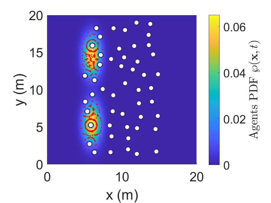
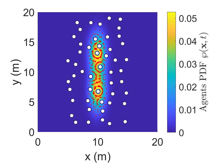
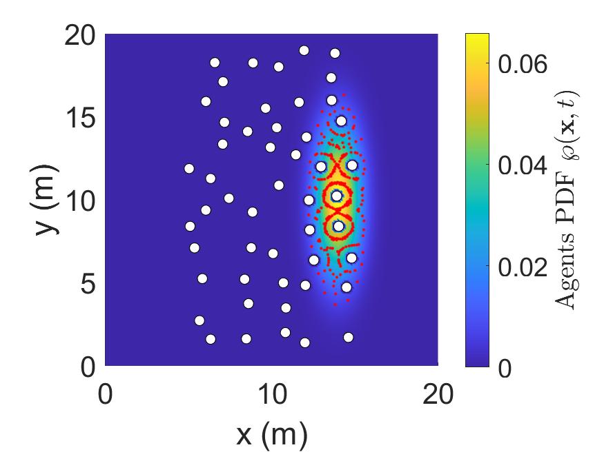
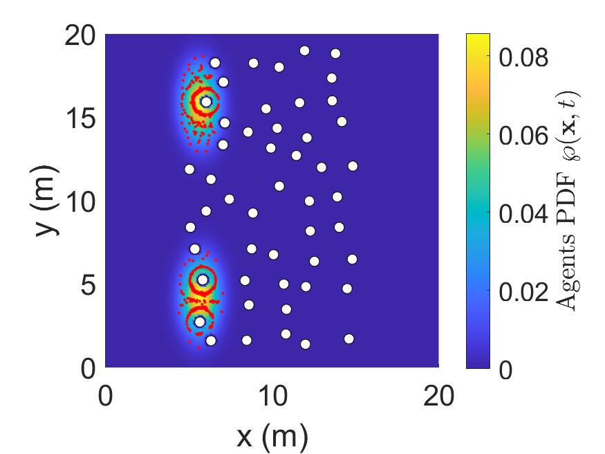
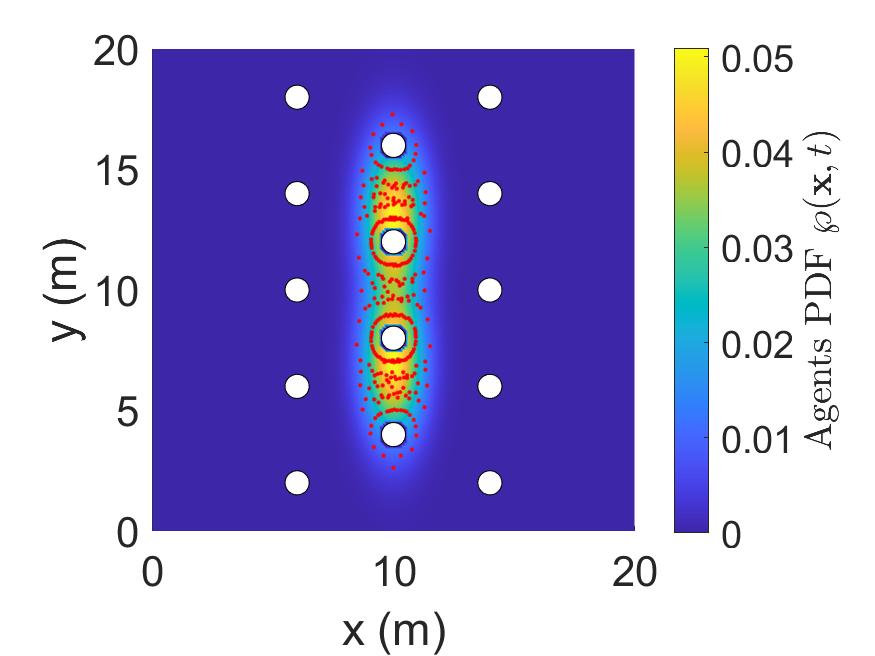
Furthermore, to demonstrate the effectiveness of the proposed SNMM-based approaches for cluttered environments, a complex artificial forest environment (Forest-II) is also considered, where 50 smaller circles are deployed randomly in the workspace to represent the trees in the forest. Then, assuming the same agents’ initial and the desired distributions, we re-conduct the simulation with the same number of components, NC=2subscript𝑁𝐶2N_{C}=2. It is found that our proposed SNMM-based approaches still work well, but the GMM-based approach fails because the potential optimization defined in (32) is stuck in the local minimum. The agents’ trajectories generated by the two SNMM-based and the GMM-based approaches are plotted in Fig. 7, 8, and 9, respectively. In addition, the corresponding numerical results are also tabulated in Table I, denoted by “Forest-II”.
Refer to caption
Refer to caption
Refer to caption
Refer to caption
Figure 3: Snapshots of the trajectory of agents and corresponding PDFs generated by the SNMM-DI approach in the Forest-I simulation.
Refer to caption
Refer to caption
Refer to caption
Refer to caption
Figure 4: Snapshots of the trajectory of agents and corresponding PDFs generated by the SNMM-APF approach in the Forest-I simulation.
Refer to caption
Refer to caption
Refer to caption
Refer to caption
Figure 5: Snapshots of the trajectory of agents and corresponding PDFs generated by the GMM-APF approach in the Forest-I simulation.
Refer to caption
Refer to caption
Figure 6: The path-planning problem for VLSR systems in the complex artificial forest environment (Forest-II simulation). Left: The red points indicate the initially deployed agents, and the black circles represent the “trees” in the forest. Right: The desired agents’ PDF is shown, where the white areas are occupied by “trees”.
Refer to caption
Refer to caption
Refer to caption
Refer to caption
Figure 7: Snapshots of the trajectory of agents and corresponding PDFs generated by the SNMM-DI approach in the Forest-II simulation.
Refer to caption
Refer to caption
Refer to caption
Refer to caption
Figure 8: Snapshots of the trajectory of agents and corresponding PDFs generated by the SNMM-APF approach in the Forest-II simulation.
Refer to caption
Refer to caption
Refer to caption
Refer to caption
Figure 9: Snapshots of the trajectory of agents and corresponding PDFs generated by the GMM-APF approach in the Forest-II simulation.

V CONCLUSIONS AND FUTURE WORK

This paper proposes a novel Bernoulli-random-field-based multivariate skew-normal distribution and the skew-normal mixture model to represent the macroscopic states of the VLSR systems. In addition, a parameter learning algorithm is provided to estimate the model parameters for the BRF-SNMM. Furthermore, two path-planning algorithms are also developed based on the SNMM to guide the VLSR systems to traverse cluttered environments. The simulations in the artificial forest environments demonstrate the effectiveness of these two path-planning algorithms and the superiority of the SNMM-based approaches over the GMM-based approach, especially in cluttered environments.

References

  • [1] M. Steinberg, J. Stack, and T. Paluszkiewicz, “Long duration autonomy for maritime systems: Challenges and opportunities,” Autonomous Robots, vol. 40, no. 7, pp. 1119–1122, 2016.
  • [2] M. Hüttenrauch, S. Adrian, G. Neumann et al., “Deep reinforcement learning for swarm systems,” Journal of Machine Learning Research, vol. 20, no. 54, pp. 1–31, 2019.
  • [3] P. Hernandez-Leal, B. Kartal, and M. E. Taylor, “A survey and critique of multiagent deep reinforcement learning,” Autonomous Agents and Multi-Agent Systems, vol. 33, no. 6, pp. 750–797, 2019.
  • [4] L. E. Parker, “Path planning and motion coordination in multiple mobile robot teams,” Encyclopedia of complexity and system science, pp. 5783–5800, 2009.
  • [5] G. Foderaro, S. Ferrari, and T. A. Wettergren, “Distributed optimal control for multi-agent trajectory optimization,” Automatica, vol. 50, no. 1, pp. 149–154, 2014.
  • [6] S. Ferrari, G. Foderaro, P. Zhu, and T. A. Wettergren, “Distributed optimal control of multiscale dynamical systems: a tutorial,” IEEE Control Systems Magazine, vol. 36, no. 2, pp. 102–116, 2016.
  • [7] K. Rudd, G. Foderaro, P. Zhu, and S. Ferrari, “A generalized reduced gradient method for the optimal control of very-large-scale robotic systems,” IEEE transactions on robotics, vol. 33, no. 5, pp. 1226–1232, 2017.
  • [8] P. Zhu, C. Liu, and S. Ferrari, “Adaptive online distributed optimal control of very-large-scale robotic systems,” IEEE Transactions on Control of Network Systems, vol. 8, no. 2, pp. 678–689, 2021.
  • [9] E. Soria, F. Schiano, and D. Floreano, “Distributed predictive drone swarms in cluttered environments,” IEEE Robotics and Automation Letters, vol. 7, no. 1, pp. 73–80, 2021.
  • [10] A. Azzalini, “A class of distributions which includes the normal ones,” Scandinavian journal of statistics, pp. 171–178, 1985.
  • [11] A. Azzalini and A. D. Valle, “The multivariate skew-normal distribution,” Biometrika, vol. 83, no. 4, pp. 715–726, 1996.
  • [12] A. K. Gupta, G. Gonzalez-Farias, and J. A. Dominguez-Molina, “A multivariate skew normal distribution,” Journal of multivariate analysis, vol. 89, no. 1, pp. 181–190, 2004.
  • [13] R. B. Arellano-Valle and M. G. Genton, “On fundamental skew distributions,” Journal of Multivariate Analysis, vol. 96, no. 1, pp. 93–116, 2005.
  • [14] F. Ramos and L. Ott, “Hilbert maps: Scalable continuous occupancy mapping with stochastic gradient descent,” The International Journal of Robotics Research, vol. 35, no. 14, pp. 1717–1730, 2016.
  • [15] J. Morelli, P. Zhu, B. Doerr, R. Linares, and S. Ferrari, “Integrated mapping and path planning for very large-scale robotic (vlsr) systems,” in 2019 International Conference on Robotics and Automation (ICRA).   IEEE, 2019, pp. 3356–3362.
  • [16] P. Zhu, S. Ferrari, J. Morelli, R. Linares, and B. Doerr, “Scalable gas sensing, mapping, and path planning via decentralized hilbert maps,” Sensors, vol. 19, no. 7, p. 1524, 2019.
  • [17] R. Durrett, Probability: theory and examples.   Cambridge university press, 2019, vol. 49.
  • [18] Y. Chen, T. T. Georgiou, and A. Tannenbaum, “Optimal transport for gaussian mixture models,” IEEE Access, vol. 7, pp. 6269–6278, 2018.
  • [19] K. Kampa, E. Hasanbelliu, and J. C. Principe, “Closed-form cauchy-schwarz pdf divergence for mixture of gaussians,” in The 2011 International Joint Conference on Neural Networks.   IEEE, 2011, pp. 2578–2585.
  • [20] D. Peel and G. MacLahlan, “Finite mixture models,” John & Sons, 2000.