Properties and maximum likelihood estimation of the gamma–normal and related probability distributions

Abstract

This paper presents likelihood–based inference methods for the family of univariate gamma–normal distributions $\mathrm{GN}(\alpha,r,\mu,\sigma^{2})$ that result from summing independent $\gamma(\alpha,r)$ and $N(\mu,\sigma^{2})$ random variables. First, the probability density function of a gamma–normal variable is provided in compact form with the use of parabolic cylinder functions, along with key properties. We then provide analytic expressions for the maximum–likelihood score equations and the Fisher information matrix, and discuss inferential methods for the gamma–normal distribution. Given the widespread use of the two constituting distributions, the gamma–normal distribution is a general purpose tool for a variety of applications. In particular, we discuss two distributions that are obtained as special cases and that are featured in a variety of statistical applications: the exponential–normal distribution and the chi–squared–normal (or overdispersed chi–squared) distribution.

[1]organization=Department of Physics and Astronomy, University of Alabama in Huntsville, postcode=35899, city=Huntsville, AL, country=USA [2]organization=Department of Statistics and Actuarial Science, University of Iowa, city=Iowa City, IA, postcode=52242

1 Introduction

The sum of two random variables occurs frequently in statistical applications. For example, it is often required to modify certain distributions with the addition of an independent normal distribution, as a simple means to shift the mean and/or increase the variance of the original distribution, or to model a given signal as the sum of two independent components, such as the source and the background.

For this class of applications, the exponential–normal (or exponential–Gaussian) distribution, which is the distribution of $Z=X+Y$ when $X$ is an exponential random variable and $Y$ an independent normal random variable, has been used in a variety of disciplines including chromatography (Delley, 1985; Gruskha, 1972), cellular biology (e.g. Golubev, 2010), finance (e.g. Carr et al., 2009) and psychology (e.g. Palmer et al., 2011). The gamma–normal distribution was also proposed as a generalization of the exponential–normal distribution by Plancade et al. (2012), for the specific task of proper background subtraction in certain biological applications (e.g. Xie et al., 2009; Wang and Ye, 2012). Moreover, the distribution of the sum of independent normal and chi–squared variables also occurs as the parent distribution for the goodness–of–fit statistic in Poisson regression with systematic errors, as was previously shown by one of the authors (i.e., the overdispersed chi–squared distribution, Bonamente, 2023).

While the convolution of virtually any two distributions can be carried out numerically, there are advantages to having an analytic form for the probability density function (pdf) of the sum of two random variables. One of these is computational speed and precision. In fact, the computational cost of the convolution of two distributions is typically $O(n^{2})$, where $n$ is the number of samples in the convolution (e.g. Karas and Svoboda, 2013), and this may become prohibitively high in certain applications that require high precision. Second, an explicit compact form for the density makes it easier to identify the role played by the parameters, thus making the distribution easier to use, interpret, and estimate.

Accordingly, the goal of this paper is two–fold. First, it presents a compact form for the pdf and properties of the family of gamma–normal $\mathrm{GN}(\alpha,r,\mu,\sigma^{2})$ random variables that result from the sum of a gamma $\gamma(\alpha,r)$ random variable and an independent normal $N(\mu,\sigma^{2})$ random variable.  Although the problem is elementary in its methods, a compact form for the convolution of these two distributions has not previously reported in the literature (see, e.g., the comment after Eq. 6 of Plancade et al., 2012). Given the wide use of the two constituting distributions, the univariate normal–gamma distribution is therefore a convenient general–purpose statistical tool. Secondly, the paper provides maximum likelihood score functions and the information matrix in analytic forms that are suitable for parameter estimation, and discusses possible applications for this family of distributions, including the special cases of the exponential–normal $\mathrm{EN}(\alpha,\mu,\sigma^{2})$ and the overdispersed $\chi^{2}$ distribution $\mathrm{B}(r,\mu,\sigma^{2})$.

This paper is structured as follows. Section 2 presents the probability distribution function and key properties of the gamma–normal distribution. Section 3 discusses two special cases, viz. the exponential–normal and the overdispersed chi–squared distributions. Section 4 then describes likelihood-based methods for the estimation of the gamma–normal and associated distributions. A brief review of applications of these distributions is then provided in Section 5, followed by our conclusions in Section 6.

2 The univariate gamma–normal random variable

We start by defining the normal–gamma variable as the sum of independent gamma and normal random variables (one of each). A similar name (normal–gamma or gamma–normal) is often used to describe a bivariate distribution with pdf given by the product of the gamma and normal pdfs, which is of common use in Bayesian statistics (e.g., Bernardo and Smith, 2000, p. 136). To distinguish between the two different distributions, the family of distributions under investigation in this paper is referred to as the univariate gamma–normal distribution. The qualifier will often be omitted for the sake of brevity, since all distributions discussed in this paper are univariate.

2.1 Definition

Let $X\sim\gamma(\alpha,r)$ and $Y\sim N(\mu,\sigma^{2})$ be two independent random variables, having respectively a gamma distribution with rate parameter $\alpha$ and shape parameter $r$, and a normal distribution with mean $\mu$ and variance $\sigma^{2}$. Let $Z=X+Y$ be the sum of the two variables. The pdf of $Z$ is given by the convolution of the two densities,

$$f_{Z}(z;\alpha,r,\mu,\sigma^{2})= f_{\gamma}(z;\alpha,r)*f_{N}(z;\mu,\sigma^{2})$$ (1)

$$= \int_{-\infty}^{\infty}f_{\gamma}(z-y;\alpha,r)f_{N}(y;\mu,\sigma^{2})\,dy,\;\text{ for $z-y>0$}.$$

With the substitution $x=z-y>0$, the pdf of $Z$ becomes

$$f_{Z}(z;\alpha,r,\mu,\sigma^{2})=\dfrac{\alpha^{r}}{\Gamma(r)}\dfrac{1}{\sqrt{2\pi\sigma^{2}}}\int_{0}^{\infty}x^{r-1}e^{-\alpha x}e^{-{(x-(z-\mu))^{2}}/{2\sigma^{2}}}\,dx,\;\text{ for $z\in\mathbb{R}$.}$$ (2)

The variable $Z$ with pdf given by (2) is said to belong to the family of univariate gamma–normal random variables, and it will be indicated as

$$Z\sim\mathrm{GN}(\alpha,r,\mu,\sigma^{2}).$$ (3)

$Z$ is a real–valued variable, $z\in\mathbb{R}$, with parameters $\alpha,r\in\mathbb{R}^{+}$, $\mu\in\mathbb{R}$, and $\sigma^{2}\in\mathbb{R}^{+}$.

2.2 The probability density function

The pdf of a $Z\sim\mathrm{GN}(\alpha,r,\mu,\sigma^{2})$ gamma–normal variable can be written as a function of parabolic cylinder functions $D_{p}(z)$, which are solutions of the Weber differential equation (Weber, 1869) that results from separating the variables of the wave equation in parabolic cylindrical coordinates (see also Whittaker, 1902). The parabolic cylinder functions can be written in integral form as

$$D_{p}(z)=\dfrac{e^{-z^{2}/4}}{\Gamma(-p)}\int_{0}^{\infty}e^{-xz-x^{2}/2}x^{-1-p}dx,\text{ for real $p<0$}.$$ (4)

In general $z$ may be a complex number in the argument of the parabolic cylinder function, but for this application it is only interesting to consider real values of the variable. An alternative notation for the parabolic cylinder functions is $U(a,z)=D_{-a-\nicefrac{{1}}{{2}}}(z)$ (e.g. Miller, 1952).

The pdf of a $\mathrm{GN}(\alpha,r,\mu,\sigma^{2})$ random variable can therefore be written in compact form as

$$f_{\mathrm{GN}}(z;\alpha,r,\mu,\sigma^{2})=\dfrac{(\alpha\sigma)^{r}}{\sqrt{2\pi\sigma^{2}}}\;D_{-r}\left(\zeta\right)\cdot E(z),$$ (5)

where

$$\zeta=\alpha\sigma+\dfrac{(\mu-z)}{\sigma}$$ (6)

is the argument of the parabolic cylinder function, and $E(z)$ is an exponential function with

$$\ln E(z)=-\dfrac{1}{4}\left(\sigma\alpha+\tfrac{(z-\mu)}{\sigma}\right)^{2}+\dfrac{\sigma^{2}\alpha^{2}}{2}=\dfrac{\zeta^{2}}{4}-\dfrac{(z-\mu)^{2}}{2\sigma^{2}}.$$ (7)

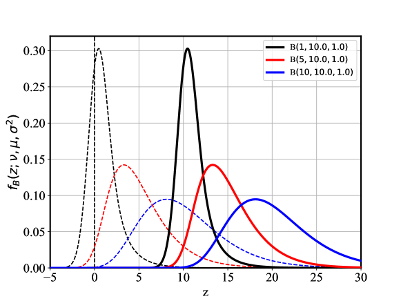
Equation 5 is the most compact form for the pdf of the gamma–normal distribution, which can be evaluated via a parabolic cylinder function and elementary functions. The general behavior of the pdf of the $\mathrm{GN}(\alpha,r,\mu,\sigma^{2})$ is illustrated in Fig. 1. Key features are a shift by $+\mu$ with respect to the $\gamma(\alpha,r)$ pdf (illustrated as a dotted curve), a broadening of the distribution, and a negative tail that is not present in the gamma distribution.

Figure 1: The gamma–normal $\mathrm{GN}(\alpha,r,\mu,\sigma^{2})$ distribution for selected values of the the rate parameter of the $\gamma$ distribution ($\alpha=1,\nicefrac{{1}}{{2}}$) and of the variance of the normal distribution ($\sigma=2,1$), and two reference values for the shape parameter of the gamma distribution ($r=5$) and the mean of the normal ($\mu=10$).

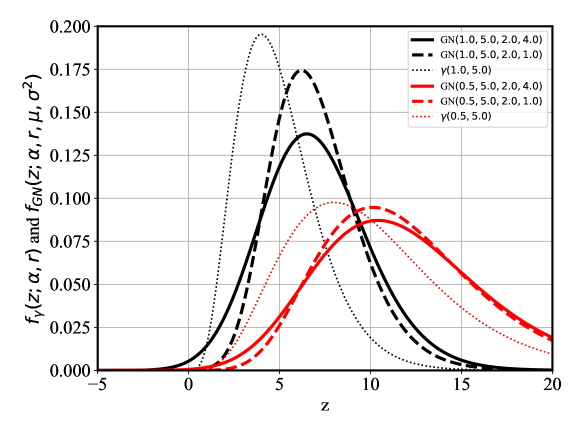
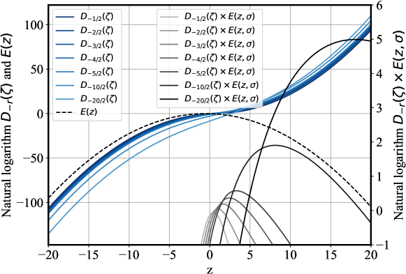
Figure 2 further illustrates the behavior of the two functions $D_{-r}(\zeta)$ and $E(z)$ and of their product, which is proportional to the pdf of the distribution according to (5). Given the large dynamical range of both functions, it is convenient to work with the logarithms of the two functions.

For comparison, we report the form of the pdf of the gamma–normal distribution as provided by Plancade et al. (2012), who first introduced it:

$$f^{\textrm{ng}}_{\mu,\sigma,k,\theta}(x)=\int f_{k,\theta}^{\textrm{gam}}f^{\textrm{norm}}_{\mu,\sigma}(x-t)dt$$ (8)

where $k$ is the shape parameter and $\theta$ the scale parameter of the gamma distribution. Their expression is equivalent to (1), and the integral was evaluated numerically by way of a Fast Fourier Transform.

2.3 Key properties

Property 1 (Translation property with respect to the $\mu$ parameter).

The pdf of the gamma–normal distribution has the property

$$f_{\mathrm{GN}}(z-\mu;\alpha,r,\mu,\sigma^{2})=f_{\mathrm{GN}}(z;\alpha,r,\mu=0,\sigma^{2}).$$ (9)

This property derives from the fact that the $\mu$ parameter enters the pdf only as a function of $(z-\mu)$. This is the same translation property that the normal distribution has. The $\mu$ parameter is therefore simply a location parameter that does not otherwise affect the shape of the distribution.

Figure 2: Parabolic cylinder functions $D_{-r}(\zeta)$ as a function of the argument $z$, with $\zeta$ according to (6), and for selected values of the shape parameter $r$. The mean of the normal was set to $\mu=0$, the variance to a fiducial value of $\sigma=1$, and the rate parameter was also fixed at $\alpha=\nicefrac{{1}}{{2}}$. On the right scale are values of the product of the parabolic cylinder function with the exponential function $E(z)$ according to (7), which is an unnormalized version of the pdf according to (5).

Property 2 (Mean, Variance, and Skewness).

The mean, variance, and skewness of a $Z\sim\mathrm{GN}(\alpha,r,\mu,\sigma^{2})$ variable are

$$\begin{cases}\text{E}[Z]=\mu+\dfrac{r}{\alpha}\\[10.0pt] \text{Var}(Z)=\sigma^{2}+\dfrac{r}{\alpha^{2}}\\ \text{E}\{[Z-E(Z)]^{3}\}=\dfrac{2}{\sqrt{r}}.\end{cases}$$

This property is an immediate consequence of the independence of the $X$ and $Y$ variables and the moments of the respective distributions.

Property 3 (Large–mean normal approximation).

For large values of $r/\alpha$, where $r$ is the shape parameter and $\alpha$ the rate parameter of the gamma distribution,

$$\mathrm{GN}\overset{a}{\sim}N((r/\alpha)+\mu,(r/\alpha^{2})+\sigma^{2}),$$

This asymptotic convergence in distribution of a $X\sim\gamma(\alpha,r)$ variable to a $N(r/\alpha,r/\alpha^{2})$ for large values of the mean $r/\alpha$ of the gamma distribution is a direct consequence of the central limit theorem, since a gamma distribution is the sum of $r$ independent exponential random variables with finite mean and variance (see, e.g., Hogg et al., 2023).

Property 4 (Closedness under convolution for fixed $\alpha$).

Let $Z_{1}$ and $Z_{2}$ be two independent gamma–normal random variables with the same $\alpha$ parameter, i.e., $Z_{1}\sim\mathrm{GN}(\alpha,r_{1},\mu_{1},\sigma_{1}^{2})$ and $Z_{2}\sim\mathrm{GN}(\alpha,r_{2},\mu_{2},\sigma_{2}^{2})$. Then

$$Z_{1}+Z_{2}\sim\mathrm{GN}(\alpha,r_{1}+r_{2},\mu_{1}+\mu_{2},\sigma_{1}^{2}+\sigma_{2}^{2}).$$

This property is an immediate consequence of the independence of the random variables, and the additive properties of the gamma and normal distributions. Specifically, if $X_{1}\sim\gamma(\alpha,r_{1})$ and $X_{2}\sim\gamma(\alpha,r_{2})$ are independent, then $X_{1}+X_{2}\sim\gamma(\alpha,r_{1}+r_{2})$; and if $Y_{1}\sim N(\mu_{1},\sigma_{1}^{2})$ and $Y_{2}\sim N(\mu_{2},\sigma_{2}^{2})$, then $Y_{1}+Y_{2}\sim N(\mu_{1}+\mu_{2},\sigma^{2}_{1}+\sigma_{2}^{2})$. This property extends to the sum of any number of independent variables and it also means that, for a fixed $\alpha$, the gamma–normal distribution is infinitely divisible.

3 Special cases of the gamma–normal distribution

This section describes special cases of the gamma–normal distribution and their properties, for certain choices of the four parameters, that are of common use in probability and in statistical applications.

3.1 The exponential–normal distribution

When the shape parameter of the gamma distribution is $r=1$, the gamma distribution becomes an exponential distribution with rate parameter $\alpha$ (or scale parameter $1/\alpha$). For $r=1$, the pdf of the gamma–normal distribution can be simplified making use of

$$D_{-1}(z)=e^{z^{2}/4}\sqrt{\dfrac{\pi}{2}}\left(1-\text{erf}\left(\dfrac{z}{\sqrt{2}}\right)\right)$$ (10)

where $\text{erf}(x)$ is the error function (see 9.254.1 of Gradshteyn and Ryzhik, 2007, and A).

A random variable $Z\sim\mathrm{GN}(r=1,\alpha,\mu,\sigma^{2})$ is therefore said to be an exponential–normal or exponential–Gaussian variable $Z\sim\mathrm{EN}(\alpha,\mu,\sigma^{2})$, with probability distribution function

$$f_{\mathrm{EN}}(z)=\dfrac{\alpha}{2}\left(1-\text{erf}(\zeta/\sqrt{2})\right)e^{\zeta^{2}/2}E(z),$$ (11)

where

$$\begin{cases}\zeta=\alpha\sigma+\dfrac{\mu-z}{\sigma}\\[10.0pt] \ln E(z)=\dfrac{\alpha}{2}\left(2(\mu-z)+\sigma^{2}\alpha\right).\end{cases}$$ (12)

This distribution is the same exponential–normal distribution that has been used for chromatography and other applications (see, e.g. Gruskha, 1972; Delley, 1985). The pdf in Equation 11 is equivalent to the one used by various authors in this field, including Kalambet et al. (2011); Xie et al. (2009).

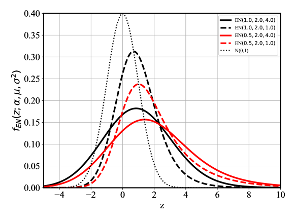
Figure 3 illustrates the behavior of the pdf of the exponential–normal distribution, which features a mean $\text{E}[Z]=\mu+1/\alpha$ and a variance $\text{Var}(Z)=\sigma^{2}+1/\alpha^{2}$. The effect of the convolution with an exponential is to increase both the mean and variance of the normal distribution. Additional properties were studied in Gruskha (1972).

Figure 3: Probability density function of an exponential–normal variable $\mathrm{EN}(\alpha,\mu,\sigma^{2})$, for a value $\mu=0$ and selected values of the $\alpha$ and $\sigma^{2}$ parameters.

3.2 The chi–squared–normal or overdispersed chi–squared distribution

When $\alpha=\nicefrac{{1}}{{2}}$ and we set $r=\nicefrac{{\nu}}{{2}}$, the gamma distribution $\gamma(\alpha,r)$ becomes a chi–squared distribution $\chi^{2}(\nu)$ with degrees of freedom parameter $\nu$. The chi–squared distribution (e.g. Helmert, 1876; Fisher, 1924) has occupied a central role in statistics since K. Pearson’s introduction of the $\chi^{2}$ test of goodness of fit (Pearson, 1900). One of its uses in statistics is as the parent distribution of a number of goodness–of–fit statistics that are in common use. One of the most common uses is for normal data, whereas chi–squared is the parent distribution of the Gaussian log–likelihood statistic obtained from maximum–likelihood optimization (often referred to as the $\chi^{2}$ or $S$ statistic, e.g. Fisher, 1925). In many statistical applications, $\nu\in\mathbb{N}$ is an integer number of degrees of freedom of the distribution, but the properties derived in this paper apply to the more general case of a positive real $\nu$ parameter.

A random variable $Z\sim\mathrm{GN}(r=\nicefrac{{\nu}}{{2}},\alpha=\nicefrac{{1}}{{2}},\mu,\sigma^{2})$ is said to be a chi–squared–normal or an overdispersed chi–squared variable $Z\sim\mathrm{B}(\nu,\mu,\sigma^{2})$. Its probability distribution function is given, according to (5), by

$$f_{B}(z;\nu,\mu,\sigma^{2})=\dfrac{1}{2^{\nu/2}\sqrt{2\pi}\;\sigma^{1-\nu/2}}D_{-\nu/2}\left(\zeta\right)\cdot E(z,\sigma),$$ (13)

where

$$\begin{cases}\zeta=\dfrac{\sigma}{2}+\dfrac{(\mu-z)}{\sigma}\\[10.0pt] \ln E(z,\sigma)=-\left(\tfrac{\sigma^{2}+2(z-\mu)}{4\sigma}\right)^{2}+\dfrac{\sigma^{2}}{8}.\end{cases}$$ (14)

The mean is $\text{E}[Z]=\mu+\nu$, and the variance is $\text{Var}(Z)=2\nu+\sigma^{2}$.

Figure 4: Probability density function of the overdispersed chi–squared variable $B(\nu,\mu=0,\sigma^{2})$ for a fiducial value of the number of degrees of freedom, and as a function of the overdispersion parameter $\sigma^{2}$.

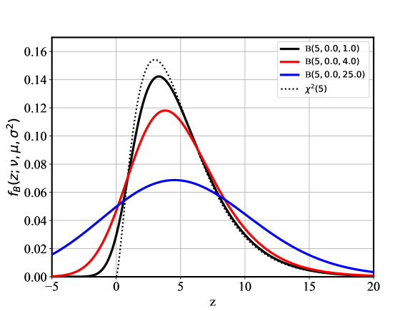
Figure 4 illustrates the pdf of a $B(\nu,\mu,\sigma^{2})$ variable for $\mu=0$ and a fixed value of $\nu$, as a function of the overdispersion parameter $\sigma^{2}$. The broadening of the distribution with increasing $\sigma^{2}$ is the reason for the name overdispersed $\chi^{2}$ distribution, and it leads to a tail of negative values that is not present in the $\chi^{2}(\nu)$ distribution. Figure 5 illustrates the behavior of the $B(\nu,\mu,\sigma^{2})$ distribution as a function of the number of degrees of freedom, for a fiducial value of the $\mu$ and $\sigma^{2}$ parameters. The corresponding $B(\nu,\mu=0,\sigma^{2})$ are also plotted as dashed curves to illustrate the translation property (Property 1). The overdispersed chi–squared distribution was first introduced by one of the authors (Bonamente, 2023) for the case of $\mu=0$, and its density is now provided in full form in (13).

Property 5 (Closedness over convolution of the overdispersed chi–squared distribution).

Let $Z_{1}\sim\mathrm{B}(\nu_{1},\mu_{1},\sigma^{2}_{1})$ and $Z_{2}\sim\mathrm{B}(\nu_{2},\mu_{2},\sigma^{2}_{2})$ be two independent overdispersed chi–squared distribution. Then

$$Z_{1}+Z_{2}\sim\mathrm{B}(\nu_{1}+\nu_{2},\mu_{1}+\mu_{2},\sigma^{2}_{1}+\sigma^{2}_{2})$$

This is an immediate consequence of Property (4), and it applies to the sum of any number of independent overdispersed chi–squared variables. This means that the overdispersed chi–squared distribution is infinitely divisible.

Figure 5: Probability density function of the overdispersed chi–squared variable $B(\nu,\mu,\sigma^{2})$ for fiducial values of the $\mu$ and $\sigma^{2}$ parameters, and for selected values of the number of degrees of freedom $\nu$. The bias parameter $\mu$ only provides a shift of the distributions by a fixed amount $+\mu$ relative to the corresponding $\mu=0$ distributions, which are plotted as dashed curves.

Table 1: Selected percentiles or one–sided upper critical values of the $B(\nu,\mu=0,\sigma^{2})$ family of distributions for $\nu=1,2,3,4,5$ and 10, and for representative values of the overdispersion parameter $\sigma^{2}$. The $\chi^{2}$ entries correspond to the case of no overdispersion.

$\sigma$	100$p$th percentile
	$p=0.5$ (median)
	Number of d.o.f. ($\nu$)
	1	2	3	4	5	10
1	0.738	1.577	2.492	3.448	4.423	9.376
2	0.859	1.752	2.671	3.612	4.568	9.462
5	0.959	1.922	2.888	3.857	4.829	9.722
10	0.988	1.976	2.964	3.953	4.942	9.894
$\chi^{2}$	0.455	1.386	2.366	3.357	4.351	9.342
	$p=0.90$
	Number of d.o.f. ($\nu$)
	1	2	3	4	5	10
1	3.067	4.855	6.460	7.964	9.404	16.111
2	4.061	5.584	7.066	8.499	9.891	16.475
5	7.659	8.907	10.149	11.386	12.617	18.688
10	13.947	5.078	16.207	17.335	18.462	24.081
$\chi^{2}$	2.706	4.605	6.251	7.779	9.236	15.987
	$p=0.95$
	Number of d.o.f. ($\nu$)
	1	2	3	4	5	10
1	4.163	6.241	8.032	9.684	11.252	18.447
2	5.171	6.988	8.673	10.262	11.785	18.861
5	9.603	10.969	12.322	13.662	14.990	21.469
10	17.632	18.813	19.991	21.168	22.343	28.190
$\chi^{2}$	3.841	5.991	7.815	9.488	11.070	18.307
	$p=0.99$
	Number of d.o.f. ($\nu$)
	1	2	3	4	5	10
1	6.924	9.460	11.573	13.489	15.286	23.373
2	7.817	10.210	12.251	14.120	15.880	23.859
5	13.349	15.012	16.627	18.200	19.738	27.055
10	24.562	25.855	27.143	28.426	29.705	36.036
$\chi^{2}$	6.635	9.210	11.345	13.277	15.086	23.209
	$p=0.999$
	Number of d.o.f. ($\nu$)
	1	2	3	4	5	10
1	11.101	14.066	16.501	18.691	20.729	29.771
2	11.927	14.816	17.203	19.356	21.366	30.316
5	17.839	19.992	21.984	23.866	25.669	33.984
10	32.371	33.826	35.269	36.701	38.123	45.099
$\chi^{2}$	10.827	13.816	16.266	18.467	20.515	29.588

4 Maximum likelihood estimators

The compact form for the pdf of the gamma–normal distribution enables analytic expressions for the maximum–likelihood score equations and the Fisher information matrix. Detailed calculations are provided in in B, and the main results are summarized and discussed in this section.

4.1 Score equations and information matrix of the gamma–normal distribution

With $\theta=(\alpha,r,\mu,\sigma)$ and for $N$ iid measurements $z_{i}\sim\mathrm{GN}(\theta)$, the score equations are evaluated from the log–likelihood derivatives derived in (38). Summing over the $N$ measurements leads to the following first–order derivatives of the log–likelihood $\mathcal{L}$, and the associated score equations for the four–parameter gamma–normal distribution:

$$\begin{cases}\dfrac{\partial\mathcal{L}}{\partial\alpha}=N\left(\dfrac{r}{\alpha}+S\cdot\sigma+\dfrac{\alpha\sigma^{2}}{2}+\dfrac{Z_{1}}{2}\right)=0\,\dotfill\text{(Score eq. for $\alpha$)}\\[10.0pt] \dfrac{\partial\mathcal{L}}{\partial r}=N\left(\ln(\alpha\sigma)+T-\psi(r)\right)=0\,\dotfill\text{(Score eq. for $r$)}\\[10.0pt] \dfrac{\partial\mathcal{L}}{\partial\mu}=N\left(\dfrac{S}{\sigma}+\dfrac{\alpha}{2}-\dfrac{Z_{1}}{2\sigma^{2}}\right)=0\,\dotfill\text{(Score eq. for $\mu$)}\\[10.0pt] \dfrac{\partial\mathcal{L}}{\partial\sigma}=N\left(\dfrac{r-1}{\sigma}+S\cdot\alpha-\dfrac{S_{\mu}}{\sigma^{2}}+\dfrac{\sigma\alpha^{2}}{2}+\dfrac{Z_{2}}{2\sigma^{3}}\right)=0\,\dots\text{(Score eq. for $\sigma$)}\end{cases}$$ (15)

where the relevant sums $S$, $T$, $Z_{1}$, $Z_{2}$ and $S_{\mu}$ are defined in B. This is a system of four nonlinear equations that must be solved for $\hat{\theta}$, the maximum likelihood estimate of $\theta$. The second–order derivatives of the functions in (15) are used for the information matrix.

A numerical solution of these equations requires the evaluation of the parabolic cylinder function $D_{-r}(\zeta_{i})$, with $\zeta_{i}=\zeta(z_{i})$ according to (6), its derivative with respect to $\zeta$, which is a function of parabolic cylinder functions according to the recursive equation (32), its derivative with respect of the index $r$ which is given by (35), the digamma function $\psi(r)$ which is the logarithmic derivative of the $\Gamma(r)$ function, plus elementary functions.

It has been pointed out by Sprott (1983) that the maximum likelihood estimates of certain convolution distributions, which include variables in the exponential family such as the ones considered in this paper, feature the additional likelihood equation $\text{E}[Z]=\overline{z}$. Although Sprott (1983) only provides a proof of this property for the case of the convolution of two one–parameter distributions such as the Poisson and the binomial, we can immediately see that the combination of the score equations for $\alpha$ and $\mu$ leads to

$$\mu+\dfrac{r}{\alpha}=\overline{z}=\text{E}[Z].$$ (16)

Hereafter this relationship will be referred to as Sprott’s equation for the gamma–normal distribution.

The use of such an additional equation was envisioned by Sprott (1983) as a means to simplify the process of maximum likelihood estimation, by replacing one of the score equations with the typically simpler Sprott’s equation. In our case, the use of Sprott’s equation shows that the two score equations for $\alpha$ and $\mu$ become identical for all values of $\theta$ and of $z$. Accordingly, it is easy to show that (15) is reduced to a system of three equations, plus Sprott’s equation,

$$\begin{cases}\ln(\alpha\sigma)+T-\psi(r)=0\,\dotfill\text{(Score eq. for $r$)}\\[10.0pt] \dfrac{r}{2\alpha}+S\cdot\sigma+\dfrac{\alpha\sigma^{2}}{2}=0\,\dots\dotfill\text{(Score eq. for $\alpha$ or $\mu$)}\\[10.0pt] \dfrac{r}{2}-1+\dfrac{Z_{2}}{2\sigma^{2}}-\dfrac{S_{\mu}}{\sigma}=0\,\dotfill\text{(Score eq. for $\sigma$)}\\[10.0pt] r=(\overline{z}-\mu)\alpha\,\dotfill\text{(Sprott's equation)}.\end{cases}$$ (17)

For the observed Fisher information matrix $I$, defined by

$$I=- \left(\sum\limits_{i=1}^{N}\dfrac{\partial}{\partial\bm{\theta}}\left[\dfrac{\partial}{\partial\alpha}\ln f_{\mathrm{GN}}(z_{i})\right],\sum\limits_{i=1}^{N}\dfrac{\partial}{\partial\bm{\theta}}\left[\dfrac{\partial}{\partial r}\ln f_{\mathrm{GN}}(z_{i})\right]\right.,$$ (18)

$$\left.\sum\limits_{i=1}^{N}\dfrac{\partial}{\partial\bm{\theta}}\left[\dfrac{\partial}{\partial\mu}\ln f_{\mathrm{GN}}(z_{i})\right],\sum\limits_{i=1}^{N}\dfrac{\partial}{\partial\bm{\theta}}\left[\dfrac{\partial}{\partial\sigma}\ln f_{\mathrm{GN}}(z_{i})\right]\right)=(I_{1}^{T},I_{2}^{T},I_{3}^{T},I_{4}^{T}),$$

the second–order derivatives of the log–likelihood are carried out in B, see (45) through (48). These equations can be used to evaluate the the observed information matrix by summing over the $N$ measurements, leading to the following symmetric matrix:

$$\begin{cases}I_{1}/N=-\left(-\dfrac{r}{\alpha^{2}}+\sigma^{2}S_{\zeta}+\dfrac{\sigma^{2}}{2},\dfrac{1}{\alpha}+\sigma S_{r},S_{\zeta}+\dfrac{1}{2},\alpha\sigma S_{\zeta}-\dfrac{S_{\zeta,\mu}}{\sigma}+S+\alpha\sigma\right)\\[10.0pt] I_{2}/N=-\left(\dots,T_{r}-\psi_{1}(r),\dfrac{S_{r}}{\sigma},\dfrac{1}{\sigma}+\alpha S_{r}-\dfrac{S_{r,\mu}}{\sigma^{2}}\right)\\[10.0pt] I_{3}/N=-\left(\dots,\dots,\dfrac{S_{\zeta}}{\sigma^{2}}-\dfrac{1}{2\sigma^{2}},\dfrac{\alpha S_{\zeta}}{\sigma}-\dfrac{S}{\sigma^{2}}-\dfrac{S_{\zeta,\mu}}{\sigma^{3}}+\dfrac{Z_{1}}{\sigma^{3}}\right)\\[10.0pt] I_{4}/N=-\left(\dots,\dots,\dots,-\dfrac{r-1}{\sigma^{2}}+\alpha^{2}S_{\zeta}+\dfrac{S_{\zeta,\mu^{2}}}{\sigma^{4}}-\dfrac{2\alpha S_{\zeta,\mu}}{\sigma^{2}}+\dfrac{2S_{\mu}}{\sigma^{3}}+\dfrac{\alpha^{2}}{2}-\dfrac{3Z_{2}}{2\sigma^{4}}\right).\end{cases}$$ (19)

All relevant sums (e.g, $S_{\zeta}$, $S_{r}$ etc.) are defined in B. Finally, the asymptotic covariance matrix $\hat{\epsilon}=\hat{I}^{-1}$ simply requires the inversion of the $4\times 4$ matrix (19).

4.2 Parameter identifiability

Equations (15), or equivalently (17), yield the maximum likelihood estimates $\hat{\theta}$ of the four parameters of the gamma–normal distribution, provided that all parameters are indeed identifiable.

The problem of identification in parametric models is related to the existence of a solution of the estimating equations for a given parameter (e.g., Sec. 29.11, Kendall and Stuart, 1979). This problem has received much attention in the statistics literature, especially for econometric models (e.g., Wald, 1950; Fisher, 1966; Amemiya, 1985). In particular, T. Rothenberg has shown that a necessary and sufficient condition for the identifiability of a parameter set $\theta_{0}$ is that the Fisher information matrix $R_{0}=\text{E}[I_{0}]$ is non–singular (see Theorem 1 in Rothenberg, 1971). This result, hereafter referred to as Rothenberg’s theorem, will be used to address the identifiability of the parameters in the gamma–normal model.

Evaluation of the expectation of the observed information matrix (19) is complicated by the non–trivial integrals in the sums (49) contained in the matrix. In place of the expectation $\text{E}[I]$, we use the observed information matrix by drawing a large number $N$ of samples from the parent distribution, and assess the identification of parameters for a number of representative cases using this large–$N$ observed information matrix. In the asymptotic limit of large $N$, the observed information matrix converges to the expected information matrix by the independence of the measurements and the law of large numbers, and therefore the Rothenberg theorem can be used in an approximate form for a finite sample, thus overcoming the difficulties associated with the exact evaluation of the expectations of (19). The results of these numerical tests are provided next.

4.3 Numerical tests

In all cases, we draw $N=100$ random samples from the parent distribution for a fixed set of representative values. In particular, we chose two representative cases as $\theta=(\nicefrac{{1}}{{2}},\nicefrac{{1}}{{2}},5,1)$ with $\alpha=\nicefrac{{1}}{{2}}$ (which also applies to the overdispersed chi–squared distribution) and $(\nicefrac{{1}}{{2}},1,1,1)$ with $r=1$ (which is the simplified case of the exponential–normal distribution). We also test other parameter sets, as needed, to further explore parameter space. We then solve the score equations (15), and evaluate the observed information matrix (19). Additional details on the numerical tests are provided in C, and the main results are summarized in the following.

4.3.1 The full four–parameter gamma–normal distribution

We find evidence that the information matrix is singular or nearly–singular, when all parameters are estimated simultaneously from (15). In fact, for all simulations that were run, (a) one of the four eigenvalues of $I$ is much smaller than the others and numerically close to zero (relative to the number $N$); (b) the determinant of the observed information matrix has a small value, relative to $N^{4}$, and (c) the determinant is sometimes negative, indicating that the observed information matrix is not positive–definite, as it ought to be.

This empirical evidence suggests that $\mathrm{rank}(I)<4$, although an exact proof would require the evaluation of the expectation of $I$, which we do not attempt in this paper. If true, this would imply that only three parameter combinations can be estimated from a given dataset. The pdf of the gamma–normal distribution itself (see Sec. 2) does not appear to depend on just three parameter combinations, and further considerations are needed to identify possible parameter combinations that result in a $3\times 3$ non–singular information matrix.

This tentative finding is not in contradiction with the successful maximum likelihood estimation of the gamma–normal distribution performed by Plancade et al. (2012), who first introduced the gamma–normal distribution. In fact, their method of estimation of the four parameters relies on two independent sets of data, one of which is for a background component that is $N(\mu,\sigma^{2})$ distributed. The use of an additional set of data to estimate two of the four parameters clearly provided the additional information that results in the simultaneous determination of all parameters. But in many applications, such additional data will not be available.

Accordingly, we proceed with testing the score equations and the information matrix derived in this paper for the two three–parameter special cases of the gamma–normal distribution discussed in Sec 3: the overdispersed chi–squared or chi–squared–normal distribution $B(\nu,\mu,\sigma^{2})$ that is obtained as a special case of the gamma–normal distribution for a fixed value of $\alpha=\nicefrac{{1}}{{2}}$ and with $\nu=2\,r$ (see Sec. 3.2); and for the exponential–normal distribution that is obtained by fixing $r=1$ (see Sec 3.1).

4.3.2 The overdispersed chi–squared or chi–square–normal distribution

Maximum likelihood estimation of the overdispersed chi–squared distribution $B(\nu,\mu,\sigma^{2})$ is obtained from the usual sets of equations (15) and (19), by removing respectively the score equation for the fixed $\alpha=\nicefrac{{1}}{{2}}$ parameter and the corresponding row and column in the information matrix. For all simulated data, we consistently observed that the information matrix is positive definite, and that the maximum likelihood estimates are consistent with the input parameters. Therefore, we find empirical evidence that we can estimate the three parameters $\nu=2r$, $\mu$ and $\sigma^{2}$ well, even from a sample of moderate size ($N=100$).

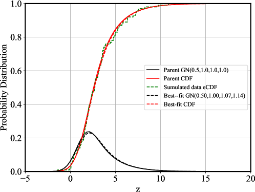
An example of the results of the fit to a simulated dataset is provided in the top panel of Fig. 6.

Figure 6: Top: maximum likelihood estimation of parameters for a overdispersed chi–squared distribution with fixed $\alpha=\nicefrac{{1}}{{2}}$; Bottom: for an exponential–normal distribution with fixed $r=1$.

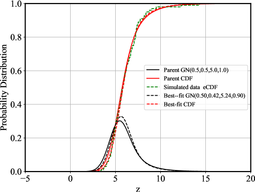
The score equations yield parameter estimates $(\hat{r},\hat{\mu},\hat{\sigma})=(0.42,5.24,0.95)$, with observed information matrix

$$I=\begin{bmatrix}168.65&83.67&21.47\\ 83.67&63.51&-25.44\\ 21.47&-25.44&88.77\\ \end{bmatrix}$$

that has eigenvalues $(215.24,4.57,101.12)$ and $\det(I)=99415.99$. Inversion of this matrix leads to the the observed covariance matrix

$$\epsilon=\begin{bmatrix}0.0502&-0.0802&-0.0351\\ -0.0802&0.1459&0.0612\\ -0.0351&0.0612&0.0373\\ \end{bmatrix}$$

Similar values are obtained for other equivalent simulations.

It is useful to point out the negative correlation that is typically observed between estimates of the $r$ and $\mu$ parameters, and between estimates of the $r$ and $\sigma$ parameters. These correlations are a direct result of, respectively, the expectation and variance of the $Z$ variable, see Property 2. For example, as $r$ increases, $\mu$ must decrease (for a fixed $\alpha$) to maintain the same parent mean; and likewise as $r$ increases, $\sigma^{2}$ must be reduced in value to keep the same parent variance. These negative correlations are therefore expected to apply to all applications in which the three parameters $r,\mu,\sigma^{2}$ are simultaneously estimated from a single set of data.

In applications where the $\alpha=\nicefrac{{1}}{{2}}$ gamma distribution becomes a chi–squared distribution with $\nu=2r\in\mathbb{N}$, it is no longer meaningful to estimate the $r$ parameter via the equations presented in this paper, which assumes the more general case of $r\in\mathbb{R}^{+}$. Instead, the $\nu$ parameter must be held fixed, and a two–parameter estimation can be performed using only the two equations that apply to the $\mu$ and $\sigma$ parameters.

4.3.3 The exponential–normal distribution

When $r=1$, the gamma–normal distribution becomes the exponential–normal distribution discussed in Sec. 3.1. An example of parameter estimation is shown in the bottom panel of Fig. 6, featuring an observed information matrix

$$I=\begin{bmatrix}326.92&-61.54&-16.01\\ -61.54&33.68&-14.02\\ -16.01&-14.02&42.63\\ \end{bmatrix}$$

with eigenvalues $(339.87,11.86,51.50)$ and $\det(I)=207530.90$. The observed covariance matrix is

$$\epsilon=\begin{bmatrix}0.0060&0.0137&0.0068\\ 0.0137&0.0660&0.0268\\ 0.0068&0.0268&0.0348\\ \end{bmatrix}$$

Since $r$ is fixed, there is now a positive correlation between the $(\alpha$, $\mu)$ and the $(\mu$, $\sigma^{2})$ pairs of parameters. This is again in accordance with the mean and variance of the $Z$ variable, as already discussed for the overdispersed chi–squared distribution above.

5 Discussion of certain applications of the gamma–normal  distribution

The gamma–normal distribution may apply to any statistic or random variable that is the sum of independent gamma and normal random variables (one of each), according to its definition (5). It is therefore a general–purpose distribution that is useful for a variety of applications, and it goes beyond the scope of this paper to review all of them. In the following we briefly review and discuss a few possible applications, with emphasis on two categories that are of interest to recent real–data applications.

5.1 Application to noise–signal deconvolution

The gamma–normal distribution was proposed by Plancade et al. (2012) as an extension of the exponential–normal distribution (e.g. Gruskha, 1972; Xie et al., 2009) for the purpose of noise–signal decomposition in the analysis of fluorescence data from biological samples with the Illumina BeadArray technology. In that application, $Z=X+Y$ is the total signal, whereas $X\sim\gamma(\alpha,r)$ is the signal of interest, and $Y\sim N(\mu,\sigma^{2})$ is the background. The gamma–normal model was proposed in response to the lack of a proper fit of the fluorescence data with the exponential–normal model noted by, e.g., Wang and Ye (2012), and current applications of this model rely on a Fast Fourier Transform (FFT) of the convolution. The analytic form (5) is expected to provide a substantial improvement in the analysis of these data both in terms of speed and accuracy.

Similar applications of the gamma–normal distribution can be envisioned for any type of emission that results from the convolution of signal and background, which is a common experimental task. For example, background correction in certain biological data are reviewed by Ritchie et al. (2007), including the exponential–normal distribution that is now generalized by the gamma–normal distribution. Similar background subtraction tasks occur routinely in the physical sciences (see, e.g., Ehlert et al., 2022; Blanton et al., 2011, for applications to astronomy). The gamma–normal distribution could therefore provide a suitable and versatile model for background deconvolution in any application where the two components can be modeled via these continuous distributions.

5.2 Application to hypothesis testing of Poisson regression with systematic errors

Systematic errors in the data, broadly defined as additional sources of error due to errors in measurement or to uncertainties in the underlying model, are a common occurrence in applications (see, e.g., Glosup and Axelrod, 1996; van Dyk and Lyons, 2023, for a review). An open problem for the use of systematic errors in data regression is how those errors affect the goodness–of–fit statistic for integer–valued Poisson data. The goodness–of–fit statistic for the regression of Poisson data to a parametric function, also referred to as the Poisson deviance $D_{P}$, is asymptotically distributed as $\chi^{2}$ in the large–mean regime (e.g., Cameron and Trivedi, 2013; Cash, 1979; Bishop et al., 1975), just as it is for normal data (see Sec. 3.2). In Bonamente (2023), the first author proposed a statistical model to account for systematic errors in the maximum likelihood Poisson regression of certain count data. This model results in a goodness–of–fit statistic $Z=X+Y$ that is now distributed as the sum of the usual $X\sim\chi^{2}(\nu)$ $D_{P}$ statistic and an independent $Y\sim N(\mu,\sigma^{2})$ statistic that models the effects of systematic errors, where $\mu$ and $\sigma^{2}$ can be estimated from the data.

The overdispersed chi–squared distribution $\mathrm{B}(\nu,\mu,\sigma^{2})$ presented in Sec. 3.2 is therefore the relevant distribution of this Poisson goodness–of–fit statistic, under the null hypothesis of the correctness of the parametric model. Table 1 provides the quantiles (i.e., one–sided critical values) of this distribution for selected values of the integer number of degrees of freedom $\nu$ and the overdispersion parameter $\sigma^{2}$. These values are obtained by numerical integration of (13), and can be used for the rejection of the null hypothesis at a given level of significance. Similarly, (13) can also be used to calculate the $p$–value of the regression, via $1-p=F_{\mathrm{B}}(D_{P})$, where $D_{P}$ is the observed value of the fit statistic and $F_{\mathrm{B}}$ denotes the cumulative distribution function.

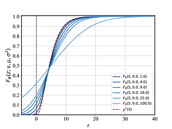
Figure 7 illustrates an important property of the overdispersed chi–squared distribution, namely that quantiles of the $B(\nu,\mu=0,\sigma^{2})$ distribution for $p>0.5$ are larger than those for the corresponding $\chi^{2}(\nu)$ distribution, i.e.,

$$F^{-1}_{B}(p)>F^{-1}_{\chi^{2}}(p),\;\text{ for $p>0.5$}.$$ (20)

For the purpose of hypothesis testing, this means that the addition of the normal distribution (as a model for systematic errors) to the chi–square distribution results in larger critical values, i.e., the presence of systematic errors makes it more difficult to reject the null hypothesis. Moreover, Property 3 shows that in the asymptotic limit of a large number of degrees of freedom, the Poisson deviance is normally distributed, $D_{P}\sim N(\nu+\mu,2\nu+\sigma^{2})$, since the $\chi^{2}(\nu)$ distribution is approximated by a normal distribution with the same mean and variance.

Figure 7: CDF of an overdispersed chi–squared $B(\nu,\mu,\sigma^{2})$ variable for a fiducial value of $\nu$ and $\mu=0$, and for selected values of the overdispersion parameter $\sigma^{2}$.

5.3 Other possible applications

The gamma distribution for integer values of the shape parameter, $r\in\mathbb{N}$, is also known as the Erlang distribution, after A. K. Erlang who used it to model the distribution of time between phone calls (Erlang, 1909). The Erlang distribution can be used to model a variety of counting phenomena that follow from the Poisson process with fixed rate $\alpha$. Accordingly, the addition of a normal distribution can be a simple way to model overdispersion (and optionally a shift in the mean, if $\mu\neq 0$) for such processes.

6 Discussion and conclusions

In this paper, we have first presented key properties of the random variable that results from the sum of an independent gamma variable with rate parameter $\alpha$ and shape parameter $r$, and a normal random variable with mean $\mu$ and variance $\sigma^{2}$. The resulting random variable is referred to as the gamma–normal random variable $\mathrm{GN}(\alpha,r,\mu,\sigma^{2})$, and it features a pdf that can be written in compact form with the aid of parabolic cylinder functions. This new distribution was first proposed by Plancade et al. (2012) for the analysis of certain biological data. Two special cases of this distribution are the exponential–normal distribution obtained for a fixed shape parameter $r=1$, and the overdispersed chi–squared distribution obtained for a fixed rate parameter $\alpha=\nicefrac{{1}}{{2}}$. A key property of the gamma–normal distribution is that the $\mu$ parameter continues to be a simple location parameter (see Property 1) that does not otherwise affect the shape of the distribution, the same as for the normal distribution.

We have then provided analytical expressions for the maximum likelihood score equations, and the observed information matrix $I$ of the gamma–normal distribution. These results were applied to extensive simulated data sets intended to illustrate the methods of parameter estimation for this class of random variables. The results provided in this paper suggest that of the four parameters of the gamma–normal distribution, only three can be identified independently, according to the Rothenberg rank criterion for $\text{E}(I)$ (Rothenberg, 1971). This finding in turn suggests that there may be an alternative reparameterization of the gamma–normal model as a function of three parameters, although such a reparameterization is not obvious to identify. When either the rate or the shape parameter of the gamma distribution is held fixed, the estimation successfully recovers the other three parameters, providing further indication that $\mathrm{rank}(I)=3$ for the gamma–normal distribution in its most general form.

Given the broad use of the two constituting distributions in probability and statistics, the gamma–normal distribution may occur in a wide variety of applications. In particular, the gamma–normal distribution was first proposed for certain biological applications (e.g. Plancade et al., 2012) as a more general method to fit certain data that were not successfully modeled with the exponential–normal distribution (e.g. Gruskha, 1972; Golubev, 2010). It is hoped that the present investigation, with the derivation of analytic expressions for the maximum likelihood estimation, will benefit such applications.

The overdispersed chi–squared distribution, on the other hand, is the parent model for the goodness–of–fit of certain Poisson data that feature systematic errors (e.g. Bonamente, 2023). In that class of applications, the main difference with the positively–supported $\chi^{2}$ distribution is a tail of negative values that becomes more prominent as $\sigma$ increases, for a fixed value of $\mu$, and it is a consequence of the convolution with the real–valued normal distribution that models the presence of systematic errors. The paper has also provided critical values for the $B(\nu,\mu=0,\sigma^{2})$ for representative values of the $\nu$ and $\sigma^{2}$ parameters that can be used for hypothesis testing.  Thanks to the translation property of the gamma–normal distribution, these quantiles can be used also for applications with $\mu\neq 0$.

Appendix A Distributions and functions of interest

The probability distribution function (pdf) of a gamma random variable $X\sim\gamma(\alpha,r)$ is defined as

$$f_{\gamma}(x)=\dfrac{\alpha(\alpha x)^{r-1}}{\Gamma(r)}e^{-\alpha x}$$ (21)

with $\alpha,r$ positive real numbers, and $x\geq 0$. The parameter $\alpha$ is referred to as the rate parameter (and $1/\alpha$ as the scale parameter), and $r$ is the shape parameter.

The pdf of an exponential random variable $X\sim\mathrm{Exp}(\alpha)$ has a probability distribution

$$f_{E}(x)=\alpha e^{-\alpha x}$$ (22)

where $\alpha$ is known as the rate parameter, and $1/\alpha$ as the scale parameter.

The pdf of a chi–squared random variable $X\sim\chi^{2}(\nu)$ is

$$f_{\chi^{2}}(x)=\left(\dfrac{1}{2}\right)^{\nu/2}\dfrac{1}{\Gamma(\nu/2)}e^{-x/2}x^{\nu/2-1}$$ (23)

with $\nu\in\mathbb{R}^{+}$. In many statistical applications, $\nu\in\mathbb{N}$ signifies the number of degrees of freedom of the distribution.

The error function is defined as

$$\text{erf}(x)=\dfrac{2}{\sqrt{\pi}}\int_{0}^{\infty}e^{-t^{2}}dt.$$ (24)

Let $F(x)$ be the cumulative distribution function of a standard normal variable $X\sim N(0,1)$. Then it is true that

$$F(\sqrt{2}\,x)=\dfrac{1}{2}\left(1+\text{erf}(x)\right)$$ (25)

and

$$F(-\sqrt{2}\,x)=\dfrac{1}{2}\left(1-\text{erf}(x)\right).$$ (26)

The latter equation can be used to show that the pdf of the exponential–normal distribution as given by (11) is equivalent to Eq. 3 of Xie et al. (2009).

The following recursion formulas apply to the parabolic cylinder functions (see 9.247, Gradshteyn and Ryzhik, 2007):

$$\begin{cases}D_{p+1}(z)-zD_{p}(z)+pD_{p-1}(z)=0\\[10.0pt] \dfrac{d}{dz}D_{p}(z)=\dfrac{1}{2}zD_{p}(z)-D_{p+1}(z)\\[10.0pt] \dfrac{d}{dz}D_{p}(z)=-\dfrac{1}{2}zD_{p}(z)+pD_{p-1}(z)\end{cases}$$ (27)

In particular, given the restriction that the index of the parabolic cylinder function is negative, the last equation of (27) applies when $p-1<0$. With our use of the parameter $r=-p$, this restriction translates to $r>-1$, which is always satisfied in our application. Therefore the equation of choice to express the derivative of the parabolic cylinder functions with respect to its argument, via the parabolic functions themselves, becomes

$$\dfrac{d}{d\zeta}D_{-r}(\zeta)=-\dfrac{\zeta}{2}D_{-r}(\zeta)-rD_{-r-1}(\zeta).$$ (28)

Appendix B Equations for maximum–likelihood estimation with the gamma–normal distribution

Consider $N$ iid measurements $z_{i}\sim\mathrm{GN}(\theta)$, with $\theta=(\alpha,r,\mu,\sigma)$ the four parameters of the gamma–normal distribution. The log–likelihood is

$$\mathcal{L}=\sum_{i=1}^{N}\ln f_{\mathrm{GN}}(z_{i}/\theta)$$ (29)

with

$$\ln f_{\mathrm{GN}}(z_{i}/\theta)=\ln\left(\dfrac{\alpha^{r}\sigma^{r-1}}{\sqrt{2\pi}}\right)+\ln D_{-r}(\zeta)+\ln E(z),$$ (30)

where $\zeta(z)$ is given by (6) and $\ln E(z)$ by (7).

B.1 The score function

The maximum likelihood estimates $\hat{\theta}$ are given by setting the score functions to zero, $d\mathcal{L}/d\theta|_{\hat{\theta}}=0$, and then solving. We will consider separately the score functions for the parameters $\alpha,\mu,\sigma$, and then the one for the parameter $r$ which occurs as the index of the parabolic cylinder function.

(A) For $\theta=(\alpha,\mu,\sigma)$, the derivatives of the log–likelihood are obtained from derivatives of elementary functions,

$$\begin{cases}\dfrac{d\zeta}{d\theta}=\left(\sigma,\dfrac{1}{\sigma},\alpha-\dfrac{\mu-z}{\sigma^{2}}\right)\\[10.0pt] \dfrac{d\ln E(z)}{d\theta}=\left(0,\dfrac{z-\mu}{\sigma^{2}},\dfrac{(z-\mu)^{2}}{\sigma^{3}}\right)+\dfrac{\zeta}{2}\left(\dfrac{d\zeta}{d\theta}\right),\end{cases}$$ (31)

and from the derivative of the parabolic cylinder function with respect to its argument, according to the bottom equation of (27), which is always satisfied in this application:

$$D_{-r}^{^{\prime}}(\zeta)=-\dfrac{1}{2}\zeta D_{-r}(\zeta)-rD_{-r-1}(\zeta),\text{ if $r\geq-1$}.$$ (32)

Therefore, for the parameters $\theta=(\alpha,\mu,\sigma)$, the three score functions for the $i$–th datum are summarized as

$$\left.\dfrac{d\ln f_{\mathrm{GN}}(z)}{d\theta}\right|_{z_{i}}=\left(\dfrac{r}{\alpha},0,\dfrac{r-1}{\sigma}\right)+\dfrac{D_{-r}^{^{\prime}}(\zeta_{i})}{D_{-r}(\zeta_{i})}\,\left.\dfrac{d\zeta}{d\theta}\right|_{z_{i}}+\left.\dfrac{d\ln E(z)}{d\theta}\right|_{z_{i}}.$$ (33)

(B) For $\theta=r$, a derivative of $D_{-r}(\zeta)$ with respect to $r$ is required. With

$$D_{-r}(z)=\dfrac{e^{-z^{2}/4}}{\Gamma(r)}\int_{0}^{\infty}e^{-xz-x^{2}/2}x^{r-1}dx\equiv\dfrac{e^{-z^{2}/4}}{\Gamma(r)}A(z,r),$$ (34)

the problem becomes that of finding the derivatives of $A(z,r)$ and $\Gamma(r)$ with respect to r. First, recall that

$$\dfrac{d\Gamma(r)}{dr}=\psi(r)\Gamma(r)$$

where $\psi(r)$ is the digamma function. For $A(z,r)$, we may use the Leibnitz rule to obtain

$$\dfrac{\partial A(z,r)}{\partial r}=\int_{0}^{\infty}e^{-xz-x^{2}/2}x^{r-1}\ln x\,dx\equiv A_{r}(z,r)$$ (35)

which does not appear to have a simpler analytic form. Therefore

$$\dfrac{\partial}{\partial r}\ln D_{-r}(\zeta)=\left.\dfrac{A_{r}(\zeta,r)}{A(\zeta,r)}\right|_{z_{i}}-\psi(r),$$ (36)

and the score function for $\theta=r$ is given by

$$\left.\dfrac{\partial\ln f_{\mathrm{GN}}(z)}{\partial r}\right|_{z_{i}}=(\ln\alpha+\ln\sigma)+\left.\dfrac{A_{r}(\zeta,r)}{A(\zeta,r)}\right|_{z_{i}}-\psi(r).$$ (37)

Note how the factorization of (34) is convenient for the logarithmic derivative.

Accordingly, the score equations for $\hat{\theta}_{j}$, for $j=1,\dots,4$, are

$$\dfrac{\partial\mathcal{L}}{\partial\theta_{j}}=\sum_{i=1}^{N}\left.\dfrac{\partial\ln f_{\mathrm{GN}}(z)}{\partial\theta_{j}}\right|_{z_{i},\hat{\theta}}=0,$$ (38)

with derivatives given by (33) and (37). Eq. 38 is a system of four nonlinear equations that requires numerical solution for $\hat{\theta}=(\hat{\alpha},\hat{r},\hat{\mu},\hat{\sigma})$. When evaluating the sum of the scores over $N$ iid measurements, it is convenient to define the following sums:

$$\begin{cases}Z_{1}=\dfrac{1}{N}\sum\limits_{i=1}^{N}(\mu-z_{i})=(\mu-\overline{z}),\;Z_{2}=\dfrac{1}{N}\sum\limits_{i=1}^{N}(\mu-z_{i})^{2};\\[10.0pt] S=\dfrac{1}{N}\sum\limits_{i=1}^{N}\left(\dfrac{D_{-r}^{\prime}(\zeta_{i})}{D_{-r}(\zeta_{i})}\right),\;S_{\mu}=\dfrac{1}{N}\sum\limits_{i=1}^{N}\left(\dfrac{D_{-r}^{\prime}(\zeta_{i})}{D_{-r}(\zeta_{i})}\right)(\mu-z_{i});\\[15.0pt] T=\dfrac{1}{N}\sum\limits_{i=1}^{N}\left(\dfrac{A_{r}(\zeta_{i},r)}{A(\zeta_{i},r)}\right).\\[10.0pt] \end{cases}$$ (39)

B.2 The information matrix

The observed information matrix is the symmetric $4\times 4$ matrix

$$I=-\dfrac{\partial^{2}\mathcal{L}}{\partial\theta\partial\theta^{T}}=-\dfrac{\partial}{\partial\theta}\left(\dfrac{\partial\mathcal{L}}{\partial\theta^{T}}\right)=-\sum_{i=1}^{N}\dfrac{\partial^{2}}{\partial\theta\partial\theta^{T}}\ln f_{\mathrm{GN}}(z_{i}/\theta)$$

with $\theta=(\alpha,r,\mu,\sigma)$ and $T$ denoting the transpose of a vector, and therefore it is the sum over the $N$ measurements of the second–order partial derivatives of the logarithm of the gamma–normal density.

The second–order derivatives can be calculated starting from (33) and (37). The derivatives with respect to $r$ (the index of the parabolic cylinder functions) and with respect to the other parameters that appear in the argument $\zeta=\zeta(\alpha,\mu,\sigma)$ are calculated separately, given that the recursion formulas (32) only apply to derivatives with respect to the argument $\zeta$. The second–order derivatives require the following functions:

$$\dfrac{d}{d\zeta}\left[\dfrac{D_{-r}^{\prime}(\zeta)}{D_{-r}(\zeta)}\right]=\dfrac{d}{d\zeta}\left[\dfrac{d}{d\zeta}\ln D_{-r}(\zeta)\right]=\dfrac{D_{-r}^{\prime\prime}(\zeta)D_{-r}(\zeta)-D_{-r}^{\prime}(\zeta)^{2}}{D_{-r}(\zeta)^{2}}$$ (40)

where the recursion equations (32) can be used to evaluate the first–order derivatives $D_{-r}^{\prime}(\zeta)$ as a function of the parabolic cylinder functions, see (32). Moreover,

$$D_{-r}^{\prime\prime}(\zeta)\equiv\dfrac{\partial}{\partial\zeta}D_{-r}^{\prime}(\zeta)=-\dfrac{1}{2}D_{-r}(\zeta)-\dfrac{\zeta}{2}D_{-r}^{\prime}(\zeta)-rD_{-r-1}^{\prime}(\zeta)\;\text{ for $r\geq-1$}$$ (41)

where the recursion equations (32) were used. Given that the derivatives of the parabolic cylinder functions are readily available, it is not necessary to use the recursion equations again in (41) in order to eliminate the derivatives.

For the derivatives with respect to $r$, the following results are needed. First,

$$\dfrac{\partial}{\partial r}\left[\dfrac{D_{-r}^{\prime}(\zeta)}{D_{-r}(\zeta)}\right]=\dfrac{\dfrac{d}{dr}D_{-r}^{\prime}(\zeta)\cdot D_{-r}(\zeta)-\dfrac{d}{dr}D_{-r}(\zeta)\cdot D_{-r}^{\prime}(\zeta)}{D_{-r}(\zeta)^{2}}$$ (42)

where the derivatives with respect to $r$ are given by

$$\begin{cases}\dfrac{d}{dr}D_{-r}(\zeta)=D_{-r}(\zeta)\left(\dfrac{A_{r}(\zeta,r)}{A(\zeta,r)}-\psi(r)\right)\\[10.0pt] \dfrac{d}{dr}D_{-r}^{\prime}(\zeta)=-\dfrac{1}{2}\zeta\dfrac{d}{dr}D_{-r}(\zeta)-D_{-r-1}(\zeta)-r\dfrac{d}{dr}D_{-r-1}(\zeta)\;\text{ for $r\geq-1$}\end{cases}$$

and therefore they can all be expressed as functions of the parabolic cylinder functions and the function $A_{r}(\zeta,r)$ that was defined in (35).

The derivatives with respect to $r$ of the two functions of $r$ in (37) can be evaluated as

$$\dfrac{d}{dr}\left(\dfrac{A_{r}(\zeta,r)}{A(\zeta,r)}\right)=\dfrac{A_{rr}(\zeta,r)A(\zeta,r)-A_{r}(\zeta,r)^{2}}{A(\zeta,r)^{2}}$$ (43)

which requires the following additional integral:

$$\dfrac{d}{dr}A_{r}(\zeta,r)=\int_{0}^{\infty}e^{-xz-x^{2}/2}x^{r-1}(\ln x)^{2}\,dx\equiv A_{rr}(z,r).$$ (44)

The cross–derivative of $A_{r}/A$ with respect to $\zeta$ can be related to the cross–derivative of $\partial/\partial\zeta\ln D_{-r}(\zeta)$ with the use of (36) and a change in the order of the derivatives:

$$\dfrac{\partial}{\partial\zeta}\left(\frac{A_{r}}{A}\right)=\dfrac{\partial}{\partial\zeta}\left(\dfrac{\partial}{\partial r}\ln D_{-r}(\zeta)\right)=\dfrac{\partial}{\partial r}\left(\dfrac{\partial}{\partial\zeta}\ln D_{-r}(\zeta)\right).$$

Finally, the derivative of the digamma function is a polygamma function of order 1, $\psi_{1}(r)$,

$$\dfrac{d}{dr}\psi(r)=\psi^{\prime}(r)=\psi_{1}(r).$$

The second–derivatives matrix $I_{\star}=(I_{1\,\star}^{T},I_{2\,\star}^{T},I_{3\,\star}^{T},I_{4\,\star}^{T})$ for one observation of the gamma–normal distribution is as follows:

$$I_{1\,\star}= \dfrac{d}{d\theta}\left(\dfrac{\partial}{\partial\alpha}\ln f_{\mathrm{GN}}(z_{i})\right)=\left(-\dfrac{r}{\alpha^{2}}+\dfrac{d}{d\alpha}\left(\dfrac{D_{-r}^{\prime}(\zeta)}{D_{-r}(\zeta)}\right)\sigma+\dfrac{\sigma^{2}}{2},\dfrac{1}{\alpha}+\sigma\dfrac{\partial}{\partial r}\left(\dfrac{D_{-r}^{\prime}(\zeta)}{D_{-r}(\zeta)}\right),\right.$$ (45)

$$\left.\dfrac{d}{d\mu}\left(\dfrac{D_{-r}^{\prime}(\zeta)}{D_{-r}(\zeta)}\right)\sigma+\dfrac{1}{2},\dfrac{d}{d\sigma}\left(\dfrac{D_{-r}^{\prime}(\zeta)}{D_{-r}(\zeta)}\right)\sigma+\left(\dfrac{D_{-r}^{\prime}(\zeta)}{D_{-r}(\zeta)}\right)+\alpha\sigma\right)$$

$$I_{2\,\star}= \dfrac{d}{d\theta}\left(\dfrac{\partial}{\partial r}\ln f_{\mathrm{GN}}(z_{i})\right)=\left(\dfrac{1}{\alpha}+\dfrac{d}{d\alpha}\left[\dfrac{A_{r}(\zeta,r)}{A(\zeta,r)}\right],\dfrac{d}{dr}\left[\dfrac{A_{r}(\zeta,r)}{A(\zeta,r)}-\psi(r)\right],\right.$$ (46)

$$\left.\dfrac{d}{d\mu}\left[\dfrac{A_{r}(\zeta,r)}{A(\zeta,r)}\right],\dfrac{1}{\sigma}\dfrac{d}{d\sigma}\left[\dfrac{A_{r}(\zeta,r)}{A(\zeta,r)}\right]\right)$$

$$I_{3\,\star}= \dfrac{d}{d\theta}\left(\dfrac{\partial}{\partial\mu}\ln f_{\mathrm{GN}}(z_{i})\right)=$$ (47)

$$\left(\dfrac{d}{d\alpha}\left(\dfrac{D_{-r}^{\prime}(\zeta)}{D_{-r}(\zeta)}\right)\dfrac{1}{\sigma}+\dfrac{1}{2},\dfrac{d}{dr}\left(\dfrac{D_{-r}^{\prime}(\zeta)}{D_{-r}(\zeta)}\right)\dfrac{1}{\sigma},\dfrac{d}{d\mu}\left(\dfrac{D_{-r}^{\prime}(\zeta)}{D_{-r}(\zeta)}\right)\dfrac{1}{\sigma}-\dfrac{1}{2\sigma^{2}},\right.$$

$$\left.\dfrac{d}{d\sigma}\left(\dfrac{D_{-r}^{\prime}(\zeta)}{D_{-r}(\zeta)}\right)\dfrac{1}{\sigma}-\dfrac{1}{\sigma^{2}}\left(\dfrac{D_{-r}^{\prime}(\zeta)}{D_{-r}(\zeta)}\right)-\dfrac{z-\mu}{\sigma^{3}}-\dfrac{\alpha}{\sigma}\right)$$

$$I_{4\,\star}= \dfrac{d}{d\theta}\left(\dfrac{\partial}{\partial\sigma}\ln f_{\mathrm{GN}}(z_{i})\right)=\left(\dfrac{d}{d\alpha}\left(\dfrac{D_{-r}^{\prime}(\zeta)}{D_{-r}(\zeta)}\right)\left(\alpha-\dfrac{\mu-z}{\sigma^{2}}\right)+\left(\dfrac{D_{-r}^{\prime}(\zeta)}{D_{-r}(\zeta)}\right)+\alpha\sigma,\right.$$ (48)

$$\dfrac{1}{\sigma}+\dfrac{d}{dr}\left(\dfrac{D_{-r}^{\prime}(\zeta)}{D_{-r}(\zeta)}\right)\left(\alpha-\dfrac{\mu-z}{\sigma^{2}}\right),\dfrac{d}{d\mu}\left(\dfrac{D_{-r}^{\prime}(\zeta)}{D_{-r}(\zeta)}\right)\left(\alpha-\dfrac{\mu-z}{\sigma^{2}}\right)$$

$$-\dfrac{1}{\sigma^{2}}\left(\dfrac{D_{-r}^{\prime}(\zeta)}{D_{-r}(\zeta)}\right)+\dfrac{\mu-z}{\sigma^{3}},$$

$$-\dfrac{r-1}{\sigma^{2}}+\dfrac{d}{d\sigma}\left(\dfrac{D_{-r}^{\prime}(\zeta)}{D_{-r}(\zeta)}\right)\left(\alpha-\dfrac{\mu-z}{\sigma^{2}}\right)+\left(\dfrac{D_{-r}^{\prime}(\zeta)}{D_{-r}(\zeta)}\right)\dfrac{2(\mu-z)}{\sigma^{3}}+\dfrac{\alpha}{2}$$

$$\left.-\dfrac{3}{2}\dfrac{(z-\mu)^{2}}{\sigma^{4}}\right)$$

When evaluating the information matrix for $N$ iid measurements, as in (19), all the functions in (45)–(48) must be evaluated at the $i$–th measurement $\zeta(z_{i})$ according to (6).

The following sum over the $N$ data points must be evaluated to calculate the information matrix:

$$\begin{cases}S_{\zeta}=\dfrac{1}{N}\sum\limits_{i=1}^{N}\left[\dfrac{\partial}{\partial\zeta}\left(\dfrac{D_{-r}^{\prime}(\zeta_{i})}{D_{-r}(\zeta_{i})}\right)\right]=\dfrac{\partial S}{\partial\zeta},\\[10.0pt] S_{r}=\dfrac{1}{N}\sum\limits_{i=1}^{N}\left[\dfrac{\partial}{\partial r}\left(\dfrac{D_{-r}^{\prime}(\zeta_{i})}{D_{-r}(\zeta_{i})}\right)\right]=\dfrac{\partial S}{\partial r},\\[10.0pt] S_{r,\mu}=\dfrac{1}{N}\sum\limits_{i=1}^{N}\left[\dfrac{\partial}{\partial r}\left(\dfrac{D_{-r}^{\prime}(\zeta_{i})}{D_{-r}(\zeta_{i})}\right)(\mu-z_{i})\right],\\[10.0pt] T_{r}=\dfrac{1}{N}\sum\limits_{i=1}^{N}\left[\dfrac{\partial}{\partial r}\left(\dfrac{A_{r}(\zeta_{i},r)}{A(\zeta_{i},r)}\right)\right]=\dfrac{\partial T}{\partial r},\\[10.0pt] S_{\zeta,\mu}=\dfrac{1}{N}\sum\limits_{i=1}^{N}\left[\dfrac{\partial}{\partial\zeta}\left(\dfrac{D_{-r}^{\prime}(\zeta_{i})}{D_{-r}(\zeta_{i})}\right)\right](\mu-z_{i}),\\[10.0pt] S_{\zeta,\mu^{2}}=\dfrac{1}{N}\sum\limits_{i=1}^{N}\left[\dfrac{\partial}{\partial\zeta}\left(\dfrac{D_{-r}^{\prime}(\zeta_{i})}{D_{-r}(\zeta_{i})}\right)\right](\mu-z_{i})^{2}.\\[10.0pt] \end{cases}$$ (49)

Appendix C Numerical methods for maximum likelihood estimation

C.1 Iterative solution of the score equations

Numerical solution of the score equations (15) was performed with the least_squares function available from scipy in python. The function iteratively seeks a solution of the score equations, starting at a point in parameter space $\theta$ that was set close to the parent values of the distribution. Although the Jacobian of the system of equations is available as the second–order derivatives of the log likelihood in (19), we opted for a numerical estimation via the 2-point optional parameter.

C.2 The ratio $D^{\prime}_{-r}(\zeta)/D_{-r}(\zeta)$ and its derivative with respect to $\zeta$

A numerical challenge to finding the solution of the score equations is the large value of the parabolic cylinder functions $D_{-r}(\zeta)$ and its derivative with respect to the argument $\zeta$, i.e. $D^{\prime}_{-r}(\zeta)$, which are both available in the same package via the pbdv function. In fact, as illustrated in Fig. 2, the parabolic cylinder functions diverge as $z$ increases, and therefore as $\zeta$ decreases according to (6); similar asymptotic divergence occurs for the derivative, which is related to the function itself via the recursion relations (27). Accordingly, datasets with large values of the $Z$ variable need to be handled with care due to possible overflow problems.

Fortunately, it is possible to overcome these problems for most applications. We suggest two possible avenues.
(a) According to the translation property of the gamma–normal distribution (Property 1), the data can be shifted to lower values by a fixed constant. This constant is then added to the $\mu$ parameter estimate.
(b) The scores and the information matrix depend only on logarithmic derivatives, i.e., the ratios of the derivatives to the parabolic cylinder functions themselves, see the sum terms $S$ and $S_{\zeta}$ in (39) and (49). Both ratios $D^{\prime}_{-r}(\zeta)/D_{-r}(\zeta)$ and $d/d\zeta(D^{\prime}_{-r}(\zeta)/D_{-r}(\zeta))$ have values that are close to unity, in a large range of the variable $\zeta$. In particular, we observe that

$$\lim\limits_{\zeta\to\infty}\;\dfrac{d}{d\zeta}\left(\dfrac{D^{\prime}_{-r}(\zeta)}{D_{-r}(\zeta)}\right)=\dfrac{1}{2},$$

which can be used for the sums $S_{\zeta}$, $S_{\zeta,\mu}$ and $S_{\zeta,\mu^{2}}$ in the asymptotic limit of a large argument. There are also a number of asymptotic expansions of the parabolic cylinder function (see Sec. 9.246 of Gradshteyn and Ryzhik, 2007) that can be used to approximate the sums $S$ and $S_{\mu}$ for large values of their argument. It is therefore possible to use asymptotic expressions for the ratios in the sums (39) and (49) to bypass the direct evaluation of the parabolic cylinder functions, and to avoid overflow problems. Those approximations are not discussed in this paper.

C.3 The ratio $A_{r}(\zeta,r)/A(\zeta,r)$ and its derivative with respect to $r$

The derivatives of the parabolic cylinder functions with respect to the index $r$ lead to the integrals $A_{r}$ and $A_{rr}$ that are evaluated according to the Leibnitz rule; see (35) and (44). Those integrations can be performed via standard numerical integration methods, and they diverge for large negative values of the $Z$ variable, and accordingly for large positive values of the $\zeta$ argument. Fortunately, the ratio $A_{r}(\zeta,r)/A(\zeta,r)$ remains a small number in the vicinity of zero for a large range of the $\zeta$ and $r$ parameters. The same applies to the ratio $d/dr(A_{r}(\zeta,r)/A(\zeta,r))$ which appears in $T_{r}$. Therefore the same strategies suggested in Sec. C.2 apply also for these ratios.

References

- Amemiya (1985) Amemiya, T., 1985. Advanced Econometrics. Harvard University Press.
- Bernardo and Smith (2000) Bernardo, J.M., Smith, A.F.M., 2000. Bayesian Theory.
- Bishop et al. (1975) Bishop, Y., Fienberg, S., Holland, P., 1975. Discrete Multivariate Analysis: Theory and Practice : Yvonne M.M. Bishop, Stephen E. Fienberg and Paul W. Holland. Massachusetts Institute of Technology Press. URL: https://books.google.com/books?id=apQDnwEACAAJ.
- Blanton et al. (2011) Blanton, M.R., Kazin, E., Muna, D., Weaver, B.A., Price-Whelan, A., 2011. Improved background subtraction for the sloan digital sky survey images. The Astronomical Journal 142, 31. URL: https://dx.doi.org/10.1088/0004-6256/142/1/31, doi:10.1088/0004-6256/142/1/31.
- Bonamente (2023) Bonamente, M., 2023. Systematic errors in the maximum-likelihood regression of Poisson count data: introducing the overdispersed 2 distribution. Monthly Notices of the Royal Astronomical Society 522, 1987–2001. doi:10.1093/mnras/stad463, arXiv:2302.04011.
- Cameron and Trivedi (2013) Cameron, C., Trivedi, P., 2013. Regression Analysis of Count Data (Second Ed.). Cambridge University Press.
- Carr et al. (2009) Carr, P., Madan, D., Smith, R., 2009. Saddle point methods for option pricing. The Journal of Computational Finance 13, 49–61. doi:10.21314/JCF.2009.198.
- Cash (1979) Cash, W., 1979. Parameter estimation in astronomy through application of the likelihood ratio. Astrophys. J. 228, 939.
- Delley (1985) Delley, R., 1985. Series for the exponentially modified Gaussian peak shape. Analytical Chemistry 57, 388–388. doi:10.1021/ac00279a094.
- van Dyk and Lyons (2023) van Dyk, D., Lyons, L., 2023. How to incorporate systematic effects into parameter determination. arXiv:2306.05271.
- Ehlert et al. (2022) Ehlert, S., Chen, C.T., Swartz, D., Hickox, R.C., Lutovinov, A., Semena, A., Krivonos, R., Shtykovsky, A., Tkachenko, A., 2022. A probabilistic method of background removal for high energy astrophysics data. Monthly Notices of the Royal Astronomical Society 515, 5185–5197. URL: https://doi.org/10.1093/mnras/stac2072, doi:10.1093/mnras/stac2072, arXiv:https://academic.oup.com/mnras/article-pdf/515/4/5185/45472367/stac2072.pdf.
- Erlang (1909) Erlang, A., 1909. The theory of probabilities and telephone conversations. Nyt Tidsskrift for Matematik 20, 33.
- Fisher (1966) Fisher, F.M., 1966. The Identification Problem in Econometrics. McGraw–Hill, New York.
- Fisher (1924) Fisher, R., 1924. On a distribution yielding the error functions of several well known statistics. Proc. Int. Congr. Math. 2, 805–813.
- Fisher (1925) Fisher, R., 1925. Statistical Methods for Research Workers. Oliver and Boyd, Edinburgh.
- Glosup and Axelrod (1996) Glosup, J., Axelrod, M., 1996. Systematic error revisited.
- Golubev (2010) Golubev, A., 2010. Exponentially modified Gaussian (EMG) relevance to distributions related to cell proliferation and differentiation. Journal of Theoretical Biology 262, 257–266. doi:10.1016/j.jtbi.2009.10.005.
- Gradshteyn and Ryzhik (2007) Gradshteyn, I.S., Ryzhik, I.M., 2007. Table of integrals, series, and products. Seventh ed., Elsevier/Academic Press, Amsterdam. Translated from the Russian, Translation edited and with a preface by Alan Jeffrey and Daniel Zwillinger, With one CD-ROM (Windows, Macintosh and UNIX).
- Gruskha (1972) Gruskha, E., 1972. Characterization of exponentially modified Gaussian peaks in chromatography. Analytical chemistry 44, 1733–1738.
- Helmert (1876) Helmert, F., 1876. Die genauigkeit der formel von peters zur berechnung des wahrscheinlichen fehlers director beobachtungen gleicher genauigkeit. Astron. Nachr. 88, 192–218.
- Hogg et al. (2023) Hogg, R., Tanis, E., Zimmerman, D., 2023. Probability and Statistical Inference. Pearson, Tenth Edition.
- Kalambet et al. (2011) Kalambet, Y., Kozmin, Y., Mikhailova, K., Nagaev, I., Tikhonov, P., 2011. Reconstruction of chromatographic peaks using the exponentially modified Gaussian function. Journal of Chemometrics 25, 352 – 356. doi:10.1002/cem.1343.
- Karas and Svoboda (2013) Karas, P., Svoboda, D., 2013. Algorithms for efficient computation of convolution, in: Ruiz, G., Michell, J.A. (Eds.), Design and Architectures for Digital Signal Processing. IntechOpen, Rijeka. chapter 8. URL: https://doi.org/10.5772/51942, doi:10.5772/51942.
- Kendall and Stuart (1979) Kendall, M., Stuart, A., 1979. The Advanced Theory of Statistics. Vol.2: Inference and Relationship. London: Griffin, 1979, 4th ed.
- Miller (1952) Miller, J.C.P., 1952. On the choice of standard solutions to Weber’s equation. Proc. Cambridge Philos. Soc. 48, 428–435. doi:10.1017/S03050041000272821.
- Palmer et al. (2011) Palmer, E.M., Horwitz, T., Torralba, A., 2011. What are the shapes of response time distributions in visual search? Journal of experimental psychology: Human perception and performance 37, 58–71.
- Pearson (1900) Pearson, K., 1900. On the criterion that a given system of deviations from the probable in the case of a correlated system of variables is such that it can be reasonably supposed to have arisen from random sampling. The London, Edinburgh, and Dublin Philosophical Magazine and Journal of Science 50, 157–175. doi:10.1080/14786440009463897, arXiv:https://doi.org/10.1080/14786440009463897.
- Plancade et al. (2012) Plancade, S., Rozenholc, Y., Lund, E., 2012. Generalization of the normal-exponential model: exploration of a more accurate parametrisation for the signal distribution on Illumina BeadArrays. BMC Bioinformatics 329.
- Ritchie et al. (2007) Ritchie, M.E., Silver, J., Oshlack, A., Holmes, M., Diyagama, D., Holloway, A., Smyth, G.K., 2007. A comparison of background correction methods for two-colour microarrays. Bioinformatics 23, 2700–2707. URL: https://doi.org/10.1093/bioinformatics/btm412, doi:10.1093/bioinformatics/btm412.
- Rothenberg (1971) Rothenberg, T.J., 1971. Identification in parametric models. Econometrica 39, 577–591. URL: http://www.jstor.org/stable/1913267.
- Sprott (1983) Sprott, D.A., 1983. Estimating the parameters of a convolution by maximum likelihood. Journal of the American Statistical Association 78, 457–460. doi:10.1080/01621459.1983.10477994.
- Wald (1950) Wald, A., 1950. Note on the identification of economic relations. Statistical inference in dynamic economic models 10, 238–244.
- Wang and Ye (2012) Wang, X.F., Ye, D., 2012. The effects of error magnitude and bandwidth selection for deconvolution with unknown error distribution. Journal of nonparametric statistics 24, 153–167. doi:10.1080/10485252.2011.647024.
- Weber (1869) Weber, H., 1869. Ueber die integration der partiellen differentialgleichung:. Mathematische Annalen 1, 1–36. URL: http://eudml.org/doc/156394.
- Whittaker (1902) Whittaker, E.T., 1902. On the functions associated with the parabolic cylinder in harmonic analysis. Proc. London Math. Soc. 35, 417–427. doi:10.1112/plms/s1-35.1.417.
- Xie et al. (2009) Xie, Y., Wang, X., Story, M., 2009. Statistical methods of background correction for Illumina BeadArray data. Bioinformatics 25, 751–757.