Robustness to Subpopulation Shift with Domain Label Noise via Regularized Annotation of Domains

Abstract

Existing methods for last layer retraining that aim to optimize worst-group accuracy (WGA) rely heavily on well-annotated groups in the training data. We show, both in theory and practice, that annotation-based data augmentations using either downsampling or upweighting for WGA are susceptible to domain annotation noise, and in high-noise regimes approach the WGA of a model trained with vanilla empirical risk minimization. We introduce Regularized Annotation of Domains (RAD) in order to train robust last layer classifiers without the need for explicit domain annotations. Our results show that RAD is competitive with other recently proposed domain annotation-free techniques. Most importantly, RAD outperforms state-of-the-art annotation-reliant methods even with only 5% noise in the training data for several publicly available datasets.

1 Introduction

Last-layer retraining (LLR) has emerged as a method for utilizing embeddings from pretrained models to quickly and efficiently learn classifiers in new domains or for new tasks. Because only the linear last layer is retrained, LLR allows transferring to new domains/tasks with much fewer examples than would be required to train a deep network from scratch. One promising use of LLR is to retrain deep models with a focus on fairness or robustness, and because data is frequently made up of distinct subpopulations (oft referred to as groups which we take as a tuple of class and domain labels) (Yang et al., 2023), ensuring both fairness between subpopulations and robustness to shifts among subpopulations remains an important problem.

One way to be robust to these types of shifts and/or to be fair across groups is to optimize for the accuracy of the group that achieves the lowest accuracy, i.e., the worst-group accuracy (WGA). WGA thus presents a lower bound on the overall accuracy of a classifier under any subpopulation shift, thereby assuring that all groups are well classified.

State-of-the-art (SOTA) methods for optimizing WGA generally modify either the distribution of the training data (Kirichenko et al., 2023; Giannone et al., 2021; LaBonte et al., 2023) or the training loss (Arjovsky et al., 2019; Liu et al., 2021; Sagawa et al., 2020; Qiu et al., 2023) in order to account for imbalance amongst groups and successfully learn a classifier which is fair across groups. All of these methods additionally use some form of implicit or explicit regularization in the retraining step to limit overfitting to either the group imbalances or the spuriously correlated features in the training data. Kirichenko et al. (2023) argue that strong $\ell_{1}$ regularization plus data augmentation helps to learn “core features,” those which are correlated with the label for all examples. One can instead use regularization without data augmentation to learn spurious features explicitly, in which case misclassified examples can be viewed as belonging to the minority groups. This allows us to avoid explicit use of group annotations.

We examine two representative data augmentation methods, namely downsampling (Kirichenko et al., 2023; LaBonte et al., 2023) and upweighting (Idrissi et al., 2022; Liu et al., 2021; Qiu et al., 2023) which achieve SOTA WGA with simple modifications to the data and loss, respectively. In the simplest setting, each of these methods requires access to correctly annotated groups in order to balance the contribution of each group to the loss. In practice, group annotations are often noisy (Wei et al., 2022), which can be caused by either domain noise, label noise, or both. Label noise generally affects classifier training and data augmentation, making analysis more challenging. We consider only domain noise so that we can compare with existing methods enhancing WGA. Furthermore, focusing on domain noise presents a stepping stone to analyzing group noise in general.

1.1 Our Contributions

We present theoretical guarantees on the WGA under domain noise when modeling last layer representations as Gaussian mixtures. We show that both DS and UW achieve identical WGA and degrade significantly with an increasing percentage of symmetric domain noise, in the limit degrading to the performance of ERM. This is also confirmed with numerical experiments for a synthetic Gaussian mixture dataset modeling latent representations.

Our key contribution is a two-step methodology involving:

• regularized annotation of domains (RAD) to pseudo-annotate examples by using a highly regularized model trained to learn spuriously correlated features. By learning the spurious correlations, RAD constructs a set of examples for which such correlations do not hold; we identify these as minority examples.

• LLR using all available data, while upweighting (UW) examples in the pseudo-annotated minority.

This combined approach, denoted RAD-UW, captures the key observation made by many that regularized LLR methods are successful as they implicitly differentiate between “core” and “spurious” features. We test RAD-UW on several large publicly available datasets and demonstrate that it achieves SOTA WGA even with noisy domain annotations. Additionally, RAD-UW incurs only a minor opportunity cost for not using domain labels even in the clean setting.

1.2 Related Works

Downsampling has been explored extensively in the literature and appears to be the most common method for achieving good WGA. Kirichenko et al. (2023) propose deep feature reweighting (DFR) which downsamples majority groups to the size of the smallest group and then retrains the last layer with strong $\ell_{1}$ regularization. Chaudhuri et al. (2023) explore the effect of downsampling theoretically and show that downsampling can increase WGA under certain data distribution assumptions. LaBonte et al. (2023) use a variation on downsampling to achieve competetive WGA without domain annotations using implicitly regularized identification models.

Upweighting has been used as an alternative to downsampling as it does not require removing any data. Idrissi et al. (2022) show that upweighting relative to the proportion of groups can achieve strong WGA, and Liu et al. (2021) extend this idea (using upsampling from the same dataset which is equivalent to upweighting) to the domain annotation-free setting using early-stopped models. Qiu et al. (2023) use the loss of the pretrained model to upweight samples which are difficult to classify, thus circumventing the need for domain annotations.

Domain annotation-free methods generally use a secondary model to identify minority groups. Qiu et al. (2023) use the pretrained model itself but do not explicitly identify minority examples and instead upweight proportionally to the loss. Unfortunately, this ties their identification method to the choice of the loss. Liu et al. (2021) and Giannone et al. (2021) both consider fully retraining the pretrained model as opposed to only the last layer, but their method of minority identification using an early stopped model is considered in the last layer in LaBonte et al. (2023). LaBonte et al. (2023) not only consider early stopping as implicit regularization for their identification model, but also dropout (randomly dropping weights during training).

Wei et al. (2022) show that human annotation of image class labels can be noisy with up to a 40% noise proportion, thus motivating the need for domain annotation-free methods for WGA. It is likely that domain annotations are noisy with similar frequency, especially since class and domain labels are frequently interchanged like in CelebA (Liu et al., 2015). Domain noise has not been widely considered in the WGA literature, but Oh et al. (2022) consider robustness to class label noise. They utilize predictive uncertainty from a robust identification model to select an unbiased retraining set.

Our work differs from SOTA methods on several fronts. First, we present a theoretical analysis of DS and UW under noise (and structured distributions for the last layer representation), which serves as a motivation for our method. Secondly, we provide intuition for our RAD-UW method and the need for explicit regularization via arguments about “spurious” and “core” features à la DFR (Kirichenko et al., 2023). Finally, our empirical results are obtained over 100 runs which capture stochasticity over data, noise, and algorithm initialization (SGD). In contrast, LaBonte et al. (2023) use only three runs to obtain mean and variance while Kirichenko et al. (2023) use only five runs.With these extensive experiments, we demonstrate that downsampling methods such as those presented in Kirichenko et al. (2023) and LaBonte et al. (2023) have a significantly higher variance than upweighting methods such as RAD-UW.

2 Problem Setup

We consider a supervised classification setting and assume that the LLR methods have access to a representation of the ambient (original high-dimensional data such as images etc.) data, the ground-truth label, as well as the (possibly noisy) domain annotation. Taken together, the label and domain combine to define the group annotation for any sample. More formally, the training dataset is a collection of i.i.d. tuples of the random variables $(X_{a},Y,D)\sim P_{X_{a}YD}$, where $X_{a}\in\mathcal{X}_{a}$ is the ambient high-dimensional sample, $Y\in\mathcal{Y}$ is the class label, and $D\in\mathcal{D}$ is the domain label. Here we present the problem as generic multi-class, multi-domain learning, but for ease of analysis we will later restrict ourselves to the binary class, binary domain setting. Since the focus here is on learning the linear last layer, we denote the latent representation that acts as an input to this last layer by $X\coloneqq\phi(X_{a})$ for an embedding function $\phi:\mathcal{X}_{a}\rightarrow\mathcal{X}\subseteq\mathbb{R}^{m}$ such that the LLR dataset is $(X,Y,D)\sim P_{XYD}$.

The tuples $(Y,D)$ of class and domain labels partition the examples into $g\coloneqq|\mathcal{Y}\times\mathcal{D}|$ different groups with priors $\pi^{(y,d)}\coloneqq P(Y=y,D=d)$ for $(y,d)\in\mathcal{Y}\times\mathcal{D}$. We denote the linear correction applied in the latent space of a pretrained model as $f_{\theta}:\mathcal{X}\rightarrow\mathbb{R}^{|\mathcal{Y}|}$, which is parameterized by a linear decision boundary $\theta=(w,b)\in\mathbb{R}^{m\times|\mathcal{Y}|}\times\mathbb{R}^{|\mathcal{Y}|}$ given by

$$f_{\theta}(x)=\sigma(w^{T}x+b).$$ (1)

where $\sigma:\mathbb{R}^{|\mathcal{Y}|}\rightarrow(0,1)^{|\mathcal{Y}|}$ is the link function (e.g. softmax). The prediction of $f_{\theta}(x)$ is given by

$$\hat{Y}=\operatorname*{arg\,max}_{i}f_{\theta}^{(i)}(x).$$ (2)

A general formulation for obtaining the optimal $f_{\theta^{*}}$ is:

$$\theta^{*}=\operatorname*{arg\,min}_{\theta}\mathbb{E}_{P_{XYD}}[c(Y,D)\ell(f_{\theta}(X),Y)],\;$$ (3)

where $\ell:\mathbb{R}^{|\mathcal{Y}|}\times\mathcal{Y}\rightarrow\mathbb{R}_{+}$ is a loss function and $c:\mathcal{Y}\times\mathcal{D}\rightarrow\mathbb{R}$ is the per-group cost which can be used to correct for imbalances in the data (Idrissi et al., 2022) or to correct for noise in the training data (Patrini et al., 2017).

We desire a model that makes fair decisions across groups, and therefore, we evaluate worst-group accuracy, i.e., the minimum accuracy among all groups, defined for a model $f_{\theta}$ as

$$\text{WGA}(f_{\theta})\coloneqq\min_{(y,d)\in\mathcal{Y}\times\mathcal{D}}A^{(y,d)}(f_{\theta}),$$ (4)

where $A^{(y,d)}(f_{\theta})$ denotes the per-group accuracy for the group $(y,d)\in\mathcal{Y}\times\mathcal{D}$,

$$A^{(y,d)}(f_{\theta})\coloneqq P_{X|YD}(\hat{Y}=Y|Y=y,D=d),$$ (5)

where $\hat{Y}$ is calculated as in (2).

2.1 Data Augmentation

Downsampling (DS) reduces the number of examples in majority groups such that minority and majority groups have the same sample size. In practice this reduces the dataset size from $n$ to $g\times n_{min}$ where $n_{min}$ is the number of examples in the smallest group. In the statistical setting (as $n\rightarrow\infty$ and $n_{min}\approx\pi_{min}\times n$) this is equivalent to setting all group priors equal to $1/g$.

Upweighting (UW) does not remove data, but weights the loss more for minority examples and less for majority samples. Generally the upweighting factor $c$ can be a hyperparameter, though often one uses the inverse of the prevalence of the group in practice which estimates

$$c(y,d)=\frac{1}{g\pi^{(y,d)}}.$$ (6)

The selection of this is motivated by the minimization problem in (3), where selecting this $c$ allows the optimization to happen independently of the group priors. This is explored more in Proposition 3.1.

2.2 Domain Noise

We model noise in the domain label as symmetric label noise (SLN) with probability (w.p.) $p$. That is, for a sample $(X,Y,D)\sim P_{XYD}$, we do not observe $D$ directly but $D\text{ w.p. }1-p$ and $\bar{D}$ w.p. $p$ where $\bar{D}$ is drawn uniformly at random from $\mathcal{D}\setminus\{D\}$. In the binary domain setting, this is equivalent to flipping $D$ w.p. $p$.

In practice, while the training data is usually regarded as noisy, it is frequently necessary to have a small holdout which is clean and fully annotated. This allows for hyperparameter selection without being affected by noisy annotations, and aligns with domain annotation-free settings which generally have a labeled holdout set (Liu et al., 2021; Giannone et al., 2021; LaBonte et al., 2023).

3 Theoretical Guarantees

We first consider the general setting (multi-class, multi-domain) and show that the models learned after downsampling ($\theta^{*}_{\text{DS}}$) and upweighting ($\theta^{*}_{\text{UW}}$) are the same statistically.

Proposition 3.1.

For any given $P_{XYD}$ and loss $\ell$, the objectives in (3) when modified appropriately for DS and UW are the same. Therefore, if a minimizer exists for one of them, then the minimizer of the other is the same, i.e., $\theta^{*}_{\text{DS}}=\theta^{*}_{\text{UW}}$.

Proof Sketch.

The key idea of the proof is that the upweighting factor is proportional to the inverse of the priors on each group. Thus, for any $f_{\theta}$ and $P_{XYD}$, the expected loss is

$$\mathbb{E}_{X,Y,D}[\ell(f_{\theta}(X),Y)c(Y,D)]$$ (7)

and can be decomposed into an expectation over groups. For such a decomposition, the priors from the expected loss cancel with the upweighting factor and we recover the downsampled problem with uniform priors.

We now consider the setting where each group, given by a tuple of binary domain ($\mathcal{D}=\{R,B\}$) and binary class labels ($\mathcal{Y}=\{0,1\}$), is normally distributed with different means but equal covariance. We additionally impose a structural condition studied in Yao et al. (2022) which allows us to theoretically analyze the weights and performance of least-squares-type algorithms, learning a simplified linear classifier with squared loss.

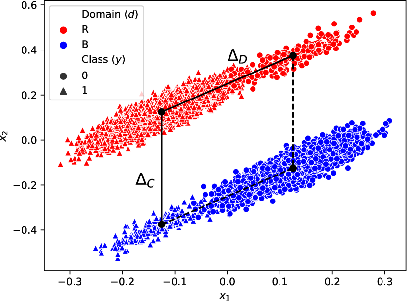
Figure 1: Sample drawn from a distribution satisfying Assumptions 3.3, 3.2, 3.4 and 3.5. $\Delta_{C}$ and $\Delta_{D}$ are shown as line segments between means.

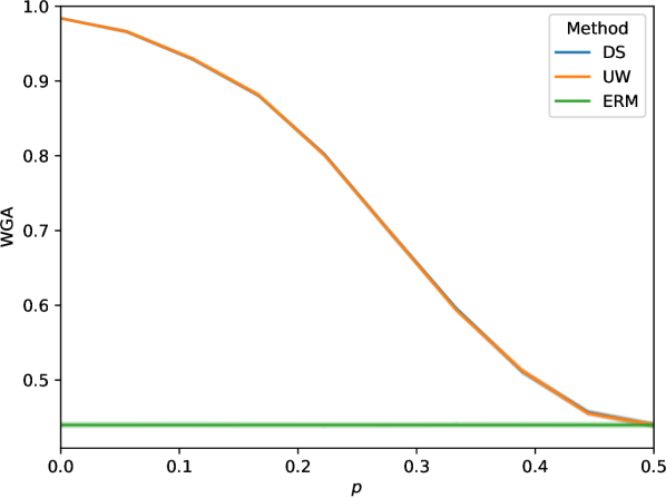
Figure 2: For data from the model given by (8), the WGA of DS and UW (seen as overlapping) decreases as the noise prevalence $p$ increases to $1/2$. At the extreme point, the WGA of ERM is recovered.

Assumption 3.2.

$X\in\mathcal{X}$ is distributed according to the following mixture of Gaussians:

$$X|(Y=y,D=d) \sim\mathcal{N}(\mu^{(y,d)},\Sigma),$$ (8)

for $(y,d)\in\mathcal{Y}\times\mathcal{D}$, where $\mu^{(y,d)}\coloneqq\mathbb{E}[X|Y=y,D=d]\in\mathbb{R}^{m}$ and $\Sigma\in\mathbb{R}^{m\times m}$ is a symmetric positive definite matrix. Additionally, we place priors $\pi^{(y,d)}$, $(y,d)\in\mathcal{Y}\times\mathcal{D}$, on each group and priors $\pi^{(y)}\coloneqq P(Y=y)$, $y\in\mathcal{Y}$, on each class.

Assumption 3.3.

The minority groups have equal priors, i.e., for $\pi_{0}\leq 1/4$,

$$\pi^{(0,R)}=\pi^{(1,B)}=\pi_{0}\text{ and }\pi^{(1,R)}=\pi^{(0,B)}=1/2-\pi_{0}.$$

Also, the class priors are equal, i.e., $\pi^{(0)}=\pi^{(1)}=1/2$.

Assumption 3.4.

The difference in means between classes in a domain $\Delta_{D}\coloneqq\mu^{(1,d)}-\mu^{(0,d)}$ is constant for $d\in\mathcal{D}$.

Assumption 3.4 also implies that the difference in means between domains within the same class $\Delta_{C}\coloneqq\mu^{(y,B)}-\mu^{(y,R)}$ is also constant for each $y\in\mathcal{Y}$. We see this by noting that each group mean makes up the vertex of a parallelogram. This is illustrated in Figure 2, where $\Delta_{D}$ and $\Delta_{C}$ are shown on data samples drawn from a distribution satisfying Assumptions 3.3, 3.2 and 3.4.

Assumption 3.5.

$\Delta_{D}$ and $\Delta_{C}$ are orthogonal with respect to $\Sigma^{-1}$, i.e., $\Delta_{C}^{T}\Sigma^{-1}\Delta_{D}=0$.

We see an example of a dataset drawn from a distribution satisfying Assumptions 3.3, 3.2, 3.4 and 3.5 in Figure 2. The data is generated with parameters,

$$\Delta_{C} =\begin{pmatrix}0&-0.5\end{pmatrix}^{T} \quad\Delta_{D} =\begin{pmatrix}-0.25&-0.25\end{pmatrix}^{T}$$

$$\Sigma =\begin{pmatrix}.003&.003\\ .003&.004\\ \end{pmatrix} \quad\pi_{0} =\frac{1}{50}.$$

While this is a simplified view of binary class, binary domain latent groups, these tractable assumptions allow us to make theoretical guarantees about the performance of downsampling and upweighting under noise. We see that the general trends observed in this simplified setting hold in large publicly available datasets in Section 5.3.

We now show that upweighting and downsampling achieve identical worst-group accuracy in the population setting (i.e., infinite samples) and both degrade with SLN in the domain annotation while ERM is unaffected by domain noise.

Theorem 3.6.

Consider the model of latent Gaussian groups satisfying Assumptions 3.3, 3.2, 3.4 and 3.5 with symmetric domain label noise with parameter $p$. Let $f_{\theta}(x)=w^{T}x+b$ and $\hat{Y}=\mathbbm{1}\{f_{\theta}(x)>1/2\}$. In this setting, let $\theta^{(p)}_{\text{UW}}$ and $\theta^{(p)}_{\text{DS}}$ denote the solution to (3) under squared loss for UW and DS, respectively. For any $\pi_{0}\in(0,1/4]$, the WGA of both augmentation approaches are equal and degrade smoothly in $p\in[0,1/2]$ to the baseline WGA of (3) with no augmentation (with optimal parameter $\theta_{\text{ERM}}$). That is,

$$WGA(\theta_{\text{ERM}})\leq WGA(\theta^{(p)}_{\text{DS}})=WGA(\theta^{(p)}_{\text{UW}})$$

with equality at $p=1/2$ or $\pi_{0}=1/4$ .

Proof Sketch.

The proof of Theorem 3.6 is presented in Appendix A and involves showing that the WGA for downsampling under domain label noise is the same as that for ERM (which is noise agnostic) but with a different prior dependent on $p$. Our proof refines the analysis in Yao et al. (2022) and involves the noisy prior.

Fundamentally, this result can be seen as an effect of the domain noise on the perceived (noisy) priors ${\pi}_{0}^{(p)}$ of the minority groups, which can be derived as

$$\pi_{0}^{(p)} \coloneqq(1-p)\pi_{0}+p\left(1/2-\pi_{0}\right).$$ (9)

As $p\rightarrow 1/2$ in (9), the minority prior perceived by both UW and DS tends to a balanced prior across groups. A UW augmentation thus would weight in inverse proportion to the corresponding noisy (and not the true) prior for each group. The true prior of the minority group after DS can be derived as (see Appendix A)

$$\pi_{\text{DS}}^{(p)}\coloneqq\frac{(1-p)\pi_{0}}{4\pi^{(p)}_{0}}+\frac{p\pi_{0}}{4(1/2-\pi^{(p)}_{0})}.$$ (10)

Thus, with noisy domain labels, instead of the desired balanced group priors after downsampling, from (10), DS results in a true minority prior that decreases from $1/4$ to $\pi_{0}$. Thus, noise in domain labels drives inaction from both augmented methods as $p$ increases.

We see the effect of noise in a numerical example in Figure 2, noting that while the theorem is in the statistical setting, our numerical example uses finite sample methods with $n=10,000$. This shows that the performance of each method quickly degrades even in this simple setting. The ERM performance, however, remains constant because ERM does not use domain information. This motivates us to examine a robust method which does not use domain information at all but is more effective than ERM in terms of WGA.

4 Regularized Annotation of Domains

When domain annotations are unavailable (or noisy), LaBonte et al. (2023) use implicitly regularized models trained on the imbalanced retraining data to annotate the data. We take a similar approach but explicitly regularize our pseudo-annotation model with an $\ell_{1}$ penalty. The intuition behind using an $\ell_{1}$ penalty is similar to that of DFR (Kirichenko et al., 2023). Where Kirichenko et al. (2023) argue that an $\ell_{1}$ penalty helps to select only “core features” when trained on a group-balanced dataset, we argue that the same penalty with a large multiplicative factor will help to select spuriously correlated features when trained on the original imbalanced data. If we can successfully learn the spuriously correlated features, those samples which are correctly classified can be viewed as majority samples (those for which the spurious correlation holds) and those which are misclassified can be seen as minority samples.

Algorithm 1 Regularized Annotation of Domains (RAD)

  Input: data $D=(x,y)$, annotator regularization $\lambda_{\text{ID}}$

  Train classifier $f_{\text{ID}}$ on $D$ with $\ell_{1}$ factor $\lambda_{\text{ID}}$

  for $(x_{i},y_{i})\in D$ do

     if $f_{\text{ID}}(x_{i})\neq y_{i}$ then

        $\tilde{d}_{i}\leftarrow 1$

     else

        $\tilde{d}_{i}\leftarrow 0$

     end if

  end for

  Return: $(x,y,\tilde{d})$, the pseudo-annotated data

We introduce RAD (Regularized Annotation of Domains) which uses a highly $\ell_{1}$ regularized linear model to pseudo-annotate domain information by quantizing true domains to binary majority and minority annotations. Pseudocode for this algorithm is presented in Algorithm 1.

RAD-UW involves learning sequentially: (i) a pseudo-annotation RAD model, and (ii) a regularized linear retraining model, which is trained on all examples while upweighting the pseudo-annotated minority examples output by RAD, as the solution $\hat{\theta}_{\text{RAD-UW}}^{*}$ optimizing the empirical version of (3) using the logistic loss $\ell_{L}$ with $\ell_{1}$ regularization as:

$$\hat{\theta}_{\text{RAD-UW}}^{*}=\operatorname*{arg\,min}_{\theta}\frac{1}{n}\sum_{i=1}^{n}c(y_{i},\tilde{d}_{i})\ell_{L}(f_{\theta}(x_{i}),y_{i})+\lambda\|w\|_{1}.$$ (11)

5 Empirical Results

We present worst-group accuracies for several representative methods across four large publicly available datasets. Note that for all datasets, we use the training split to train the embedding model. Following prior work (Kirichenko et al., 2023; LaBonte et al., 2023), we use half of the validation as retraining data and half as a clean holdout.

5.1 Datasets

CMNIST (Arjovsky et al., 2019) is a variant of the MNIST handwritten digit dataset in which digits 0-4 are labeled $y=0$ and digits 5-9 are labeled $y=1$. Further, 90% of digits labeled $y=0$ are colored green and 10% are colored red. The reverse is true for those labeled $y=1$. Thus, we can view color as a domain and we see that the color of the digit and its label are correlated.

CelebA (Liu et al., 2015) is a dataset of celebrity faces. For this data, we predict hair color as either blonde ($y=1$) or non-blonde ($y=0$) and use gender, either male ($d=1$) or female ($d=0$), as the domain label. There is a natural correlation in the dataset between hair color and gender because of the prevalence of blonde female celebrities.

Waterbirds (Sagawa et al., 2020) is a semi-synthetic dataset which places images of land birds ($y=1$) or sea birds ($y=0$) on land ($d=1$) or sea ($d=0$) backgrounds. There is a correlation between background and the type of bird in the training data but this correlation is removed in the validation data.

MultiNLI (Williams et al., 2018) is a text corpus dataset widely used in natural language inference tasks. For our setup, we use MultiNLI as first introduced in (Oren et al., 2019). Given two sentences, a premise and a hypothesis, our task is to predict whether the hypothesis is either entailed by, contradicted by, or neutral with the premise. There is a spurious correlation between there being a contradiction between the hypothesis and the premise and the presence of a negation word (no, never, etc.) in the hypothesis.

5.2 Experimental Details

Table 1: CMNIST WGA under domain label noise. CMNIST has a relatively small spurious correlation and as such even LLR performs quite well. Additionally, CMNIST is already class balanced so class downsampling and upweighting have no effect. (LaBonte et al., 2023) do not provide WGA for CMNIST; RAD-UW matches the performance of group-dependent methods at 10% and surpasses it beyond that.

Method	DA	Group Annotation Noise (%)
		0	5	10	15	20
Group Downsample	Y	$\mathbf{95.59\pm 0.42}$	$\mathbf{94.87\pm 0.41}$	$\mathbf{94.31\pm 0.48}$	$93.92\pm 0.48$	$93.28\pm 0.53$
Group Upweight	Y	$94.99\pm 0.25$	$94.32\pm 0.82$	$93.68\pm 0.85$	$93.34\pm 0.47$	$92.74\pm 0.42$
Class Downsample	N	$91.49\pm 0.72$	$91.78\pm 0.31$	$91.78\pm 0.31$	$91.78\pm 0.31$	$91.78\pm 0.31$
Class Upweight	N	$91.26\pm 0.86$	$91.47\pm 0.69$	$91.47\pm 0.69$	$91.47\pm 0.69$	$91.47\pm 0.69$
LLR	N	$91.44\pm 0.75$	$91.59\pm 0.30$	$91.59\pm 0.30$	$91.59\pm 0.30$	$91.59\pm 0.30$
RAD-UW	N	$94.29\pm 0.72$	$94.27\pm 0.75$	$94.27\pm 0.75$	$\mathbf{94.27\pm 0.75}$	$\mathbf{94.27\pm 0.75}$

Table 2: CelebA WGA under domain label noise. RAD-UW outperforms domain annotation-dependent methods at only 5% noise and existing misclassification-based domain annotation-free baselines at every noise level.

Method	DA	Group Annotation Noise (%)
		0	5	10	15	20
Group Downsample	Y	$\mathbf{86.00\pm 1.99}$	$82.40\pm 2.60$	$79.04\pm 3.37$	$78.59\pm 3.94$	$76.39\pm 3.46$
Group Upweight	Y	$85.17\pm 1.36$	$83.13\pm 1.90$	$81.61\pm 2.21$	$81.31\pm 0.70$	$78.56\pm 1.10$
Class Downsample	N	$73.97\pm 2.67$	$74.63\pm 1.55$	$74.63\pm 1.55$	$74.63\pm 1.55$	$74.63\pm 1.55$
Class Upweight	N	$73.89\pm 0.00$	$73.89\pm 0.00$	$73.89\pm 0.00$	$73.89\pm 0.00$	$73.89\pm 0.00$
LLR	N	$44.83\pm 1.24$	$44.95\pm 1.12$	$44.95\pm 1.12$	$44.95\pm 1.12$	$44.95\pm 1.12$
RAD-UW	N	$83.67\pm 0.54$	$\mathbf{83.67\pm 0.57}$	$\mathbf{83.67\pm 0.57}$	$\mathbf{83.67\pm 0.57}$	$\mathbf{83.67\pm 0.57}$
ESM-SELF	N	$80.4\pm 3.9$	$80.4\pm 3.9$	$80.4\pm 3.9$	$80.4\pm 3.9$	$80.4\pm 3.9$
M-SELF	N	$83.0\pm 6.1$	$83.0\pm 6.1$	$83.0\pm 6.1$	$83.0\pm 6.1$	$83.0\pm 6.1$

Table 3: Waterbirds WGA under domain label noise. The validation (retraining) split for Waterbirds is domain balanced already, so class and group balancing perform equivalently. All domain annotation-free methods show improvement over baselines.

Method	DA	Group Annotation Noise (%)
		0	5	10	15	20
Group Downsample	Y	$91.69\pm 0.88$	$91.76\pm 0.94$	$91.69\pm 0.79$	$91.49\pm 1.03$	$91.28\pm 1.00$
Group Upweight	Y	$91.30\pm 0.52$	$91.25\pm 0.47$	$91.28\pm 0.47$	$91.26\pm 0.48$	$91.29\pm 0.47$
Class Downsample	N	$91.83\pm 0.88$	$91.84\pm 0.63$	$91.84\pm 0.63$	$91.84\pm 0.63$	$91.84\pm 0.63$
Class Upweight	N	$91.31\pm 0.52$	$91.30\pm 0.52$	$91.30\pm 0.52$	$91.30\pm 0.52$	$91.30\pm 0.52$
LLR	N	$87.05\pm 1.25$	$87.06\pm 1.22$	$87.06\pm 1.22$	$87.06\pm 1.22$	$87.06\pm 1.22$
RAD-UW	N	$\mathbf{92.62\pm 0.26}$	$\mathbf{92.62\pm 0.26}$	$\mathbf{92.62\pm 0.26}$	$\mathbf{92.62\pm 0.26}$	$\mathbf{92.62\pm 0.26}$
ESM-SELF	N	$92.2\pm 0.7$	$92.2\pm 0.7$	$92.2\pm 0.7$	$92.2\pm 0.7$	$92.2\pm 0.7$
M-SELF	N	$92.6\pm 0.8$	$92.6\pm 0.8$	$92.6\pm 0.8$	$92.6\pm 0.8$	$92.6\pm 0.8$

Table 4: MultiNLI WGA under domain label noise. SELF performs strongly on this dataset, perhaps due to the structure of the spurious correlation. Regardless, both SELF and RAD-UW outperform group-dependent methods at label noise above 5%.

Method	DA	Group Annotation Noise (%)
		0	5	10	15	20
Group Downsample	Y	$73.10\pm 1.01$	$68.11\pm 1.07$	$65.48\pm 0.83$	$65.16\pm 0.59$	$65.44\pm 0.42$
Group Upweight	Y	$\mathbf{74.18\pm 0.39}$	$68.19\pm 0.68$	$66.01\pm 0.27$	$65.32\pm 0.49$	$65.59\pm 0.48$
Class Downsample	N	$65.22\pm 0.42$	$65.51\pm 0.19$	$65.51\pm 0.19$	$65.51\pm 0.19$	$65.51\pm 0.19$
Class Upweight	N	$65.35\pm 0.36$	$65.42\pm 0.35$	$65.42\pm 0.35$	$65.42\pm 0.35$	$65.42\pm 0.35$
LLR	N	$65.36\pm 0.35$	$65.47\pm 0.31$	$65.47\pm 0.31$	$65.47\pm 0.31$	$65.47\pm 0.31$
RAD-UW	N	$68.10\pm 0.98$	$68.10\pm 0.98$	$68.10\pm 0.98$	$68.10\pm 0.98$	$68.10\pm 0.98$
ESM-SELF	N	$73.3\pm 1.2$	$\mathbf{73.3\pm 1.2}$	$\mathbf{73.3\pm 1.2}$	$\mathbf{73.3\pm 1.2}$	$\mathbf{73.3\pm 1.2}$
M-SELF	N	$72.2\pm 2.2$	$72.2\pm 2.2$	$72.2\pm 2.2$	$72.2\pm 2.2$	$72.2\pm 2.2$

We present results for both group- and class-only-dependent methods using both downsampling and upweighting. Additionally, we present results for vanilla LLR, which performs no data or loss augmentation step before retraining. Finally, we present results for RAD with upweighting, i.e., RAD-UW. Every retraining method solves the following empirical optimization problem:

$$\hat{\theta}^{*}=\operatorname*{arg\,min}_{\theta}\frac{1}{n}\sum_{i=1}^{n}c(d_{i},y_{i})\ell(f_{\theta}(x_{i}),y_{i})+\lambda\|w\|_{1},$$ (12)

which can be seen as a finite sample version of (3) with an $\ell_{1}$ regularization. In practice, we use the logistic loss.

Methods which require domain annotations (DA) are denoted with a “Y” in the appropriate column, while those which are agnostic to DA are denoted as “N”. We collate the results of similar methods and separate those for different approaches in our tables by horizontal lines. Finally, results for methods designed to annotate domains before using data augmentations including RAD-UW and SELF (LaBonte et al., 2023) are collected at the bottom of each table.

The group-dependent downsampling procedure we have adopted is the same as that of DFR, introduced in Kirichenko et al. (2023), but the DFR methodology averages the learned model over 10 training runs. This could help to reduce the variance, but we do not implement this so as to directly compare different data augmentation methods since most others do not so either. More generally, we could apply model averaging to any of the data augmentation methods.

We use the logistic regression implementation from the scikit-learn (Pedregosa et al., 2011) package for the retraining step for all presented methods. For all final retraining steps (including LLR) an $\ell_{1}$ regularization is added. The strength of the regularization $\lambda$ is a hyperparameter selected using the clean holdout. The upweighting factor for group annotation-inclusive UW methods is given by the inverse of the perceived prevalence for each group or class.

For our RAD-UW method, we tune the regularization strength $\lambda_{\text{ID}}$ for the pseudo-annotation model. We additionally tune the regularization strength $\lambda$ of the retraining model along with the upweighting factor $c$, which is left as a hyperparameter because the identification of domains by RAD is only binary and may not reflect the domains in the clean holdout data. The same upweighting factor is used for every pseudo-annotated minority sample.

Note that for all of the WGA results, we report the mean WGA over 10 independent noise seeds and 10 training runs for each noise seed. We also present the standard deviation around this mean, which will reflect the variance over training runs with the optimal hyperparameters. For ES misclassification SELF (ESM-SELF) and misclassification SELF (M-SELF) (LaBonte et al., 2023), we present their results directly. It should be noted that they report the mean and standard deviation over only three independent runs and without noise; for the noisy setting, we assume their results remain unchanged with domain noise.

5.3 Worst-Group Accuracy under Noise

We now detail the results on all datasets in Tables 2, 1, 4 and 3. See Appendix D for a visual representation of these results.

For CMNIST, we present results in Table 1; we see that each method that uses domain information achieves strong WGA at 0% domain annotation noise, but for increasing noise, their performance drops noticeably. Additionally the methods which rely only on class labels without inferring domain membership are consistent across noise levels, but are outdone by their domain-dependent counterparts even at 20% noise. Finally, RAD-UW achieves WGA comparable with the group-dependent methods, and surpasses their performance after 10% noise in domain annotation.

The results for CelebA are presented in Table 2. We first note that LLR achieves significantly lower WGA than any other method owing to strong spurious correlation even in the retraining data. We also note that every domain-dependent method has a much more significant decline in performance for CelebA than for CMNIST. Here, RAD-UW outperforms the domain-dependent methods even at 5% SLN. Not only this, but RAD beats the performance of SELF (LaBonte et al., 2023) for this dataset with much lower variance.

For Waterbirds, we see in Table 3 that noise, even significant amounts of it, has little effect on any of the methods considered. This is because the existing splits have a domain-balanced validation, which we use here for retraining. Thus domain noise does not affect the group priors at all as argued analytically in (9) with $\pi_{0}=1/4$. Even so, we see that RAD-UW outperforms existing methods, including the domain annotation-free methods of LaBonte et al. (2023).

Finally, for MultiNLI, we see in Table 4 that RAD-UW is able to match domain-dependent methods at 5% noise and outperform them at 10%, but is beaten by the domain annotation-free methods of LaBonte et al. (2023). This may be because MultiNLI has weaker spurious correlation than the other datasets we examine. Also important to note is the effect of noise on MultiNLI. For 5% and 10% noise levels, we see a dramatic drop in WGA for domain-dependent methods, but this levels off as we recover the WGA of LLR. Thus even for 10% noise, LLR is competitive with top domain-dependent methods.

An interesting observation is that for almost all datasets and noise levels, the variance of group-dependent downsampling is consistently larger than upweighting at the same noise levels. This behavior is likely caused by two key issues: (i) DS reduces the dataset size, and (ii) it randomly subsamples the majority, each of which could increase the variance of the resulting classifier. DFR (Kirichenko et al., 2023) has attempted to remedy this issue by averaging the linear model that is learned over 10 different random downsamplings, but this increases the complexity of learning the final model. Our results raise questions on the prevalence of downsampling over the highly competitive upweighting method in the setting of WGA.

Finally, we consider the opportunity cost of ignoring domain annotations in the worst case, i.e., the domain labels we have are in fact noise-free but we still ignore them. In Figure 3, we see that the domain annotation-free methods cost very little in terms of lost WGA when training on cleanly annotated data. This loss is minimal in comparison to the cost of training using an annotation-dependent method when the domain information is noisy. Thus, if there are concerns about domain annotation noise in the training data, it is safest to use a domain annotation-free approach.

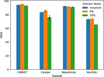
Figure 3: The cost of ignoring domain annotations. For each of the datasets, we compare the WGA of the best domain-dependent method at 0% and 20% domain noise with the best WGA amongst the methods which do not use domain information (labeled “Invariant”). The cost of ignoring the domain information is very small for most datasets and in Waterbirds, utilizing domain information hurts performance somewhat. Thus, the opportunity cost of not using domain information is relatively small, while the cost of using a domain-dependent method with noise is quite large.

6 Discussion

We see in our experiments that these two archetypal data augmentation techniques, downsampling and upweighting, achieve very similar worst-group accuracy and degrade similarly with noise. This falls in line with our theoretical analysis, and suggests that simple Gaussian mixture models for subpopulations can provide intuition for the performance of data-augmented last layer retraining methods on real datasets.

Our experiments also indicate that downsampling induces a higher variance in WGA, especially in the noisy domain annotation setting. While this phenomenon is not captured in our statistical analysis, intuitively one should expect that having a smaller dataset should increase the variance. Additionally, the models learned by group downsampling suffer from an additional dependence on the data that is selected in downsampling, which in turn increases the WGA variance.

Overall, we demonstrate that achieving SOTA worst-group accuracy is strongly dependent on the quality of the domain annotations on large publicly available datasets. Our experiments consistently show that in order to be robust to noise in the domain annotations, it is necessary to ignore them altogether. To this end, our novel domain annotation-free method, RAD-UW, assures WGA values competitive with annotation-inclusive methods. RAD-UW does so by pseudo-annotating with a highly regularized model that allows discriminating between samples with spurious features and those without and retraining on the latter with upweighting. Our comparison of RAD-UW to two existing domain annotation-free methods and several domain annotation-dependent methods clearly highlights that it can outperform existing methods even for only 5% domain label noise.

There is a significant breadth of future work available in this area. In the domain annotation-free setting, there is a gap in the literature regarding identification of subpopulations beyond the binary “minority,” or “majority” groups. Identifying individual groups could help to increase the performance of retrained models and give better insight into which groups are negatively affected by vanilla LLR. Additionally, tuning hyperparameters without a clean holdout set remains an open question.

Beyond this, group noise could be driven by class label noise alongside domain annotation noise. The combination of these two types of noise would necessitate a robust loss function when training both the pseudo-annotation and retraining models, or a new approach entirely. We are optimistic that the approach presented here could be combined in a modular fashion with a robust loss to achieve robustness to more general group noise.

Appendix A Proof of Theorem 3.6

Our proof can be outlined as involving five steps; these steps rely on Proposition 3.1 and include three new lemmas. We enumerate the steps below:

1. We first show in Lemma A.1 that ERM is agnostic to domain label noise.

2. We next show in Lemma A.2 that for clean data with any minority prior $\pi_{0}$, the WGA for ERM is given by (13)

3. In Equation 37 we show that the model learned after downsampling with noisy domain labels is equivalent to a clean ERM model learned with prior

   $$\frac{(1-p)\pi_{0}}{4\pi_{0}^{(p)}}+\frac{p\pi_{0}}{4\big{(}1/2-\pi_{0}^{(p)}\big{)}}.$$

4. We then show that the WGA of downsampling strictly decreases in $p$ by examining the derivative.

5. Finally we note that by Proposition 3.1, upweighting must learn the same model as downsampling

We present the three lemmas below and use them to complete the proof.

Lemma A.1.

ERM with no data augmentation is agnostic to the domain label noise $p$, i.e., the model learned by ERM in (3) in the setting of domain label noise is the same as that learned in the setting of clean domain labels (no noise).

Proof.

Since ERM with no data augmentation does not use domain label information when learning a model, the model will remain unchanged under domain label noise. ∎

Lemma A.2.

Let $\theta_{\text{ERM}}$ denote the optimal model parameter learned by ERM in (3) using $f_{\theta}(x)=w^{T}x+b$ and $\hat{Y}=\mathbbm{1}\{f_{\theta}(x)>1/2\}$. Under Assumptions 3.3, 3.2, 3.4 and 3.5,

$$\text{WGA}({\theta_{\text{ERM}}})=\Phi\left(\frac{\|\Delta_{D}\|^{2}-\tilde{c}_{\pi_{0}}\|\Delta_{C}\|^{2}}{2(\|\Delta_{D}\|+\tilde{c}_{\pi_{0}}\|\Delta_{C}\|)}\right),$$ (13)

where $\tilde{c}_{\pi_{0}}\coloneqq({1-4\pi_{0}})/({1+2\pi_{0}(1-2\pi_{0})\|\Delta_{C}\|^{2}})$ and $\|v\|\coloneqq\sqrt{v^{T}\Sigma^{-1}v}$.

Proof.

Since the model learned by ERM with no data augmentation is invariant to domain label noise by Lemma A.1, we derive the the general form for the WGA of a model $f_{\theta}$ under the assumption of having clean domain label, and therefore using the original data parameters. We begin by deriving the individual accuracy terms $A^{(y,d)}(f_{\theta})$, $(y,d)\in\{0,1\}\times\{R,B\}$, with $f_{\theta}(x)=w^{T}x+b$ and $\hat{Y}=\mathbbm{1}\{f_{\theta}(x)>1/2\}$, as follows:

$$A^{(1,d)}(f_{\theta}) \coloneqq P\left(\mathbbm{1}\left\{w^{T}X+b>1/2\right\}=Y\mid Y=1,D=d\right)$$

$$=P\left(w^{T}X+b>1/2\mid Y=1,D=d\right)$$

$$=1-\Phi\left(\frac{1/2-(w^{T}\mu^{(1,d)}+b)}{\sqrt{w^{T}\Sigma w}}\right)$$

$$=\Phi\left(\frac{w^{T}\mu^{(1,d)}+b-1/2}{\sqrt{w^{T}\Sigma w}}\right),$$

$$A^{(0,d)}(f_{\theta}) \coloneqq P\left(\mathbbm{1}\left\{w^{T}X+b>1/2\right\}=Y\mid Y=0,D=d\right)$$

$$=P\left(w^{T}X+b\leq 1/2\mid Y=0,D=d\right)$$

$$=\Phi\left(\frac{1/2-(w^{T}\mu^{(0,d)}+b)}{\sqrt{w^{T}\Sigma w}}\right).$$

We now derive the optimal model parameters for ERM for any $\pi_{0}\leq 1/4$. In the case of ERM, $c(y,d)=1$ for $(y,d)\in\mathcal{Y}\times\mathcal{D}$, so the optimal solution to (3) with $f_{\theta}(x)=w^{T}x+b$ and $\hat{Y}=\mathbbm{1}\{f_{\theta}(x)>1/2\}$ is

$$w_{\text{ERM}}=\text{Var}(X)^{-1}\text{Cov}(X,Y),\quad\text{and}\quad b_{\text{ERM}}=\mathbb{E}[Y]-w^{T}\mathbb{E}[X].$$ (14)

Note that

$$\mathbb{E}[Y] =\frac{1}{2},$$

$$\mathbb{E}[X] =\mathbb{E}\left[\mathbb{E}[X|D,Y]\right]$$

$$=\sum_{(y,d)\in\{0,1\}\times\{R,B\}}[\mathbbm{1}(d=R)(\mu^{(0,R)}-\mu^{(0,B)})+(1-y)\mu^{(0,B)}+y\mu^{(1,B)}]\pi^{(y,d)}$$

$$=\frac{1}{2}(\mu^{(0,R)}+\mu^{(1,B)}).$$

Let $\pi^{(d|y)}\coloneqq P(D=d|Y=y)$ for $(y,d)\in\mathcal{Y}\times\mathcal{D}$, $\mu^{(y)}\coloneqq\mathbb{E}[X|Y=y]$ for $y\in\mathcal{Y}$ and $\bar{\Delta}\coloneqq\mu^{(1)}-\mu^{(0)}$. We compute $\text{Var}(X)$ as follows:

$$\text{Var}(X) =\mathbb{E}[\text{Var}(X|Y)]+\text{Var}(\mathbb{E}[X|Y])$$ (15)

$$=\mathbb{E}\left[\mathbb{E}[\text{Var}(X|Y,D)|Y]+\text{Var}(\mathbb{E}[X|Y,D]|Y)\right]+\text{Var}(\mathbb{E}[X|Y])$$ (16)

$$=\Sigma+\mathbb{E}[\text{Var}(\mathbb{E}[X|Y,D]|Y)]+\text{Var}(\mathbb{E}[X|Y])$$ (17)

$$=\Sigma+\mathbb{E}[\text{Var}(\mathbbm{1}(D=R)(\mu^{(0,R)}-\mu^{(0,B)})+(1-Y)\mu^{(0,B)}+Y\mu^{(1,B)}|Y)]+\text{Var}(\mathbb{E}[X|Y])$$ (18)

$$=\Sigma+\Delta_{C}\Delta_{C}^{T}\mathbb{E}[\text{Var}(\mathbbm{1}(D=R)|Y)]+\text{Var}(Y(\mu^{(1)}-\mu^{(0)})+\mu^{(0)})$$ (19)

$$=\Sigma+\Delta_{C}\Delta_{C}^{T}\mathbb{E}[\text{Var}(D|Y)]+\bar{\Delta}\bar{\Delta}^{T}\text{Var}(Y)$$ (20)

$$=\Sigma+\Delta_{C}\Delta_{C}^{T}\mathbb{E}[Y\pi^{(R|1)}\pi^{(B|1)}+(1-Y)\pi^{(R|0)}\pi^{(B|0)}]+\bar{\Delta}\bar{\Delta}^{T}\pi^{(1)}\pi^{(0)}$$ (21)

$$=\Sigma+2\pi_{0}(1-2\pi_{0})\Delta_{C}\Delta_{C}^{T}+\frac{1}{4}\bar{\Delta}\bar{\Delta}^{T}.$$ (22)

Next, we compute $\text{Cov}(X,Y)$ as follows:

$$\text{Cov}(X,Y) =\mathbb{E}[\text{Cov}(X,Y|Y)]+\text{Cov}(\mathbb{E}[X|Y],\mathbb{E}[Y|Y])$$ (23)

$$=\text{Cov}(\mathbb{E}[X|Y],Y)$$ (24)

$$=\text{Cov}(\mu^{(0)}+Y\bar{\Delta},Y)$$ (25)

$$=\text{Cov}(Y\bar{\Delta},Y)$$ (26)

$$=\bar{\Delta}\text{Var}(Y)$$ (27)

$$=\pi^{(1)}\pi^{(0)}\bar{\Delta}$$ (28)

$$=\frac{1}{4}\bar{\Delta}.$$ (29)

In order to write (22) and (29) only in terms of $\Delta_{C}$ and $\Delta_{D}$ and to see the effect of $\pi_{0}$, we show the following relationship between $\bar{\Delta}$, $\Delta_{C}$ and $\Delta_{D}$.

We introduce the following two minor lemmas that allow us to obtain clean expression for the optimal weights.

Lemma A.3.

Let $\bar{\Delta}\coloneqq\mu^{(1)}-\mu^{(0)}$. Then

$$\Delta_{D}-\bar{\Delta}=(1-4\pi_{0})\Delta_{C}$$

Proof.

We first note that

$$\mu^{(1)}=2\pi_{0}(\mu^{(1,B)}-\mu^{(1,R)})+\mu^{(1,R)}=2\pi_{0}\Delta_{C}+\mu^{(1,R)}.$$

Similarly,

$$\mu^{(0)}=2\pi_{0}(\mu^{(0,R)}-\mu^{(0,B)})+\mu^{(0,B)}=-2\pi_{0}\Delta_{C}+\mu^{(0,B)}.$$

Combining these with the definitions of $\Delta_{D}$ and $\bar{\Delta}$, we get

$$\Delta_{D}-\bar{\Delta} =\Delta_{D}-(\mu^{(1)}-\mu^{(0)})$$

$$=\mu^{(1,R)}-\mu^{(0,R)}-2\pi_{0}\Delta_{C}-\mu^{(1,R)}-2\pi_{0}\Delta_{C}+\mu^{(0,B)}$$

$$=\mu^{(0,B)}-\mu^{(0,R)}-4\pi_{0}\Delta_{C}$$

$$=(1-4\pi_{0})\Delta_{C}.$$

∎

From (22), (29) and Lemma A.3, we then obtain

$$w_{\text{ERM}}=\frac{1}{4}\left(\Sigma+2\pi_{0}(1-2\pi_{0})\Delta_{C}\Delta_{C}^{T}+\frac{1}{4}\bar{\Delta}\bar{\Delta}^{T}\right)^{-1}\bar{\Delta},$$ (30)

where $\bar{\Delta}\coloneqq\mu^{(1)}-\mu^{(0)}=\Delta_{D}-(1-4\pi_{0})\Delta_{C}$, and

$$b_{\text{ERM}}=\frac{1}{2}-\frac{1}{2}(w_{\text{ERM}})^{T}(\mu^{(0,R)}+\mu^{(1,B)}).$$ (31)

Therefore,

$$A^{(1,d)}(f_{\theta_{\text{ERM}}}) =\Phi\left(\frac{(w_{\text{ERM}})^{T}\left(\mu^{(1,d)}-\frac{1}{2}(\mu^{(0,R)}-\mu^{(1,B)})\right)}{\sqrt{(w_{\text{ERM}})^{T}\Sigma w_{\text{ERM}}}}\right),$$ (32)

$$A^{(0,d)}(f_{\theta_{\text{ERM}}}) =\Phi\left(\frac{-(w_{\text{ERM}})^{T}\left(\mu^{(0,d)}-\frac{1}{2}(\mu^{(0,R)}-\mu^{(1,B)})\right)}{\sqrt{(w_{\text{ERM}})^{T}\Sigma w_{\text{ERM}}}}\right).$$ (33)

We can simplify the expressions in (32) and (33) by using the following relations:

$$\mu^{(0,R)}-\frac{1}{2}(\mu^{(0,R)}-\mu^{(1,B)}) =\frac{1}{2}(\mu^{(0,R)}-\mu^{(1,B)})=\frac{1}{2}(\mu^{(0,R)}-\mu^{(1,R)}+\mu^{(1,R)}-\mu^{(1,B)})=-\frac{1}{2}(\Delta_{C}+\Delta_{D}),$$

$$\mu^{(0,B)}-\frac{1}{2}(\mu^{(0,R)}-\mu^{(1,B)}) =\frac{1}{2}(\mu^{(0,B)}-\mu^{(0,R)})+\frac{1}{2}(\mu^{(0,B)}-\mu^{(1,B)})=\frac{1}{2}(\Delta_{C}-\Delta_{D}),$$

$$\mu^{(1,B)}-\frac{1}{2}(\mu^{(0,R)}-\mu^{(1,B)}) =\frac{1}{2}(\mu^{(1,B)}-\mu^{(0,R)})=\frac{1}{2}(\mu^{(1,B)}-\mu^{(1,R)}+\mu^{(1,R)}-\mu^{(0,R)})=\frac{1}{2}(\Delta_{C}+\Delta_{D}),$$

$$\mu^{(1,R)}-\frac{1}{2}(\mu^{(0,R)}-\mu^{(1,B)}) =\frac{1}{2}(\mu^{(1,R)}-\mu^{(0,R)})+\frac{1}{2}(\mu^{(1,R)}-\mu^{(1,B)})=\frac{1}{2}(\Delta_{D}-\Delta_{C}).$$

Plugging these into (32) and (33) for each group $(y,d)\in\{0,1\}\times\{R,B\}$ yields

$$A^{(0,R)}(f_{\theta_{\text{ERM}}}) =A^{(1,B)}(f_{\theta_{\text{ERM}}})=\Phi\left(\frac{\frac{1}{2}(w_{\text{ERM}})^{T}\left(\Delta_{C}+\Delta_{D}\right)}{\sqrt{(w_{\text{ERM}})^{T}\Sigma w_{\text{ERM}}}}\right),$$

$$A^{(0,B)}(f_{\theta_{\text{ERM}}}) =A^{(1,R)}(f_{\theta_{\text{ERM}}})=\Phi\left(\frac{\frac{1}{2}(w_{\text{ERM}})^{T}\left(\Delta_{D}-\Delta_{C}\right)}{\sqrt{(w_{\text{ERM}})^{T}\Sigma w_{\text{ERM}}}}\right).$$

Thus,

$$\text{WGA}(\theta_{\text{ERM}})=\min\left\{\Phi\left(\frac{\frac{1}{2}(w_{\text{ERM}})^{T}\left(\Delta_{C}+\Delta_{D}\right)}{\sqrt{(w_{\text{ERM}})^{T}\Sigma w_{\text{ERM}}}}\right),\Phi\left(\frac{\frac{1}{2}(w_{\text{ERM}})^{T}\left(\Delta_{D}-\Delta_{C}\right)}{\sqrt{(w_{\text{ERM}})^{T}\Sigma w_{\text{ERM}}}}\right)\right\}$$ (34)

In order to rewrite (30) to be able to simplify (34), we will use the following lemma.

Lemma A.4.

Let $A\in\mathbb{R}^{m\times m}$ be symmetric positive definite (SPD) and $u,v\in\mathbb{R}^{m}$. Then

$$(A+vv^{T}+uu^{T})^{-1}u=c_{u}\left(A^{-1}u-c_{v}A^{-1}v\right)\quad\text{with}\quad c_{u}\coloneqq\frac{1}{1+u^{T}B^{-1}u}\quad\text{and}\quad c_{v}\coloneqq\frac{v^{T}A^{-1}u}{1+v^{T}A^{-1}v}.$$

Proof.

Let $B\coloneqq A+vv^{T}$. Then

$$(A+vv^{T}+uu^{T})^{-1}u =(B+uu^{T})^{-1}u$$

$$=\left(B^{-1}-\frac{B^{-1}uu^{T}B^{-1}}{1+u^{T}B^{-1}u}\right)u\qquad\text{(Sherman-Morrison formula)}$$

$$=B^{-1}u-\frac{u^{T}B^{-1}u}{1+u^{T}B^{-1}u}B^{-1}u$$

$$=c_{u}B^{-1}u$$

$$=c_{u}\left(A^{-1}-\frac{A^{-1}vv^{T}A^{-1}}{1+v^{T}A^{-1}v}\right)u\qquad\text{(Sherman-Morrison formula)}.$$

The assumption that $A$ is SPD guarantees that $A^{-1}$ exists, $B$ is SPD, and $c_{u}$ and $c_{v}$ are well-defined. ∎

Applying Lemma A.4 to (30) with $A=\Sigma$, $u=\bar{\Delta}/2$ and $v=\sqrt{\beta}\Delta_{C}$, where $\beta\coloneqq 2\pi_{0}(1-2\pi_{0})$, yields

$$w_{\text{ERM}} =\gamma_{\text{ERM}}\left(\Sigma^{-1}\bar{\Delta}-\frac{\beta\Delta_{C}^{T}\Sigma^{-1}\bar{\Delta}}{1+\beta\Delta_{C}^{T}\Sigma^{-1}\Delta_{C}}\Sigma^{-1}\Delta_{C}\right)$$

$$=\gamma_{\text{ERM}}\left(\Sigma^{-1}\Delta_{D}-\frac{\delta+\beta\Delta_{C}^{T}\Sigma^{-1}\Delta_{D}}{1+\beta\Delta_{C}^{T}\Sigma^{-1}\Delta_{C}}\Sigma^{-1}\Delta_{C}\right)\qquad\text{(substituting $\bar{\Delta}=\Delta_{D}-\delta\Delta_{C}$)}$$

$$=\gamma_{\text{ERM}}\left(\Sigma^{-1}\Delta_{D}-c_{\pi_{0}}\Sigma^{-1}\Delta_{C}\right)$$

with

$$\gamma_{\text{ERM}}\coloneqq\frac{1}{4+\bar{\Delta}^{T}A_{\text{ERM}}^{-1}\bar{\Delta}}\quad\text{and}\quad c_{\pi_{0}}\coloneqq\frac{\delta+\beta\Delta_{C}^{T}\Sigma^{-1}\Delta_{D}}{1+\beta\Delta_{C}^{T}\Sigma^{-1}\Delta_{C}}.$$

Let $\|v\|\coloneqq\sqrt{v^{T}\Sigma^{-1}v}$ be the norm induced by the $\Sigma^{-1}$–inner product. Then

$$\text{WGA}({\theta_{\text{ERM}}}) =\min\Bigg{\{}\Phi\left(\frac{(1-c_{\pi_{0}})\Delta_{C}^{T}\Sigma^{-1}\Delta_{D}+\|\Delta_{D}\|^{2}-c_{\pi_{0}}\|\Delta_{C}\|^{2}}{2\|{\Delta_{D}-c_{\pi_{0}}\Delta_{C}}\|}\right),$$

$$\qquad\qquad\qquad\Phi\left(\frac{-(c_{\pi_{0}}+1)\Delta_{C}^{T}\Sigma^{-1}\Delta_{D}+\|\Delta_{D}\|^{2}+c_{\pi_{0}}\|\Delta_{C}\|^{2}}{\|\Delta_{D}-c_{\pi_{0}}\Delta_{C}\|}\right)\Bigg{\}}$$

Under Assumption 3.5, $c_{\pi_{0}}=\tilde{c}_{\pi_{0}}\coloneqq({1-4\pi_{0}})/({1+2\pi_{0}(1-2\pi_{0})\|\Delta_{C}\|^{2}})$ and

$$\text{WGA}({\theta_{\text{ERM}}})=\min\left\{\Phi\left(\frac{\|\Delta_{D}\|^{2}-\tilde{c}_{\pi_{0}}\|\Delta_{C}\|^{2}}{2(\|{\Delta_{D}}\|+\tilde{c}_{\pi_{0}}\|{\Delta_{C}}\|)}\right),\Phi\left(\frac{\|\Delta_{D}\|^{2}+\tilde{c}_{\pi_{0}}\|\Delta_{C}\|^{2}}{2(\|{\Delta_{D}}\|+\tilde{c}_{\pi_{0}}\|{\Delta_{C}}\|)}\right)\right\},$$ (35)

where the first term is the accuracy of the minority groups and the second is that of the majority groups. In order to compare the WGA of ERM with the WGA of DS, we first show that under Assumption 3.5 the WGA of ERM is given by the majority accuracy term in (35). Since $\tilde{c}_{\pi_{0}}\geq 0$ for $\pi_{0}\leq 1/4$, we have that

$$\frac{\|\Delta_{D}\|^{2}-\tilde{c}_{\pi_{0}}\|\Delta_{C}\|^{2}}{2(\|\Delta_{D}\|+\tilde{c}_{\pi_{0}}\|\Delta_{C}\|)}\leq\frac{\|\Delta_{D}\|^{2}+\tilde{c}_{\pi_{0}}\|\Delta_{C}\|^{2}}{2(\|\Delta_{D}\|+\tilde{c}_{\pi_{0}}\|\Delta_{C}\|)}\quad\Leftrightarrow\quad\tilde{c}_{\pi_{0}}\|\Delta_{C}\|^{2}\geq 0,$$

which is satisfied for all $\pi_{0}\leq 1/4$ with equality at $\pi_{0}=1/4$. Since $\Phi$ is increasing, we get

$$\text{WGA}({\theta_{\text{ERM}}})=\Phi\left(\frac{\|\Delta_{D}\|^{2}-\tilde{c}_{\pi_{0}}\|\Delta_{C}\|^{2}}{2(\|\Delta_{D}\|+\tilde{c}_{\pi_{0}}\|\Delta_{C}\|)}\right).$$ (36)

∎

Lemma A.5.

Learning the model in (3) after downsampling according to noisy domain labels using the noisy minority prior $\pi^{(p)}_{0}\coloneqq(1-p)\pi_{0}+p(1/2-\pi_{0})$ for $p\in[0,1/2]$ is equivalent to learning the model with clean domain labels (no noise) and using the minority prior

$$\pi_{\text{DS}}^{(p)}\coloneqq\frac{(1-p)\pi_{0}}{4\pi^{(p)}_{0}}+\frac{p\pi_{0}}{4(1/2-\pi^{(p)}_{0})}.$$ (37)

Proof.

We note that the model learned after downsampling is agnostic to domain labels, so only the true proportion of each group, not the noisy proportion, determines the model weights. We derive the equivalent clean prior. We do so by examining how true minority samples are affected by DS on the data with noisy domain labels. When DS is performed on the data with domain label noise, the true minority samples that are kept can be categorized as (i) those that are still minority samples in the noisy data and (ii) a proportion of those that have become majority samples in the noisy data.

The first type of samples appear with probability

$$(1-p)\pi_{0},$$ (38)

i.e., the proportion of true minority samples whose domain was not flipped. The second type of samples are kept with probability

$$p\pi_{0}\left(\frac{\pi^{(p)}_{0}}{1/2-\pi^{(p)}_{0}}\right),$$ (39)

where the factor dependent on $\pi_{0}^{(p)}$ is the factor by which the size of the noisy majority groups will be reduced to be the same size as the noisy minority groups.

Therefore, the unnormalized true minority prior can be written as

$$(1-p)\pi_{0}+p\pi_{0}\left(\frac{\pi^{(p)}_{0}}{1/2-\pi^{(p)}_{0}}\right).$$ (40)

We can repeat the same analysis for the majority groups to obtain the unnormalized true majority prior as

$$p(1/2-\pi_{0})+(1-p)(1/2-\pi_{0})\left(\frac{\pi^{(p)}_{0}}{1/2-\pi^{(p)}_{0}}\right).$$ (41)

In order for the true minority and true majority priors to sum to one over the four groups, we divide by the normalization factor $4\pi_{0}^{(p)}$, so our final minority prior is given by

$$\frac{(1-p)\pi_{0}+p\pi_{0}\left(\frac{\pi^{(p)}_{0}}{1/2-\pi^{(p)}_{0}}\right)}{4\pi_{0}^{(p)}}=\frac{(1-p)\pi_{0}}{4\pi_{0}^{(p)}}+\frac{p\pi_{0}}{4(1/2-\pi_{0}^{(p)})}.$$ (42)

∎

DS is usually a special case of ERM with $\pi_{0}=1/4$. However, since DS uses domain labels and therefore is not agnostic to noise, we need to use the prior derived in Equation 37 to be able to analyze the effect of the noise $p$ while still using the clean data parameters. Note that $\pi_{\text{DS}}^{(p)}$ defined in (37) decreases from $1/4$ to $\pi_{0}$ as the noise $p$ increases from $0$ to $1/2$. Since we can interpolate between $1/4$ to $\pi_{0}$ using $p$, we can therefore substitute $\pi_{0}$ in (13) with $\pi_{\text{DS}}^{(p)}$ and then examine the resulting expression as a function of $p$ for any $\pi_{0}$. Using the WGA of ERM from Lemma A.2, we take the following derivative:

$$\frac{\partial}{\partial p}\frac{\|\Delta_{D}\|^{2}-\tilde{c}_{\pi_{\text{DS}}^{(p)}}\|\Delta_{C}\|^{2}}{2\left(\|\Delta_{D}\|+\tilde{c}_{\pi_{\text{DS}}^{(p)}}\|\Delta_{C}\|\right)} =\frac{-\|\Delta_{D}\|\|\Delta_{C}\|(\|\Delta_{D}\|+\|\Delta_{C}\|)}{2\left(\|\Delta_{D}\|+\tilde{c}_{\pi_{\text{DS}}^{(p)}}\|\Delta_{C}\|\right)^{2}}\times\frac{-2\left(16\left(\pi_{\text{DS}}^{(p)}\right)^{2}-8\pi_{\text{DS}}^{(p)}+3\right)\|\Delta_{C}\|}{\left(1+2\pi_{\text{DS}}^{(p)}\left(1-2\pi_{\text{DS}}^{(p)}\right)\|\Delta_{C}\|^{2}\right)^{2}}$$

$$\qquad\times\frac{\pi_{0}(4\pi_{0}-1)(2\pi_{0}-1)(2p-1)}{2\left(\pi_{0}(2-4p)+p\right)^{2}\left(\pi_{0}(4p-2)-p+1\right)^{2}},$$

which is strictly negative for $p<1/2$ and $\pi_{0}<1/4$. Therefore, for any $\pi_{0}<1/4$, the WGA of DS is strictly decreasing in $p$ and recovers the WGA of ERM when $p=1/2$ or when $\pi_{0}=1/4$. Thus, for $p\leq 1/2$ and $\pi_{0}\leq 1/4$,

$$\text{WGA}({\theta_{\text{ERM}}})\leq\text{WGA}({\theta_{\text{DS}}^{(p)}})=\Phi\left(\|\Delta_{D}\|/2\right),$$ (43)

with equality when $p=1/2$ or $\pi_{0}=1/4$. Additionally, by Proposition 3.1,

$$\text{WGA}({\theta_{\text{UW}}^{(p)}})=\text{WGA}({\theta_{\text{DS}}^{(p)}})=\Phi\left(\|\Delta_{D}\|/2\right).$$ (44)

Appendix B Datasets

Table 5: Dataset splits

Dataset	Group, $g$		Data Quantity
	Class, $y$	Domain, $d$	Train	Val	Test
CelebA	non-blond	female	71629	8535	9767
	non-blond	male	66874	8276	7535
	blond	female	22880	2874	2480
	blond	male	1387	182	180
Waterbirds	landbird	land	3506	462	2255
	landbird	water	185	462	2255
	waterbird	land	55	137	642
	waterbird	water	1049	138	642
CMNIST	0-4	green	1527	747	786
	0-4	red	13804	6864	6868
	5-9	green	13271	6654	6639
	5-9	red	1398	735	707
MultiNLI	contradiction	no negation	57498	22814	34597
	contradiction	negation	11158	4634	6655
	entailment	no negation	67376	26949	40496
	entailment	negation	1521	613	886
	neither	no negation	66630	26655	39930
	neither	negation	1992	797	1148

Appendix C Experimental Design

For the image datasets, we use a Resnet50 model pre-trained on ImageNet, imported from torchvision as the upstream model. For the text datasets, we use a BERT model pre-trained on Wikipedia, imported from the transformers package as the upstream model. In our experiments, we assume access to a validation set with clean domain annotations, which we use to tune the hyperparameters. For all methods except RAD-UW, we tune the inverse of $\lambda$, where $\lambda$ is the regularization strength, over $20$ (equally-spaced on a log scale) values ranging from $1\text{e}-4$ to $1$. RAD-UW has more hyperparameters to tune, which we discuss in detail below for each dataset. RAD-UW uses a regularized linear model implemented with pytorch for the pseudo-annotation of domain labels (henceforth referred to as the pseudo-annotation model) and uses LogisticRegression model imported from sklearn.linear_model as the retraining model with upweighting. The pseudo-annotation model uses a weight decay of $1\text{e}-3$ with the AdamW optimizer from pytorch. For all datasets except Waterbirds, the pseudo-annotation model is trained for $6$ epochs. Waterbirds is trained for $60$ epochs.

C.1 Waterbirds

For the upstream ResNet50 model, we use a constant learning rate of $1\text{e}-3$, momentum of $0.9$, and weight decay of $1\text{e}-3$. We train the upstream model for $100$ epochs. We leverage random crops and random horizontal flips as data-augmentation during the training. For RAD-UW, we tune $\lambda$ for both the pseudo-annotation model and the retraining model. For the pseudo-annotation model, we tune the inverse of $\lambda_{\text{ID}}$ over the set $\{1\text{e}-7,1\text{e}-6,1\text{e}-5\}$ and for the retraining model, we tune the inverse of $\lambda$ over the set $\{1\text{e}-2,3.16\text{e}-2,1\text{e}-1\}$. We tune the upweighting factor, $c$, for the retraining model over the set $\{5,8,10\}$. The pseudo-annotation model uses a constant learning rate of $1\text{e}-5$.

C.2 CelebA

For the upstream ResNet50 model, we use a constant learning rate of $1\text{e}-3$, momentum of $0.9$ and weight decay of $1\text{e}-4$. We train the upstream model for $50$ epochs while using random crops and random horizontal flips for data augmentation. For the pseudo-annotation model in RAD-UW, we tune the inverse of $\lambda_{\text{ID}}$ over the set $\{1\text{e}-7,1\text{e}-6,1\text{e}-5\}$ and over $\{5\text{e}-4,8\text{e}-4,1\text{e}-3\}$ for the retraining model. We tune over the range $\{30,35,40\}$ for the upweight factor. The pseudo-annotation model is trained with an initial learning rate of $1\text{e}-5$ with CosineAnnealingLR learning rate scheduler from pytorch.

C.3 CMNIST

For the ResNet50 model, we use a constant learning rate of $1\text{e}-3$, momentum of $0.9$ and weight decay of $1\text{e}-3$. We train the model for $10$ epochs without any data augmentation. The inverse of $\lambda_{\text{ID}}$ for the pseudo-annotation model in RAD-UW is tuned over $\{1\text{e}4,3.16\text{e}4,1\text{e}5\}$ and for the retraining model it is tuned over $\{1\text{e}-4,1.5\text{e}-4,2\text{e}-4\}$. The upweight factor is tuned over $\{30,35,40\}$. The pseudo-annotation model is trained with an initial learning rate of $1\text{e}-5$ with CosineAnnealingLR learning rate scheduler from pytorch. The spurious correlations in CMNIST is between the digit being between less than 5 and the color of the digit. We note that this simple correlation is quite easy to learn, so the $\ell_{1}$ penalty needed in quite small.

C.4 MultiNLI

We train the BERT model using code adapted from (Izmailov et al., 2022). We train the model for $10$ epochs with an initial learning rate of $1\text{e}-4$ and a weight decay of $1\text{e}-4$. We use the linear learning rate scheduler imported from the transformers library. For the pseudo-annotation model in RAD-UW, we tune the inverse of $\lambda_{\text{ID}}$ over $\{1\text{e}-6,3.16\text{e}-6,1\text{e}-5\}$ and for the retraining model, we tune it over $\{1\text{e}-6,1.5\text{e}-6,2\text{e}-6\}$. The upweight factor is tuned over $\{5,6,7\}$. The pseudo-annotation model is trained with an initial learning rate of $1\text{e}-4$ with CosineAnnealingLR learning rate scheduler from pytorch.

Appendix D Additional Plots

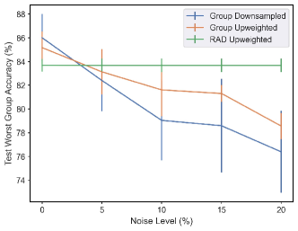
(a) CelebA

(b) MultiNLI

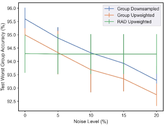
(c) CMNIST

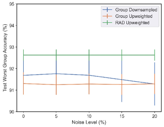
(d) Waterbirds

Figure 4: We compare the worst group accuracy of the domain annotation-dependent methods with RAD-UW, which is independent of domain annotations. (a) For CelebA, at just $5\%$ noise, RAD-UW outperforms both the domain-annotation dependent methods. (b) For MultiNLI, at $5\%$ noise, RAD-UW matches both the domain-annotation dependent methods and outperforms them at higher noise levels. (c) For CMNIST, at $10\%$ noise, RAD-UW matches Group Downsampled and outperforms both the domain-dependent methods at higher noise levels. (d) For Waterbirds, RAD-UW outperforms both the domain-dependent methods at every noise level.

References

- Arjovsky et al. (2019) Arjovsky, M., Bottou, L., Gulrajani, I., and Lopez-Paz, D. Invariant risk minimization. arXiv preprint arXiv:1907.02893, 2019.
- Chaudhuri et al. (2023) Chaudhuri, K., Ahuja, K., Arjovsky, M., and Lopez-Paz, D. Why does throwing away data improve worst-group error? In Proceedings of the 40th International Conference on Machine Learning, 2023.
- Giannone et al. (2021) Giannone, G., Havrylov, S., Massiah, J., Yilmaz, E., and Jiao, Y. Just mix once: Mixing samples with implicit group distribution. In NeurIPS 2021 Workshop on Distribution Shifts, 2021.
- Idrissi et al. (2022) Idrissi, B. Y., Arjovsky, M., Pezeshki, M., and Lopez-Paz, D. Simple data balancing achieves competitive worst-group-accuracy. In Proceedings of the First Conference on Causal Learning and Reasoning, 2022.
- Izmailov et al. (2022) Izmailov, P., Kirichenko, P., Gruver, N., and Wilson, A. G. On feature learning in the presence of spurious correlations. Advances in Neural Information Processing Systems, 2022.
- Kirichenko et al. (2023) Kirichenko, P., Izmailov, P., and Wilson, A. G. Last layer re-training is sufficient for robustness to spurious correlations. In The Eleventh International Conference on Learning Representations, 2023.
- LaBonte et al. (2023) LaBonte, T., Muthukumar, V., and Kumar, A. Towards last-layer retraining for group robustness with fewer annotations. In Conference on Neural Information Processing Systems (NeurIPS), 2023.
- Liu et al. (2021) Liu, E. Z., Haghgoo, B., Chen, A. S., Raghunathan, A., Koh, P. W., Sagawa, S., Liang, P., and Finn, C. Just train twice: Improving group robustness without training group information. In Proceedings of the 38th International Conference on Machine Learning, 2021.
- Liu et al. (2015) Liu, Z., Luo, P., Wang, X., and Tang, X. Deep learning face attributes in the wild. In Proceedings of International Conference on Computer Vision (ICCV), 2015.
- Oh et al. (2022) Oh, D., Lee, D., Byun, J., and Shin, B. Improving group robustness under noisy labels using predictive uncertainty. ArXiv, abs/2212.07026, 2022.
- Oren et al. (2019) Oren, Y., Sagawa, S., Hashimoto, T. B., and Liang, P. Distributionally robust language modeling. In Proceedings of the 2019 Conference on Empirical Methods in Natural Language Processing and the 9th International Joint Conference on Natural Language Processing (EMNLP-IJCNLP), 2019.
- Patrini et al. (2017) Patrini, G., Rozza, A., Krishna Menon, A., Nock, R., and Qu, L. Making deep neural networks robust to label noise: A loss correction approach. In Proceedings of the IEEE conference on computer vision and pattern recognition, 2017.
- Pedregosa et al. (2011) Pedregosa, F., Varoquaux, G., Gramfort, A., Michel, V., Thirion, B., Grisel, O., Blondel, M., Prettenhofer, P., Weiss, R., Dubourg, V., Vanderplas, J., Passos, A., Cournapeau, D., Brucher, M., Perrot, M., and Duchesnay, E. Scikit-learn: Machine learning in Python. Journal of Machine Learning Research, 2011.
- Qiu et al. (2023) Qiu, S., Potapczynski, A., Izmailov, P., and Wilson, A. G. Simple and fast group robustness by automatic feature reweighting. In Proceedings of the 40th International Conference on Machine Learning, 2023.
- Sagawa et al. (2020) Sagawa, S., Koh, P. W., Hashimoto, T. B., and Liang, P. Distributionally robust neural networks. In International Conference on Learning Representations, 2020.
- Wei et al. (2022) Wei, J., Zhu, Z., Cheng, H., Liu, T., Niu, G., and Liu, Y. Learning with noisy labels revisited: A study using real-world human annotations. In International Conference on Learning Representations, 2022.
- Williams et al. (2018) Williams, A., Nangia, N., and Bowman, S. A broad-coverage challenge corpus for sentence understanding through inference. In Proceedings of the 2018 Conference of the North American Chapter of the Association for Computational Linguistics: Human Language Technologies, Volume 1 (Long Papers), 2018.
- Yang et al. (2023) Yang, Y., Zhang, H., Katabi, D., and Ghassemi, M. Change is hard: A closer look at subpopulation shift. In International Conference on Machine Learning, 2023.
- Yao et al. (2022) Yao, H., Wang, Y., Li, S., Zhang, L., Liang, W., Zou, J., and Finn, C. Improving out-of-distribution robustness via selective augmentation. In Proceedings of the 39th International Conference on Machine Learning, 2022.