The Primordial Black Hole Abundance: The Broader, the Better

Abstract

We show that the abundance of primordial black holes, if formed through the collapse of large fluctuations generated during inflation and unless the power spectrum of the curvature perturbation is very peaked, is always dominated by the broadest profile of the compaction function, even though statistically it is not the most frequent. The corresponding threshold is therefore 2/5. This result exacerbates the tension when combining the primordial black hole abundance with the signal seen by pulsar timing arrays and originated from gravitational waves induced by the same large primordial perturbations.

1 Introduction and Conclusions

Primordial Black Holes (PBHs) have emerged as one of the most interesting topics in cosmology in the last years (see Ref. [1] for a recent review). PBHs could explain both some of the signals from binary black hole mergers observed in gravitational wave detectors [2] and be an important component of the dark matter in the Universe.

One of the crucial parameter in PBHs physics is the relative abundance of PBHs with respect to the dark matter component. This quantity is not easy to calculate in the scenario in which PBHs are formed by the collapse of large fluctuations generated during inflation upon horizon re-entry. Indeed, the formation probability is very sensitive to tiny changes in the various ingredients, such as the critical threshold of collapse, the non-Gaussian nature of the fluctuations, the choice of the window function to define smoothed observables (see again Ref. [1] for a nice discussion on such issues), the nonlinear corrections entering in the calculation of the PBHs abundance from the nonlinear radiation transfer function and the determination of the true physical horizon crossing [3] and the appearance of an infinite tower of local, non-local and higher-derivative operators upon dealing with the nonlinear overdensity [4].

One intrinsic and therefore unavoidable source of uncertainty in calculating the PBHs abundance arises from the inability to predict the value of a given observable with zero uncertainty, e.g. the compaction function or its curvature at its peak, in a given point or region. This is due to the fact that the theory delivers only stochastic quantities, e.g. the curvature perturbation, of which we know only the power spectrum and the higher-order correlators. Therefore, we are allowed to calculate only ensemble averages and typical values, which come with intrinsic uncertainties quantified by, for example, root mean square deviations.

Since the critical PBHs abundance depends crucially on the curvature of the compaction function at its peak, the natural question which arises is the following: in order to calculate the PBHs abundance, which value of the critical threshold should we use? In other words, which value of the curvature should one adopt to derive the formation threshold?

A natural answer to this question might be to use the average profile of the compaction function, and this is done routinely in the literature. After all, most of the Hubble volumes are populated by peaks with such average profile at horizon re-entry.

In this paper we wish to make a simple, but relevant observation: only if the power spectrum of the curvature perturbation is very peaked, the critical threshold for formation is determined by the average value of the curvature of the compaction function at the peak; in the realistic cases in which the power spectrum of the curvature perturbation is not peaked, the critical threshold for formation is determined by the broadest possible compaction function. This is because the abundance is dominated by the smallest critical threshold, which corresponds to the broadest profile. In such a case, the threshold for the compaction function is fixed to be 2/5.

This paper is organized as follows. In section 2 we briefly summarize the properties of the compaction function; in sections 3 and 4 we prove our observation, while in section 5 we make a comparison with the recent literature and its implication with Pulsar Timing Arrays experiments. In section 6 we provide some final comments.

2 The compaction function

The key starting object is the curvature perturbation $\zeta(\bf x)$ on superhorizon scales which appears in the metric in the comoving uniform-energy density gauge

$${\rm d}s^{2}=-{\rm d}t^{2}+a^{2}(t)e^{2\zeta(\bf x)}{\rm d}{\bf x}^{2},$$ (2.1)

where $a(t)$ is the scale factor in terms of cosmic time. Cosmological perturbations may gravitationally collapse to form a PBH depending on the amplitude measured at the peak of the compaction function, defined as the mass excess compared to the background value within a given radius (see for instance Ref. [5])

$$C({\bf x})=2\frac{M({\bf x},t)-M_{\rm b}({\bf x},t)}{R({\bf x},t)},$$ (2.2)

where $M({\bf x},t)$ is the Misner-Sharp mass and $M_{\rm b}({\bf x},t)$ its background value. The Misner-Sharp mass gives the mass within a sphere of areal radius

$$R({\bf x},t)=a(t)re^{\zeta(\bf x)}$$ (2.3)

with spherical coordinate radius $r$, centered around position ${\bf x}$ and evaluated at time $t$. The compaction directly measures the overabundance of mass in a region and is therefore better suited than the curvature perturbation for determining when an overdensity collapses into a PBH. Furthermore, the compaction has the advantage to be time-independent on superhorizon scales. It can be written in terms of the density contrast as

$$C({\bf x})=\frac{2\rho_{\rm b}}{R({\bf x},t)}\int{\rm d}^{3}{\bf x}\,\delta({\bf x},t),$$ (2.4)

where $\rho_{\rm b}$ is the background energy density. On superhorizon scales the density contrast is related to the curvature perturbation in real space by the nonlinear relation

$$\delta({\bf x},t)=-\frac{4}{9}\frac{1}{a^{2}H^{2}}e^{-2\zeta(\bf x)}\left(\nabla^{2}\zeta({\bf x})+\frac{1}{2}\left({\mathbf{\nabla}}\zeta({\bf x})\right)^{2}\right).$$ (2.5)

Assuming spherical symmetry and defining $\zeta^{\prime}={\rm d}\zeta/{\rm d}r$, the compaction function becomes

$$C(r) = \frac{8\pi\rho_{\rm b}}{R(r,t)}\int_{0}^{R}{\rm d}\widetilde{R}\,\widetilde{R}^{2}(r,t)\delta(r,t)=C_{\zeta}(r)-\frac{3}{8}C_{\zeta}^{2}(r),$$

$$C_{\zeta}(r) = -\frac{4}{3}r\zeta^{\prime}(r).$$ (2.6)

Suppose now that there is peak in the curvature perturbation $\zeta({\bf x})$ with a given peak value $\zeta(0)$ and profile $\zeta(r)$ away from the center, which we arbitrarily can set at the origin of the coordinates. The corresponding compaction function will have a maximum at the distance $r_{m}$ from the origin of the peak. Since

$$C^{\prime}(r_{m})=C^{\prime}_{\zeta}(r_{m})\left[1-\frac{3}{4}C_{\zeta}(r_{m})\right]=0,$$ (2.7)

the extremum of the compaction function $C(r)$ coincides with the extremum of $C_{\zeta}(r)$. Furthermore, since

$$C^{\prime\prime}(r_{m})=C^{\prime\prime}_{\zeta}(r_{m})\left[1-\frac{3}{4}C_{\zeta}(r_{m})\right],$$ (2.8)

the maximum of the compaction function $C(r)$ coincides with the maximum of $C_{\zeta}(r)$ as long as $C_{\zeta}(r_{m})<4/3$ (the so-called type I case). We will focus therefore mainly on this quantity. Notice that sometimes we will call $C_{\zeta}(r)$ “linear” compaction function for simplicity, where the term linear stems from the fact that its expression is linear in the curvature perturbation $\zeta(r)$. However, $C_{\zeta}(r)$ is not necessarily Gaussian if the curvature perturbation $\zeta(r)$ is not.

The maximum of the compaction function is fixed by the equation

$$C^{\prime}(r_{m})=C^{\prime}_{\zeta}(r_{m})=0\,\,\,\,{\rm or}\,\,\,\,\zeta^{\prime}(r_{m})+r_{m}\zeta^{\prime\prime}(r_{m})=0.$$ (2.9)

Consider now a family of compaction functions which have in common the same value of $r_{m}$, but a different curvature at the maximum parametrized by [6]

$$q=-\frac{1}{4}\frac{r_{m}^{2}C^{\prime\prime}(r_{m})}{C(r_{m})},$$ (2.10)

Numerically, it has been noticed that the critical threshold depends on the curvature at the peak of the compaction function [6, 7, 8]

$$C_{c}(q)=\frac{4}{15}e^{-1/q}\frac{q^{1-5/2q}}{\Gamma(5/2q)-\Gamma(5/2q,1/q)},$$ (2.11)

such that $C_{c}(q\ll 1)\simeq 2/5$ and $C_{c}(q\gg 1)\simeq 2/3$. We also notice that

$$q=-\frac{1}{4}\frac{r_{m}^{2}C_{\zeta}^{\prime\prime}(r_{m})\left[1-\frac{3}{4}C_{\zeta}(r_{m})\right]}{C_{\zeta}(r_{m})\left[1-\frac{3}{8}C_{\zeta}(r_{m})\right]}\simeq-\frac{1}{4}\frac{r_{m}^{2}C_{\zeta}^{\prime\prime}(r_{m})}{C_{\zeta}(r_{m})}\left[1-\frac{3}{8}C_{\zeta}(r_{m})\right]\equiv q_{\zeta}\left[1-\frac{3}{8}C_{\zeta}(r_{m})\right].$$ (2.12)

2.1 The average profile

One question to pose is the following: which profile should one make use of to calculate the critical value for PBH abundance, given that it depends on the peak profile? The natural answer, routinely adopted in the literature, would be the average profile of the compaction function with the constraint that there is a peak of the curvature perturbation at the center of the coordinates with value $\zeta(0)$. This is the most obvious answer as the average profile is the most frequent, statistically speaking. Supposing for the moment that $\zeta(r)$ is Gaussian, such an average profile would be

$$\langle C_{\zeta}(r)\rangle_{\zeta(0)}=-\frac{4}{3}r\langle\zeta^{\prime}(r)\rangle_{\zeta(0)}=-\frac{4}{3}r\langle\zeta(r)\rangle_{\zeta(0)}^{\prime}=-\frac{4}{3}r\frac{\xi^{\prime}(r)}{\xi(0)}\zeta_{0},$$ (2.13)

where

$$\xi(r)=\int\frac{{\rm d}k}{k}{\cal P}_{\zeta}(k)\frac{\sin kr}{kr}$$ (2.14)

is the two-point correlation of the curvature perturbation. In such a case the value of $r_{m}$ where the most likely compaction function has its maximum would then be fixed by the equation

$$\xi^{\prime}(r_{m})+r_{m}\xi^{\prime\prime}(r_{m})=0.$$ (2.15)

A standard choice is therefore to calculate the curvature of the peak of the compaction function as

$$q=-\frac{1}{4}\frac{r_{m}^{2}\langle C^{\prime\prime}_{\zeta}(r_{m})\rangle_{\zeta(0)}}{\langle C_{\zeta}(r_{m})\rangle_{\zeta(0)}}\left[1-\frac{3}{8}\langle C_{\zeta}(r_{m})\rangle_{\zeta(0)}\right].$$ (2.16)

The crucial point is that, the smaller the value of the curvature, the smaller the value of the threshold. Since the PBHs abundance has an exponentially strong dependence on the threshold, one expects that broad compaction functions should be very relevant in the determination of the abundance of PBHs even though they are more rare than the average profiles. This is what we discuss next.

3 The relevance of Broadness: the Gaussian case

In this section we assume $C_{\zeta}(r_{m})$ and $C_{\zeta}^{\prime\prime}(r_{m})$ to be Gaussian (and correlated) variables. This will allow us to gain some analytical intuition. We define

$$\sigma^{2}_{0}=\langle C_{\zeta}^{2}(r_{m})\rangle,\,\,\,\sigma^{2}_{1}=-\frac{1}{4}r_{m}^{2}\langle C_{\zeta}^{\prime\prime}(r_{m})C_{\zeta}(r_{m})\rangle,\,\,\,{\rm and}\,\,\,\sigma^{2}_{2}=\frac{1}{16}r_{m}^{4}\langle{C_{\zeta}^{\prime\prime}(r_{m})}^{2}\rangle.$$ (3.1)

Such correlations are easily computed knowing that the Fourier transform of the linear compaction function reads

$$C_{\zeta}({\bf k},r)=\frac{4}{9}k^{2}r^{2}W(kr)\zeta({\bf k}),\,\,\,\,W(x)=3\frac{\sin x-x\cos x}{x^{3}},$$ (3.2)

where $W(x)$ is the Fourier transform of the Heaviside window function in real space. We will use the conservation of the probabilities

$$P\left[C(r_{m}),C^{\prime\prime}(r_{m})\right]{\rm d}C(r_{m}){\rm d}C^{\prime\prime}(r_{m}) = {\cal P}\left[C_{\zeta}(r_{m}),C_{\zeta}^{\prime\prime}(r_{m})\right]{\rm d}C_{\zeta}(r_{m}){\rm d}C_{\zeta}^{\prime\prime}(r_{m})$$ (3.3)

$$= \widetilde{{\cal P}}\left[C_{\zeta}(r_{m}),q_{\zeta}\right]{\rm d}C_{\zeta}(r_{m}){\rm d}q_{\zeta}$$

where

$${\cal P}\left[-\frac{1}{4}r_{m}^{2}C_{\zeta}^{\prime\prime}(r_{m}),C_{\zeta}(r_{m})\right] = \frac{1}{2\pi\sqrt{{\rm det}\,\Sigma}}\,{\rm exp}\left(-\vec{V}^{T}\Sigma^{-1}\vec{V}/2\right),$$

$$\vec{V}^{T} = \left[-\frac{1}{4}r_{m}^{2}C_{\zeta}^{\prime\prime}(r_{m}),C_{\zeta}(r_{m})\right],$$

$$\Sigma = \left(\begin{array}[]{cc}\sigma^{2}_{2}&\sigma^{2}_{1}\\ \sigma^{2}_{1}&\sigma^{2}_{0}\end{array}\right).$$ (3.6)

We find it convenient to define the parameter

$$\gamma=\frac{\sigma_{1}^{2}}{\sigma_{2}\sigma_{0}},$$ (3.7)

which will play an important role in the following and indicates the broadness of a given power spectrum of the curvature perturbation. The closer $\gamma$ is to unity, the more spiky is the peak of the curvature perturbation.

3.1 The average of the curvature

The average curvature of the linear compaction function $C_{\zeta}$ can be computed by using the conditional probability to have a peak at $r_{m}$

$$\langle q_{\zeta}\rangle=\int_{0}^{\infty}{\rm d}q_{\zeta}\,q_{\zeta}\,P[q|C_{\zeta}(r_{m})>C_{\zeta,c}(q_{\zeta})],$$ (3.8)

with

$$P[q|C_{\zeta}(r_{m})>C_{\zeta,c}(q_{\zeta})]=\frac{\widetilde{{\cal P}}[q_{\zeta},C_{\zeta}(r_{m})>C_{\zeta,c}(q_{\zeta})]}{\widetilde{{\cal P}}[C_{\zeta}(r_{m})>C_{\zeta,c}(q_{\zeta})]}.$$ (3.9)

The conditional probability, in the limit of large thresholds, becomes

$$P[q_{\zeta}|C_{\zeta}(r_{m})>C_{\zeta,c}(q_{\zeta})] \simeq \frac{\left(1-\gamma^{2}\right)^{1/2}\sigma_{2}C_{\zeta,c}(q_{\zeta})}{\sqrt{2\pi}\sigma_{0}\left[(q_{\zeta}-\gamma\sigma_{2}/\sigma_{0})^{2}+(1-\gamma^{2})\sigma_{2}^{2}/\sigma_{0}^{2}\right]^{1/2}}\cdot$$ (3.10)

$$\cdot \exp\left[-\frac{(q-\gamma\sigma_{2}/\sigma_{0})^{2}C^{2}_{\zeta,c}(q_{\zeta})}{2(1-\gamma^{2})\sigma_{2}^{2}}\right].$$

For a monochromatic power spectrum of the curvature perturbation, that is $\gamma\simeq 1$, we recognize the Dirac delta and the value of $q_{\zeta}$, which minimizes the exponent and maximizes the PBHs abundance, is the average value $\langle q_{\zeta}\rangle=\sigma_{2}/\sigma_{0}$.

Departing from $\gamma\simeq 1$, and integrating numerically, one discovers departures from the value $\gamma\sigma_{2}/\sigma_{0}$ for the average of $q_{\zeta}$, but not dramatically, and one has

$$\langle q_{\zeta}\rangle\simeq\gamma\frac{\sigma_{2}}{\sigma_{0}}.$$ (3.11)

3.2 The PBHs abundance

The PBHs abundance is given by

$$\beta=\int_{C_{c}(q)}^{\infty}{\rm d}C(r_{m})\int_{-\infty}^{0}{\rm d}C^{\prime\prime}(r_{m})P\left[C(r_{m}),C^{\prime\prime}(r_{m})\right]=\int_{0}^{\infty}{\rm d}q_{\zeta}\int_{C_{\zeta,c}(q_{\zeta})}^{\infty}{\rm d}C_{\zeta}(r_{m})\widetilde{{\cal P}}\left[C_{\zeta}(r_{m}),q_{\zeta}\right].$$ (3.12)

Going back to the initial probability, it can be written as

$${\cal P}\left[-\frac{1}{4}r_{m}^{2}C_{\zeta}^{\prime\prime}(r_{m}),C_{\zeta}(r_{m})\right] = \frac{1}{2\pi}\frac{1}{\sigma_{2}\sigma_{0}\sqrt{1-\gamma^{2}}}{\rm exp}\left[-\frac{r_{m}^{4}{C_{\zeta}^{\prime\prime}(r_{m})}^{2}}{16\cdot 2\sigma_{2}^{2}}\right]\cdot$$ (3.13)

$$\cdot {\rm exp}\left[-\frac{1}{2(1-\gamma^{2})}\left(\frac{C_{\zeta}(r_{m})}{\sigma_{0}}+\gamma\frac{r_{m}^{2}C_{\zeta}^{\prime\prime}(r_{m})}{4\sigma_{2}}\right)^{2}\right].$$

For a monochromatic, very peaked, power spectrum of the curvature perturbation, where $\gamma\simeq 1$, the probability reduces to

$$\lim_{\gamma\rightarrow 1}{\cal P}\left[-\frac{1}{4}r_{m}^{2}C_{\zeta}^{\prime\prime}(r_{m}),C_{\zeta}(r_{m})\right]=\frac{1}{\sqrt{2\pi}}\frac{1}{\sigma_{2}\sigma_{0}}{\rm exp}\left(-\frac{r_{m}^{4}{C_{\zeta}^{\prime\prime}(r_{m})}^{2}}{16\cdot 2\sigma_{2}^{2}}\right)\delta_{D}\left(\frac{C_{\zeta}(r_{m})}{\sigma_{0}}+\frac{r_{m}^{2}C_{\zeta}^{\prime\prime}(r_{m})}{4\sigma_{2}}\right),$$ (3.14)

which fixes

$$q_{\zeta}=\frac{\sigma_{2}}{\sigma_{0}}=\frac{\sigma_{2}\sigma_{0}}{\sigma_{0}^{2}}=\frac{\sigma^{2}_{1}}{\sigma^{2}_{0}}=\langle q_{\zeta}\rangle,$$ (3.15)

and

$$\beta = \int_{0}^{\infty}{\rm d}q_{\zeta}\int_{C_{\zeta,c}(q_{\zeta})}^{4/3}{\rm d}C_{\zeta}(r_{m}){\cal P}\left[-\frac{1}{4}r_{m}^{2}C_{\zeta}^{\prime\prime}(r_{m}),C_{\zeta}(r_{m})\right]$$ (3.16)

$$= \int_{C_{\zeta,c}(\langle q_{\zeta}\rangle)}^{4/3}{\rm d}C_{\zeta}(r_{m})\frac{1}{\sqrt{2\pi}\sigma_{0}}{\rm exp}\left(-\frac{C^{2}_{\zeta}(r_{m})}{2\sigma_{0}^{2}}\right)=\frac{1}{2}{\rm Erfc}\left[\frac{C_{\zeta,c}(\langle q_{\zeta}\rangle)}{\sqrt{2}\sigma_{0}}\right],$$

where

$$C_{\zeta,c}(q_{\zeta})\simeq\frac{4}{3}\left(1-\sqrt{\frac{2-3C_{c}(q_{\zeta})}{2}}\right).$$ (3.17)

Therefore for monochromatic spectra of the curvature perturbation the PBHs abundance is fixed by the value of the threshold corresponding to the average value of the curvature of the compaction function at its peak

$$C^{\rm peaked}_{\zeta,c}=C_{\zeta,c}(\langle q_{\zeta}\rangle).$$ (3.18)

For a generic power spectrum, we change the variables from $(-r_{m}^{2}C_{\zeta}^{\prime\prime}(r_{m}),C_{\zeta}(r_{m}))$ to $(q_{\zeta},C_{\zeta}(r_{m}))$ and making use of the conservation of the probability we obtain

$$\beta(q_{\zeta}) = \int_{C_{\zeta,c}(q_{\zeta})}^{4/3}{\rm d}C_{\zeta}(r_{m})|C_{\zeta}(r_{m})|\,{\cal P}\left[qC_{\zeta}(r_{m}),C_{\zeta}(r_{m})\right]$$

$$\simeq \frac{\sqrt{1-\gamma^{2}}\sigma_{2}}{2\pi\sigma_{0}\left[(q_{\zeta}-\gamma\sigma_{2}/\sigma_{0})^{2}+(1-\gamma^{2})\sigma^{2}_{2}/\sigma^{2}_{0}\right]}\cdot$$

$$\cdot \exp\left[-\frac{\left[(q_{\zeta}-\gamma\sigma_{2}/\sigma_{0})^{2}+(1-\gamma^{2})\sigma^{2}_{2}/\sigma^{2}_{0}\right]C^{2}_{\zeta,c}(q_{\zeta})}{2(1-\gamma^{2})\sigma^{2}_{2}}\right].$$

We see that the square of the critical threshold is replaced by an effective squared critical threshold

$$C^{2}_{\zeta,c}(q_{\zeta})\Big{|}_{\rm eff}=\left[(q_{\zeta}-\gamma\sigma_{2}/\sigma_{0})^{2}+(1-\gamma^{2})\sigma_{2}^{2}/\sigma_{0}^{2}\right]C^{2}_{\zeta,c}(q_{\zeta}).$$ (3.20)

Its minimum is determined by the equation

$$(q_{\zeta}-\gamma\sigma_{2}/\sigma_{0})C_{\zeta,c}(q_{\zeta})+\left[(q_{\zeta}-\gamma\sigma_{2}/\sigma_{0})^{2}+(1-\gamma^{2})\sigma_{2}^{2}/\sigma_{0}^{2}\right]\frac{{\rm d}C_{\zeta,c}(q_{\zeta})}{{\rm d}q_{\zeta}}=0.$$ (3.21)

For peaked profiles where $\gamma\simeq 1$ we have

$$(q_{\zeta}-\sigma_{2}/\sigma_{0})\left[C_{\zeta,c}(q_{\zeta})+(q_{\zeta}-\sigma_{2}/\sigma_{0})\frac{{\rm d}C_{\zeta,c}(q_{\zeta})}{{\rm d}q_{\zeta}}\right]=0$$ (3.22)

and the mimimum lies at the value of the average $q_{\zeta}=\langle q_{\zeta}\rangle=\sigma_{2}/\sigma_{0}$. For broad spectra $\gamma\ll 1$, the effective threshold is minimized for $q_{\zeta}\simeq 0$ as it reduces to

$$C^{2}_{\zeta,c}(q_{\zeta})\Big{|}_{\rm eff}=\left[q_{\zeta}^{2}+\sigma_{2}^{2}/\sigma_{0}^{2}\right]C^{2}_{\zeta,c}(q_{\zeta}).$$ (3.23)

and the threshold $C_{\zeta,c}(q_{\zeta})$ is also minimized for small $q_{\zeta}$. There is in general a critical value of $q_{\zeta}$ for which the abundance is always dominated by the broad spectra. We can see this behaviour by plotting the curve $(q_{\zeta\;\rm{min}},\gamma)$ obtain from the Eq. (3.21), as shown in Fig. 2. As we start decreasing from $\gamma=1$ where the minimum is in $\sigma_{2}/\sigma_{0}$, also the value of $q_{\zeta,\;\rm{min}}$ decreases, up until a critical value $\gamma_{\rm crit}$. For values of $\gamma$ below this point the function $C_{\zeta,c}(q_{\zeta})|_{\rm{eff}}$ does not have a minimum, but is monotonically increasing with $q_{\zeta}$, hence the minimum lies at the boundary of the interval, i.e. $q_{\zeta}=0$. The transition is therefore very sharp after the critical value.
It is also possible to evaluate the position of this minimum for different values of the parameter $\sigma_{2}/\sigma_{0}$, as shown in Fig. 2. We can understand the behaviour because having larger values of this parameter the transition happens for larger values of $\gamma$, being easier to enter in the regime of Eq. (3.23), where $\sigma_{2}/\sigma_{0}$ dominates.

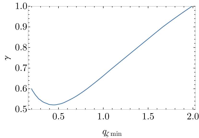
Figure 1: Plot of $q_{\zeta\;\rm{\min}}$ as a function of $\gamma$ for $\sigma_{2}/\sigma_{0}=2$.

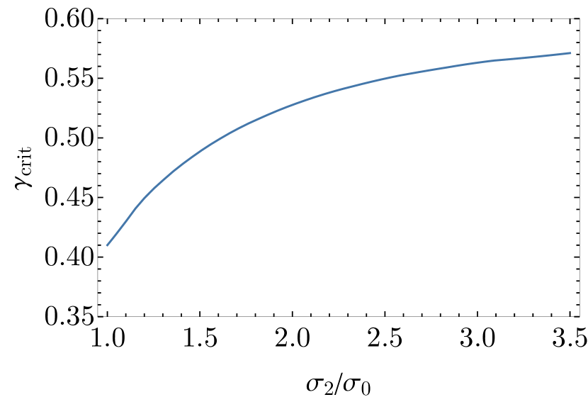
Figure 2: Critical value of $\gamma$ as a function of $\sigma_{2}/\sigma_{0}$

To show this explicitly, in Fig. 3 we plot the formation probability for three different values of $\gamma$. It demonstrates that the abundance is dominated by the broadest profiles when the curvature perturbation is not very spiky and not by the average value of $q_{\zeta}$. The corresponding critical value needed to be used is therefore

$$C_{\zeta,c}(q_{\zeta}\simeq 0)\simeq\frac{4}{3}\left(1-\sqrt{\frac{2-3\cdot 2/5}{2}}\right)\simeq 0.49.$$ (3.24)

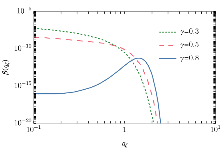
Figure 3: The PBHs formation probability as a function of $q_{\zeta}$ for $\sigma_{0}=\sigma_{2}/2=0.05$ and three different values of $\gamma=(0.3,0.5,0.8)$ for which $\langle q_{\zeta}\rangle=(0.6,1,1.6)$ for the Gaussian case.

4 The relevance of Broadness: the non-Gaussian case

As a matter of fact, the curvature perturbation generated in models producing large overdensities is typically non-Gaussian. Non-Gaussianity among the modes interested in the growth of the curvature perturbation is generated either by their self-interaction during the ultra slow-roll phase [10] or after Hubble radius exit when the curvature perturbation is sourced by a curvaton-like field [11, 12, 13].

We proceed therefore by assuming that the initial curvature perturbation is non-Gaussian, but a function of a Gaussian component

$$\zeta(r)=F[\zeta_{\rm g}(r)].$$ (4.1)

In such a case the compaction function is still given by Eq. (2), where

$$C_{\zeta}(r)=F_{1}(\zeta_{\rm g})C_{\rm g}(r),\,\,\,\,C_{\rm g}(r)=-\frac{4}{3}r\zeta^{\prime}_{\rm g}(r),$$ (4.2)

and we have indicated the derivatives of $F$ with respect to $\zeta_{\rm g}$ by $F_{n}={\rm d}F(\zeta_{\rm g})/{\rm d}\zeta_{\rm g}$. The maximum of the compaction function can be found solving the equation

$$C_{\zeta}^{\prime}(r_{m})=F_{1}(\zeta_{\rm g})C^{\prime}_{{\rm g}}(r_{m})+C_{{\rm g}}(r_{m})\zeta_{\rm g}^{\prime}(r_{m})F_{2}(\zeta_{\rm g})=0,$$ (4.3)

as long as $C_{\zeta}(r_{m})<4/3$. The next step is to define the following Gaussian and correlated variables

$$x_{0}=\zeta_{\rm g},\quad x_{1}=r\zeta^{\prime}_{\rm g},\quad x_{2}=r^{2}\zeta^{\prime\prime}_{\rm g},\quad x_{3}=r^{3}\zeta^{\prime\prime\prime}_{\rm g},$$ (4.4)

for which the condition of the maximum becomes

$$x_{2}=-x_{1}\left(1+x_{1}\frac{F_{2}(x_{0})}{F_{1}(x_{0})}\right).$$ (4.5)

One can construct the corresponding probability distribution as

$$P(x_{0},x_{1},x_{2},x_{3})=\frac{1}{(2\pi)^{2}\sqrt{{\rm det}\,\Sigma}}\,{\rm exp}\left(-\vec{V}^{T}\Sigma^{-1}\vec{V}/2\right),$$ (4.6)

where

$$\vec{V}^{T}=\left[x_{0},x_{1},x_{2},x_{3}\right],$$

and

$$\Sigma = \left(\begin{array}[]{cccc}\sigma^{2}_{0}&\gamma_{01}\sigma_{1}\sigma_{0}&\gamma_{02}\sigma_{2}\sigma_{0}&\gamma_{03}\sigma_{3}\sigma_{0}\\ \gamma_{01}\sigma_{1}\sigma_{0}&\sigma_{1}^{2}&\gamma_{12}\sigma_{2}\sigma_{1}&\gamma_{13}\sigma_{1}\sigma_{3}\\ \gamma_{02}\sigma_{2}\sigma_{0}&\gamma_{12}\sigma_{2}\sigma_{1}&\sigma^{2}_{2}&\gamma_{23}\sigma_{2}\sigma_{3}\\ \gamma_{03}\sigma_{3}\sigma_{0}&\gamma_{13}\sigma_{1}\sigma_{3}&\gamma_{23}\sigma_{2}\sigma_{3}&\sigma_{3}^{2}\end{array}\right)$$ (4.11)

is constructed from the different correlators with

$$\sigma_{i}^{2}=\langle x_{i}^{2}\rangle,\quad\gamma_{ij}=\frac{\langle x_{i}x_{j}\rangle}{\langle x_{i}^{2}\rangle^{1/2}\;\langle x_{j}^{2}\rangle^{1/2}}.$$ (4.12)

Next, we need to convert all the relevant variables in terms of the Gaussian ones $x_{i}$ ($i=0,\cdots,3)$. First we have

$$C_{{\rm g}}=-\frac{4}{3}\,x_{1},$$ (4.13)

and the derivatives of $C_{\zeta}$ can be written in terms of $x_{1}$ and $x_{2}$ as

$$C_{\zeta} = -\frac{4}{3}\;x_{1}F_{1}(x_{0}),$$

$$rC_{\zeta}^{\prime} = -\frac{4}{3}\left(F_{1}(x_{0})(x_{1}+x_{2})+x_{1}^{2}F_{2}(x_{0})\right),$$

$$r^{2}C_{\zeta}^{\prime\prime} = -\frac{4}{3}\left[F_{1}(x_{0})(2x_{2}+x_{3})+2x_{1}^{2}F_{2}(x_{0})+3x_{1}x_{2}F_{2}(x_{0})+x_{1}^{3}F_{3}(x_{0})\right].$$ (4.14)

The PBHs abundance for a given value of the curvature $q$ will read

$$\beta(q)=\int_{D}\mathcal{K}\left(C-C_{c}(q)\right)^{\gamma}\;p(x_{0},C_{\zeta},x_{2},q)\;\delta\left(F_{1}(x_{0})(x_{1}+x_{2})+x_{1}^{2}F_{2}(x_{0})\right),$$ (4.15)

where the domain of integration is

$$D=\left\{x_{2}\in\mathbb{R},C_{\zeta,c}(q)<C_{\zeta}<\frac{4}{3}\right\},$$ (4.16)

with

$$C_{\zeta,c}(q)\simeq\frac{4}{3}\left(1-\sqrt{\frac{2-3C_{c}(q)}{2}}\right).$$ (4.17)

We have reintroduced the scaling-law factor for critical collapse $\mathcal{K}(C-C_{c}(q))^{\gamma}$ which accounts for the mass of the PBHs at formation written in units of the horizon mass at the time of horizon re-entry, with $\mathcal{K}\simeq 3.3$ for a log-normal power spectrum and $\gamma\simeq 0.36$ [14, 15, 16] (see also Ref. [17]). By using the conservation of probabilities we can finally write

$$p\left[\zeta_{\rm g},C_{\zeta},x_{2},q\right]=P\left[x_{0},x_{1},x_{2},x_{3}\right]|{\rm Det}\,J|,$$ (4.18)

where

$${\rm Det}\,J=\frac{3}{4}\left(\frac{4x_{1}+2F_{1}(x_{0})x_{1}^{2}}{1+F_{1}(x_{0})x_{1}}\right),$$ (4.19)

and at the maximum

$$x_{3}=\frac{-4q(1+\frac{1}{2}x_{1}F_{1}(x_{0}))x_{1}}{1+x_{1}F_{1}(x_{0})}-2x_{2}-2x_{1}^{2}\frac{F_{2}(x_{0})}{F_{1}(x_{0})}-3x_{1}x_{2}\frac{F_{2}(x_{0})}{F_{1}(x_{0})}-x_{1}^{3}\frac{F_{3}(x_{0})}{F_{1}(x_{0})}.$$ (4.20)

We rewrite the Gaussian probability in the following form

$$P(x_{0},x_{1},x_{2},x_{3})=\frac{1}{4\pi^{2}\sqrt{\det{\Sigma}}}\exp{\left(-\frac{(\sigma_{0}\sigma_{1}\sigma_{2}\sigma_{3})^{2}}{2\det{\Sigma}}\sum_{i,j=0}^{3}\frac{\kappa_{ij}x_{i}x_{j}}{\sigma_{i}\sigma_{j}}\right)},$$ (4.21)

where the $\kappa_{ij}$’s will depend on all the $\gamma_{lm}$, and they can be computed by performing the inverse of the matrix $\Sigma$, matching with the definition. Performing the change of variables we get

$$p(\zeta_{\rm g},C_{\zeta},x_{2},q) = \left|\frac{9C_{\rm g}\left(3C_{\rm g}F_{1}-8\right)}{8\ \left(3C_{\rm g}F_{1}-4\right)}\right|\frac{1}{4\pi^{2}\sqrt{\det{\Sigma}}}\cdot$$

$$\cdot \exp{\left(-\frac{(\sigma_{0}\sigma_{1}\sigma_{2}\sigma_{3})^{2}}{2\det{\Sigma}}\frac{1}{4096\ F_{1}^{4}}\left[A(\zeta_{\rm g},C_{\rm g})q^{2}+B(\zeta_{\rm g},C_{\rm g})q+C(\zeta_{\rm g},C_{\rm g})\right]\right)},$$

where we have defined the following functions of $\zeta_{\rm g}$ and $C_{\rm g}$

$$A(\zeta_{\rm g},C_{\rm g})=\frac{9216\kappa_{33}C_{\rm g}^{2}F_{1}^{4}\left(8-3C_{\rm g}F_{1}\right){}^{2}}{\sigma_{3}^{2}\left(4-3C_{\rm g}F_{1}\right){}^{2}},$$ (4.23)

$$B(\zeta_{\rm g},C_{\rm g}) = \frac{192C_{\rm g}F_{1}^{2}\left(3C_{\rm g}F_{1}-8\right)}{\sigma_{0}\sigma_{1}\sigma_{2}\sigma_{3}^{2}\left(3C_{\rm g}F_{1}-4\right)}\left[3\kappa_{33}\sigma_{0}\sigma_{1}\sigma_{2}C_{\rm g}\left\{9C_{\rm g}F_{1}\left(C_{\rm g}F_{3}+4F_{2}\right)-27C_{\rm g}^{2}F_{2}^{2}-32F_{1}^{2}\right\}\right.$$ (4.24)

$$\left.+4\sigma_{3}F_{1}\left\{3\kappa_{23}\sigma_{0}\sigma_{1}C_{\rm g}\left(4F_{1}-3C_{\rm g}F_{2}\right)+4\sigma_{2}F_{1}\left(4\kappa_{30}\sigma_{1}\zeta_{\rm g}-3\kappa_{13}\sigma_{0}C_{\rm g}\right)\right\}\right],$$

$$C(\zeta_{\rm g},C_{\rm g}) = -\frac{\kappa_{33}}{\sigma_{3}^{2}}\left\{4374C_{\rm g}^{6}F_{1}F_{2}^{2}F_{3}-5832C_{\rm g}^{5}F_{1}^{2}F_{2}F_{3}+17496C_{\rm g}^{5}F_{1}F_{2}^{3}-27216C_{\rm g}^{4}F_{1}^{2}F_{2}^{2}+\right.$$

$$\left.20736C_{\rm g}^{3}F_{1}^{3}F_{2}-729C_{\rm g}^{6}F_{1}^{2}F_{3}^{2}+5184C_{\rm g}^{4}F_{1}^{3}F_{3}-9216C_{\rm g}^{2}F_{1}^{4}-6561C_{\rm g}^{6}F_{2}^{4}\right\}+$$

$$-\frac{1}{\sigma_{0}\sigma_{1}\sigma_{2}\sigma_{3}}24C_{\rm g}\ F_{1}\left(-9C_{\rm g}F_{1}\left(C_{\rm g}F_{3}+4F_{2}\right)+27C_{\rm g}^{2}F_{2}{}^{2}+32F_{1}^{2}\right)$$

$$\left(3\kappa_{23}\sigma_{0}\sigma_{1}C_{\rm g}\left(4F_{1}-3C_{\rm g}F_{2}\right)+4\sigma_{2}F_{1}\left(4\kappa_{30}\sigma_{1}\zeta_{\rm g}-3\kappa_{13}\sigma_{0}C_{\rm g}\right)\right)+$$

$$+16F_{1}^{2}\left(\frac{24C_{\rm g}F_{1}\left(3C_{\rm g}F_{2}-4F_{1}\right)\left(3\kappa_{12}\sigma_{0}C_{\rm g}-4\kappa_{20}\sigma_{1}\zeta_{\rm g}\right)}{\sigma_{0}\sigma_{1}\sigma_{2}}+\right.$$

$$\left.+\frac{9\kappa_{22}C_{\rm g}^{2}\ \left(4F_{1}-3C_{\rm g}F_{2}\right){}^{2}}{\sigma_{2}^{2}}+\frac{16F_{1}^{2}\left(-24\kappa_{10}\sigma_{1}\sigma_{0}C_{\rm g}\zeta_{\rm g}+9\kappa_{11}\sigma_{0}^{2}C_{\rm g}^{2}+16\kappa_{0}\sigma_{1}^{2}\zeta_{\rm g}^{2}\right)}{\sigma_{0}^{2}\sigma_{1}^{2}}\right),$$

and each function $F_{n}$ is intended to be $F_{n}(\zeta_{\rm g})$.

4.1 An illustrative example

We consider the following illustrative example which typically arises in models in which the curvature perturbation is generated during a period of ultra-slow-roll [10, 18, 19, 20]

$$\zeta({\bf x})=-\mu_{\star}\ln\left(1-\frac{\zeta_{\rm g}({\bf x})}{\mu_{\star}}\right),$$ (4.26)

with $\mu_{\star}$ a model-dependent parameter depending upon the transition between the ultra-slow-roll phase and the subsequent slow-roll phase. In this analysis we take $\mu_{\star}$ as a free parameter. We take the power spectrum of the Gaussian component to be a log-normal power spectrum

$${\cal P}_{\rm g}(k)=\frac{A}{\sqrt{2\pi}\Delta}{\rm exp}\left[-\ln^{2}(k/k_{\star})/2\Delta^{2}\right].$$ (4.27)

Our results are summarized in Fig. 4 where we have assumed $k_{\star}r_{m}=2$ for the plot. The broadness of the power spectrum is controlled by the parameter $\Delta$. We observe that by increasing the value of $\Delta$, enlarging the power spectra, again the PBHs formation probability is dominated by the broadest profiles. We have checked that for very peaked power spectrum, as in the case for $\Delta=1/3$, the abundance is peaked again around the average of $q$.

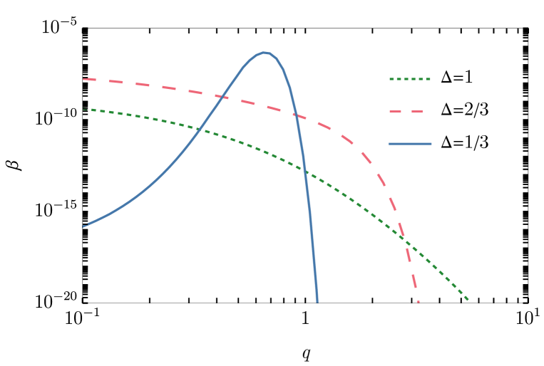
Figure 4: Mass fraction $\beta$ for the non-Gaussian scenario computed with several values of $\Delta$, where we fix $\mu_{*}=5/2$, $k_{*}r_{m}=2$ and the amplitude of the power spectrum $A=10^{-2}$.

5 Comparison with literature and impact on the physics of PBHs and Pulsar Timing Arrays

In this section we compare the calculation presented above, accounting for the curvature of the compaction function at its peak, with the prescription based on threshold statistics on the compaction function, reported in Refs. [23, 24], where the only explicit dependence on $q$ is encoded in $C_{c}(q)$. There, the formation probability is computed by integrating the joint probability distribution function $P_{\mathrm{g}}$

$$\beta=\int_{D}\mathcal{K}\left(C-C_{c}(q)\right)^{\gamma}\textrm{P}_{\rm g}(C_{\rm g},\zeta_{\rm g}){\rm d}C_{\rm g}{\rm d}\zeta_{\rm g}\,,$$ (5.1)

where the domain of integration is given by $\mathcal{D}=\left\{C(C_{\rm g},\zeta_{\rm g})>C_{\rm c}(q),~{}C_{\zeta}(C_{\rm g},\zeta_{\rm g})<4/3\right\}$. The Gaussian components are distributed as

$$P_{\rm g}\left(C_{\rm g},\zeta_{\rm g}\right)=\frac{1}{2\pi\sigma_{\rm a}\sigma_{\rm c}\sqrt{1-\gamma_{*}^{2}}}\exp\left[-\frac{1}{2\left(1-\gamma_{*}^{2}\right)}\left(\frac{C_{\mathrm{g}}}{\sigma_{\rm a}}-\frac{\gamma_{*}\zeta_{\mathrm{g}}}{\sigma_{\rm c}}\right)^{2}\!-\!\frac{\zeta_{\mathrm{g}}^{2}}{2\sigma_{\rm c}^{2}}\right],$$ (5.2)

with correlators

$$\langle C^{2}_{\rm g}\rangle =\sigma_{\rm a}^{2}=\frac{16}{81}\int_{0}^{\infty}\frac{{\rm d}k}{k}\left(kr_{m}\right)^{4}W^{2}\left(k,r_{m}\right)T\left(k,r_{m}\right)P_{\zeta},$$ (5.3a)

$$\langle C_{\rm g}\zeta_{\rm g}\rangle =\sigma_{\rm b}^{2}=\frac{4}{9}\!\int_{0}^{\infty}\!\!\frac{{\rm d}k}{k}\!\left(kr_{m}\right)^{2}\!W\!\!\left(k,r_{m}\right)\!W_{s}\!\left(k,r_{m}\right)T\left(k,r_{m}\right)\!P_{\zeta},$$ (5.3b)

$$\langle\zeta^{2}_{\rm g}\rangle =\sigma_{\rm c}^{2}=\int_{0}^{\infty}\frac{{\rm d}k}{k}W_{s}^{2}\left(k,r_{m}\right)T\left(k,r_{m}\right)P_{\zeta},$$ (5.3c)

and $\gamma_{*}=\sigma_{\rm b}^{2}/\sigma_{\rm a}\sigma_{\rm c}.$ We have defined $W\left(k,r_{m}\right)$ and $W_{s}\left(k,r_{m}\right)$ as the top-hat window function and the spherical-shell window function [25]. To compare this prescription with the one presented in this paper, we consider two cases: $\beta_{0}$, in which we do not adopt any transfer function ($T=1$) since everything is determined on superhorizon scales, and $\beta_{T}$, in which we consider the radiation transfer function assuming a perfect radiation fluid, as adopted in Ref. [23].

In Fig. 5, we show a comparison between the two prescriptions using the typical non-Gaussian relation in the ultra-slow-roll scenario (see Eq. (4.26)) with a log-normal power spectrum (see Eq. (4.27)) with several benchmark values for $\mu_{\star}$. We fix $\Delta=1$ in the plots, but we have found analogous results also varying this parameter. As we can understand from Fig. 5, evaluating the quantities on superhorizon scales, i.e. the ratio $\beta/\beta_{0}$, the old prescription marginally overestimates the abundance of PBHs. This discrepancy arises because, unlike the prescription used in the literature, where an average profile is employed, the effective threshold is slightly larger than the averaged case, as evident from Eq. (3.23). Nevertheless an equivalent amount of PBHs requires a slightly larger amplitude of the curvature perturbation power spectrum.

The situation is different when we include the radiation transfer function, i.e. the ratio $\beta/\beta_{T}$. The presence of the transfer function decreases the values of the variances and, as a consequence, it reduces the amount of PBHs.

This has important implications for the phenomenology related to PBHs respect to the case discussed in this paper. Indeed in the standard formation scenario PBH formation occurs as large curvature perturbations re-enter the Hubble horizon after inflation and eventually collapse under the effect of gravity. When such scalar perturbations cross the horizon they produce tensor modes as a second-order effect, which appear to us today as a signal of stochastic gravitational waves background (SGWB) (for a recent review, see Ref. [27]). Recently in Ref.[26], where the old prescription was used, it was shown that large negative non-Gaussianity are necessary in order to achieve high enough amplitude, without overproducing PBHs, in order to relax the tension between the PTA recent dataset (the most constrained dataset is the one released by NANOGrav [28]) and the PBH explanation.

We demonstrate that even when correctly accounting for the impact of the curvature of the compaction function and calculating all the relevant quantities on superhorizon scales, thereby avoiding all concerns regarding non-linearities in the radiation transfer function and the determination of the true physical horizon, the tension between the PTA dataset and the PBH hypothesis is even worse than what claimed in Ref. [26].

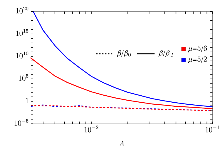
Figure 5: Ratio between mass fraction $\beta$ for the non-Gaussian case between the prescriptions presented in this paper and the prescription presented in Ref. [23]. We fix the shape parameter $q=0.5$ (as a consequence also the threshold using Eq. (2.11)) and the shape of power spectrum $\Delta=1$ while we vary the amplitude.

6 Conclusions and some further final considerations

In this paper we have shown that the abundance of PBHs is dominated by the broadest profiles of the compaction function, even though they are not the typical ones, unless the power spectrum of the curvature perturbation is very peaked. The corresponding threshold is therefore always 2/5. We have also discussed how this result makes the tension between overproducing PBHs and fitting the recent PTA data on gravitational waves even worse than recent analysis.

On more general grounds, given the dependence of the critical threshold on the profile of the compaction function, the natural question is if it possible to construct an observable whose critical threshold does not depend at all on the profiles of the peaks. In Ref. [6] it has been proven numerically that the volume average of the compaction function, calculated in a volume of sphere of radius $R_{m}$

$$\overline{C}(R_{m})=\frac{3}{R_{m}^{3}}\int_{0}^{R_{m}}{\rm d}x\,x^{2}\,C(x)$$ (6.1)

has a critical threshold equal to 2/5 independently from the profile. In the case of a broad compaction function, whose critical threshold is 2/5, and since $\overline{C}(R_{m})\simeq C(R_{m})$, it is trivial that the volume average has the same critical value 2/5. The case of a very spiky compaction function corresponds to a flat universe with in it a sphere of radius $R_{m}$ and constant curvature $K(R)=C(R)/R^{2}$, that is $C(R)$ scales like $R^{2}$. One then obtains

$$\overline{C}(R_{m})=3\frac{C(R_{m})}{R_{m}^{5}}\int_{0}^{R_{m}}{\rm d}x\,x^{4}=\frac{3}{5}C(R_{m})=\frac{3}{5}\cdot\frac{2}{3}=\frac{2}{5},$$ (6.2)

where it is used that for very spiky compaction functions the critical value is 2/3.

Assuming a universal threshold, one can then write the probability that the volume average compaction function is larger than 2/5 even for the non-Gaussian case as (we use here threshold statistics to make the point, one could similarly use peak theory)

$$P\left[\overline{C}(R_{m})>2/5\right] = \Big{<}\Theta_{H}\left[\overline{C}(R_{m})-2/5\right]\Big{>}$$ (6.3)

$$= \frac{1}{2\pi}\int\left[DC(r)\right]P\left[C(r)\right]\int_{2/5}^{\infty}{\rm d}\alpha\int_{-\infty}^{\infty}{\rm d}\phi\,e^{i\phi(\overline{C}(R_{m})-\alpha)}$$

which can be written as

$$P\left[\overline{C}(R_{m})>2/5\right]=\int_{2/5}^{\infty}{\rm d}\alpha\int_{-\infty}^{\infty}{\rm d}\phi\,e^{-i\phi\alpha}\cdot Z[J],$$ (6.4)

with

$$Z[J]=\int\left[DC({\bf x})\right]P\left[C({\bf x})\right]e^{i\int{\rm d}^{3}x\,J({\bf x})C({\bf x})},\quad J({\bf x})=\,V^{-1}_{R_{m}}\,\phi\,\Theta_{H}(\overline{r}_{m}-r)\,,$$ (6.5)

and the measure $\left[DC(r)\right]$ is such that

$$\int\left[DC({\bf x})\right]P\left[C({\bf x})\right]=\int\left[DC(r)\right]P\left[C(r)\right]=1.$$ (6.6)

The correlators are determined by the expansion of the partition function $Z[J]$ in terms of the source $J$, while the corresponding expansion of $W[J]=\ln Z[J]$ generates the connected correlation functions. We will denote the latter as

$$\xi^{(n)}({\bf x}_{1},\cdots,{\bf x}_{n})=\frac{\delta}{\delta J({\bf y}_{1})}\cdots\frac{\delta}{\delta J({\bf y}_{n})}\ln Z[J],$$ (6.7)

and the connected cumulants of the volume average linear compaction function as

$$\langle\overline{C}^{n}(R_{m})\rangle = \frac{1}{V^{n}_{R_{m}}}\int{\rm d}^{3}x_{1}\cdots{\rm d}^{3}x_{n}\prod_{i=1}^{n}\xi^{(n)}({\bf x}_{1},\cdots,{\bf x}_{n})\,\Theta_{H}(R_{m}-x_{i})$$

$$= \prod_{i=1}^{n}\int\frac{{\rm d}^{3}k_{i}}{(2\pi)^{3}}P_{N}({\bf k}_{1},\cdots,{\bf k}_{n})W(k_{1}R_{m})\cdots W(k_{n}R_{m})\,\delta_{D}^{(n)}({\bf k}_{1}+\cdots+{\bf k}_{n}),$$

$$\langle C_{\zeta}({\bf k}_{1}),\cdots,C_{\zeta}({\bf k}_{n})\rangle = P_{N}({\bf k}_{1},\cdots,{\bf k}_{n})\delta_{D}^{(n)}({\bf k}_{1}+\cdots+{\bf k}_{n}).$$ (6.8)

Then, we may write

$$\ln Z[J] = \sum_{n=2}^{\infty}\frac{(-1)^{n}}{n!}\int{\rm d}^{3}{\bf y}_{1}\cdots\int{\rm d}^{3}{\bf y}_{n}\,J_{i_{1}}({\bf y}_{1})\cdots J_{i_{n}}({\bf y}_{n})\xi^{(n)}({\bf x}_{i_{1}},\cdots,{\bf x}_{i_{n}})$$ (6.9)

$$= \sum_{n=2}^{\infty}\frac{(-1)^{n}}{n!}\phi^{n}\langle\overline{C}^{n}\rangle.$$

Using the above expression for the connected partition function, we find that the one-point statistics of Eq. (6.3) can be written as

$$P\left[\overline{C}(R_{m})>2/5\right]= (2\pi)^{-1/2}\int_{2/5}^{\infty}{\rm d}a\,\exp\left\{\sum_{n=3}^{\infty}\frac{(-1)^{n}}{n!}\langle\overline{C}^{n}\rangle\frac{\partial^{n}}{\partial a^{n}}\right\}\exp{\left(-\frac{a^{2}}{2\sigma_{\overline{C}}^{2}}\right)}$$ (6.10)

$$= (2\pi)^{-1/2}\int_{2/5}^{\infty}{\rm d}a\,\left(1-\frac{1}{3!}\langle\overline{C}_{\zeta}^{3}\rangle\frac{{\rm d}^{3}}{{\rm d}a^{3}}+\frac{1}{4!}\langle\overline{C}^{4}\rangle\frac{{\rm d}^{4}}{{\rm d}a^{4}}+\cdots\right)\exp{\left(-\frac{a^{2}}{2\sigma_{\overline{C}}^{2}}\right)}$$

$$= h_{0}(2/5)+\frac{1}{\sqrt{2\pi}}\sum_{n\geq 3}\frac{1}{2^{\frac{n}{2}}n!}\frac{c_{n}}{\sigma_{\overline{C}}^{n-1}}e^{-4/50\sigma_{\overline{C}}^{2}}H_{n-1}\left(\frac{2/5}{\sqrt{2}\sigma_{\overline{C}}}\right),$$

where

$$h_{0}(2/5)=\frac{1}{2}{\rm Erfc}\left(\frac{1}{\sqrt{2}}\frac{2/5}{\sigma_{\overline{C}}}\right),$$ (6.11)

$\sigma_{\overline{C}}$ is the variance, $H_{n}$ are Hermite polynomials and we have defined in Eq. (6.10) the parameters $c_{n}$ as

$$c_{n}=\sum_{\hat{p}[n]}\,\,\,\,\prod_{\begin{subarray}{c}p_{1}m_{1}+\cdots p_{r}m_{r}=n\\ p_{i}\geq 0,m_{i}\geq 3\end{subarray}}\frac{n!}{m_{1}!\cdots m_{r}!\,p_{1}!\cdots p_{r}!}\,\langle\overline{C}^{m_{1}}\rangle^{p_{1}}\cdots\langle\overline{C}^{m_{r}}\rangle^{p_{r}},$$ (6.12)

where $\hat{p}[n]$ denotes the partitions of the integer $n$ into numbers $m_{i}\geq 3$.

Given the statistics of the curvature perturbation, one can calculate the abundance of PBHs using the volume average of the linear compaction function, relying solely on superhorizon quantities. Generally, determining the statistics of the curvature perturbation can be challenging and computing the connected cumulants is highly non-trivial. We left this task for future investigation.

Acknowledgements

We thank V. De Luca and G. Franciolini for useful comments on the draft. A.I. and A.R. acknowledge support from the Swiss National Science Foundation (project number CRSII5_213497). A.K. is supported by the PEVE-2020 NTUA programme for basic research with project number 65228100. D. P. and A.R. are supported by the Boninchi Foundation for the project “PBHs in the Era of GW Astronomy”.

References

- [1] E. Bagui et al. [LISA Cosmology Working Group], [astro-ph.CO/2310.19857].
- [2] G. Franciolini, V. Baibhav, V. De Luca, K. K. Y. Ng, K. W. K. Wong, E. Berti, P. Pani, A. Riotto and S. Vitale, Phys. Rev. D 105 (2022) no.8, 083526 [gr-qc/2105.03349].
- [3] V. De Luca, A. Kehagias and A. Riotto, Phys. Rev. D 108 (2023) no.6, 063531 [astro-ph.CO/2307.13633].
- [4] G. Franciolini, A. Ianniccari, A. Kehagias, D. Perrone and A. Riotto, [astro-ph.CO/2311.03239].
- [5] T. Harada, C. M. Yoo and Y. Koga, Phys. Rev. D 108 (2023) no.4, 043515 [gr-qc/2304.13284].
- [6] A. Escrivà, C. Germani and R. K. Sheth, Phys. Rev. D 101 (2020) no.4, 044022 [gr-qc/1907.13311].
- [7] I. Musco, Phys. Rev. D 100 (2019) no.12, 123524 [gr-qc/1809.02127].
- [8] I. Musco, V. De Luca, G. Franciolini and A. Riotto, Phys. Rev. D 103 (2021) no.6, 063538 [astro-ph.CO/2011.03014].
- [9] Y. Hoffman and J. Shaham, Astrophys. J. 297 (1985), 16-22.
- [10] Y. F. Cai, X. Chen, M. H. Namjoo, M. Sasaki, D. G. Wang and Z. Wang, JCAP 05 (2018), 012 [astro-ph.CO/1712.09998].
- [11] M. Kawasaki, N. Kitajima and T. T. Yanagida, Phys. Rev. D 87, no.6, 063519 (2013) [hep-ph/1207.2550].
- [12] M. Sasaki, J. Valiviita and D. Wands, Phys. Rev. D 74 (2006), 103003 [astro-ph/0607627].
- [13] G. Ferrante, G. Franciolini, A. Iovino, Junior. and A. Urbano, JCAP 06 (2023), 057 [astro-ph.CO/2305.13382].
- [14] M. W. Choptuik, Phys. Rev. Lett. 70 (1993), 9-12 [PhysRevLett.70.9].
- [15] C. R. Evans, J. S. Coleman, Phys. Rev. Lett. 72 (1994), 1782-1785 [gr-qc/9402041].
- [16] I. Musco, J. C. Miller Classical and Quantum Gravity, 30 (2013) no.14, 145009 [astro-ph.CO/1201.2379].
- [17] M. Sasaki, T. Suyama, T. Tanaka and S. Yokoyama, Classical and Quantum Gravity, 35 (2018) no.6, 063001 [astro-ph.CO/1801.05235].
- [18] M. Biagetti, G. Franciolini, A. Kehagias and A. Riotto, JCAP 07 (2018), 032 [astro-ph.CO/1804.07124].
- [19] M. Biagetti, V. De Luca, G. Franciolini, A. Kehagias and A. Riotto, Phys. Lett. B 820 (2021), 136602 [astro-ph.CO/2105.07810].
- [20] E. Tomberg, Phys. Rev. D 108 (2023) no.4, 4 [astro-ph.CO/2304.10903].
- [21] A. Escrivà, V. Atal and J. Garriga, JCAP 10 (2023), 035 [astro-ph.CO/2306.09990].
- [22] K. Uehara, A. Escrivà, T. Harada, D. Saito and C. M. Yoo, [gr-qc/2401.06329].
- [23] G. Ferrante, G. Franciolini, A. Iovino, Junior. and A. Urbano, Phys. Rev. D 107, no.4, 043520 (2023) [astro-ph.CO/2211.01728].
- [24] A. D. Gow, H. Assadullahi, J. H. P. Jackson, K. Koyama, V. Vennin and D. Wands, EPL 142 (2023) no.4, 49001 [astro-ph.CO/2211.08348].
- [25] S. Young, JCAP 05 (2022) no.05, 037 [astro-ph.CO/2201.13345].
- [26] G. Franciolini, A. Iovino, Junior., V. Vaskonen and H. Veermae, Phys. Rev. Lett. 131 (2023) no.20, 201401 [astro-ph.CO/2306.17149].
- [27] G. Domènech, Universe 7 (2021) no.11, 398 [gr-qc/2109.01398].
- [28] G. Agazie et al. [NANOGrav], Astrophys. J. Lett. 951 (2023) no.1, L8 [astro-ph.HE./2306.16213]
- [29] A. Escrivà, Y. Tada, S. Yokoyama and C. M. Yoo, JCAP 05, no.05, 012 (2022) [astro-ph.CO/2202.01028].
- [30] H. Firouzjahi and A. Riotto, Phys. Rev. D 108, no.12, 123504 (2023) [astro-ph.CO/2309.10536].
- [31] T. Harada, C. M. Yoo and K. Kohri, Phys. Rev. D 88, no.8, 084051 (2013) [erratum: Phys. Rev. D 89, no.2, 029903 (2014)] [astro-ph.CO/1309.4201].