Proximal Causal Inference for Conditional Separable Effects

Abstract

Scientists often pose questions about treatment effects on outcomes conditional on a post-treatment event. However, defining, identifying, and estimating causal effects conditional on post-treatment events requires care, even in perfectly executed randomized experiments. Recently, the conditional separable effect (CSE) was proposed as an interventionist estimand, corresponding to scientifically meaningful questions in these settings. However, while being a single-world estimand, which can be queried experimentally, existing identification results for the CSE require no unmeasured confounding between the outcome and post-treatment event. This assumption can be violated in many applications. In this work, we address this concern by developing new identification and estimation results for the CSE in the presence of unmeasured confounding. We establish nonparametric identification of the CSE in both observational and experimental settings when certain proxy variables are available for hidden common causes of the post-treatment event and outcome. We characterize the efficient influence function for the CSE under a semiparametric model of the observed data law in which nuisance functions are a priori unrestricted. Moreover, we develop a consistent, asymptotically linear, and locally semiparametric efficient estimator of the CSE using modern machine learning theory. We illustrate our framework with simulation studies and a real-world cancer therapy trial.

Keywords: confounding bridge function, controlled direct effect, mixed-bias property, principal stratum effect, truncation by death

1 Introduction

In many observational studies and randomized trials, outcomes of interest are defined conditional on a post-treatment event. For example, Ding et al. (2011), Wang et al. (2017), Yang and Ding (2018), and Stensrud et al. (2022a) analyzed the Southwest Oncology Group (SWOG) Trial, where male refractory prostate cancer patients were assigned to one of two chemotherapies. Their objective was to estimate the causal effect of cancer chemotherapies on quality of life in a subsequent follow-up period. Quality of life can only be assessed for patients who have survived until the follow-up period, and the causal effect of interest is only relevant to survivors. As another example, Jemiai et al. (2007) analyzed an HIV vaccine trial to study the effect of HIV vaccines on viral load. Here, the viral load of uninfected individuals is well-defined as zero, meaning that the causal effect among uninfected individuals is also zero. Yet, their scientific question of interest was formulated around causal effects on “an outcome measured after a post-randomization event occurs.”

Several causal estimands can be considered in the presence of post-treatment events. Robins and Greenland (1992) defined a controlled direct effect, which is the effect of treatment on the outcome in a hypothetical scenario where a particular post-treatment event cannot occur. Frangakis and Rubin (2002) introduced a so-called principal stratum effect, which is a causal effect in the subset of individuals who would experience a meaningful post-treatment event status regardless of the treatment they received. We refer to Robins (1986) for an earlier definition of this type of effect in the context of truncation by death. In the SWOG trial, the controlled direct effect is defined as the effect of cancer treatment on quality of life had, contrary to fact, every patient been kept alive via an external intervention. A particular principal stratum effect is defined as the effect of cancer treatment on quality of life among “always survivors,” that is, patients who would survive regardless of the cancer treatments they received; this principal stratum effect is also referred to as the survivor average causal effect. Analogously, in the HIV vaccine trial, the controlled direct effect is the effect of an HIV vaccine on viral load had every individual been infected, and the key principal stratum effect of interest is the effect of an HIV vaccine on viral load among “always-infected individuals,” that is, individuals who would be infected regardless of HIV vaccination status.

However, these causal estimands have some limitations. First, the controlled direct effect is defined under an intervention where everyone experiences a post-treatment event, which may be unrealistic and infeasible. For example, it is unclear whether assessing the causal effect of cancer therapy on quality of life in a hypothetical scenario where everyone is somehow made to survive is of subject-matter interest. Second, although the principal stratum effect has been advocated in various settings (Rubin, 2006; VanderWeele, 2011; Ding and Lu, 2016), this effect is defined in a particular subgroup that cannot be identified from real-world data without strong assumptions. Moreover, this subgroup may represent an atypical (possibly non-existent) subset of the population, limiting its practical utility. For more in-depth discussion on this topic, we refer readers to Robins (1986), Robins et al. (2007), Joffe (2011), Robins and Richardson (2011), Dawid and Didelez (2012), Robins et al. (2022), and Stensrud et al. (2022a).

Instead of considering principal causal effects, Stensrud et al. (2022a) proposed the conditional separable effect (CSE), which is applicable when the primary outcome is only of interest conditional on a post-treatment event. The definition of the CSE is inspired by the seminal treatment composition idea of Robins and Richardson (2011). When considering the CSE in this paper, we will require that the treatment in the current study can be conceived as a composite of two components, say $A_{Y}$- and $A_{D}$-components, where the $A_{Y}$-component directly affects the outcome but does not affect the post-treatment event and the $A_{D}$-component directly affects the post-treatment event but does not directly affect the outcome. The CSE is then defined as the causal effect of the $A_{Y}$-component on the outcome within a subgroup of the population experiencing a post-treatment event, provided that the $A_{D}$-component is set at a certain level. This implies that the CSE can be interpreted as the direct effect of treatment on the outcome through the $A_{Y}$-component in a specific subgroup of the population. Unlike the principal stratum effects, the two key conditions can in principle be falsified in future experiments. In other words, unlike the subgroup used to define the principal stratum effects, such as always survivors and always-infected individuals, the subgroup used to define the CSE is potentially experimentally observable. Unlike the controlled direct effect, the CSE does not require conceiving of hypothetical interventions on the post-treatment event.

For identification and estimation of the CSE, Stensrud et al. (2022a) relied on the assumption that there is no unmeasured common cause of the outcome and the post-treatment event. This assumption is often justified by the belief that the measured covariates are rich enough to account for confounding between the outcome and the post-treatment event. However, this assumption is questionable in many real-world applications, as collecting all confounding variables is a daunting task. In the examples mentioned above, unmeasured variables such as medical history, chronic illnesses, lifestyle elements (e.g., smoking, alcohol consumption, physical activity), and sociodemographic status can affect both the outcome and post-treatment event, casting doubt on the no unmeasured confounding assumption, even in randomized experiments.

Several recent papers (Lipsitch et al., 2010; Kuroki and Pearl, 2014; Miao et al., 2018, 2020; Shi et al., 2020a, b; Tchetgen Tchetgen et al., 2020; Kallus et al., 2021; Mastouri et al., 2021; Ghassami et al., 2022; Cui et al., 2023; Dukes et al., 2023; Ying et al., 2023) have focused on mitigating bias due to unmeasured confounding by carefully leveraging proxies for the latter. This constitutes the so-called proximal causal inference framework, which relies on the key assumption that one has access to two types of proxies: (i) treatment-confounding proxies, which may or may not be causally related to the treatment of interest, and are related to the outcome only through an association with unmeasured confounders of the treatment and the outcome; (ii) outcome-confounding proxies, which are potential causes of the outcome and are related an association with to the treatment only through unmeasured confounders. Using treatment- and outcome-confounding proxies appropriately, one can potentially identify and estimate causal effects. Miao et al. (2018) established sufficient conditions for nonparametric identification of the average treatment effect in the point treatment setting. Building upon this work, Tchetgen Tchetgen et al. (2020) extended the result to time-varying treatments using so-called proximal g-computation, a generalization of Robins’ g-computation algorithm (Robins, 1986). Cui et al. (2023) provided alternative identification conditions for proximal causal inference and developed a doubly robust semiparametric locally efficient estimator of the average treatment effect using proxies. Kallus et al. (2021), Mastouri et al. (2021), and Ghassami et al. (2022) discussed estimation of the average treatment effect using nonparametric methods. Lastly, Dukes et al. (2023) studied semiparametric proximal causal inference in mediation settings, focusing on identification and semiparametric estimation of natural direct and indirect effects.

The current paper focuses on identification and estimation of the CSE in both observational and experimental settings, allowing for the possibility of hidden confounding factors. Therefore, the paper complements Stensrud et al. (2022a), which a priori ruled out the presence of such confounding. In addition, existing approaches in the proximal causal inference framework are not readily applicable for inferring the CSE because the CSE is defined conditional on a post-treatment event, a situation prior proximal causal inference methods do not address. Here, we extend the proximal causal inference framework and establish formal identification of the CSE by introducing new forms of so-called confounding bridge functions (Miao et al., 2020) that capture the potential impact of hidden common causes of the outcome and post-treatment events, by carefully incorporating treatment and outcome proxy factors. In addition, we characterize the efficient influence function for the CSE under a semiparametric model of the observed data law which allows confounding bridge functions to be a priori unrestricted. We develop a semiparametric locally efficient estimator that is consistent and asymptotically normal for the CSE. Notably, the proposed estimator employs recent machine learning theory to estimate data-adaptively nuisance components without the need for specifying restrictive parametric models.

In Section 2, we describe the general setup, introduce notation, and state key assumptions. We establish nonparametric identification of the CSE in observational settings in Section 3. In Section 4, we develop a semiparametric estimator of the CSE. We present the results for experimental settings in Section A.11 of the Supplementary Material. We perform simulation studies to assess the finite-sample performance of the proposed estimator in Section 5. In Section 6, we then apply the proposed method to a real-world randomized trial to evaluate the effect of cancer chemotherapies on quality of life improvements among prostate cancer patients. We end the paper with concluding remarks in Section 7. Additional discussions and proofs of the results are relegated to the Supplementary Material.

2 Setup and Assumptions

2.1 Setup

Let $N$ be the number of study units in the data, indexed by the subscript $i=1,\ldots,N$. We will suppress the subscript unless necessary. For each study unit, we observe independent and identically distributed (i.i.d.) data $O=(Y,D,A,L)$; here, $Y$ is the outcome of interest and $D\in\{0,1\}$ is a binary post-treatment event which occurs prior to $Y$ can occur. Without loss of generality, we encode $D=0$ to indicate that a unit experiences the post-treatment event for which $Y$ becomes relevant. Next, $A\in\{0,1\}$ denotes the treatment status where $A=0$ and $A=1$ indicate that a study unit is assigned to the control and treatment arms in the current two-arm study, respectively. The vector $L$ consists of observed baseline covariates. In the SWOG trial, $Y$ is defined as change in quality of life between baseline and one-year follow-up, $D$ is the indicator of whether a patient died during the study period (i.e., truncation by death), $A$ encodes the cancer therapy assigned to a patient, and $L$ consists of pre-treatment covariates such as age and race. Clearly, quality of life at follow up is only relevant, and in fact only well-defined for a person who is alive at follow-up; see Section 6 for details on these variables.

Throughout the paper, we suppose that the binary treatment can reasonably be conceptualized as a composition of two binary components, say $A_{Y}\in\{0,1\}$ and $A_{D}\in\{0,1\}$. Specifically, $A_{Y}$- and $A_{D}$-components are defined as modified treatment, which, e.g., could be components of $A$, that only directly affect the outcome $Y$ and the post-treatment event $D$, respectively; see Assumption (A4) and related discussions for details. In particular, this decomposition is valid when the treatment in the current study comprises two physically distinct components. In the SWOG trial, each cancer therapy consisted of two drugs: a pain reliever and an inhibitor of cancer cell proliferation, which can be reasonably seen as $A_{Y}$- and $A_{D}$-components, respectively; see Section 6 for more discussions.

More generally, it is not required for one to be able to physically decompose the original treatment. Rather, we require the conceptualization of modified treatments $A_{Y}$ and $A_{D}$ that, when set to the same value $a$, leads to exactly the same values of $Y$ and $D$ as assigning $A$ to $a$ (Stensrud et al., 2022b, Section 5). To illustrate this point, we revisit an example from Stensrud et al. (2022b). Suppose that the goal is to evaluate the effect of diethylstilbestrol (DES) on prostate cancer mortality among survivors who did not succumb to other causes. DES, an estrogen agent, appears to reduce prostate cancer mortality by suppressing testosterone production while simultaneously increasing cardiovascular mortality through an estrogen-induced synthesis of coagulation factors (Turo et al., 2014). Given the distinct causal mechanisms through which DES affects prostate cancer mortality and mortality from other causes, we could conceptualize a new treatment that, like DES, stops testosterone production but, unlike DES, has no other effect on the cardiovascular system. Indeed, such treatment, e.g., luteinizing hormone-releasing hormone agonists, is now given to treat individuals with prostate cancer. Motivated by examples presented in Pearl (2001), Robins and Richardson (2011) also discussed a plausible treatment decomposition in a mediation context, using nicotine and non-nicotine components in cigarettes.

In the current two-arm study, the treatment $A$ and its $A_{Y}$- and $A_{D}$-components satisfy a deterministic relationship. Specifically, $A$ is defined as a specific combination of $(A_{Y},A_{D})$ in the sense that $A=a$ if and only if $A_{Y}=A_{D}=a$ for $a=0,1$. On the other hand, consider a four-arm trial that can potentially be conducted in the future, in which each study unit is assigned to one of the following four treatment levels $(A_{Y},A_{D})\in\{(0,0),(1,0),(0,1),(1,1)\}$. An analogous hypothetical trial has been considered in the context of mediation (Robins and Richardson, 2011; Robins et al., 2022) and competing risk (Stensrud et al., 2021), and the CSE (Stensrud et al., 2022a). Therefore, the two treatment arms $(A_{Y},A_{D})\in\{(1,0),(0,1)\}$ are not assigned in the two-arm study.

Let $D^{(a_{Y},a_{D})}\in\{0,1\}$ and $Y^{(a_{Y},a_{D})}\in\mathbbm{R}$ be the potential post-treatment event and the potential outcome, respectively, had $(A_{Y},A_{D})$ been assigned to $(a_{Y},a_{D})\in\{(0,0),(1,0),\\ (0,1),(1,1)\}$ in the four-arm trial. The potential post-treatment event and the potential outcome in the two-arm study reduce to $D^{(a)}=D^{(a_{Y}=a,a_{D}=a)}$ and $Y^{(a)}=Y^{(a_{Y}=a,a_{D}=a)}$ for $a=0,1$. In addition, following the notation in Stensrud et al. (2022a), let $G$ be the potential future four-arm trial, and let $V(G)$ be a node represented on the causal directed acyclic graph (DAG) (Pearl, 2009). For example, we use $Y(G)$, $D(G)$, $A_{Y}(G)$, and $A_{D}(G)$ to denote the outcome, post-treatment event, and two treatment components that would be observed in the four-arm trial.

Throughout the paper, we allow for the possibility of hidden confounding factors, denoted by $U$, which are common causes of $(Y,D,A)$. Based on the relationship with $U$, we assume that the measured covariate $L$ can be partitioned into three variables $(W,Z,X)$, which are distinguished as follows. First, $W$ and $Z$ are outcome- and treatment-confounding proxies, respectively; see Assumption (A6) for formal conditions that $W$ and $Z$ must satisfy as valid outcome and treatment-confounding proxies. Second, $X$ is a collection of measured baseline confounders that may causally impact $(Y,D,A)$. We formalize the relationships between these variables in the next section.

Lastly, we introduce additional notation used throughout. An abbreviation “a.s.” stands for “almost surely.” Let $\mathcal{L}_{2}(V)=\{f(V)\,\big{|}\,E\{f^{2}(V)\}<\infty\}$ be a Hilbert space of functions of a random variable $V$ with finite variance equipped with the inner product $\langle f_{1},f_{2}\rangle=E\{f_{1}(V)f_{2}(V)\}$. For a sequence of random variables $\{V_{N}\}$ and a sequence of numbers $\{r_{N}\}$, let $V_{N}=O_{P}(r_{N})$ and $V_{N}=o_{P}(r_{N})$ denote that $V_{N}/r_{N}$ is stochastically bounded and converges to zero in probability as $N\rightarrow\infty$, respectively. Let $V_{N}\stackrel{{\scriptstyle D}}{{\rightarrow}}V$ mean that $V_{N}$ weakly converges to a random variable $V$ as $N\rightarrow\infty$.

2.2 Assumptions

We begin by introducing key assumptions.

• (Consistency) $Y=Y^{(a=A)}$ and $D=D^{(a=A)}$ a.s.

• (Latent Ignorability) For $a=0,1$, $(Y^{(a)},D^{(a)})\rotatebox[origin={c}]{90.0}{$\models$}A\,\big{|}\,(X,U)$.

• (Latent Positivity) For $a=0,1$, (i) $\Pr(D=0\,\big{|}\,A=a,X,U)>0$ a.s. and (ii) $\Pr(A=a\,\big{|}\,X,U)>0$ a.s.

Assumptions (A1)-(A3) are standard consistency, ignorability, and positivity. Note that (A2) and (A3) are fairly mild conditions as $U$ need not be observed; importantly, we note that while (A2) conditions on $U$, we do not make the corresponding assumption conditional on $X$ only, i.e., we generally allow for $(Y^{(a)},D^{(a)})$ not independent of $A$ given $X$. This is a critical difference between the current setting and that considered by Stensrud et al. (2022a), which makes the more restrictive assumption that $(Y^{(a)},D^{(a)})$ independent of $A$ given $X$. In addition, (A2) allows for unmeasured confounding of $D$ and $Y$. This condition is less restrictive than the so-called principal ignorability condition (Jo and Stuart, 2009; Ding and Lu, 2016; Feller et al., 2017; Forastiere et al., 2018), which posits the absence of unmeasured confounding between $D$ and $Y$. In experimental settings, $A$ is unconfounded by virtue of randomization; see Section A.11 for details on our approach in this case.

Next, following Stensrud et al. (2022a) and Stensrud et al. (2022b), we formalize the required conditions for the $A_{Y}$- and $A_{D}$-components in a hypothetical four-arm trial $G$:

• ($A_{D}$-Partial Isolation) For $a_{Y}=0,1$, $Y^{(a_{Y},a_{D}=1)}(G)=Y^{(a_{Y},a_{D}=0)}(G)$ if $D^{(a_{Y},a_{D}=1)}(G)=D^{(a_{Y},a_{D}=0)}(G)=0$;

• ($A_{Y}$-Partial Isolation) For $a_{D}=0,1$, $D^{(a_{Y}=1,a_{D})}(G)=D^{(a_{Y}=0,a_{D})}(G)$.

Assumption (A4)-(i) states that, in a hypothetical future four-arm trial $G$, a unit’s outcome would not be causally affected by the $A_{D}$-component provided that the unit experiences the post-treatment event. Likewise, Assumption (A4)-(ii) states that the post-treatment event would not be causally affected by the $A_{Y}$-component. Assumption (A4) could be in principle falsified from a future four-arm trial $G$ in which $A_{Y}$ and $A_{D}$ are randomized.

As discussed in Section 1, we focus on the CSE as the estimand of interest, which is formally defined as

$$\tau_{\text{CSE}}^{*}(a_{D})=\psi^{*}(1,a_{D})-\psi^{*}(0,a_{D})\ ,\ \psi^{*}(a_{Y},a_{D})=E\big{\{}Y^{(a_{Y},a_{D})}\,\big{|}\,D^{(a_{Y},a_{D})}=0\big{\}}\ .$$ (1)

Under (A4)-(ii) (i.e., $A_{Y}$-partial isolation), the CSE reduces to $\tau_{\text{CSE}}^{*}(a_{D})=E\big{\{}Y^{(a_{Y}=1,a_{D})}-Y^{(a_{Y}=0,a_{D})}\,\big{|}\,D^{(a_{D})}=0\big{\}}$, which is interpreted as the average causal effect of $A_{Y}$ on $Y$ when the other treatment component is assigned as $A_{D}=a_{D}$ among the subset of study units who do not experience the post-treatment event under $A_{D}=a_{D}$. In the SWOG trial, the CSE can be viewed as the average causal effect of pain relievers on the change in quality of life among patients who would survive had they received a specific cancer cell proliferation inhibitor; see Section 6 for details. Without (A4)-(i) (i.e., $A_{D}$-partial isolation), there can be causal paths from $A$ to $Y$ that are not intersected by $D$, such as a path $A_{D}\rightarrow W\rightarrow Y$, indicating that $\tau_{\text{CSE}}^{*}(a_{D})$ only captures the direct effect, but not all effects of $A$ on $Y$ relative to the post-treatment event. On the other hand, under (A4)-(i) and (A4)-(ii), (i.e., full isolation), all causal paths from $A_{D}$ to $Y$ are intersected by $D$, and all causal paths from $A_{Y}$ to $Y$ are not intersected by $D$, implying that the CSE can be viewed as all effects of $A$ on $Y$ not intersected by $D$.

In order to establish identification of $\psi^{*}(a_{Y},a_{D})$, we make the following latent dismissible condition.

• (Latent Dismissible Condition) (i) $Y(G)\rotatebox[origin={c}]{90.0}{$\models$}A_{D}(G)\,\big{|}\,(A_{Y}(G),D(G)=0,X(G),U(G))$ and (ii) $D(G)\rotatebox[origin={c}]{90.0}{$\models$}A_{Y}(G)\,\big{|}\,(A_{D}(G),X(G),U(G))$.

Assumption (A5)-(i) states that, in a hypothetical future four-arm trial $G$, the outcome would be independent of the $A_{D}$-component conditional on $(A_{Y},X,U)$ among units experiencing the post-treatment event. Likewise, Assumption (A5)-(ii) states that the post-treatment event would be independent of the $A_{Y}$-component conditional on $(A_{D},X,U)$. Assumption (A5) can be interpreted as conditions on causal mechanisms between $(A_{Y},A_{D})$ and $(Y,D)$. Specifically, suppose that a causal DAG for variables $(A_{Y}(G),A_{D}(G),Y(G),\\ D(G),U(G))$ represents a Finest Fully Randomized Causally Interpreted Structural Tree Graph (FFRCISTG) model (Robins, 1986; Richardson and Robins, 2013) under $G$ where lack of arrows on this causal DAG encodes the assumption that an individual-level causal effect is absent for every individual in the study population. Then, as established by Stensrud et al. (2022a), Assumption (A5) implies Assumption (A4).

Under Assumptions (A1)-(A5), $\psi^{*}(a_{Y},a_{D})$ can be written as $\psi^{*}(a_{Y},a_{D})=\psi_{N}^{*}(a_{Y},a_{D})/\psi_{D}^{*}(a_{D})$ where

$$\begin{array}[]{l}\psi_{N}^{*}(a_{Y},a_{D})=E\big{\{}E\big{(}Y\,\big{|}\,A=a_{Y},D=0,X,U\big{)}\Pr\big{(}D=0\,\big{|}\,A=a_{D},X,U\big{)}\big{\}}\ ,\\ \psi_{D}^{*}(a_{D})=E\big{\{}\Pr\big{(}D=0\,\big{|}\,A=a_{D},X,U\big{)}\big{\}}\ .\end{array}$$ (4)

See Section A.2 of the Supplementary Material for details reproducing Theorem 1 of Stensrud et al. (2022a). However, (4) cannot serve as an identification formula as $U$ is unmeasured. In order to establish identification, one can use a treatment-confounding proxy $Z$ and an outcome-confounding proxy $W$, which are formally defined as follows:

• (Proxies) For $a=0,1$, (i) $Z\rotatebox[origin={c}]{90.0}{$\models$}Y^{(a)}\,\big{|}\,(A,D^{(a)},X,U)$; (ii) $Z\rotatebox[origin={c}]{90.0}{$\models$}D^{(a)}\,\big{|}\,(A,X,U)$; (iii) $W\rotatebox[origin={c}]{90.0}{$\models$}D^{(a)}\,\big{|}\,(X,U)$; (iv) $W\rotatebox[origin={c}]{90.0}{$\models$}(A,Z)\,\big{|}\,(D^{(a)},X,U)$.

Assumption (A6) states that, conditional on $(X,U)$, $Z$ does not have a causal effect on $Y$ and $D$, and $(A,D)$ do not causally impact $W$. Additionally, $W$ and $Z$ are associated with each other to the extent that they are associated with $U$. These conditions extend analogous proxy conditions in Miao et al. (2018); Tchetgen Tchetgen et al. (2020); Dukes et al. (2023) to the current setting. Figure 1 illustrates a single world intervention graph (SWIG; Richardson and Robins, 2013) compatible with Assumptions (A4)-(A6).

Figure 1: Single World Intervention Graphs (SWIG) compatible with Assumptions (A4)-(A6).

For identification, we also require certain completeness conditions:

• (Completeness) Let $g(U)$ be an arbitrary square-integrable function. We have:

  • $E\big{\{}g(U)\,\big{|}\,Z,A=a_{D},D=0,X\big{\}}=0$ for all $(Z,X)$ a.s. implies $g(U)=0$ a.s.;

  • $E\big{\{}g(U)\,\big{|}\,Z,A=a_{Y},X\big{\}}=0$ for all $(Z,X)$ a.s. implies $g(U)=0$ a.s.;

  • $E\big{\{}g(U)\,\big{|}\,W,A=a_{D},D=0,X\big{\}}=0$ for all $(W,X)$ a.s. implies $g(U)=0$ a.s.;

  • $E\big{\{}g(U)\,\big{|}\,W,A=a_{Y},X\big{\}}=0$ for all $(W,X)$ a.s. implies $g(U)=0$ a.s..

Completeness has been routinely used for identification in the context of nonparametric instrumental variable regression (Newey and Powell, 2003), measurement error model (Hu and Schennach, 2008), longitudinal data (Freyberger, 2017), nonadditive, endogenous models (Chen et al., 2014), and proximal causal inference (Tchetgen Tchetgen et al., 2020). In words, (A7)-(i) and (ii) imply that any variation in $U$ is associated with some variation in $Z$ conditional on $(A=a_{D},D=0,X)$ and $(A=a_{Y},X)$, respectively; (A7)-(iii) and (iv) are interpreted in a similar manner. Therefore, (A7) implies that proxy variables $Z$ and $W$ vary sufficiently relative to the variability in $U$. To help understand this, suppose that $Z$, $W$, and, $U$ are categorical variables with number of categories $d_{Z}$, $d_{W}$, and $d_{U}$, respectively. Assumption (A7) then can be seen as rank conditions on $(Z,X,U)$ and requires $d_{Z}\geq d_{U}$ and $d_{W}\geq d_{U}$, i.e., $Z$ and $W$ must have at least as many categories as $U$. Of note, (A7)-(i) and (ii) are required to establish identification using outcome confounding bridge functions, and (A7)-(iii) and (iv) are required to establish identification using treatment confounding bridge functions; see Theorems 3.1 for details.

3 Nonparametric Proximal Identification

In this Section, we establish nonparametric identification of the CSE in observational settings using certain key confounding bridge functions which we introduce below. We assume that these confounding bridge functions exist; see Section A.3 of the Supplementary Material for sufficient conditions for their existence. To begin, we define outcome confounding bridge functions. Let $h_{0}^{*}$, $h_{1}^{*}$, and $h_{2}^{*}$ be solutions to the following equations:

$$E\big{\{}Y-h_{1}^{*}(W,X;a_{Y})\,\big{|}\,Z,A=a_{Y},D=0,X\big{\}}=0\text{ a.s.}$$ (5)

$$E\big{\{}(1-D)h_{1}^{*}(W,X;a_{Y})-h_{0}^{*}(W,X;a_{Y},a_{D})\,\big{|}\,Z,A=a_{D},X\big{\}}=0\text{ a.s.}$$ (6)

$$E\big{\{}(1-D)-h_{2}^{*}(W,X;a_{D})\,\big{|}\,Z,A=a_{D},X\big{\}}=0\text{ a.s.}$$ (7)

In words, $h_{1}^{*}(W,X;a_{Y})$ can be viewed as a well-calibrated forecast for $Y$ with respect to $Z$ in the sense that the resulting residual $Y-h_{1}^{*}(W,X;a_{Y})$ is mean zero conditional on $(Z,A=a_{Y},D=0,X)$. Likewise, $h_{0}^{*}(W,X;a_{Y},a_{D})$ and $h_{2}^{*}(W,X;a_{D})$ can be viewed as well-calibrated forecasts relative to $Z$ of $(1-D)h_{1}^{*}(W,X;a_{Y})$ and $(1-D)$, respectively, in the sense that the corresponding residuals are mean zero conditional on $(Z,A=a_{D},X)$. Therefore, $h_{0}^{*}$ is indirectly related to $Y$ via the nested relationship between $h_{1}^{*}$ and $h_{0}^{*}$, i.e., equation (6). If $a_{Y}$ is equal to $a_{D}$, $h_{0}^{*}$ can be defined as below without the need to be defined in terms of the nested relationship involving $h_{1}^{*}$:

$$E\big{\{}Y(1-D)-h_{0}^{*}(W,X;a_{D},a_{D})\,\big{|}\,Z,A=a_{D},X\big{\}}\text{ a.s.}$$ (8)

We now define treatment confounding bridge functions. Suppose that there exist functions $q_{0}^{*}$ and $q_{1}^{*}$ satisfying the following equations:

$$E\big{\{}1-\mathbbm{1}(A=a_{D})q_{0}^{*}(Z,X;a_{D})\,\big{|}\,W,X\big{\}}=0\text{ a.s.}$$ (9)

$$E\big{\{}\mathbbm{1}(A=a_{D})q_{0}^{*}(Z,X;a_{D})-\mathbbm{1}(A=a_{Y})q_{1}^{*}(Z,X;a_{Y},a_{D})\,\big{|}\,W,D=0,X\big{\}}=0\text{ a.s.}$$ (10)

An equivalent form for equation (9) is $1/\Pr(A=a_{D}\,\big{|}\,W,X)=E\big{\{}q_{0}^{*}(Z,X;a_{D})\,\big{|}\,W,A=a_{D},X\big{\}}$. Therefore, $q_{0}^{*}(Z,X;a_{D})$ is a well-calibrated forecast relative to $W$ of the inverse probability $1/\Pr(A=a_{D}\,\big{|}\,W,X)$, and the difference between these two functions has mean zero conditional on $(W,A=a_{D},X)$. In case $a_{Y}$ is equal to $a_{D}$, $q_{0}^{*}$ solves (10), implying that $q_{1}^{*}(\cdot;a_{D},a_{D})=q_{0}^{*}(\cdot;a_{D})$. Therefore, $h_{1}^{*}$ and $q_{1}^{*}$ are of substantive interest only if $a_{Y}\neq a_{D}$.

Analogous to other proximal causal inference settings in the literature (Tchetgen Tchetgen et al., 2020; Cui et al., 2023), equations (5)-(10) do not need to admit a unique solution. In fact, any solutions to these equations uniquely identify $\psi^{*}(a_{Y},a_{D})$, as formalized in the following Theorem.

Theorem 3.1.

The following results hold for $(a_{Y},a_{D})\in\{0,1\}^{\otimes 2}$:

• Suppose that Assumptions (A1)-(A6), (A7)-(i), (ii) are satisfied, and that there exist confounding bridge functions $h_{0}^{*}$, $h_{1}^{*}$, and $h_{2}^{*}$ satisfying (5)-(8). Then, we have

  $$\psi_{N}^{*}(a_{Y},a_{D})=E\big{\{}h_{0}^{*}(W,X;a_{Y},a_{D})\big{\}}\ , \psi_{D}^{*}(a_{D})=E\big{\{}h_{2}^{*}(W,X;a_{D})\big{\}}\ .$$

• Suppose that Assumptions (A1)-(A6), (A7)-(i),(iv) are satisfied, and that there exist confounding bridge functions $h_{1}^{*}$ and $q_{0}^{*}$ satisfying (5) and (9). Then, we have

  $$\psi_{N}^{*}(a_{Y},a_{D})=E\big{\{}\mathbbm{1}(A=a_{D})(1-D)q_{0}^{*}(Z,X;a_{D})h_{1}^{*}(W,X;a_{Y})\big{\}}\ ,$$

  $$\psi_{D}^{*}(a_{D})=E\big{\{}\mathbbm{1}(A=a_{D})(1-D)q_{0}^{*}(Z,X;a_{D})\big{\}}\ .$$

• Suppose that Assumptions (A1)-(A6), (A7)-(iii),(iv) are satisfied, and that there exist confounding bridge functions $q_{0}^{*}$ and $q_{1}^{*}$ satisfying (9) and (10). Then, we have

  $$\psi_{N}^{*}(a_{Y},a_{D})=E\big{\{}\mathbbm{1}(A=a_{Y})(1-D)q_{1}^{*}(Z,X;a_{Y},a_{D})Y\big{\}}\ ,$$

  $$\psi_{D}^{*}(a_{D})=E\big{\{}\mathbbm{1}(A=a_{Y})(1-D)q_{1}^{*}(Z,X;a_{Y},a_{D})\big{\}}\ .$$

Theorem 3.1 provides three separate identification results which rely on the existence of different confounding bridge functions. Results (i) and (iii) only involve outcome confounding bridge functions and treatment confounding bridge functions, respectively, while result (ii) relies on both outcome and treatment confounding bridge functions. These identification results complement analogous results in proximal causal inference in other settings and establish a formal approach for leveraging confounding proxies in the context of separable effects. To the best of our knowledge, these results offer a new contribution to the growing literature on proximal causal inference. The next section builds on this result to develop corresponding semiparametric estimators of separable effects.

4 Semiparametric Inference

4.1 Semiparametric Efficiency Bound

In this section, we derive a locally efficient influence function for $\psi^{*}(a_{Y},a_{D})$ under a certain semiparametric model for the observed data. Let $\theta^{*}(a_{Y},a_{D})$ be the identifying functional for $\psi^{*}(a_{Y},a_{D})$ in terms of the observed data given in Theorem 3.1-(i), defined as $\theta^{*}(a_{Y},a_{D})=\theta_{N}^{*}(a_{Y},a_{D})/\theta_{D}^{*}(a_{D})$ where $\theta_{N}^{*}(a_{Y},a_{D})=E\big{\{}h_{0}^{*}(W,X;a_{Y},a_{D})\big{\}}$ and $\theta_{D}^{*}(a_{D})=E\big{\{}h_{2}^{*}(W,X;a_{D})\big{\}}$. Consider a semiparametric model of regular laws of the observed data, denoted by $\mathcal{M}$, which only assumes the existence of $h_{0}^{*}$, $h_{1}^{*}$, and $h_{2}^{*}$ that solve (5)-(8) and is otherwise unrestricted, i.e.,

$$\mathcal{M}=\big{\{}f(O)\,\big{|}\,\text{$f$ is regular and there exist $h_{0}^{*}$, $h_{1}^{*}$, and $h_{2}^{*}$ satisfying \eqref{eq-defh1}-\eqref{eq-defh0-0}}\big{\}}\ .$$

For a formal definition of a regular model, we refer the reader to Bickel et al. (1998, Chapter 3) and Tsiatis (2006, Chapter 3); informally, these are models that are sufficiently smooth with respect to their parameters. Here, $\mathcal{M}$ does not require the uniqueness of the outcome confounding bridge functions. The following Theorem presents an influence function for $\theta^{*}(a_{Y},a_{D})$ under model $\mathcal{M}$ using the confounding bridge functions.

Theorem 4.1.

Suppose that there exist treatment confounding bridge functions $q_{0}^{*}$ and $q_{1}^{*}$ satisfying (9) and (10) at the true observed data law. Then, the following function is an influence function for $\theta^{*}(a_{Y},a_{D})$ under model $\mathcal{M}$.

$${\texttt{IF}}^{*}(O;a_{Y},a_{D})=\frac{{\texttt{IF}}_{N}^{*}(O;a_{Y},a_{D})-\theta^{*}(a_{Y},a_{D}){\texttt{IF}}_{D}^{*}(O;a_{D})}{\theta_{D}^{*}(a_{D})}$$

where

$${\texttt{IF}}_{N}^{*}(O;a_{Y},a_{D})=\left[\begin{array}[]{l}\mathbbm{1}(A=a_{Y})(1-D)q_{1}^{*}(Z,X;a_{Y},a_{D})\big{\{}Y-h_{1}^{*}(W,X;a_{Y})\big{\}}\\ +\mathbbm{1}(A=a_{D})q_{0}^{*}(Z,X;a_{D})\big{\{}h_{1}^{*}(W,X;a_{Y})(1-D)-h_{0}^{*}(W,X;a_{Y},a_{D})\big{\}}\\ +h_{0}^{*}(W,X;a_{Y},a_{D})\end{array}\right]$$

$${\texttt{IF}}_{D}^{*}(O;a_{D})=\mathbbm{1}(A=a_{D})q_{0}^{*}(Z,X;a_{D})\big{\{}(1-D)-h_{2}^{*}(W,X;a_{D})\big{\}}+h_{2}^{*}(W,X;a_{D})\ .$$

The influence function ${\texttt{IF}}^{*}$ consists of two influence functions. The first influence function, ${\texttt{IF}}_{N}^{*}$, is an (uncentered) influence function for the numerator $\theta_{N}^{*}(a_{Y},a_{D})$. When $a_{Y}=a_{D}$, the influence function of the numerator simplifies to

$${\texttt{IF}}_{N}^{*}(O;a_{D},a_{D})=\left[\begin{array}[]{l}\mathbbm{1}(A=a_{Y})q_{0}^{*}(Z,X;a_{D})\big{\{}(1-D)Y-h_{0}^{*}(W,X;a_{D},a_{D})\big{\}}\\ +h_{0}^{*}(W,X;a_{D},a_{D})\end{array}\right]\ ,$$

which does not depend on $h_{1}^{*}$ and $q_{1}^{*}$. The second influence function, ${\texttt{IF}}_{D}^{*}$, is an (uncentered) influence function for the denominator $\theta_{D}^{*}(a_{D})$. Note that ${\texttt{IF}}_{N}^{*}(O;a_{D},a_{D})$ and ${\texttt{IF}}_{D}^{*}(O;a_{D})$ have the same form as an influence function of the average treatment effect in the proximal causal inference framework (Cui et al., 2023).

Based on the previous result, we can characterize the semiparametric local efficiency bound for the functional $\theta^{*}(a_{Y},a_{D})$ under model $\mathcal{M}$ at a certain submodel. In order to establish the result, consider the following surjectivity conditions:

• (Surjectivity)

  • Let $T_{0}:\mathcal{L}_{2}(W,D,X)\rightarrow\mathcal{L}_{2}(Z,A=a_{D},X)$ denote the operator given by
    $T_{0}(g)=E\big{\{}g(W,D,X)\,\big{|}\,Z,A=a_{D},X\big{\}}$. At the true data law, $T_{0}$ is surjective.

  • Let $T_{1}:\mathcal{L}_{2}(W,X)\rightarrow\mathcal{L}_{2}(Z,A=a_{Y},D=0,X)$ denote the operator given by
    $T_{1}(g)=E\big{\{}g(W,X)\,\big{|}\,Z,A=a_{Y},D=0,X\big{\}}$. At the true data law, $T_{1}$ is surjective.

As discussed in Cui et al. (2023), Dukes et al. (2023), and Ying et al. (2023), the surjectivity condition states that the Hilbert spaces $\mathcal{L}_{2}(W,D,X)$ and $\mathcal{L}_{2}(W,X)$ are sufficiently rich so that any elements in $\mathcal{L}_{2}(Z,A=a_{D},X)$ and $\mathcal{L}_{2}(Z,A=a_{Y},D=0,X)$ can be recovered via the conditional expectation mapping. Under the surjectivity condition and the uniqueness of the confounding bridge functions, we can characterize the semiparametric local efficiency bound for $\theta^{*}(a_{Y},a_{D})$. Theorem 4.2 formally states the result.

Theorem 4.2.

Let $\mathcal{M}_{\text{sub}}$ be a submodel of $\mathcal{M}$ defined by

$$\mathcal{M}_{\text{sub}}=\left\{f(O)\in\mathcal{M}\left|\begin{array}[]{l}\text{the surjectivity condition \hyperlink{(S1)}{(S1)} holds and}\\ \text{there exist unique $h_{0}^{*}$, $h_{1}^{*}$, $h_{2}^{*}$, $q_{0}^{*}$, $q_{1}^{*}$ satisfying \eqref{eq-defh1}-\eqref{eq-defq1}}\end{array}\right.\right\}\ .$$

The influence function ${\texttt{IF}}^{*}(O;a_{Y},a_{D})$ in Theorem 4.1 is the efficient influence function for $\theta^{*}(a_{Y},a_{D})$ under model $\mathcal{M}$ at submodel $\mathcal{M}_{\text{sub}}$. Therefore, the corresponding semiparametric local efficiency bound for $\theta^{*}(a_{Y},a_{D})$ is $\text{Var}\big{\{}{\texttt{IF}}^{*}(O;a_{Y},a_{D})\big{\}}$.

4.2 A Semiparametric Estimator

We construct a semiparametric estimator of $\psi^{*}(a_{Y},a_{D})$ using the locally efficient influence function from Theorem 4.1. In short, the proposed estimator adopts the cross-fitting approach (Schick, 1986; Chernozhukov et al., 2018), which is implemented as follows. We randomly split $N$ study units, denoted by $\mathcal{I}=\{1,\ldots,N\}$, into $K$ non-overlapping folds, denoted by $\{\mathcal{I}_{1},\ldots,\mathcal{I}_{K}\}$. For each $k=1,\ldots,K$, we estimate the confounding bridge functions using observations in $\mathcal{I}_{k}^{c}=\mathcal{I}\setminus\mathcal{I}_{k}$, and then evaluate the estimated confounding bridge functions using observations in $\mathcal{I}_{k}$ to obtain an estimator of $\psi^{*}(a_{Y},a_{D})$. In what follows, we refer to $\mathcal{I}_{k}^{c}$ and $\mathcal{I}_{k}$ as the estimation and evaluation folds, respectively. To use the entire sample, we take the simple average of the $K$ estimators. In the remainder of the Section, we provide details on how the estimator is constructed.

We begin with estimating the confounding bridge functions by adopting recently developed nonparametric methods specifically developed to estimate such confounding bridge functions in other settings (Singh et al., 2019; Mastouri et al., 2021; Ghassami et al., 2022; Singh, 2022). In particular, we outline the Proxy Maximum Moment Restriction (PMMR) approach proposed by Mastouri et al. (2021), but other methods could in principle be used here; see Section A.5 of the Supplementary Material for details. We focus mainly on estimation of $h_{1}^{*}$ because the other confounding bridge functions can be estimated similarly; see Section A.4 of the Supplementary Material for details. The definition of $h_{1}^{*}$ in (5) implies that the following moment condition is satisfied:

$$E\big{[}\mathbbm{1}(A=a_{Y},D=0)\big{\{}Y-h_{1}^{*}(W,X;a_{Y})\big{\}}q(Z,X)\big{]}=0\ ,\ \forall q\in\mathcal{L}_{2}(Z,X)\ .$$ (11)

One may use (11) as a basis to quantify the discrepancy between a candidate $h$ and the true $h_{1}^{*}$. Specifically, we consider the following risk function of a candidate $h$:

$$R_{h1}(h;a_{Y})=\max_{q\in\mathcal{H}(Z,X),\|q\|\leq 1}\Big{[}E\big{[}\mathbbm{1}(A=a_{Y},D=0)\big{\{}Y-h(W,X)\big{\}}q(Z,X)\big{]}\Big{]}^{2}\ .$$

Here, $\mathcal{H}(Z,X)$ is a sufficiently rich subspace of $\mathcal{L}_{2}(Z,X)$ so that the approximation error is small. In what follows, we use the Reproducing Kernel Hilbert Space (RKHS) of $(Z,X)$ endowed with a universal kernel function $\mathcal{K}$, such as the Gaussian kernel $\mathcal{K}((z,x),(z^{\prime},x^{\prime}))=\exp\big{\{}-\big{\|}(z,x)-(z^{\prime},x^{\prime})\|_{2}^{2}/\kappa\big{\}}$ and the exponential kernel $\mathcal{K}((z,x),(z^{\prime},x^{\prime}))=\exp\big{\{}(z,x)^{\intercal}(z^{\prime},x^{\prime})/\kappa\big{\}}$ where $\kappa\in(0,\infty)$ is a bandwidth parameter; see Chapter 4 of Steinwart and Christmann (2008) for the definition and examples of the universal kernel function. Then, $R_{h1}(h;a_{Y})$ is large if the residual is strongly correlated with some function $q$, implying that the moment condition (11) is severely violated for such $q$. On the other hand, $R_{h1}(h_{1}^{*};a_{Y})=0$ because the moment condition (11) is perfectly satisfied at $h_{1}^{*}$. Therefore, $h_{1}^{*}$ can be characterized as the minimizer of the risk function $R_{h1}$, i.e., $h_{1}^{*}=\operatorname*{arg\,min}_{h}R_{h1}(h;a_{Y})$.

Using the relationship between $h_{1}^{*}$ and $R_{h1}$, an estimator of $h_{1}^{*}$ can be obtained from the following regularized empirical analogue of the population-level minimization.

$$\widehat{h}_{1}^{(-k)}(W,X;a_{Y})=\operatorname*{arg\,min}_{h\in\mathcal{H}(W,X)}\Big{\{}\widehat{R}_{h1}^{(-k)}(h;a_{Y})+\lambda_{h1}\big{\|}h\big{\|}_{\mathcal{H}}^{2}\Big{\}}\ ,$$ (12)

$$\widehat{R}_{h1}^{(-k)}(h;a_{Y})=\frac{1}{M_{k}^{2}}\sum_{i,j\in\mathcal{I}_{k}^{c}}\left[\begin{array}[]{l}\mathbbm{1}(A_{i}=a_{Y},D_{i}=0,A_{j}=a_{Y},D_{j}=0)\\ \times\big{\{}Y_{i}-h(W_{i},X_{i})\big{\}}\big{\{}Y_{j}-h(W_{j},X_{j})\big{\}}\mathcal{K}\big{(}(Z_{i},X_{i}),(Z_{j},X_{j})\big{)}\end{array}\right]\ .$$ (15)

Here, $\mathcal{H}(W,X)$ is an RKHS of $(Z,X)$ endowed with a universal kernel $\mathcal{K}$, $\lambda_{h1}\in(0,\infty)$ is a regularization parameter, and $M_{k}=|\mathcal{I}_{k}^{c}|$ is the size of estimation fold. In words, $\widehat{h}_{1}^{(-k)}$ is the regularized minimizer of the empirical risk $\widehat{R}_{h1}^{(-k)}(h;a_{Y})$, which is a kind of a V-statistic (Serfling, 2009). In Section A.4 of the Supplementary Material, we discuss why $\widehat{R}_{h1}^{(-k)}(h;a_{Y})$ is an empirical analogue of $R_{h1}(h;a_{Y})$. The superscript ^(-k) indicates that the empirical risk and the corresponding estimator are obtained only based on the estimation fold $\mathcal{I}_{k}^{c}$. Based on the representer theorem (Kimeldorf and Wahba, 1970; Schölkopf et al., 2001), the estimated outcome confounding bridge function can be written as $\widehat{h}_{1}^{(-k)}(w,x;a_{Y})=\sum_{i\in\mathcal{I}_{k}^{c}}\widehat{\alpha}_{h1,i}\mathcal{K}\big{(}(W_{i},X_{i}),(w,x)\big{)}$ where the coefficient $\widehat{\alpha}_{h1}=(\widehat{\alpha}_{h1,1},\ldots,\widehat{\alpha}_{h1,M_{k}})^{\intercal}$ are defined as

$$\widehat{\alpha}_{h1}=\big{(}\mathcal{W}\mathcal{D}_{h1}\mathcal{Z}\mathcal{D}_{h1}\mathcal{W}+\lambda_{h1}\mathcal{W}\big{)}^{-1}\big{(}\mathcal{W}\mathcal{D}_{h1}\mathcal{Z}\mathcal{Y}_{h1}\big{)}\ .$$ (16)

Here, $\mathcal{W}\in\mathbbm{R}^{M_{k}\times M_{k}}$ and $\mathcal{Z}\in\mathbbm{R}^{M_{k}\times M_{k}}$ are the gram matrices of which $(i,j)$th entries are $\mathcal{W}_{ij}=\mathcal{K}\big{(}(W_{i},X_{i}),(W_{j},X_{j})\big{)}$ and $\mathcal{Z}_{ij}=\mathcal{K}\big{(}(Z_{i},X_{i}),(Z_{j},X_{j})\big{)}$, respectively, $\mathcal{D}_{h1}\in\mathbbm{R}^{M_{k}\times M_{k}}$ is a diagonal matrix of which $i$th diagonal entry is $\mathcal{D}_{h1,i}=\mathbbm{1}(A_{i}=a_{Y},D_{i}=0)$, and $\mathcal{Y}_{h1}\in\mathbbm{R}^{M_{k}}$ is a vector of which $i$th entry is $\mathcal{Y}_{h1,i}=\mathbbm{1}(A_{i}=a_{Y},D_{i}=0)Y_{i}$.

The PMMR approach requires three hyperparameters, the bandwidth parameters of a universal kernel $\mathcal{K}$ associated with RKHSes $\mathcal{H}(Z,X)$ and $\mathcal{H}(W,X)$, and the regularization parameter $\lambda_{h1}$. The choice of these hyperparameters can affect the finite-sample performance of the confounding bridge function estimator. In practice, we select the hyperparameters based on a cross-validation procedure; see Section A.6 of the Supplementary Material for details.

Once all confounding bridge functions are estimated, we evaluate the influence function in Theorem 4.1 for the observations over the evaluation fold $\mathcal{I}_{k}$ for each $k$. Specifically, for $k=1,\ldots,K$ and $i\in\mathcal{I}_{k}$, we define

$$\widehat{{\texttt{IF}}}_{N}^{(-k)}(O_{i};a_{Y},a_{D})$$

$$=\left[\begin{array}[]{l}\mathbbm{1}(A_{i}=a_{Y})(1-D_{i})\widehat{q}_{1}^{(-k)}(Z_{i},X_{i};a_{Y},a_{D})\big{\{}Y_{i}-\widehat{h}_{1}^{(-k)}(W_{i},X_{i};a_{Y})\big{\}}\\ +\mathbbm{1}(A_{i}=a_{D})\widehat{q}_{0}^{(-k)}(Z_{i},X_{i};a_{D})\big{\{}\widehat{h}_{1}^{(-k)}(W_{i},X_{i};a_{Y})(1-D_{i})-\widehat{h}_{0}^{(-k)}(W_{i},X_{i};a_{Y},a_{D})\big{\}}\\ +\widehat{h}_{0}^{(-k)}(W_{i},X_{i};a_{Y},a_{D})\end{array}\right]\ ,$$

$$\widehat{{\texttt{IF}}}_{D}^{(-k)}(O_{i};a_{D})$$

$$=\mathbbm{1}(A_{i}=a_{D})\widehat{q}_{0}^{(-k)}(Z_{i},X_{i};a_{D})\big{\{}(1-D_{i})-\widehat{h}_{2}^{(-k)}(W_{i},X_{i};a_{D})\big{\}}+\widehat{h}_{2}^{(-k)}(W_{i},X_{i};a_{D})\ .$$

When $a_{Y}=a_{D}$, $\widehat{{\texttt{IF}}}_{N}^{(-k)}$ simplifies to

$$\widehat{{\texttt{IF}}}_{N}^{(-k)}(O_{i};a_{D},a_{D})$$

$$=\mathbbm{1}(A_{i}=a_{D})\widehat{q}_{0}^{(-k)}(Z_{i},X_{i};a_{D})\big{\{}(1-D_{i})Y_{i}-\widehat{h}_{0}^{(-k)}(W_{i},X_{i};a_{D},a_{D})\big{\}}+\widehat{h}_{0}^{(-k)}(W_{i},X_{i};a_{D},a_{D})\ .$$

By averaging the estimated influence functions over the $K$ evaluation folds, one obtains the estimator of $\psi^{*}(a_{Y},a_{D})$, given by $\widehat{\psi}(a_{Y},a_{D})=\widehat{\psi}_{N}(a_{Y},a_{D})/\widehat{\psi}_{D}(a_{D})$, where

$$\widehat{\psi}_{N}(a_{Y},a_{D})=\frac{1}{N}\sum_{k=1}^{K}\sum_{i\in\mathcal{I}_{k}}\widehat{{\texttt{IF}}}_{N}^{(-k)}(O_{i};a_{Y},a_{D})\quad,\quad\widehat{\psi}_{D}(a_{D})=\frac{1}{N}\sum_{k=1}^{K}\sum_{i\in\mathcal{I}_{k}}\widehat{{\texttt{IF}}}_{D}^{(-k)}(O_{i};a_{D})\ .$$

The asymptotic normality of the estimator $\widehat{\psi}(a_{Y},a_{D})$ follows under additional regularity conditions given below. To proceed, we introduce the following notation. For a function $g(O)$, let $\big{\|}g\big{\|}_{\infty}=\sup_{O}\big{|}g(O)\big{|}$ be the supremum norm of $g$ and $\big{\|}g\big{\|}_{P,2}=\big{[}E\big{\{}g^{2}(O)\big{\}}\big{]}^{1/2}$ be the $L_{2}(P)$-norm of $g$. Consider the following assumptions for confounding bridge functions $h_{0}^{*}$, $h_{1}^{*}$, $h_{2}^{*}$, $q_{0}^{*}$, $q_{1}^{*}$ and their corresponding estimators:

• (Boundedness) There exists a finite constant $C>0$ such that $\big{\|}E\big{(}Y^{2}\,\big{|}\,Z,A=a_{Y},D=0,X\big{)}\big{\|}_{\infty}$, $\big{\|}h_{0}^{*}\big{\|}_{\infty}$, $\big{\|}h_{1}^{*}\big{\|}_{\infty}$, $\big{\|}h_{2}^{*}\big{\|}_{\infty}$, $\big{\|}q_{0}^{*}\big{\|}_{\infty}$, and $\big{\|}q_{1}^{*}\big{\|}_{\infty}$ are bounded above by $C$. Additionally, for all $k=1,\ldots,K$, $\big{\|}\widehat{h}^{(-k)}_{0}\big{\|}_{\infty}$, $\big{\|}\widehat{h}^{(-k)}_{1}\big{\|}_{\infty}$, $\big{\|}\widehat{h}^{(-k)}_{2}\big{\|}_{\infty}$, $\big{\|}\widehat{q}^{(-k)}_{0}\big{\|}_{\infty}$, and $\big{\|}\widehat{q}^{(-k)}_{1}\big{\|}_{\infty}$ are bounded above by $C$.

• (Consistency) For all $k=1,\ldots,K$, $\big{\|}\widehat{h}^{(-k)}_{0}-h_{0}^{*}\big{\|}_{P,2}$, $\big{\|}\widehat{h}^{(-k)}_{1}-h_{1}^{*}\big{\|}_{P,2}$, $\big{\|}\widehat{h}^{(-k)}_{2}-h_{2}^{*}\big{\|}_{P,2}$, $\big{\|}\widehat{q}^{(-k)}_{0}-q_{0}^{*}\big{\|}_{P,2}$, and $\big{\|}\widehat{q}^{(-k)}_{1}-q_{1}^{*}\big{\|}_{P,2}$ are $o_{P}(1)$.

• (Cross-product Rates for the Numerator) For all $k=1,\ldots,K$, the following products $\big{\|}\widehat{h}^{(-k)}_{1}-h_{1}^{*}\big{\|}_{P,2}\cdot\big{\|}\widehat{q}^{(-k)}_{1}-q_{1}^{*}\big{\|}_{P,2}$, $\big{\|}\widehat{h}^{(-k)}_{1}-h_{1}^{*}\big{\|}_{P,2}\cdot\big{\|}\widehat{q}^{(-k)}_{0}-q_{0}^{*}\big{\|}_{P,2}$, and $\big{\|}\widehat{h}^{(-k)}_{0}-h_{0}^{*}\big{\|}_{P,2}\cdot\big{\|}\widehat{q}^{(-k)}_{0}-q_{0}^{*}\big{\|}_{P,2}$ are $o_{P}(N^{-1/2})$.

• (Cross-product Rates for the Denominator) For all $k=1,\ldots,K$, the following product $\big{\|}\widehat{h}^{(-k)}_{2}-h_{2}^{*}\big{\|}_{P,2}\cdot\big{\|}\widehat{q}^{(-k)}_{0}-q_{0}^{*}\big{\|}_{P,2}$ is $o_{P}(N^{-1/2})$.

Assumption (A8) implies that the conditional second moment of the outcome given $(Z,A=a_{Y},D=0,X)$, the true confounding bridge functions, and the estimated confounding bridge functions are uniformly bounded. Assumption (A9) states that the estimated confounding bridge functions are consistent for the true confounding bridge functions in the $L_{2}(P)$ norm sense. Assumption (A10) means that some, but not necessarily all, pairs of numerator-related confounding bridge functions are estimated at sufficiently fast rates. Specifically, Assumption (A10) would be satisfied, for instance, if at least one of the following conditions were satisfied: (i) both $h_{1}^{*}$ and $q_{0}^{*}$ are known; or (ii) both $h_{0}^{*}$ and $h_{1}^{*}$ are known; or (iii) both $q_{0}^{*}$ and $q_{1}^{*}$ are known. Therefore, (A10) states the level of precision required in estimating of (i) the pair of outcome and treatment confounding bridge functions $h_{1}^{*}$ and $q_{0}^{*}$; or (ii) the pair of outcome confounding bridge functions $h_{1}^{*}$ and $h_{0}^{*}$; or (iii) the pair of treatment confounding bridge functions $q_{0}^{*}$ and $q_{1}^{*}$. When $a_{Y}$ is equal to $a_{D}$, Assumption (A10) reduces to the last condition, i.e., $\big{\|}\widehat{h}^{(-k)}_{0}-h_{0}^{*}\big{\|}_{P,2}\cdot\big{\|}\widehat{q}^{(-k)}_{0}-q_{0}^{*}\big{\|}_{P,2}$ is $o_{P}(N^{-1/2})$. Assumption (A11) is similar to Assumption (A10), and states the required precision in the estimation of the pair of outcome and treatment confounding bridge functions related to the denominator $h_{2}^{*}$ and $q_{0}^{*}$. A sufficient condition for these two conditions is that all error terms listed in (A9) are $o_{P}(N^{1/4})$, a convergence rate which is attainable provided the true confounding bridge functions are sufficiently smooth and the integral equations are not severely ill-posed (Chen and Christensen, 2018). These convergence rates are achieved under regularity conditions; we refer the readers to Singh et al. (2019), Mastouri et al. (2021), Ghassami et al. (2022), and Singh (2022) for further details. Assumptions (A10) and (A11) are instances of the mixed-bias property described by Rotnitzky et al. (2020). Lastly, we remark that Assumptions (A10) and (A11) are closely related to the conditions made in Kallus et al. (2021) and Ghassami et al. (2022), which are sufficient for proximal causal inference influence function-based estimators to be consistent and asymptotically normal; see Section A.10 of the Supplementary Material for details.

Under these regularity conditions, we establish the asymptotic normality of $\widehat{\psi}(a_{Y},a_{D})$ and provide a consistent variance estimator; Theorem 4.3 formally states the result:

Theorem 4.3.

Suppose that there exist confounding bridge functions $h_{0}^{*}$, $h_{1}^{*}$, $h_{2}^{*}$, $q_{0}^{*}$, $q_{1}^{*}$ satisfying (5)-(10), and that Assumptions (A1)-(A11) hold. Then, we have

$$\sqrt{N}\big{\{}\widehat{\psi}(a_{Y},a_{D})-\psi^{*}(a_{Y},a_{D})\big{\}}\stackrel{{\scriptstyle D}}{{\rightarrow}}N\big{(}0,\sigma^{*2}(a_{Y},a_{D})\big{)}$$

where $\sigma^{*2}(a_{Y},a_{D})=\text{Var}\big{\{}{\texttt{IF}}^{*}(O;a_{Y},a_{D})\big{\}}$ is the variance of the influence function in Theorem 4.1. Moreover, a consistent estimator of the asymptotic variance of $\widehat{\psi}(a_{Y},a_{D})$ is given by

$$\widehat{\sigma}^{2}(a_{Y},a_{D})=\frac{1}{N}\sum_{k=1}^{K}\sum_{i\in\mathcal{I}_{k}}\bigg{\{}\frac{\widehat{{\texttt{IF}}}_{N}^{(-k)}(O_{i};a_{Y},a_{D})-\widehat{\psi}(a_{Y},a_{D})\widehat{{\texttt{IF}}}_{D}^{(-k)}(O_{i};a_{D})}{\widehat{\psi}_{D}(a_{D})}\bigg{\}}^{2}\ .$$

Consequently, $\widehat{\tau}_{\text{CSE}}(a_{D})=\widehat{\psi}(1,a_{D})-\widehat{\psi}(0,a_{D})$ is also consistent and asymptotically normal for $\tau_{\text{CSE}}^{*}(a_{D})$.

Corollary 4.4.

Suppose that there exist confounding bridge functions $h_{0}^{*}$, $h_{1}^{*}$, $h_{2}^{*}$, $q_{0}^{*}$, $q_{1}^{*}$ satisfying (5)-(10), and that Assumptions (A1)-(A11) hold. Then, we have that

$$\sqrt{N}\big{\{}\widehat{\tau}_{\text{CSE}}(a_{D})-\tau_{\text{CSE}}^{*}(a_{D})\big{\}}\stackrel{{\scriptstyle D}}{{\rightarrow}}N\big{(}0,\sigma_{\text{CSE}}^{*2}(a_{D})\big{)}$$

where $\sigma_{\text{CSE}}^{*2}(a_{D})=\text{Var}\big{\{}{\texttt{IF}}^{*}(O;1,a_{D})-{\texttt{IF}}^{*}(O;0,a_{D})\big{\}}$. Moreover, a consistent estimator of the asymptotic variance of $\widehat{\tau}_{\text{CSE}}(a_{D})$ is given by

$$\widehat{\sigma}_{\text{CSE}}^{2}(a_{D})=\frac{1}{N}\sum_{k=1}^{K}\sum_{i\in\mathcal{I}_{k}}\bigg{[}\frac{\big{\{}\widehat{{\texttt{IF}}}_{N}^{(-k)}(O_{i};1,a_{D})-\widehat{{\texttt{IF}}}_{N}^{(-k)}(O_{i};0,a_{D})\big{\}}-\widehat{\tau}_{\text{CSE}}(a_{D})\widehat{{\texttt{IF}}}_{D}^{(-k)}(O_{i};a_{D})}{\widehat{\psi}_{D}(a_{D})}\bigg{]}^{2}\ .$$

Using the variance estimator $\widehat{\sigma}_{\text{CSE}}^{2}(a_{D})$, $100(1-\alpha)$% confidence intervals for $\tau_{\text{CSE}}^{*}(a_{D})$ are given by $\big{(}\widehat{\tau}_{\text{CSE}}(a_{D})+z_{\alpha/2}\widehat{\sigma}_{\text{CSE}}(a_{D})/\sqrt{N},\widehat{\tau}_{\text{CSE}}(a_{D})+z_{1-\alpha/2}\widehat{\sigma}_{\text{CSE}}(a_{D})/\sqrt{N}\big{)}$ where $z_{\alpha}$ is the $100\alpha$th percentile of the standard normal distribution. Alternatively, one may construct confidence intervals using the multiplier bootstrap (van der Vaart and Wellner, 1996, Chapter 2.9); see Section A.7 of the Supplementary Material for details.

We conclude the section by briefly discussing the important setting in which the treatment in the two-arm study is randomized. By virtue of randomization, there is no confounding of the association between $A$ and $(Y,D)$. However, it is still possible that unmeasured confounders exist in the association between $D$ and $Y$, making the approach in Stensrud et al. (2022a) not applicable even in this experimental setting. In Section A.11 of the Supplementary Material, we extend the proposed approach to experimental settings to establish identification and estimation of the CSE.

5 Simulation

We conducted simulation studies to investigate the finite-sample performance of the proposed estimators for both observational and experimental settings. Specifically, for both settings, we generated 2-dimensional $X=(X_{1},X_{2})^{\intercal}$ and 1-dimensional $U$ and $W$ from the following data generating process:

$$\left(\begin{array}[]{c}U\\ X_{1}\\ X_{2}\end{array}\right)\sim\text{MVN}\left(\left(\begin{array}[]{c}0\\ 0\\ 0\end{array}\right),\left(\begin{array}[]{ccc}1&0.2&0.2\\ 0.2&1&0.04\\ 0.2&0.04&1\end{array}\right)\right)\ ,$$

$$W\,\big{|}\,(X,U)\sim N(0.17X_{1}+0.17X_{2}+0.13U,1)\ .$$

For the observational setting, we then generated $(A,Z,D^{(a_{D})})$ as follows:

$$A\,\big{|}\,(X,U)\sim\text{Ber}\big{(}\text{expit}(0.05+0.1X_{1}+0.1X_{2}+0.07U)\big{)}\ ,$$

$$Z\,\big{|}\,(A,X,U)\sim N\big{(}0.53A+0.28X_{1}+0.28X_{2}+0.45U,1\big{)}\ ,$$

$$D^{(a_{D}=0)}\,\big{|}\,(X,U)\sim\text{Ber}\big{(}1-\exp(-0.5+0.06X_{1}+0.06X_{2}+0.02U)\big{)}\ ,$$

$$D^{(a_{D}=1)}\,\big{|}\,(X,U)\sim\text{Ber}\big{(}1-\exp(-0.7+0.036X_{1}+0.036X_{2}+0.015U)\big{)}\ .$$

For the experimental setting, $(A,Z,D^{(a_{D})})$ were generated as follows:

$$A\sim\text{Ber}(0.6)\ ,$$

$$Z\,\big{|}\,(X,U)\sim N\big{(}0.28X_{1}+0.28X_{2}+0.45U,1\big{)}\ ,$$

$$D^{(a_{D}=0)}\,\big{|}\,(Z,X,U)\sim\text{Ber}\big{(}1-\exp(-0.5+0.03X_{1}+0.03X_{2}+0.032Z+0.01U)\big{)}\ ,$$

$$D^{(a_{D}=1)}\,\big{|}\,(Z,X,U)\sim\text{Ber}\big{(}1-\exp(-0.7+0.014X_{1}+0.014X_{2}+0.029Z+0.007U)\big{)}\ .$$

Lastly, for both observational and experimental settings, $Y^{(a_{Y},a_{D})}$ was respectively generated from

$$Y^{(a_{Y}=0,a_{D})}\,\big{|}\,(D^{(a_{D})}=0,W,X,U)\sim N\big{(}2+0.35W+0.35X_{1}+0.35X_{2}+0.2U,1\big{)}\ ,$$

$$Y^{(a_{Y}=1,a_{D})}\,\big{|}\,(D^{(a_{D})}=0,W,X,U)\sim N\big{(}4+0.35W+0.35X_{1}+0.35X_{2}+0.27U,1\big{)}\ .$$

Under the data generating process, the confounding bridge functions are uniquely defined and available in closed-form; see Section A.12 of the Supplementary Material for details. We focused on the CSE under $a_{D}=0$, i.e., $\tau_{\text{CSE}}^{*}(a_{D}=0)=E\big{\{}Y^{(a_{Y}=1,a_{D}=0)}-Y^{(a_{Y}=1,a_{D}=0)}\,\big{|}\,D^{(a_{D}=0)}=0\big{\}}$.

We considered the number of study units $N\in\{500,1000,1500,2000\}$. We then estimated $\tau_{\text{CSE}}^{*}(a_{D}=0)$ following the approaches described in Sections 4.2 and A.11. Specifically, we use the PMMR approach with the Gaussian kernel. Hyperparameters used in estimation were selected via 5-fold cross-validation as described in Section A.6 of the Supplementary Material. For inference, we constructed 95% confidence intervals using the proposed consistent variance estimator and that obtained via the multiplier bootstrap proposed in Section A.7 of the Supplementary Material. We evaluated the performance of the proposed estimator and the corresponding 95% confidence intervals based on 2000 repetitions for each value of $N$.

The top panel of Figure 2 graphically summarizes the empirical distribution of the estimator. In both settings, we find that the proposed estimator exhibits negligible bias for all $N$, and its variability decreases as $N$ increases. Numerical summaries of the estimator are provided in the bottom panel of Figure 2. We reconfirm that all three standard errors decrease as $N$ increases, and their values are similar. Empirical coverage rates of both proposed confidence intervals appear to attain the nominal coverage of 95%. The simulation results suggest that the performance of the proposed estimator are aligned with the asymptotic properties established in Sections 4.2 and A.11.

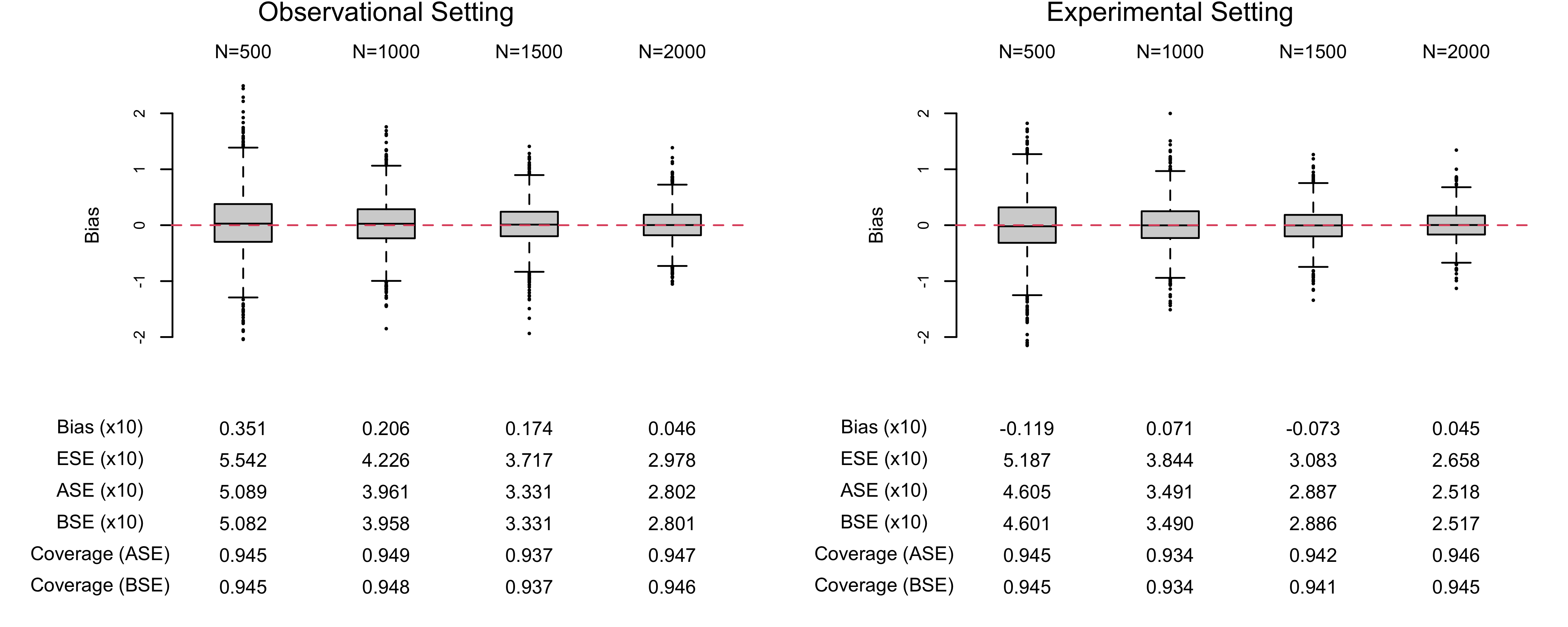
Figure 2: A Graphical Summary of the Simulation Results. The left and right panels show results for observational and experimental settings, respectively. In the top panel, each column gives boxplots of biases of the proposed estimator of ${\tau}_{\text{CSE}}^{*}(a_{D}=0)$ for $N\in\{500,1000,1500,2000\}$, respectively. The bottom panel provides numerical summaries informing the performance of the proposed estimator. Each row represents the empirical bias, empirical standard error (ESE), asymptotic standard error based on the proposed variance estimator (ASE), bootstrap standard error (BSE), empirical coverage rates of 95% confidence intervals based on the ASE and BSE. The bias and standard errors are scaled by factors of 10.

6 Application: The Southwest Oncology Group Trial

We reanalyzed data from the Southwest Oncology Group Trial (SWOG) (Petrylak et al., 2004). We used data from 487 male patients aged 47 to 88 years with refractory prostate cancer who were randomly assigned to one of two chemotherapies: Estramustine and Docetaxel (ED) or Prednisone and Mitoxantrone (PM), which are denoted by $A=1$ and $A=0$, respectively. Before being assigned to cancer chemotherapy, the following six variables were measured for each patient: type of progression, degree of bone pain, SWOG performance measure, race, age, and quality of life. At one-year follow-up, quality of life was measured again, but this follow-up was available only for patients who had survived up to the follow-up period.

The SWOG trial dataset has been used to study the effect of each chemotherapy on health-related quality of life, e.g., by Ding et al. (2011); Wang et al. (2017); Yang and Ding (2018); Stensrud et al. (2022a), who used the same outcome $Y$, defined as the change in quality of life between the baseline and follow-up periods. However, they focused on different causal effects. Specifically, the first three papers evaluated the causal effect of ED versus PM on the change in quality of life in the principal stratum of always survivors, i.e., the survivor average causal effect. In contrast, Stensrud et al. (2022a) focused on evaluating a CSE of ED versus PM on the change in quality of life, with specific details outlined below.

First, $A_{Y}=1$ and $A_{Y}=0$ indicate receiving only the Estramustine component of ED and the Prednisone component of PM, respectively. As primarily palliative and pain relief medications, there is no clear evidence that Estramustine and Prednisone offer any survival benefit. Therefore, it is reasonable to assume that ED and PM do not have a direct effect on mortality. Estramustine and Prednisone might also induce side effects like nausea, fatigue, and vomiting (Petrylak et al., 2004; Petrylak, 2005; Autio et al., 2012). The pain relief properties and the potential for side effects can ultimately influence an individual’s overall quality of life. We use this argument to justify Assumption (A4)-(ii), $A_{Y}$-partial isolation, which is not guaranteed by the experimental design.

Second, $A_{D}=1$ and $A_{D}=0$ indicate receiving only the Docetaxel component of ED and the Mitoxantrone component of PM, respectively. This choice was motivated by the fact that Docetaxel and Mitoxantrone are chemotherapeutic agents that can inhibit cancer cell proliferation and reduce the risk of death during the study period. However, it is plausible that these drugs affect quality of life through cancer progression. If this is the case, it implies the existence of a causal relationship between $A_{D}$ and the outcome variable $Y$, thus violating Assumption (A4)-(i), $A_{D}$-partial isolation. Under such circumstances, the CSE defined below can be viewed as a direct effect of $A_{D}$ on $Y$, but it may not capture all of the effects of $A_{D}$ on $Y$.

Assuming (A4)-(ii), $A_{Y}$-partial isolation, Stensrud et al. (2022a) focused on the following CSE:

$$\tau_{\text{CSE}}^{*}(a_{D}=\text{Docetaxel})$$

$$=\psi^{*}(a_{Y}=\text{Prednisone},\,a_{D}=\text{Docetaxel})-\psi^{*}(a_{Y}=\text{Estramustine},\,a_{D}=\text{Docetaxel})$$

$$=E\big{\{}Y^{(a_{Y}=\text{Prednisone},\,a_{D}=\text{Docetaxel})}-Y^{(a_{Y}=\text{Estramustine},\,a_{D}=\text{Docetaxel})}\,\big{|}\,D^{(a_{D}=\text{Docetaxel})}=0\big{\}}\ .$$

In words, $(a_{Y}=\text{Prednisone},\,a_{D}=\text{Docetaxel})$ (PD) is a combination of the component of ED that affects mortality (i.e., Docetaxel) and that of PM that may directly affect quality of life (i.e., Prednisone). Therefore, $\tau_{\text{CSE}}^{*}(\text{Docetaxel})$ quantifies the causal effect of receiving Prednisone over Estramustine among patients who would survive had they received Docetaxel as part of their treatment. For identification and estimation of $\tau_{\text{CSE}}^{*}(\text{Docetaxel})$, Stensrud et al. (2022a) relied on the assumption that there is no unmeasured confounding between death and the change in quality of life. However, it is important to acknowledge the potential presence of such unmeasured variables, including medical history, chronic diseases, lifestyle factors (e.g., smoking, drinking, physical activity), disease progression, and complications.

In order to address the potential for unmeasured confounding, we estimated $\tau_{\text{CSE}}^{*}(\text{Docetaxel})$ using the proposed approach. Specifically, as cancer chemotherapies were randomly assigned, we implemented the version of the proposed methods tailored for experimental settings, detailed in Section A.11 of the Supplementary Material. For the proxy variables $W$ and $Z$, we used quality of life and age, respectively, and the remaining four pre-treatment covariates as $X$. The choice of $Z$ was motivated by the hypothesis that age may affect mortality but may not directly affect the change in quality of life conditional on $X$ and potential unmeasured confounders $U$. Likewise, the choice of $W$ was based on the rationale that baseline quality of life could affect the change in quality of life but not directly affect mortality conditional on $X$ and $U$. Test statistics for pairwise partial correlations between $W$ and $Z$ given $X$ indicated that $U$ is likely present in the context; see Section A.13.1 of the Supplementary Material for details. As in the simulation study, we selected hyperparameters based on 5-fold cross-validation. To mitigate particular random split on these estimates, we adopted the median adjustment by repeating cross-fitting 200 times, see Section A.8 of the Supplementary Material for details. We imputed missing outcomes by Multivariate Imputation by Chained Equations (MICE) algorithm implemented in mice R-package (van Buuren and Groothuis-Oudshoorn, 2011). We note that MICE requires the missing at random assumption, and the results presented below remain consistent even when the analysis is restricted to patients with complete data; see Section A.13.3 of the Supplementary Material for details. Lastly, for comparison, we also estimated $\tau_{\text{CSE}}^{*}(\text{Docetaxel})$ assuming that there is no unmeasured common cause of death and the change in quality of life; see Section A.13.2 of the Supplementary Material for details.

Table 1 summarizes the result. First, the estimate of $\psi^{*}(\text{Prednisone,Docetaxel})$, the expected change in quality of life of receiving Prednision among patients who would survive had they received Docetaxel as part of their treatment, accounting for $U$ was -7.97, which is larger than the estimate obtained by assuming no $U$, -6.25. On the other hand, the estimate of ${\psi}^{*}(\text{Estramustine,Docetaxel})$, the expected change in quality of life of receiving Estramustine among patients who would survive had they received Docetaxel as part of their treatment, is equal to -4.71 in both approaches, because it can be simply estimated by the sample mean due to randomization; see Section A.11.3 of the Supplementary Material for details. Furthermore, the estimate of $\tau_{\text{CSE}}^{*}(\text{Decetaxel})$ under the proximal approach, -3.23, is larger than that assuming no $U$, -1.50. At the 5% level, both approaches conclude that ${\psi}^{*}(\text{Prednisone,Docetaxel})$ is significantly different from 0 whereas ${\psi}^{*}(\text{Estramustine,Docetaxel})$ and $\tau_{\text{CSE}}^{*}(\text{Decetaxel})$ are not significantly different from 0. Therefore, it appears that there is no significant difference between the effects of Prednisone and Estramustine on the change in quality of life in the subgroup of patients who would have survived with Docetaxel treatment, even after accounting for the potential for unmeasured common causes of death and quality of life. This conclusion agrees with the findings presented in Stensrud et al. (2022a).

Allow for $U$	Statistic	Estimand
		$\psi^{*}(\text{Prednisone},\text{Docetaxel})$	$\psi^{*}(\text{Estramustine},\text{Docetaxel})$	$\tau_{\text{CSE}}^{*}(\text{Docetaxel})$
Yes	Estimate	-7.97	-4.71	-3.23
	ASE	3.05	1.47	3.31
	95% CI	(-13.95, -1.98)	(-7.59, -1.84)	(-9.73, 3.26)
No	Estimate	-6.25	-4.71	-1.50
	ASE	2.36	1.47	2.63
	95% CI	(-10.88, -1.62)	(-7.59, -1.84)	(-6.65, 3.66)

Table 1: Summary Statistics of the Estimation of the CSE $\tau_{\text{CSE}}^{*}(\text{Decetaxel})$. Statistics in “Allow for $U$=Yes” and “Allow for $U$=No” rows are obtained from the proximal approach proposed in Section A.11 and from the approach proposed in Section A.13.2 developed under unconfoundedness (i.e., without $U$), respectively. ASE and 95% CI stand for the asymptotic standard error obtained from the proposed consistent variance estimator and the corresponding 95% confidence intervals, respectively.

7 Concluding Remarks

We have proposed a proximal causal inference framework for identifying and estimating the CSE in the presence of unmeasured confounding. This framework includes a locally semiparametric efficient influence function for the CSE under model $\mathcal{M}$ at submodel $\mathcal{M}_{\text{sub}}$. Using this efficient influence function, we constructed a semiparametric estimator of the CSE with all nuisance components estimated nonparametrically. We established that the estimator exhibits a mixed-bias structure in the sense that the estimator is consistent and asymptotically normal if some, but not necessarily all, nuisance components are estimated at sufficiently fast rates. We demonstrated the theoretical properties of the estimator in simulation studies, and then applied our method to a real-world randomized trial to evaluate the effect of cancer chemotherapies on the change in quality of life.

In many real-world applications, it is plausible that a rich collection of post-treatment time-varying covariates is available, with units experiencing missing data for reasons unrelated to the post-treatment event in view. While the proposed framework does not incorporate time-varying covariates beyond the post-treatment event, their inclusion is of substantial importance for researchers studying longitudinal data. We plan to accommodate time-varying covariates and missing data in future work, thereby expanding the applicability of our approach to general longitudinal settings.

The proposed approach hinges on the plausibility of separable treatments, which, e.g., could be decompositions of the original study treatment, that exert particular causal effects. In some studies, such as the SWOG trial, the treatment actually consists of two distinct components. Then the treatment decomposition seems to be concrete and plausible. However, in cases where the original treatment is not explicitly defined as a composite of two components, a justification for the decomposition is necessary. This justification should be guided by subject-matter expertise, as we generally want the estimand to correspond to practically relevant research questions. Furthermore, the exercise of articulating decompositions can itself be useful for sharpening research questions, enriching the understanding of the treatment mechanisms, and inspiring future treatment strategies (Robins and Richardson, 2011; Robins et al., 2022; Stensrud et al., 2021, 2022a, 2022b).

Supplementary Material

This document contains supplementary materials for “Proximal Causal Inference for Conditional Separable Effects.” Section A presents additional results related to the main paper. Section B presents proofs of the theorems in the main paper.

Appendix A Details of the Main Paper

A.1 Conditional Independencies of the Observed Variables

We will use the following conditional independencies of the observed variables in Section B, which are satisfied under Assumptions (A1) and (A6):

• $Y\rotatebox[origin={c}]{90.0}{$\models$}Z\,\big{|}\,A,D,X,U$

• $D\rotatebox[origin={c}]{90.0}{$\models$}Z\,\big{|}\,A,X,U$

• $W\rotatebox[origin={c}]{90.0}{$\models$}(A,Z)\,\big{|}\,D,X,U$

• $W\rotatebox[origin={c}]{90.0}{$\models$}(A,D,Z)\,\big{|}\,X,U$

• $W\rotatebox[origin={c}]{90.0}{$\models$}Z\,\big{|}\,A,D,X,U$

• $W\rotatebox[origin={c}]{90.0}{$\models$}Z\,\big{|}\,A,X,U$

To establish the result, we first introduce the graphoid axioms of conditional independence for random variables (Dawid, 1979).

• $S_{1}\rotatebox[origin={c}]{90.0}{$\models$}S_{2}\,\big{|}\,S_{3}$ $\Rightarrow$ $S_{2}\rotatebox[origin={c}]{90.0}{$\models$}S_{1}\,\big{|}\,S_{3}$

• $S_{1}\rotatebox[origin={c}]{90.0}{$\models$}(S_{2},S_{3})\,\big{|}\,S_{4}$ $\Rightarrow$ $S_{1}\rotatebox[origin={c}]{90.0}{$\models$}S_{2}\,\big{|}\,S_{4}$ and $S_{1}\rotatebox[origin={c}]{90.0}{$\models$}S_{3}\,\big{|}\,S_{4}$

• $S_{1}\rotatebox[origin={c}]{90.0}{$\models$}(S_{2},S_{3})\,\big{|}\,S_{4}$ $\Rightarrow$ $S_{1}\rotatebox[origin={c}]{90.0}{$\models$}S_{2}\,\big{|}\,(S_{3},S_{4})$

• $S_{1}\rotatebox[origin={c}]{90.0}{$\models$}S_{2}\,\big{|}\,S_{3}$ and $S_{1}\rotatebox[origin={c}]{90.0}{$\models$}S_{4}\,\big{|}\,(S_{2},S_{3})$ $\Rightarrow$ $S_{1}\rotatebox[origin={c}]{90.0}{$\models$}(S_{2},S_{4})\,\big{|}\,S_{3}$

We now establish conditions (CI1)-(CI6). First, (CI1) is established as follows:

(A6)-(i) + (A6)-(ii)

$$\Rightarrow\quad Z\rotatebox[origin={c}]{90.0}{$\models$}(Y^{(A)},D^{(A)})\,\big{|}\,(A,X,U) \Leftarrow\quad\text{\hyperlink{(G4)}{(G4)}}$$

$$\Rightarrow\quad Z\rotatebox[origin={c}]{90.0}{$\models$}(Y,D)\,\big{|}\,(A,X,U) \Leftarrow\quad\text{\hyperlink{(A1)}{(A1)}}$$

$$\Rightarrow\quad Z\rotatebox[origin={c}]{90.0}{$\models$}Y\,\big{|}\,(A,D,X,U) \Leftarrow\quad\text{\hyperlink{(G3)}{(G3)}}$$

Next, (CI2) is trivial from (A1) and (A6)-(ii). Lastly, (CI3), (CI4), (CI5), and (CI6) are established as follows:

(A6)-(iii) + (A6)-(iv)

$$\Rightarrow\quad W\rotatebox[origin={c}]{90.0}{$\models$}(A,D^{(A)},Z)\,\big{|}\,(X,U) \Leftarrow\quad\text{\hyperlink{(G4)}{(G4)}}$$

$$\Rightarrow\quad W\rotatebox[origin={c}]{90.0}{$\models$}(D^{(A)},Z)\,\big{|}\,(A,X,U) \Leftarrow\quad\text{\hyperlink{(A6)}{(A6)}-(iii)}$$

$$\Rightarrow\quad\text{\hyperlink{(CI6)}{(CI6)}: }W\rotatebox[origin={c}]{90.0}{$\models$}(D,Z)\,\big{|}\,(A,X,U) \Leftarrow\quad\text{\hyperlink{(A1)}{(A1)}}$$

$$\Rightarrow\quad\text{\hyperlink{(CI4)}{(CI4)}: }W\rotatebox[origin={c}]{90.0}{$\models$}(A,D,Z)\,\big{|}\,(X,U) \Leftarrow\quad\text{\hyperlink{(G4)}{(G4)} and $W\rotatebox[origin={c}]{90.0}{$\models$}A\,\big{|}\,(X,U)$ in the second line}$$

$$\Rightarrow\quad\text{\hyperlink{(CI3)}{(CI3)}: }W\rotatebox[origin={c}]{90.0}{$\models$}(A,Z)\,\big{|}\,(D,X,U) \Leftarrow\quad\text{\hyperlink{(G3)}{(G3)}}$$

$$\Rightarrow\quad\text{\hyperlink{(CI5)}{(CI5)}: }W\rotatebox[origin={c}]{90.0}{$\models$}Z\,\big{|}\,(A,D,X,U) \Leftarrow\quad\text{\hyperlink{(G3)}{(G3)}}$$

Next, we establish (CI1), (CI-3)-(CI-6) under Assumptions (A2’) (see Section A.11) and (A6)-(i), (iii), (iv). From, Assumption (A2’), we find the density of $Z\,\big{|}\,A,D^{(a)},X,U$ is

$$f^{*}(Z=z,Y^{(a)}=y\,\big{|}\,A,D^{(a)},X,U)$$

$$=\frac{f^{*}(Z=z,Y^{(a)}=y,A,D^{(a)},X,U)}{f^{*}(A,D^{(a)},X,U)}$$

$$=\frac{f^{*}(Z=z,Y^{(a)}=y,D^{(a)},X,U)f^{*}(A)}{f^{*}(D^{(a)},X,U)f^{*}(A)} \Leftarrow\quad\text{\hyperlink{(A2')}{(A2')}}$$

$$=\frac{f^{*}(Z=z,Y^{(a)}=y,D^{(a)},X,U)f^{*}(A=a)}{f^{*}(D^{(a)},X,U)f^{*}(A=a)}$$

$$=\frac{f^{*}(Z=z,Y^{(a)}=y,A=a,D^{(a)},X,U)}{f^{*}(A=a,D^{(a)},X,U)} \Leftarrow\quad\text{\hyperlink{(A2')}{(A2')}}$$

$$=\frac{f^{*}(Z=z,Y=y,A=a,D,X,U)}{f^{*}(A=a,D,X,U)} \Leftarrow\quad\text{\hyperlink{(A1)}{(A1)}}$$

$$=f^{*}(Z=z,Y=y\,\big{|}\,A=a,D,X,U)\ .$$ (17)

Similarly, we establish

$$f^{*}(Z=z\,\big{|}\,A,D^{(a)},X,U)=f^{*}(Z=z\,\big{|}\,A=a,D,X,U)$$ (18)

$$f^{*}(Y^{(a)}=y\,\big{|}\,A,D^{(a)},X,U)=f^{*}(Y=y\,\big{|}\,A=a,D,X,U)\ .$$ (19)

Therefore, we obtain the following result for all $a=0,1$:

$$f^{*}(Z=z,Y=y\,\big{|}\,A=a,D,X,U)$$

$$=f^{*}(Z=z,Y^{(a)}=y\,\big{|}\,A,D^{(a)},X,U) \Leftarrow\quad\eqref{eq-CI11}$$

$$=f^{*}(Z=z\,\big{|}\,A,D^{(a)},X,U)f^{*}(Y^{(a)}=y\,\big{|}\,A,D^{(a)},X,U) \Leftarrow\quad\text{\hyperlink{(A6)}{(A6)}-(i)}$$

$$=f^{*}(Z=z\,\big{|}\,A=a,D,X,U)f^{*}(Y=y\,\big{|}\,A=a,D,X,U) \Leftarrow\quad\eqref{eq-CI12},\eqref{eq-CI13}$$

which implies (CI1): $Y\rotatebox[origin={c}]{90.0}{$\models$}Z\,\big{|}\,A,D,X,U$. Conditions (CI3)-(CI6) can be established under Assumptions (A2’) and (A6)-(i), (iii), (iv) based on the same reasons.

A.2 Details of the Representation of $\psi^{*}(a_{Y},a_{D})$

We provide the details of (4). We find

$$E\big{\{}Y^{(a_{Y},a_{D}=1)}\,\big{|}\,D^{(a_{Y},a_{D}=1)}=0,X,U\big{\}}$$

$$=E\big{\{}Y^{(a_{Y},a_{D}=1)}\,\big{|}\,D^{(a_{Y},a_{D}=1)}=0,A_{Y}(G)=a_{Y},A_{D}(G)=1,X,U\big{\}}$$

$$=E\big{\{}Y(G)\,\big{|}\,D(G)=0,A_{Y}(G)=a_{Y},A_{D}(G)=1,X,U\big{\}}$$

$$=E\big{\{}Y(G)\,\big{|}\,D(G)=0,A_{Y}(G)=a_{Y},A_{D}(G)=0,X,U\big{\}}$$

$$=E\big{\{}Y^{(a_{Y},a_{D}=0)}\,\big{|}\,D^{(a_{Y},a_{D}=0)}=0,A_{Y}(G)=a_{Y},A_{D}(G)=0,X,U\big{\}}$$

$$=E\big{\{}Y^{(a_{Y},a_{D}=0)}\,\big{|}\,D^{(a_{Y},a_{D}=0)}=0,X,U\big{\}}\ .$$ (20)

The second line holds from the fact that $A_{Y}(G)$ and $A_{D}(G)$ are randomized. The third line holds from the consistency (A1). The fourth line holds from (A5)-(i). The last two lines can be easily deduced by the same reasons. Therefore,

$$E\big{\{}Y^{(a_{Y},a_{D})}\,\big{|}\,D^{(a_{Y},a_{D})}=0,X,U\big{\}}$$

$$=E\big{\{}Y^{(a_{Y},a_{D}=a_{Y})}\,\big{|}\,D^{(a_{Y},a_{D}=a_{Y})}=0,X,U\big{\}}$$

$$=E\big{\{}Y^{(a_{Y})}\,\big{|}\,D^{(a_{Y})}=0,X,U\big{\}}$$

$$=\int y\frac{f^{*}(Y^{(a_{Y})}=y,D^{(a_{Y})}=0\,\big{|}\,X=x,U=u)}{\Pr\{D^{(a_{Y})}=0\,\big{|}\,X=x,U=u\}}\,f^{*}(X=x,U=u)\,d(x,u)$$

$$=\int y\frac{f^{*}(Y^{(a_{Y})}=y,D^{(a_{Y})}=0\,\big{|}\,A=a_{Y},X=x,U=u)}{\Pr\{D^{(a_{Y})}=0\,\big{|}\,A=a_{Y},X=x,U=u\}}\,f^{*}(X=x,U=u)\,d(x,u)$$

$$=\int y\frac{f^{*}(Y=y,D=0\,\big{|}\,A=a_{Y},X=x,U=u)}{\Pr(D=0\,\big{|}\,A=a_{Y},X=x,U=u)}\,f^{*}(X=x,U=u)\,d(x,u)$$

$$=E\big{(}Y\,\big{|}\,A=a_{Y},D=0,X,U\big{)}\ .$$ (21)

The second line is from (20). The third line is from the relationship between the two-arm study and the four-arm trial. The fourth line is from the definition of the conditional expectation. The fifth line is from Assumption (A2). The sixth line is from Assumption (A1). The last line is from the definition of the conditional expectation.

Similarly, we have

$$\Pr\big{\{}D^{(a_{Y}=1,a_{D})}=0\,\big{|}\,X,U\big{\}}$$

$$=\Pr\big{\{}D^{(a_{Y}=1,a_{D})}=0\,\big{|}\,A_{Y}=1,A_{D}=a_{D},X,U\big{\}}$$

$$=\Pr\big{\{}D(G)=0\,\big{|}\,A_{Y}=1,A_{D}=a_{D},X,U\big{\}}$$

$$=\Pr\big{\{}D(G)=0\,\big{|}\,A_{Y}=0,A_{D}=a_{D},X,U\big{\}}$$

$$=\Pr\big{\{}D^{(a_{Y}=0,a_{D})}=0\,\big{|}\,X,U\big{\}}\ .$$ (22)

The two line holds from the fact that $A_{Y}(G)$ and $A_{D}(G)$ are randomized. The third line holds from the consistency (A1). The fourth line holds from (A5)-(ii). The last line can be easily deduced by reversing the order of the first four lines. Therefore,

$$\Pr\big{\{}D^{(a_{Y},a_{D})}=0\,\big{|}\,X,U\big{\}}$$

$$=\Pr\big{\{}D^{(a_{Y}=a_{D},a_{D})}=0\,\big{|}\,X,U\big{\}}$$

$$=\Pr\big{\{}D^{(a_{D})}=0\,\big{|}\,X,U\big{\}}$$

$$=\Pr\big{\{}D^{(a_{D})}=0\,\big{|}\,A=a_{D},X,U\big{\}}$$

$$=\Pr\big{(}D=0\,\big{|}\,A=a_{D},X,U\big{)}\ .$$ (23)

The second line is from (A.2). The third line is from the relationship between the two-arm study and the four-arm trial. The fourth line is from Assumption (A2). The last line is from Assumption (A1).

Therefore, $\psi^{*}(a_{Y},a_{D})$ is represented as

$$\psi^{*}(a_{Y},a_{D})$$

$$=E\big{[}E\big{\{}Y^{(a_{Y},a_{D})}\,\big{|}\,D^{(a_{Y},a_{D})}=0,X,U\big{\}}\,\big{|}\,D^{(a_{Y},a_{D})}=0\big{]}$$

$$=E\big{\{}E\big{(}Y\,\big{|}\,A=a_{Y},D=0,X,U\big{)}\,\big{|}\,D^{(a_{Y},a_{D})}=0\big{\}}$$

$$=\frac{E\big{[}E\big{(}Y\,\big{|}\,A=a_{Y},D=0,X,U\big{)}\mathbbm{1}\big{\{}D^{(a_{Y},a_{D})}=0\big{\}}\big{]}}{E\big{[}\mathbbm{1}\big{\{}D^{(a_{Y},a_{D})}=0\big{\}}\big{]}}$$

$$=\frac{E\big{[}E\big{(}Y\,\big{|}\,A=a_{Y},D=0,X,U\big{)}\Pr\big{\{}D^{(a_{Y},a_{D})}=0\,\big{|}\,X,U\big{\}}\big{]}}{E\big{[}\Pr\big{\{}D^{(a_{Y},a_{D})}=0\,\big{|}\,X,U\big{\}}\big{]}}$$

$$=\frac{E\big{\{}E\big{(}Y\,\big{|}\,A=a_{Y},D=0,X,U\big{)}\Pr\big{(}D=0\,\big{|}\,A=a_{D},X,U\big{)}\big{\}}}{E\big{\{}\Pr\big{(}D=0\,\big{|}\,A=a_{D},X,U\big{)}\big{\}}}$$

The second line is from the law of iterated expectation. The third line is from (21). The fourth and fifth lines are trivial from the definition of the conditional expectation and the law of iterated expectation. The last line is from (23).

A.3 Sufficient Conditions for the Existence of the Bridge Function

In this subsection, we provide sufficient conditions for the existence of the synthetic control bridge function $h^{*}$. In brief, we follow the approach in Miao et al. (2018). The proof relies on Theorem 15.18 of Kress (2014), which is stated below for completeness.
Theorem 15.18. (Kress, 2014) Let $A:X\rightarrow Y$ be a compact operator with singular system $\big{\{}\mu_{n},\phi_{n},g_{n}\big{\}}_{n=1,2,\ldots}$. The integral equation of the first kind $A\phi=f$ is solvable if and only if

• $f\in\mathcal{N}(A^{\text{adjoint}})^{\perp}=\big{\{}f\,\big{|}\,A^{\text{adjoint}}(f)=0\big{\}}^{\perp}$;

• $\sum_{n=1}^{\infty}\mu_{n}^{-2}\big{|}\langle f,g_{n}\rangle|^{2}<\infty$

We only discuss the existence of the solution to integral equation (5), but the existence of the solution to the other integral equations can be established in a similar fashion. For notational brevity, we denote $g_{x}^{*}(z):=E\big{(}Y\,\big{|}\,Z=z,A=a_{Y},D=0,X=x)$.

To apply the Theorem, we introduce some additional notations. For a fixed $X=x$, let $\mathcal{L}_{W}=\mathcal{L}_{2}(W,A=a_{Y},D=0,X=x)$ and $\mathcal{L}_{Z}=\mathcal{L}_{2}(Z,A=a_{Y},D=0,X=x)$ be the spaces of square-integrable functions of $W$ and $Z$ given $(A=a_{Y},D=0,X=x)$ and $(A=a_{Y},D=0,X=x)$, respectively, which are equipped with the inner products

$$\langle h,h^{\prime}\rangle_{W}=\int h(w)h^{\prime}(w)\,f_{W|ADX}(w\,\big{|}\,a_{Y},0,x)\,dw=E\big{\{}h(W)h^{\prime}(W)\,\big{|}\,A_{Y}=a_{Y},D=0,X=x\big{\}}$$

$$\langle g,g^{\prime}\rangle_{Z}=\int g(z)g^{\prime}(z)\,f_{Z|ADX}(z\,\big{|}\,a_{Y},0,x)\,dz=E\big{\{}g(Z)g^{\prime}(Z)\,\big{|}\,A_{Y}=a_{Y},D=0,X=x\big{\}}$$

Let $\mathcal{K}_{x}:\mathcal{L}_{W}\rightarrow\mathcal{L}_{Z}$ be the conditional expectation of $h(W)\in\mathcal{L}_{W}$ given $(Z,A=a_{Y},D=0,X=x)$, i.e.,

$$\mathcal{K}_{x}(h)\in\mathcal{L}_{W}\text{ satisfying }\big{(}\mathcal{K}_{x}(h)\big{)}(Z)=E\big{\{}h(W)\,\big{|}\,Z,A=a_{Y},D=0,X=x\big{\}}\text{ for }h\in\mathcal{L}_{W}$$

Then, the bridge function $h_{1,x}^{*}\in\mathcal{L}_{W}$ solves $\mathcal{K}_{x}(h_{1,x}^{*})$, i.e.,

$$\int h_{1,x}^{*}(w)f_{W|ZADX}(w\,\big{|}\,z,a_{Y},0,x)\,dw=g_{x}^{*}(z),\ \forall z\ .$$

Now, we assume the following conditions for all $x$:

• (Bridge1) $\iint f_{W|ZADX}(w\,\big{|}\,z,a_{Y},0,x)f_{Z|WADX}(z\,\big{|}\,w,a_{Y},0,x)\,dw\,dz<\infty$;

• (Bridge2) For $g\in\mathcal{L}_{Z}$, $E\big{\{}g(Z)\,\big{|}\,W,A=a_{Y},D=0,X=x\big{\}}=0$ implies $g(Z)=0$ almost surely;

• (Bridge3) $E\big{[}\{g_{x}^{*}(Z)\}^{2}\,\big{|}\,A=a_{Y},D=0,X=x\big{]}<\infty$ almost surely;

• (Bridge4) Let the singular system of $\mathcal{K}_{x}$ be $\big{\{}\mu_{n,x},\phi_{n,x},g_{n,x}\big{\}}_{n=1,2,\ldots}$. Then, we have $\sum_{n=1}^{\infty}\mu_{n,x}^{-2}\big{|}\langle g_{x}^{*}(Z),g_{n,x}\rangle_{Z}|^{2}<\infty$.

First, we show that $\mathcal{K}$ is a compact operator under Condition (Bridge1). Let $\mathcal{K}^{\text{adjoint}}:\mathcal{L}_{Z}\rightarrow\mathcal{L}_{W}$ be the conditional expectation of $g(Z)\in\mathcal{L}_{Z}$ given $(W,A=a_{Y},D=0,X=x)$, i.e.,

$$\mathcal{K}_{x}^{\text{adjoint}}(g)\in\mathcal{L}_{W}\text{ satisfying }\big{(}\mathcal{K}_{x}(g)\big{)}(W)=E\big{\{}g(Z)\,\big{|}\,W,A=a_{Y},D=0,X=x\big{\}}\text{ for }g\in\mathcal{L}_{Z}$$

Then, $\mathcal{K}_{x}$ and $\mathcal{K}_{x}^{\text{adjoint}}$ are the adjoint operator of each other as follows:

$$\langle\mathcal{K}_{x}(h),g\rangle_{Z}$$

$$=E\Big{[}E\big{\{}h(W)\,\big{|}\,Z,A=a_{Y},D=0,X=x\big{\}}g(Z)\,\Big{|}\,A=a_{Y},D=0,X=x\Big{]}$$

$$=E\Big{[}h(W)g(Z)\,\Big{|}\,A=a_{Y},D=0,X=x\Big{]}$$

$$=E\Big{[}h(W)E\big{\{}g(Z)\,\big{|}\,W,A=a_{Y},D=0,X=x\big{\}}\Big{]}$$

$$=\langle h,\mathcal{K}_{x}^{\text{adjoint}}(g)\rangle_{W}$$

Additionally, as shown in page 5659 of Carrasco et al. (2007), $\mathcal{K}_{x}$ and $\mathcal{K}_{x}^{\text{adjoint}}$ are compact operators under Condition (Bridge1). Moreover, by Theorem 15.16 of Kress (2014), there exists a singular value decomposition of $\mathcal{K}_{x}$ as $\big{\{}\mu_{n,x},\phi_{n,x},g_{n,x}\big{\}}_{n=1,2,\ldots}$.

Second, we show that $\mathcal{N}(\mathcal{K}_{x}^{\text{adjoint}})^{\perp}=\mathcal{L}_{Z}$, which suffices to show $\mathcal{N}(\mathcal{K}_{x}^{\text{adjoint}})=\big{\{}0\big{\}}\subseteq\mathcal{L}_{Z}$. Under Condition (Bridge2), we have

$$g\in\mathcal{N}(\mathcal{K}_{x}^{\text{adjoint}})\quad\Rightarrow\quad E\big{\{}g(Z)\,\big{|}\,W=w,A=a_{Y},D=0,X=x\big{\}}=0,\ \forall w\quad\Rightarrow\quad g(Z)=0$$

where the first arrow is from the definition of the null space $\mathcal{N}$, and the second arrow is from Condition (Bridge2). Therefore, any $g\in\mathcal{N}(\mathcal{K}_{x}^{\text{adjoint}})$ must satisfy $g(Z)=0$ almost surely, i.e., $\mathcal{N}(\mathcal{K}_{x}^{\text{adjoint}})=\big{\{}0\big{\}}\subseteq\mathcal{L}_{Z}$ almost surely.

Third, it is trivial that $g_{x}^{*}(Z)\in\mathcal{L}_{Z}=\mathcal{N}(\mathcal{K}_{x}^{\text{adjoint}})^{\perp}$ under Condition (Bridge3).

Combining the three results, we establish that $g_{x}^{*}(Z)$ satisfies the first condition of Theorem 15.18 of Kress (2014). The second condition of the Theorem is exactly the same as Condition (Bridge4). Therefore, we establish that the Fredholm integral equation of the first kind $\mathcal{K}_{x}(h)=g_{x}^{*}(Z)$ is solvable under Conditions (Bridge1)-(Bridge4), i.e., for each $x$, there exists a function $h_{1,x}^{*}(w)$ satisfying

$$\int h_{1,x}^{*}(w)f_{W|ZADX}(w\,\big{|}\,z,a_{Y},0,x)\,dw=g_{x}^{*}(z),\ \forall z\ .$$

Therefore, $h_{1}^{*}(x,w):=h_{1,x}^{*}(w)$ satisfies

$$\int h_{1}^{*}(x,w)f_{W|ZADX}(w\,\big{|}\,z,a_{Y},0,x)\,dw=g^{*}(z,x),\ \forall(z,x)\ ,$$

implying that the bridge function exists.

A.4 Details of the Empirical Risk Minimization

We provide details on the construction of the empirical risk functions $\widehat{R}_{h1}$, $\widehat{R}_{h0}$, $\widehat{R}_{h2}$, $\widehat{R}_{q0}$, $\widehat{R}_{q0}$. First, we introduce Lemma 2 of Mastouri et al. (2021):
Lemma 2 (Mastouri et al., 2021): Let $\mathcal{K}(\cdot,\cdot)$ be the kernel of the RKHS of $q$. Suppose that

$$E\big{[}\mathbbm{1}(A=a_{Y},D=0)\big{\{}Y-h(W,X)\big{\}}^{2}\mathcal{K}((Z,X),(Z,X))\big{]}<\infty\ .$$ (24)

Then, we have

$$R_{h1}(h) =\max_{\begin{subarray}{c}q\in\mathcal{H}(Z,X)\\ q:\|q\|\leq 1\end{subarray}}\Big{[}E\big{[}q(Z,X)\mathbbm{1}(A=a_{Y},D=0)\big{\{}Y-h(W,X)\big{\}}\big{]}\Big{]}^{2}$$

$$=E\left[\begin{array}[]{l}\mathbbm{1}(A=a_{Y},D=0)\mathbbm{1}(A^{\prime}=a_{Y},D^{\prime}=0)\big{\{}Y-h(W,X)\big{\}}\big{\{}Y^{\prime}-h(W^{\prime},X^{\prime})\big{\}}\\ \times\mathcal{K}((Z,X),(Z^{\prime},X^{\prime}))\end{array}\right]\ .$$

The result is also reported in other works, e.g., Theorem 3.3 of Muandet et al. (2020) and Lemma 1 of Zhang et al. (2023). The condition (24) implies that $E\big{[}\mathbbm{1}(A=a_{Y},D=0)\big{\{}Y-h(W,X)\big{\}}\mathcal{K}((Z,X),\cdot)\big{]}$ is Bochner integrable (Steinwart and Christmann, 2008, Definition A.5.20). One important property of the Bochner integrability is that an integration and a linear operator can be interchanged. Therefore, we find

$$\max_{\begin{subarray}{c}q\in\mathcal{H}(Z,X)\\ q:\|q\|\leq 1\end{subarray}}\Big{[}{E}\big{[}q(Z,X)\mathbbm{1}(A=a_{Y},D=0)\big{\{}Y-h(W,X)\big{\}}\big{]}\Big{]}^{2}$$

$$=\max_{\begin{subarray}{c}q\in\mathcal{H}(Z,X)\\ q:\|q\|\leq 1\end{subarray}}\Big{[}{E}\big{[}\mathbbm{1}(A=a_{Y},D=0)\big{\{}Y-h(W,X)\big{\}}\langle q,\mathcal{K}((Z,X),\cdot)\rangle\big{]}\Big{]}^{2}$$

$$=\max_{\begin{subarray}{c}q\in\mathcal{H}(Z,X)\\ q:\|q\|\leq 1\end{subarray}}\Big{[}\Big{\langle}q,{E}\big{[}\mathbbm{1}(A=a_{Y},D=0)\big{\{}Y-h(W,X)\big{\}}\mathcal{K}((Z,X),\cdot)\big{]}\Big{\rangle}\Big{]}^{2}$$

$$=\Big{\|}{E}\big{[}\mathbbm{1}(A=a_{Y},D=0)\big{\{}Y-h(W,X)\big{\}}\mathcal{K}((Z,X),\cdot)\big{]}\Big{\|}_{\mathcal{H}(Z,X)}^{2}$$

$$=\Big{\langle}{E}\big{[}\mathbbm{1}(A=a_{Y},D=0)\big{\{}Y-h(W,X)\big{\}}\mathcal{K}((Z,X),\cdot)\big{]},$$

$$\hskip 28.45274pt{E}\big{[}\mathbbm{1}(A=a_{Y},D=0)\big{\{}Y-h(W,X)\big{\}}\mathcal{K}((Z,X),\cdot)\big{]}\Big{\rangle}$$

$$={E}\left[\begin{array}[]{l}\Big{\langle}\mathbbm{1}(A=a_{Y},D=0)\big{\{}Y-h(W,X)\big{\}}\mathcal{K}((Z,X),\cdot),\\ \hskip 28.45274pt{E}\big{[}\mathbbm{1}(A^{\prime}=a_{Y},D^{\prime}=0)\big{\{}Y^{\prime}-h(W^{\prime},X^{\prime})\big{\}}\mathcal{K}((Z^{\prime},X^{\prime}),\cdot)\big{]}\Big{\rangle}\end{array}\right]$$

$$={E}\left[\begin{array}[]{l}\Big{\langle}\mathbbm{1}(A=a_{Y},D=0)\big{\{}Y-h(W,X)\big{\}}\mathcal{K}((Z,X),\cdot),\\ \hskip 28.45274pt\mathbbm{1}(A^{\prime}=a_{Y},D^{\prime}=0)\big{\{}Y^{\prime}-h(W^{\prime},X^{\prime})\big{\}}\mathcal{K}((Z^{\prime},X^{\prime}),\cdot)\Big{\rangle}\end{array}\right]$$

$$=E\left[\begin{array}[]{l}\mathbbm{1}(A=a_{Y},D=0)\mathbbm{1}(A^{\prime}=a_{Y},D^{\prime}=0)\big{\{}Y-h(W,X)\big{\}}\big{\{}Y^{\prime}-h(W^{\prime},X^{\prime})\big{\}}\\ \quad\times\mathcal{K}((Z,X),(Z^{\prime},X^{\prime}))\end{array}\right]\ .$$

The second line holds from $q\in\mathcal{H}(Z,X)$, implying that $q(Z,X)=\langle q,\mathcal{K}((Z,X),\cdot)\rangle$. The third line holds from the Bochner integrability. The fourth line holds from the fact that $\mathcal{H}(Z,X)$ is a vector space, and ${E}\big{[}\big{\{}Y-h(W,X)\big{\}}\mathcal{K}((Z,X),\cdot)\big{]}\in\mathcal{H}(Z,X)$ from the Bochner integrability. Therefore, by choosing $q\propto{E}\big{[}\big{\{}Y-h(W,X)\big{\}}\mathcal{K}((Z,X),\cdot)\big{]}$, we obtain the result. The fifth line is trivial from the definition of the norm $\|\cdot\|_{\mathcal{H}(Z,X)}$. The sixth and seventh lines are from the Bochner integrability. The last line is trivial. Therefore, $\widehat{R}_{h1}^{(-k)}(h;a_{Y})$ in (12) is an empirical analogue of $R_{h1}(h;a_{Y})$.

The other empirical risk functions can be similarly constructed. Specifically, the population-level risk functions for $h_{0}^{*}$, $h_{2}^{*}$, $q_{0}^{*}$, and $q_{1}^{*}$ are

$$R_{h0}(h;a_{Y},a_{D})=E\left[\begin{array}[]{l}\mathbbm{1}(A=a_{D})\mathbbm{1}(A^{\prime}=a_{D})\big{\{}(1-D)h_{1}^{*}(W,X;a_{Y})-h(W,X)\big{\}}\\ \quad\times\big{\{}(1-D^{\prime})h_{1}^{*}(W^{\prime},X^{\prime};a_{Y})-h(W^{\prime},X^{\prime})\big{\}}\mathcal{K}\big{(}(Z,X),(Z^{\prime},X^{\prime})\big{)}\end{array}\right]\text{ if $a_{Y}\neq a_{D}$}$$

$$R_{h0}(h;a_{D},a_{D})=E\left[\begin{array}[]{l}\mathbbm{1}(A=a_{D})\mathbbm{1}(A^{\prime}=a_{D})\big{\{}Y(1-D)-h(W,X)\big{\}}\\ \quad\times\big{\{}Y^{\prime}(1-D^{\prime})-h(W^{\prime},X^{\prime})\big{\}}\mathcal{K}\big{(}(Z,X),(Z^{\prime},X^{\prime})\big{)}\end{array}\right]$$

$$R_{h2}(h;a_{D})=E\left[\begin{array}[]{l}\mathbbm{1}(A=a_{D})\mathbbm{1}(A^{\prime}=a_{D})\big{\{}(1-D)-h(W,X)\big{\}}\\ \quad\times\big{\{}(1-D^{\prime})-h(W^{\prime},X^{\prime})\big{\}}\mathcal{K}\big{(}(Z,X),(Z^{\prime},X^{\prime})\big{)}\end{array}\right]$$

$$R_{q0}(q;a_{D})=E\Big{[}\big{\{}1-\mathbbm{1}(A=a_{D})q(Z,W)\big{\}}\big{\{}1-\mathbbm{1}(A^{\prime}=a_{D})q(Z^{\prime},W^{\prime})\big{\}}\mathcal{K}\big{(}(W,X),(W^{\prime},X^{\prime})\big{)}\Big{]}$$

$$R_{q1}(q;a_{Y},a_{D})=E\left[\begin{array}[]{l}\mathbbm{1}(D=0)\mathbbm{1}(D^{\prime}=0)\\ \quad\times\big{\{}\mathbbm{1}(A=a_{D})q_{0}^{*}(Z,W)-\mathbbm{1}(A=a_{Y})q(Z,W)\big{\}}\\ \quad\times\big{\{}\mathbbm{1}(A^{\prime}=a_{D})q_{0}^{*}(Z^{\prime},W^{\prime})-\mathbbm{1}(A^{\prime}=a_{Y})q(Z^{\prime},W^{\prime})\big{\}}\\ \quad\times\mathcal{K}\big{(}(W,X),(W^{\prime},X^{\prime})\big{)}\end{array}\right]\ .$$

Therefore, the following empirical risk functions $\widehat{R}_{h0}^{(-k)}$, $\widehat{R}_{h2}^{(-k)}$, $\widehat{R}_{q0}^{(-k)}$, and $\widehat{R}_{q1}^{(-k)}$ are empirical analogues of the population-level risk functions:

$$\widehat{R}_{h0}^{(-k)}(h;a_{Y},a_{D})=\frac{1}{M_{k}^{2}}\sum_{i,j\in\mathcal{I}_{k}^{c}}\left[\begin{array}[]{l}\mathbbm{1}(A_{i}=a_{D},A_{j}=a_{D})\big{\{}(1-D_{i})\widehat{h}_{1}^{(-k)}(W_{i},X_{i};a_{Y})-h(W_{i},X_{i})\big{\}}\\ \quad\times\big{\{}(1-D_{j})\widehat{h}_{1}^{(-k)}(W_{j},X_{j};a_{Y})-h(W_{j},X_{j})\big{\}}\mathcal{K}\big{(}(Z_{i},X_{i}),(Z_{j},X_{j})\big{)}\end{array}\right]\text{ if $a_{Y}\neq a_{D}$}$$

$$\widehat{R}_{h0}^{(-k)}(h;a_{D},a_{D})=\frac{1}{M_{k}^{2}}\sum_{i,j\in\mathcal{I}_{k}^{c}}\left[\begin{array}[]{l}\mathbbm{1}(A_{i}=a_{D},A_{j}=a_{D})\big{\{}Y_{i}(1-D_{i})-h(W_{i},X_{i})\big{\}}\\ \quad\times\big{\{}Y_{j}(1-D_{j})-h(W_{j},X_{j})\big{\}}\mathcal{K}\big{(}(Z_{i},X_{i}),(Z_{j},X_{j})\big{)}\end{array}\right]$$

$$\widehat{R}_{h2}^{(-k)}(h;a_{D})=\frac{1}{M_{k}^{2}}\sum_{i,j\in\mathcal{I}_{k}^{c}}\left[\begin{array}[]{l}\mathbbm{1}(A_{i}=a_{D},A_{j}=a_{D})\big{\{}(1-D_{i})-h(W_{i},X_{i})\big{\}}\\ \quad\times\big{\{}(1-D_{j})-h(W_{j},X_{j})\big{\}}\mathcal{K}\big{(}(Z_{i},X_{i}),(Z_{j},X_{j})\big{)}\end{array}\right]$$

$$\widehat{R}_{q0}^{(-k)}(q;a_{D})=\frac{1}{M_{k}^{2}}\sum_{i,j\in\mathcal{I}_{k}^{c}}\left[\begin{array}[]{l}\big{\{}1-\mathbbm{1}(A_{i}=a_{D})q(Z_{i},X_{i})\big{\}}\\ \quad\times\big{\{}1-\mathbbm{1}(A_{j}=a_{D})q(Z_{j},X_{j})\big{\}}\mathcal{K}\big{(}(W_{i},X_{i}),(W_{j},X_{j})\big{)}\end{array}\right]$$

$$\widehat{R}_{q1}^{(-k)}(q;a_{Y},a_{D})=\frac{1}{M_{k}^{2}}\sum_{i,j\in\mathcal{I}_{k}^{c}}\left[\begin{array}[]{l}\mathbbm{1}(D_{i}=0,D_{j}=0)\\ \quad\times\big{\{}\mathbbm{1}(A_{i}=a_{D})\widehat{q}_{0}^{(-k)}(W_{i},Z_{i};a_{D})-\mathbbm{1}(A_{i}=a_{Y})q(Z_{i},W_{i})\big{\}}\\ \quad\times\big{\{}\mathbbm{1}(A_{j}=a_{D})\widehat{q}_{0}^{(-k)}(W_{j},Z_{j};a_{D})-\mathbbm{1}(A_{j}=a_{Y})q(Z_{j},W_{j})\big{\}}\\ \quad\times\mathcal{K}\big{(}(W_{i},X_{i}),(W_{j},X_{j})\big{)}\end{array}\right]\ .$$

We again note that, as best illustrated here, these empirical risk functions are motivated from the relationships (6)-(10). Due to the nested relationships, the empirical risk functions for $h_{0}^{*}$ and $q_{1}^{*}$ rely on the estimated bridge functions $\widehat{h}_{1}^{(-k)}$ and $\widehat{q}_{0}^{(-k)}$, respectively; we remark that a similar nonparametric approach for estimating nested functionals was considered in Singh (2022). The estimated bridge functions can be expressed in closed forms based on the representer theorem. Specifically, the empirical risk minimizers $\widehat{h}_{1}^{(-k)}$, $\widehat{h}_{0}^{(-k)}$, $\widehat{h}_{0}^{(-k)}$, $\widehat{q}_{0}^{(-k)}$, $\widehat{q}_{1}^{(-k)}$ are given as

$$\widehat{h}_{1}^{(-k)}(w,x;a_{Y})=\sum_{i\in\mathcal{I}_{k}^{c}}\widehat{\alpha}_{h1,i}(a_{Y})\mathcal{K}\big{(}(W_{i},X_{i}),(w,x)\big{)}\ ,$$

$$\widehat{h}_{0}^{(-k)}(w,x;a_{Y},a_{D})=\sum_{i\in\mathcal{I}_{k}^{c}}\widehat{\alpha}_{h0,i}(a_{Y},a_{D})\mathcal{K}\big{(}(W_{i},X_{i}),(w,x)\big{)}\text{ if $a_{Y}\neq a_{D}$}\ ,$$

$$\widehat{h}_{0}^{(-k)}(w,x;a_{D},a_{D})=\sum_{i\in\mathcal{I}_{k}^{c}}\widehat{\alpha}_{h0,i}(a_{D},a_{D})\mathcal{K}\big{(}(W_{i},X_{i}),(w,x)\big{)}\ ,$$

$$\widehat{h}_{2}^{(-k)}(w,x;a_{Y},a_{D})=\sum_{i\in\mathcal{I}_{k}^{c}}\widehat{\alpha}_{h2,i}(a_{D})\mathcal{K}\big{(}(W_{i},X_{i}),(w,x)\big{)}\ ,$$

$$\widehat{q}_{0}^{(-k)}(z,x;a_{D})=\sum_{i\in\mathcal{I}_{k}^{c}}\widehat{\alpha}_{q0,i}(a_{D})\mathcal{K}\big{(}(Z_{i},X_{i}),(z,x)\big{)}\ ,$$

$$\widehat{q}_{1}^{(-k)}(z,x;a_{Y},a_{D})=\sum_{i\in\mathcal{I}_{k}^{c}}\widehat{\alpha}_{q1,i}(a_{Y},a_{D})\mathcal{K}\big{(}(Z_{i},X_{i}),(z,x)\big{)}$$

where

$$\widehat{\alpha}_{h1}(a_{Y})=\big{\{}\mathcal{W}\mathcal{D}_{h1}(a_{Y})\mathcal{Z}\mathcal{D}_{h1}(a_{Y})\mathcal{W}+\lambda_{h1}\mathcal{W}\big{\}}^{-1}\big{\{}\mathcal{W}\mathcal{D}_{h1}(a_{Y})\mathcal{Z}\mathcal{Y}_{h1}\big{\}}$$

$$\widehat{\alpha}_{h0}(a_{Y},a_{D})=\big{\{}\mathcal{W}\mathcal{D}_{h0}(a_{D})\mathcal{Z}\mathcal{W}+\lambda_{h0}\mathcal{W}\big{\}}^{-1}\big{\{}\mathcal{W}\mathcal{D}_{h0}(a_{D})\mathcal{Z}\mathcal{Y}_{h0}(a_{Y},a_{D})\big{\}}$$

$$\widehat{\alpha}_{h0}(a_{D},a_{D})=\big{\{}\mathcal{W}\mathcal{D}_{h0}(a_{D})\mathcal{Z}\mathcal{D}_{h0}(a_{D})\mathcal{W}+\lambda_{h0}\mathcal{W}\big{\}}^{-1}\big{\{}\mathcal{W}\mathcal{D}_{h0}(a_{D})\mathcal{Z}\mathcal{Y}_{h0}(a_{D},a_{D})\big{\}}$$

$$\widehat{\alpha}_{h2}(a_{D})=\big{\{}\mathcal{W}\mathcal{D}_{h2}(a_{D})\mathcal{Z}\mathcal{D}_{h2}(a_{D})\mathcal{W}+\lambda_{h2}\mathcal{W}\big{\}}^{-1}\big{\{}\mathcal{W}\mathcal{D}_{h2}(a_{D})\mathcal{Z}\mathcal{Y}_{h2}\big{\}}$$

$$\widehat{\alpha}_{q0}(a_{D})=\big{\{}\mathcal{Z}\mathcal{D}_{q0}(a_{D})\mathcal{W}\mathcal{D}_{q0}(a_{D})\mathcal{Z}+\lambda_{q0}\mathcal{Z}\big{\}}^{-1}\big{\{}\mathcal{Z}\mathcal{D}_{q0}(a_{D})\mathcal{W}\mathcal{Y}_{q0}\big{\}}$$

$$\widehat{\alpha}_{q1}(a_{Y},a_{D})=\big{\{}\mathcal{Z}\mathcal{D}_{q1}(a_{Y})\mathcal{W}\mathcal{D}_{q1}(a_{Y})\mathcal{Z}+\lambda_{q1}\mathcal{Z}\big{\}}^{-1}\big{\{}\mathcal{Z}\mathcal{D}_{q1}(a_{Y})\mathcal{W}\mathcal{Y}_{q1}(a_{D})\big{\}}\ .$$

Here, $\mathcal{W}\in\mathbbm{R}^{M_{k}\times M_{k}}$ and $\mathcal{Z}\in\mathbbm{R}^{M_{k}\times M_{k}}$ are the gram matrices of which $(i,j)$th entries are $\mathcal{W}_{ij}=\mathcal{K}\big{(}(W_{i},X_{i}),(W_{j},X_{j})\big{)}$ and $\mathcal{Z}_{ij}=\mathcal{K}\big{(}(Z_{i},X_{i}),(Z_{j},X_{j})\big{)}$, respectively, and $\mathcal{D}\in\mathbbm{R}^{M_{k}\times M_{k}}$ are diagonal matrices with entries

$$\mathcal{D}_{h1}(a_{Y})=\text{diag}\Big{[}\mathbbm{1}(A_{i}=a_{Y},D_{i}=0)\Big{]}_{i\in\mathcal{I}_{k}^{c}} \mathcal{D}_{h0}(a_{D})=\mathcal{D}_{h2}(a_{D})=\text{diag}\Big{[}\mathbbm{1}(A_{i}=a_{D})\Big{]}_{i\in\mathcal{I}_{k}^{c}}\ ,$$

$$\mathcal{D}_{q0}(a_{D})=\text{diag}\Big{[}\mathbbm{1}(A_{i}=a_{D})\Big{]}_{i\in\mathcal{I}_{k}^{c}}\ , \mathcal{D}_{q1}(a_{Y})=\text{diag}\Big{[}\mathbbm{1}(A_{i}=a_{Y},D_{i}=0)\Big{]}_{i\in\mathcal{I}_{k}^{c}}\ ,$$

and $\mathcal{Y}\in\mathbbm{R}^{M_{k}}$ are vectors with entries

$$\mathcal{Y}_{h1}=\Big{[}\mathbbm{1}(A_{i}=a_{Y},D_{i}=0)Y_{i}\Big{]}_{i\in\mathcal{I}_{k}^{c}}\ ,$$

$$\mathcal{Y}_{h0}(a_{Y},a_{D})=\Big{[}\mathbbm{1}(A_{i}=a_{D},D_{i}=0)\widehat{h}_{1}^{(-k)}(W_{i},X_{i};a_{Y})\Big{]}_{i\in\mathcal{I}_{k}^{c}}\text{ if $a_{Y}\neq a_{D}$}\ ,$$

$$\mathcal{Y}_{h0}(a_{D},a_{D})=\Big{[}\mathbbm{1}(A_{i}=a_{D},D_{i}=0)Y_{i}\Big{]}_{i\in\mathcal{I}_{k}^{c}}\ ,$$

$$\mathcal{Y}_{h2}=\Big{[}\mathbbm{1}(A_{i}=a_{D},D_{i}=0)\Big{]}_{i\in\mathcal{I}_{k}^{c}}\ ,$$

$$\mathcal{Y}_{q0}=\Big{[}1\Big{]}_{i\in\mathcal{I}_{k}^{c}}\ ,$$

$$\mathcal{Y}_{q1}(a_{D})=\Big{[}\mathbbm{1}(A_{i}=a_{D},D_{i}=0)\widehat{q}_{0}^{(-k)}(Z_{i},X_{i};a_{D})\Big{]}_{i\in\mathcal{I}_{k}^{c}}\ .$$

These closed-form representations can be obtained as follows. Let ${\bm{h}}_{1}(a_{Y};{\alpha})={\alpha}^{\intercal}\mathcal{W}\in\mathbbm{R}^{M_{k}}$. Then, the empirical risk is evaluated at ${\alpha}$ is

$$\widehat{R}_{h1}^{(-k)}({\alpha};a_{Y}) =\frac{1}{M_{k}^{2}}\sum_{i,j\in\mathcal{I}_{k}^{c}}\left[\begin{array}[]{l}\mathbbm{1}(A_{i}=a_{Y},D_{i}=0,A_{j}=a_{Y},D_{j}=0)\\ \times\big{\{}Y_{i}-h(W_{i},X_{i};{\alpha})\big{\}}\big{\{}Y_{j}-h(W_{j},X_{j};{\alpha})\big{\}}\mathcal{K}\big{(}(Z_{i},X_{i}),(Z_{j},X_{j})\big{)}\end{array}\right]$$

$$=\frac{1}{M_{k}^{2}}\big{\{}\mathcal{Y}_{h1}-\mathcal{D}_{h1}(a_{Y}){\bm{h}}_{1}(a_{Y})\big{\}}^{\intercal}\mathcal{Z}\big{\{}\mathcal{Y}_{h1}-\mathcal{D}_{h1}(a_{Y}){\bm{h}}_{1}(a_{Y})\big{\}}$$

$$=\frac{1}{M_{k}^{2}}\big{\{}\mathcal{Y}_{h1}-\mathcal{D}_{h1}(a_{Y}){\alpha}^{\intercal}\mathcal{W}\big{\}}^{\intercal}\mathcal{Z}\big{\{}\mathcal{Y}_{h1}-\mathcal{D}_{h1}(a_{Y}){\alpha}^{\intercal}\mathcal{W}\big{\}}\ .$$

Therefore, from the representer theorem, the regularized empirical risk is minimized at $\widehat{\alpha}_{h1}(a_{Y})$ that solves

$$0=\frac{\partial}{\partial{\alpha}}\bigg{[}\widehat{R}_{h1}^{(-k)}({\alpha};a_{Y})+\lambda_{h1}{\alpha}^{\intercal}\mathcal{W}{\alpha}\bigg{]}\bigg{|}_{{\alpha}=\widehat{\alpha}_{h1}(a_{Y})}$$

$$\Leftrightarrow\quad{\alpha}_{h1}(a_{Y})=\big{\{}\mathcal{W}\mathcal{D}_{h1}(a_{Y})\mathcal{Z}\mathcal{D}_{h1}(a_{Y})\mathcal{W}+\lambda_{h1}\mathcal{W}\big{\}}^{-1}\big{\{}\mathcal{W}\mathcal{D}_{h1}(a_{Y})\mathcal{Z}\mathcal{Y}_{h1}\big{\}}\ .$$

The other coefficients are obtained in a similar manner.

A.5 Minimax Kernel Machine Learning Approach by Ghassami et al. (2022)

As mentioned in Section 4.2 of the main paper, other methods can be employed to construct semiparametric estimators. As a concrete example, we present details of the approach proposed by Ghassami et al. (2022) adapted to our setting. Minimax estimator of the bridge functions are obtained as solutions to the following regularized minimax optimization problems:

$$\widehat{h}_{1}^{(-k)}(\cdot;a_{Y})$$

$$=\operatorname*{arg\,min}_{h\in\mathcal{H}(W,X)}\left[\begin{array}[]{l}\displaystyle{\max_{q\in\mathcal{H}(Z,X)}}\Bigg{[}\begin{array}[]{l}\mathbbm{P}^{(-k)}\big{[}q(Z,X)\mathbbm{1}(A=a_{Y},D=0)\big{\{}Y-h(W,X)\big{\}}-q^{2}(Z,X)\big{]}\\ -\lambda_{q}\big{\|}q\big{\|}_{\mathcal{H}(Z,X)}^{2}\end{array}\Bigg{]}\\ +\lambda_{h}\big{\|}h\big{\|}_{\mathcal{H}(W,X)}^{2}\end{array}\right]$$

$$\widehat{h}_{0}^{(-k)}(\cdot;a_{Y},a_{D})$$

$$=\operatorname*{arg\,min}_{h\in\mathcal{H}(W,X)}\left[\begin{array}[]{l}\displaystyle{\max_{q\in\mathcal{H}(Z,X)}}\Bigg{[}\begin{array}[]{l}\mathbbm{P}^{(-k)}\big{[}q(Z,X)\mathbbm{1}(A=a_{D})\big{\{}(1-D)\widehat{h}_{11}^{(-k)}(W,X;a_{Y})-h(W,X)\big{\}}-q^{2}(Z,X)\big{]}\\ -\lambda_{q}\big{\|}q\big{\|}_{\mathcal{H}(Z,X)}^{2}\end{array}\Bigg{]}\\ +\lambda_{h}\big{\|}h\big{\|}_{\mathcal{H}(W,X)}^{2}\end{array}\right]$$

$$\widehat{h}_{0}^{(-k)}(\cdot;a_{D},a_{D})$$

$$=\operatorname*{arg\,min}_{h\in\mathcal{H}(W,X)}\left[\begin{array}[]{l}\displaystyle{\max_{q\in\mathcal{H}(Z,X)}}\Bigg{[}\begin{array}[]{l}\mathbbm{P}^{(-k)}\big{[}q(Z,X)\mathbbm{1}(A=a_{D})\big{\{}Y(1-D)-h(W,X)\big{\}}-q^{2}(Z,X)\big{]}\\ -\lambda_{q}\big{\|}q\big{\|}_{\mathcal{H}(Z,X)}^{2}\end{array}\Bigg{]}\\ +\lambda_{h}\big{\|}h\big{\|}_{\mathcal{H}(W,X)}^{2}\end{array}\right]$$

$$\widehat{h}_{2}^{(-k)}(\cdot;a_{D})$$

$$=\operatorname*{arg\,min}_{h\in\mathcal{H}(W,X)}\left[\begin{array}[]{l}\displaystyle{\max_{q\in\mathcal{H}(Z,X)}}\Bigg{[}\begin{array}[]{l}\mathbbm{P}^{(-k)}\big{[}q(Z,X)\mathbbm{1}(A=a_{D})\big{\{}(1-D)-h(W,X)\big{\}}-q^{2}(Z,X)\big{]}\\ -\lambda_{q}\big{\|}q\big{\|}_{\mathcal{H}(Z,X)}^{2}\end{array}\Bigg{]}\\ +\lambda_{h}\big{\|}h\big{\|}_{\mathcal{H}(W,X)}^{2}\end{array}\right]$$

$$\widehat{q}_{0}^{(-k)}(\cdot;a_{D})$$

$$=\operatorname*{arg\,min}_{q\in\mathcal{H}(Z,X)}\left[\begin{array}[]{l}\displaystyle{\max_{h\in\mathcal{H}(W,X)}}\Bigg{[}\begin{array}[]{l}\mathbbm{P}^{(-k)}\big{[}h(W,X)\big{\{}1-\mathbbm{1}(A=a_{D})q(Z,X)\big{\}}-h^{2}(W,X)\big{]}\\ -\lambda_{h}\big{\|}h\big{\|}_{\mathcal{H}(W,X)}^{2}\end{array}\Bigg{]}\\ +\lambda_{q}\big{\|}q\big{\|}_{\mathcal{H}(Z,X)}^{2}\end{array}\right]$$

$$\widehat{q}_{1}^{(-k)}(\cdot;a_{Y},a_{D})$$

$$=\operatorname*{arg\,min}_{q\in\mathcal{H}(Z,X)}\left[\begin{array}[]{l}\displaystyle{\max_{h\in\mathcal{H}(W,X)}}\left[\begin{array}[]{l}\mathbbm{P}^{(-k)}\left[h(W,X)(1-D)\bigg{\{}\begin{array}[]{l}\mathbbm{1}(A=a_{D})\widehat{q}_{0}^{(-k)}(Z,X;a_{D})\\ -\mathbbm{1}(A=a_{Y})q(Z,X)\end{array}\bigg{\}}-h^{2}(W,X)\right]\\ -\lambda_{h}\big{\|}h\big{\|}_{\mathcal{H}(W,X)}^{2}\end{array}\right]\\ +\lambda_{q}\big{\|}q\big{\|}_{\mathcal{H}(Z,X)}^{2}\end{array}\right]$$

where $\mathbbm{P}^{(-k)}(V)=\big{|}\mathcal{I}_{k}^{c}\big{|}\sum_{i\in\mathcal{I}_{k}^{c}}V_{i}$. Note that all estimated functions are estimated based on a form

$$\widehat{f}^{(-k)}(v_{f})$$

$$=\operatorname*{arg\,min}_{f\in\mathcal{H}(V_{f})}\Big{[}\max_{g\in\mathcal{H}(V_{g})}\Big{[}\mathbbm{P}^{(-k)}\big{[}\big{[}g(V_{g})\cdot\big{\{}S-T\cdot f(V_{f})\big{)}\big{\}}-g^{2}(V_{g})\big{]}-\lambda_{g}\big{\|}g\big{\|}_{\mathcal{H}_{g}}^{2}\Big{]}+\lambda_{f}\big{\|}f\big{\|}_{\mathcal{H}_{f}}^{2}\Big{]}\ .$$ (25)

A closed-form representation of the solution to (A.5) is $\widehat{f}^{(-k)}(v_{f})=\sum_{i\in\mathcal{I}_{k}^{c}}\widehat{\gamma}_{i}\mathcal{K}(V_{f,i},v_{f})$ where $\widehat{\gamma}=\big{(}\widehat{\gamma}_{i}\big{)}_{i\in\mathcal{I}_{k}^{c}}$ is equal to

$$\widehat{\gamma}=\big{(}\mathcal{F}\mathcal{D}_{T}\Gamma\mathcal{D}_{T}\mathcal{F}+M_{k}^{2}\lambda_{f}\mathcal{F}\big{)}^{\dagger}\mathcal{F}\mathcal{D}_{T}\Gamma\mathcal{S}\ ,$$

where

$$\Gamma=0.25\mathcal{G}\big{\{}M_{k}^{-1}\mathcal{G}+\lambda_{g}I_{M_{k}\times M_{k}}\big{\}}^{-1}\in\mathbbm{R}^{M_{k}\times M_{k}}$$

$$\mathcal{F}=\Big{[}\mathcal{K}\big{(}V_{f,i},V_{f,j}\big{)}\Big{]}_{i,j\in\mathcal{I}_{k}^{c}}\in\mathbbm{R}^{M_{k}\times M_{k}}\quad, \mathcal{G}=\Big{[}\mathcal{K}\big{(}V_{g,i},V_{g,j}\big{)}\Big{]}_{i,j\in\mathcal{I}_{k}^{c}}\in\mathbbm{R}^{M_{k}\times M_{k}}$$

$$\mathcal{D}=\text{diag}\Big{[}T_{i}\Big{]}_{i\in\mathcal{I}_{k}^{c}}\in\mathbbm{R}^{M_{k}\times M_{k}}\quad, \mathcal{S}=\Big{[}S_{i}\Big{]}_{i\in\mathcal{I}_{k}^{c}}\in\mathbbm{R}^{M_{k}}\ .$$

Therefore, minimax estimators of the bridge functions are readily available by using $(V_{f},V_{g},S,T)$ accordingly; see the table below for details:

Nuisance Function	$V_{f}$	$V_{g}$	$S$	$T$
$h_{1}^{*}(\cdot;a_{Y})$	$W,X$	$Z,X$	$\mathbbm{1}(A=a_{Y})(1-D)Y$	$\mathbbm{1}(A=a_{Y})(1-D)$
$h_{0}^{*}(\cdot;a_{Y},a_{D})$ $(a_{Y}\neq a_{D})$	$W,X$	$Z,X$	$\mathbbm{1}(A=a_{D})(1-D)\widehat{h}_{1}^{(-k)}(W,X;a_{Y})$	$\mathbbm{1}(A=a_{D})$
$h_{0}^{*}(\cdot;a_{D},a_{D})$	$W,X$	$Z,X$	$\mathbbm{1}(A=a_{D})(1-D)Y$	$\mathbbm{1}(A=a_{D})$
$h_{2}^{*}(\cdot;a_{D})$	$W,X$	$Z,X$	$\mathbbm{1}(A=a_{D})(1-D)$	$\mathbbm{1}(A=a_{D})$
$q_{0}^{*}(\cdot;a_{D})$	$Z,X$	$W,X$	$1$	$\mathbbm{1}(A=a_{D})$
$q_{1}^{*}(\cdot;a_{Y},a_{D})$ $(a_{Y}\neq a_{D})$	$Z,X$	$W,X$	$\mathbbm{1}(A=a_{D})(1-D)\widehat{q}_{0}^{(-k)}(Z,X;a_{D})$	$\mathbbm{1}(A=a_{Y})(1-D)$

Of note, the minimax estimation requires two regularization parameters $\lambda_{g}$ and $\lambda_{f}$ whereas the PMMR estimation only requires one regularization parameter. Therefore, the PMMR estimation is easier to implement as it requires fewer hyperparameters than the minimax estimation; see the next section for details on how to choose hyperparameters.

A.6 Choice of Hyperparameters

Recall that the Gaussian kernel function, which is also referred to as the Radial Basis Function (RBF) kernel is given as follows:

$$\mathcal{K}(v,v^{\prime};\kappa)=\exp\bigg{\{}-\sum_{j=1}^{\text{dim}(v)}\frac{(v_{j}-v_{j}^{\prime})^{2}}{\kappa}\bigg{\}}\ ,$$

where $v_{j}$ is the $j$th coordinate of vector $v$ and $\kappa$ is the bandwidth parameter.

For simplicity, we focus on the estimation of $h_{1}^{*}$ in the main paper, and $W$, $X$, $Z$ are scaled to have variance one. The approach below extends to the other nuisance functions with minor modification.

In short, we use $J$-fold cross-validation so that the empirical risk over the held-out validation set is minimized. Let $\mathcal{J}_{1},\ldots,\mathcal{J}_{J}$ be the $J$ cross-validation folds that partition the estimation fold $\mathcal{I}_{k}^{c}$. Let $\widehat{h}_{1}^{(-j)}(\kappa_{wx},\kappa_{zx},\lambda)$ $(j=1,\ldots,J)$ be the empirical risk minimizer where $\mathcal{I}_{k}^{c}\setminus\mathcal{J}_{j}=\bigcup_{k\neq j}\mathcal{J}_{k}$ are used and $(\kappa_{wx},\kappa_{zx},\lambda)$ are used as the bandwidth parameters of the product Gaussian kernel functions of $\mathcal{H}(W,X)$, $\mathcal{H}(Z,X)$, and the regularization parameter, respectively. Then, the risk of $\widehat{h}_{1}^{(-j)}(\kappa_{wx},\kappa_{zx},\lambda)$ evaluated over $\mathcal{J}_{j}$ is given as

$$\widehat{R}_{h1}^{(j)}(\widehat{h}_{1}^{(-j)}(\kappa_{wx},\kappa_{zx},\lambda))$$

$$=\frac{1}{|\mathcal{J}_{j}|(|\mathcal{J}_{j}|-1)}\sum_{(i,i^{\prime})\in\mathcal{J}_{j},i\neq i^{\prime}}\left[\begin{array}[]{l}\mathbbm{1}(A_{i}=a_{Y},D_{i}=0,A_{i^{\prime}}=a_{Y},D_{i^{\prime}}=0)\\ \quad\times\big{\{}Y_{i}-\widehat{h}_{1}^{(-j)}(W_{i},X_{i};\kappa_{wx},\kappa_{zx},\lambda)\big{\}}\big{\{}Y_{i^{\prime}}-\widehat{h}_{1}^{(-j)}(W_{i^{\prime}},X_{i^{\prime}};\kappa_{wx},\kappa_{zx},\lambda)\big{\}}\\ \quad\times\mathcal{K}\big{(}(Z_{i},X_{i}),(Z_{i^{\prime}},X_{i^{\prime}});\kappa_{zx}\big{)}\end{array}\right]\ .$$

This risk $\widehat{R}_{h1}^{(j)}(\widehat{h}_{1}^{(-j)}(\kappa_{wx},\kappa_{zx},\lambda))$ can be understood as a U-statistic; of note, a V-statistic can be used instead. The aggregated cross-validation risk is

$$\widehat{R}_{h1}(\kappa_{wx},\kappa_{zx},\lambda):=\frac{1}{J}\sum_{j=1}^{J}\widehat{R}_{h1}^{(j)}(\widehat{h}_{1}^{(-j)}(\kappa_{wx},\kappa_{zx},\lambda))\ .$$

The hyperparameters are chosen as the minimizer of $\widehat{R}_{h1}(\kappa_{wx},\kappa_{zx},\lambda)$, i.e.,

$$(\kappa_{wx,h1},\kappa_{zx,h1},\lambda_{h1})=\operatorname*{arg\,min}_{(\kappa_{wx},\kappa_{zx},\lambda)\in\Omega}\widehat{R}_{h1}(\kappa_{wx},\kappa_{zx},\lambda)\ ,$$

where $\Omega$ is a user-specified space of the hyperparameters.

A.7 Multiplier Bootstrap Confidence Intervals

We consider a multiplier bootstrap-based variance estimator and confidence intervals estimator. The details are provided in the algorithm below:

0:  Number of bootstrap estimates $B$

1:  For $i=1,\ldots,N$, obtain the estimated influence functions

$$\widehat{{\texttt{IF}}}_{\text{CSE}}(O_{i};a_{D}) =\widehat{{\texttt{IF}}}(O_{i};1,a_{D})-\widehat{{\texttt{IF}}}(O_{i};0,a_{D})$$

$$=\frac{\widehat{{\texttt{IF}}}_{N}^{(-k)}(O_{i};1,a_{D})-\widehat{{\texttt{IF}}}_{N}^{(-k)}(O_{i};0,a_{D})-\widehat{\tau}_{\text{CSE}}(a_{D})\widehat{{\texttt{IF}}}_{D}^{(-k)}(O_{i};a_{D})}{\widehat{\psi}_{D}(a_{D})}$$

where $k$ is the index that satisfies $i\in\mathcal{I}_{k}$

2:  for $b=1,\ldots,B$ do

3:     Generate i.i.d. random variables $\epsilon_{i}^{(b)}\sim N(0,1)$ for $i=1,\ldots,N$

4:     Calculate $\widehat{e}^{(b)}=N^{-1}\sum_{i=1}^{N}\epsilon_{i}^{(b)}\widehat{{\texttt{IF}}}_{\text{CSE}}(O_{i};a_{D})$

5:  end for

6:  Let $\widehat{\sigma}_{\text{boot}}^{2}$ be the empirical variance of $\big{\{}\widehat{e}^{(b)}\,\big{|}\,b=1,\ldots,B\big{\}}$

7:  Let $\widehat{q}_{\text{boot},\alpha}$ be the $100\alpha$-th percentile of $\big{\{}\widehat{e}^{(b)}\,\big{|}\,b=1,\ldots,B\big{\}}$

8:  return  Variance estimate $\widehat{\sigma}_{\text{boot}}^{2}$; $100(1-\alpha)$% confidence interval $[\widehat{q}_{\text{boot},\alpha/2},\widehat{q}_{\text{boot},1-\alpha/2}]$

Algorithm 1 Multiplier Bootstrap Procedure

A.8 Median Adjustment of Cross-fitting Estimators

Cross-fitting estimators depend on a specific sample split and, therefore, may produce outlying estimates if some split samples do not represent the entire data. To resolve the issue, Chernozhukov et al. (2018) proposed to use median adjustment from multiple cross-fitting estimates. First, let $\widehat{\tau}_{s}$ $(s=1,\ldots,S)$ be the $s$th cross-fitting estimate with the corresponding variance estimate $\widehat{\sigma}_{s}^{2}$. Then, the median-adjusted cross-fitting estimate and its variance estimate are defined as follows:

$$\widehat{\tau}_{\operatorname*{median}}:=\operatorname*{median}_{s=1,\ldots,S}\widehat{\tau}_{s}\ ,\quad\widehat{\sigma}_{\operatorname*{median}}^{2}:=\operatorname*{median}_{s=1,\ldots,S}\big{\{}\sigma_{s}^{2}+(\widehat{\tau}_{s}-\widehat{\tau}_{\operatorname*{median}})^{2}\big{\}}\ .$$

These estimates are more robust to the particular realization of sample partition.

A.9 Details of Superlearner Library

We include the following machine learning methods in the superlearner library (van der Laan et al., 2007) in R softward: linear regression via glm, lasso/elastic net via glmnet (Friedman et al., 2010), spline via earth (Friedman, 1991) and polspline (Kooperberg, 2020), generalized additive model via gam (Hastie and Tibshirani, 1986), boosting via xgboost (Chen and Guestrin, 2016) and gbm (Greenwell et al., 2019), random forest via ranger (Wright and Ziegler, 2017), and neural net via RSNNS (Bergmeir and Benítez, 2012).

A.10 Relationships between Assumptions (A10) and (A11) and Conditions in Cui et al. (2023) and Dukes et al. (2023)

Let the parameter of interest be $\psi_{N}^{*}(a_{Y},a_{D})$, and all nuisance functions are parametrically estimated. The estimator of $\psi_{N}^{*}(a_{Y},a_{D})$ proposed by Dukes et al. (2023) is consistent and asymptotically normal in the union model $\mathcal{M}_{1}\cup\mathcal{M}_{2}\cup\mathcal{M}_{3}$ where

$$\mathcal{M}_{1}:\text{$h_{1}(\cdot;a_{Y})$ and $h_{0}(\cdot;a_{Y},a_{D})$ are correctly specified}\ ,$$

$$\mathcal{M}_{2}:\text{$h_{1}(\cdot;a_{Y})$ and $q_{0}(\cdot;a_{D})$ are correctly specified}\ ,$$

$$\mathcal{M}_{3}:\text{$q_{1}(\cdot;a_{Y},a_{D})$ and $q_{0}(\cdot;a_{D})$ are correctly specified}\ .$$

We restate Assumptions (A9) and (A10) for readability:

• (Consistency) For all $k=1,\ldots,K$, the following rates $\big{\|}\widehat{h}^{(-k)}_{0}-h_{0}^{*}\big{\|}_{P,2}$, $\big{\|}\widehat{h}^{(-k)}_{1}-h_{1}^{*}\big{\|}_{P,2}$, $\big{\|}\widehat{h}^{(-k)}_{2}-h_{2}^{*}\big{\|}_{P,2}$, $\big{\|}\widehat{q}^{(-k)}_{0}-q_{0}^{*}\big{\|}_{P,2}$, and $\big{\|}\widehat{q}^{(-k)}_{1}-q_{1}^{*}\big{\|}_{P,2}$ are $o_{P}(1)$.

• (Cross-product Rates for the Numerator) For all $k=1,\ldots,K$, the following product rates $\big{\|}\widehat{h}^{(-k)}_{1}-h_{1}^{*}\big{\|}_{P,2}\cdot\big{\|}\widehat{q}^{(-k)}_{1}-q_{1}^{*}\big{\|}_{P,2}$, $\big{\|}\widehat{h}^{(-k)}_{1}-h_{1}^{*}\big{\|}_{P,2}\cdot\big{\|}\widehat{q}^{(-k)}_{0}-q_{0}^{*}\big{\|}_{P,2}$, and $\big{\|}\widehat{h}^{(-k)}_{0}-h_{0}^{*}\big{\|}_{P,2}\cdot\big{\|}\widehat{q}^{(-k)}_{0}-q_{0}^{*}\big{\|}_{P,2}$ are $o_{P}(N^{-1/2})$.

Note that model $\mathcal{M}_{1}$ implies that $\big{\|}\widehat{h}^{(-k)}_{1}-h_{1}^{*}\big{\|}_{P,2}$ and $\big{\|}\widehat{h}^{(-k)}_{0}-h_{0}^{*}\big{\|}_{P,2}$ are $O_{P}(N^{1/2})$. Likewise, model $\mathcal{M}_{2}$ implies that $\big{\|}\widehat{h}^{(-k)}_{1}-h_{1}^{*}\big{\|}_{P,2}$ and $\big{\|}\widehat{q}^{(-k)}_{0}-q_{0}^{*}\big{\|}_{P,2}$ are $O_{P}(N^{1/2})$. Lastly, model $\mathcal{M}_{3}$ implies that $\big{\|}\widehat{q}^{(-k)}_{1}-q_{1}^{*}\big{\|}_{P,2}$ and $\big{\|}\widehat{q}^{(-k)}_{0}-q_{0}^{*}\big{\|}_{P,2}$ are $O_{P}(N^{1/2})$. Therefore, under the union model $\mathcal{M}_{1}\cup\mathcal{M}_{2}\cup\mathcal{M}_{3}$, Assumption (A10) is satisfied as long as Assumption (A9) is satisfied.

Next, let the parameter of interest be $\psi_{D}^{*}(a_{D})$, and all nuisance functions are parametrically estimated. The estimator of $\psi_{D}^{*}(a_{D})$ proposed by Cui et al. (2023) is consistent and asymptotically normal under the union model $\mathcal{M}_{1}^{\prime}\cup\mathcal{M}_{2}^{\prime}$ where

$$\mathcal{M}_{1}^{\prime}:\text{$h_{2}(\cdot;a_{D})$ is correctly specified}\ ,$$

$$\mathcal{M}_{2}^{\prime}:\text{$q_{0}(\cdot;a_{D})$ is correctly specified}\ .$$

We restate Assumption (A11) for readability:

• (Cross-product Rates for the Denominator) For all $k=1,\ldots,K$, the following product rate $\big{\|}\widehat{h}^{(-k)}_{2}-h_{2}^{*}\big{\|}_{P,2}\cdot\big{\|}\widehat{q}^{(-k)}_{0}-q_{0}^{*}\big{\|}_{P,2}$ is $o_{P}(N^{-1/2})$.

Note that model $\mathcal{M}_{1}^{\prime}$ implies that $\big{\|}\widehat{h}^{(-k)}_{2}-h_{2}^{*}\big{\|}_{P,2}=O_{P}(N^{-1/2})$. Likewise, model $\mathcal{M}_{2}^{\prime}$ implies $\big{\|}\widehat{q}^{(-k)}_{0}-q_{0}^{*}\big{\|}_{P,2}=O_{P}(N^{-1/2})$. Therefore, under the union model $\mathcal{M}_{1}^{\prime}\cup\mathcal{M}_{2}^{\prime}$, Assumption (A11) is satisfied as long as Assumption (A9) is satisfied.

A.11 Extension to Experimental Settings

A.11.1 Assumptions

Consider a setting where the treatment in the two-arm study is randomized, i.e., the data in hand are obtained from a two-are trial. By the virtue of randomization, there is no confounding of the association between $A$ and $Y$ and that between $A$ and $D$. However, it is still possible that unmeasured confounders exist in the association between $D$ and $Y$, making the approach in Stensrud et al. (2022a) not applicable. To address such cases, we extend the proposed approach to experimental settings to establish identification and estimation of the conditional separable effect. The remainder of the Section discusses details of the extension.

We start with replacing Assumption (A2) with the following Assumption (A2’) to formally state that the treatment is randomized:

• (Randomization) We have $A\rotatebox[origin={c}]{90.0}{$\models$}(Y^{(0)},Y^{(1)},D^{(0)},D^{(1)},W,Z,X,U)$ with $\Pr(A=a)>0$.

A key to the extension to an experimental setting is to allow that $Z$ can be correlated with $D^{(a)}$ conditional on $(A,X,U)$; in other words, we relax (A6)-(ii) and allow that $D^{(a)}$ can be affected by $Z$. Therefore, in experimental settings, $Z$ can be viewed as a truncation-inducing proxy. Figure 3 illustrates a SWIG that is compatible with the setup of the randomization trial discussed in this Section.

Figure 3: Single World Intervention Graph (SWIG) in an Experimental Setting

A.11.2 Identification and Estimation of $\psi^{*}(a_{Y},a_{D})$ with $a_{Y}\neq a_{D}$

In this section, we focus on the case where $a_{Y}\neq a_{D}$ because the established results below can be simplified in the case where $a_{Y}=a_{D}$ leveraging the fact that $A$ is randomized; the result under $a_{Y}=a_{D}$ are presented in Section A.11.3. We begin by establishing identification of $\psi^{*}(a_{Y},a_{D})$ based on an analogous strategy in the previous Sections. To do so, we define $\xi_{0}^{*}$ and $\xi_{1}^{*}$ as functions satisfying

$$E\big{(}Y\,\big{|}\,Z,A=a_{Y},D=0,X\big{)}=E\big{\{}\xi_{1}^{*}(W,X;a_{Y})\,\big{|}\,Z,A=a_{Y},D=0,X\big{\}}$$ (26)

$$\xi_{0}^{*}(W,X;a_{Y},a_{D})=\xi_{1}^{*}(W,X;a_{Y})\Pr(D=0\,\big{|}\,W,A=a_{D},X)\ .$$ (27)

$$\xi_{2}^{*}(W,X;a_{D})=\Pr(D=0\,\big{|}\,W,A=a_{D},X)\ .$$ (28)

The first function $\xi_{1}^{*}$ has the same definition as the outcome-inducing confounding bridge function $h_{1}^{*}$ solving (5). The other two functions play similar roles to those of $h_{0}^{*}$ and $h_{2}^{*}$, respectively. However, $\xi_{0}^{*}$ and $\xi_{2}^{*}$ are no longer the confounding bridge functions, i.e., they are not defined as the solutions to integral equations, thanks to the fact that $A$ is unconfounded. Next, we define $p_{0}^{*}=1/\Pr(A=a_{D})$ and $p_{1}^{*}$ to be the solution to the following integral equation:

$$E\big{\{}\mathbbm{1}(A=a_{D})p_{0}^{*}\,\big{|}\,W,D=0,X\big{\}}=E\big{\{}\mathbbm{1}(A=a_{Y})p_{1}^{*}(Z,X;a_{Y},a_{D})\,\big{|}\,W,D=0,X\big{\}}\ .$$ (29)

The inverse probability $p_{0}^{*}$ is known thanks to the randomization, and has the same role as the treatment-inducing confounding bridge function $q_{0}^{*}$ solving (9). The latter function $p_{1}^{*}$ has the same definition as the treatment-inducing confounding bridge function $q_{1}^{*}$ solving (10) except that $q_{0}^{*}$ is replaced with the known quantity $p_{0}^{*}$. Therefore, under randomized trial with $a_{Y}\neq a_{D}$, only $\xi_{1}^{*}$ and $p_{1}^{*}$ are defined as the solutions to integral equations.

Using these nuisance functions, we can establish identification of $\psi^{*}(a_{Y},a_{D})$ in randomized trials. Noteworthy, $\psi_{D}^{*}(a_{D})$ is readily identified as $\psi_{D}^{*}(a_{D})=E\big{\{}\mathbbm{1}(A=a_{D})p_{0}^{*}(1-D)\big{\}}$ by virtue of randomization and, therefore, if suffices to establish identification of $\psi_{N}^{*}(a_{Y},a_{D})$, which is formally stated below:

Theorem A.1.

The following results hold:

• Suppose that Assumptions (A1), (A2’), (A3)-(i), (A4), (A5), (A6)-(i),(iii),(iv), (A7)-(i) hold. Then, we have

  $$\psi_{N}^{*}(a_{Y},a_{D})=E\big{\{}\xi_{0}^{*}(W,X;a_{Y},a_{D})\big{\}}=E\big{\{}\mathbbm{1}(A=a_{D})(1-D)p_{0}^{*}\xi_{1}^{*}(W,X;a_{Y})\big{\}}\ .$$

• Suppose that Assumptions (A1), (A2’), (A3)-(i), (A4), (A5), (A6)-(i),(iii),(iv), (A7)-(iii) hold. Then, we have

  $$\psi_{N}^{*}(a_{Y},a_{D})=E\big{\{}\mathbbm{1}(A=a_{Y})(1-D)p_{1}^{*}(Z,X;a_{Y},a_{D})Y\big{\}}\ .$$

Similar to observation settings, we can establish an influence function for the functional for $\psi^{*}(a_{Y},a_{D})$ under randomized trials. Specifically, let $\theta_{\text{rand}}^{*}(a_{Y},a_{D})$ be the identifying functional for $\psi^{*}(a_{Y},a_{D})$ in Theorem A.1-(i), i.e., $\theta_{\text{rand}}^{*}(a_{Y},a_{D})=\theta_{\text{rand},N}^{*}(a_{Y},a_{D})/\theta_{\text{rand},D}^{*}(a_{D})$ where $\theta_{\text{rand},N}^{*}(a_{Y},a_{D})=E\big{\{}\xi_{0}^{*}(W,X;a_{Y},a_{D})\big{\}}$ and $\theta_{\text{rand},D}^{*}(a_{D})=E\big{\{}\mathbbm{1}(A=a_{D})p_{0}^{*}(1-D)\big{\}}$. We then define a semiparametric model $\mathcal{M}_{\text{rand}}$ of regular laws of the observed data in randomized experiments, which only requires the existence of $\xi_{1}^{*}$ that solves (26) without imposing additional restrictions on the data distribution, i.e.,

$$\mathcal{M}_{\text{rand}}=\big{\{}f(O)\,\big{|}\,\text{$f$ is regular, $A$ is randomized, and there exists $\xi_{1}^{*}$ satisfying \eqref{eq-defxi1}}\big{\}}\ .$$

Again, $\mathcal{M}_{\text{rand}}$ does not require the uniqueness of $\xi_{1}^{*}$. We establish parallel results to Theorems 4.1 and 4.2 in that we present an influence function for $\theta_{\text{rand}}^{*}(a_{Y},a_{D})$ under the model $\mathcal{M}_{\text{rand}}$ and characterize its efficiency in terms of the semiparametric local efficiency; see Theorem A.2 for details:

Theorem A.2.

Suppose that $a_{Y}\neq a_{D}$, and that there exist the treatment-inducing bridge function $p_{1}^{*}$ satisfying (29) at the true data law. Then, the following function is a valid influence function for $\theta_{\text{rand}}^{*}(a_{Y},a_{D})$ under model $\mathcal{M}_{\text{rand}}$.

$${\texttt{IF}}_{\text{rand}}^{*}(O;a_{Y},a_{D})=\frac{{\texttt{IF}}_{\text{rand},N}^{*}(O;a_{Y},a_{D})-\theta_{\text{rand}}^{*}(a_{Y},a_{D}){\texttt{IF}}_{\text{rand},D}^{*}(O;a_{D})}{\theta_{\text{rand},D}^{*}(a_{D})}$$

where

$${\texttt{IF}}_{\text{rand},N}^{*}(O;a_{Y},a_{D})=\left[\begin{array}[]{l}\mathbbm{1}(A=a_{Y})(1-D)p_{1}^{*}(Z,X;a_{Y},a_{D})\big{\{}Y-\xi_{1}^{*}(W,X;a_{Y})\big{\}}\\ +\mathbbm{1}(A=a_{D})p_{0}^{*}\big{\{}\xi_{1}^{*}(W,X;a_{Y})(1-D)-\xi_{0}^{*}(W,X;a_{Y},a_{D})\big{\}}\\ +\xi_{0}^{*}(W,X;a_{Y},a_{D})\end{array}\right]$$

$${\texttt{IF}}_{\text{rand},D}^{*}(O;a_{D})=\mathbbm{1}(A=a_{D})p_{0}^{*}(1-D)\ .$$

Additionally, let $\mathcal{M}_{\text{rand},\text{sub}}$ be a submodel of $\mathcal{M}_{\text{rand}}$ where the surjectivity condition (S1)-(ii) holds and there exist unique confounding bridge functions $\xi_{1}^{*}$ and $p_{1}^{*}$ solving (26)-(29), i.e.,

$$\mathcal{M}_{\text{rand},\text{sub}}=\bigg{\{}f(O)\in\mathcal{M}_{\text{rand}}\,\bigg{|}\,\begin{array}[]{l}\text{the surjectivity condition \hyperlink{(S1)}{(S1)}-(ii) holds and}\\ \text{there exist unique $\xi_{1}^{*}$ and $p_{1}^{*}$ satisfying \eqref{eq-defxi1} and \eqref{eq-defp1}}\end{array}\bigg{\}}\ .$$

The influence function ${\texttt{IF}}_{\text{rand}}^{*}(O;a_{Y},a_{D})$ is the efficient influence function for $\theta_{\text{rand}}^{*}(a_{Y},a_{D})$ under model $\mathcal{M}_{\text{rand}}$ at submodel $\mathcal{M}_{\text{rand},\text{sub}}$. Therefore, the corresponding semiparametric local efficiency bound for $\theta_{\text{rand}}^{*}(a_{Y},a_{D})$ is $\text{Var}\big{\{}{\texttt{IF}}_{\text{rand}}^{*}(O;a_{Y},a_{D})\big{\}}$.

Lastly, we construct a semiparametric estimator for $\theta_{\text{rand}}^{*}(a_{Y},a_{D})$ using the same approach in Section 4.2. Specifically, let $\widehat{\xi}_{1}^{(-k)}$ and $\widehat{p}_{1}^{(-k)}$ be the estimators for $\xi_{1}^{*}$ and $p_{1}^{*}$ obtained from the PMMR approach. On the other hand, leveraging the fact that $\xi_{2}^{*}$ is a conditional probability (see (28)), we may obtain the estimators for $\xi_{2}^{*}$, denoted by $\widehat{\xi}_{2}^{(-k)}$, based on recent nonparametric machine learning approaches. In particular, we use ensemble learners of many machine learning methods based on superlearner algorithm (van der Laan et al., 2007); see Section A.9 of the Supplementary Material for details. We then obtain a substitution estimator for $\xi_{0}^{*}$ as $\widehat{\xi}_{0}^{(-k)}=\widehat{\xi}_{1}^{(-k)}\widehat{\xi}_{2}^{(-k)}$ from relationship (26). Using these estimated nuisance functions, we obtain an estimator for $\psi^{*}(a_{Y},a_{D})$ under randomized trials, denoted by $\widehat{\psi}_{\text{rand}}(a_{Y},a_{D})=\widehat{\psi}_{\text{rand},N}(a_{Y},a_{D})/\widehat{\psi}_{\text{rand},D}(a_{D})$ where

$$\widehat{\psi}_{\text{rand},N}(a_{Y},a_{D})=\frac{1}{N}\sum_{k=1}^{K}\sum_{i\in\mathcal{I}_{k}}\widehat{{\texttt{IF}}}_{\text{rand},N}^{(-k)}(O_{i};a_{Y},a_{D})\ ,\ \widehat{\psi}_{\text{rand},D}(a_{D})=\frac{1}{N}\sum_{i=1}^{N}\mathbbm{1}(A_{i}=a_{D})p_{0}^{*}(1-D_{i})$$

$$\widehat{{\texttt{IF}}}_{\text{rand},N}^{(-k)}(O_{i};a_{Y},a_{D})=\left[\begin{array}[]{l}\mathbbm{1}(A_{i}=a_{Y})(1-D_{i})\widehat{p}_{1}^{(-k)}(Z_{i},X_{i};a_{Y},a_{D})\big{\{}Y_{i}-\widehat{\xi}_{1}^{(-k)}(W_{i},X_{i};a_{Y})\big{\}}\\ +\mathbbm{1}(A_{i}=a_{D})p_{0}^{*}\big{\{}\widehat{\xi}_{1}^{(-k)}(W_{i},X_{i};a_{Y})(1-D_{i})-\widehat{\xi}_{0}^{(-k)}(W_{i},X_{i};a_{D})\big{\}}\\ +\widehat{\xi}_{0}^{(-k)}(W_{i},X_{i};a_{D})\end{array}\right]\ .$$

Consider the following assumptions for the estimated nuisance functions under randomized trials:

• (Boundedness) There exists a finite constant $C>0$ such that $\big{\|}E\big{(}Y^{2}\,\big{|}\,Z,A=a_{Y},D=0,X\big{)}\big{\|}_{\infty}$, $\big{\|}\xi_{1}^{*}\big{\|}_{\infty}$, $\big{\|}\xi_{2}^{*}\big{\|}_{\infty}$, $\big{\|}p_{0}^{*}\big{\|}_{\infty}$, and $\big{\|}p_{1}^{*}\big{\|}_{\infty}$ are bounded above by $C$. Additionally, for all $k=1,\ldots,K$, $\big{\|}\widehat{\xi}^{(-k)}_{1}\big{\|}_{\infty}$, $\big{\|}\widehat{\xi}^{(-k)}_{2}\big{\|}_{\infty}$, and $\big{\|}\widehat{p}^{(-k)}_{1}\big{\|}_{\infty}$ are bounded above by $C$.

• (Consistency) For all $k=1,\ldots,K$, the following rates $\big{\|}\widehat{\xi}^{(-k)}_{1}-\xi_{1}^{*}\big{\|}_{P,2}$, $\big{\|}\widehat{\xi}^{(-k)}_{2}-\xi_{2}^{*}\big{\|}_{P,2}$, and $\big{\|}\widehat{p}^{(-k)}_{1}-p_{1}^{*}\big{\|}_{P,2}$ are $o_{P}(1)$.

• (Cross-product Rates for the Numerator) For all $k=1,\ldots,K$, the following product rate $\big{\|}\widehat{\xi}^{(-k)}_{1}-\xi_{1}^{*}\big{\|}_{P,2}\cdot\big{\|}\widehat{p}^{(-k)}_{1}-p_{1}^{*}\big{\|}_{P,2}$ is $o_{P}(N^{-1/2})$.

Assumptions (A9’)-(A10’) are similar to Assumptions (A8)-(A11), but there are notable differences. First, $p_{0}^{*}$ is known in randomized trials, therefore the rate conditions involving $q_{0}$ in (A10) and (A11) are readily satisfied. Second, relationship (27) implies $\xi_{0}^{*}=\xi_{1}^{*}\xi_{2}^{*}$ and $\widehat{\xi}_{0}^{(-k)}=\widehat{\xi}_{1}^{(-k)}\widehat{\xi}_{2}^{(-k)}$, indicating that boundedness and consistency conditions regarding $\xi_{0}$ are satisfied by those regarding $\xi_{1}$ and $\xi_{2}$.

The estimator $\widehat{\psi}_{\text{rand}}(a_{Y},a_{D})$ is asymptotically normal under appropriate conditions as established in Theorem A.3:

Theorem A.3.

Suppose that the confounding bridge functions $\xi_{1}^{*}$ and $p_{1}^{*}$ satisfying (26) and (29) exist, and that Assumptions (A1), (A2’), (A3)-(i), (A4), (A5), (A6)-(i),(iii),(iv), (A7)-(i),(iii), (A8’), (A9’), and (A10’) hold. Then, we have

$$\sqrt{N}\big{\{}\widehat{\psi}_{\text{rand}}(a_{Y},a_{D})-\psi^{*}(a_{Y},a_{D})\big{\}}\stackrel{{\scriptstyle D}}{{\rightarrow}}N\big{(}0,\sigma_{\text{rand}}^{*2}(a_{Y},a_{D})\big{)}$$

where $\sigma_{\text{rand}}^{*2}(a_{Y},a_{D})=\text{Var}\big{\{}{\texttt{IF}}_{\text{rand}}^{*}(O;a_{Y},a_{D})\big{\}}$ is the variance of the influence function in Theorem A.2. Moreover, a consistent estimator for the variance is

$$\widehat{\sigma}_{\text{rand}}^{2}(a_{Y},a_{D})=\frac{1}{N}\sum_{k=1}^{K}\sum_{i\in\mathcal{I}_{k}}\bigg{\{}\frac{\widehat{{\texttt{IF}}}_{\text{rand},N}^{(-k)}(O_{i};a_{Y},a_{D})-\widehat{\psi}_{\text{rand}}(a_{Y},a_{D})\mathbbm{1}(A_{i}=a_{D})p_{0}^{*}(1-D_{i})}{\widehat{\psi}_{\text{rand},D}(a_{D})}\bigg{\}}^{2}\ .$$

Inference for conditional separable effect $\tau_{\text{CSE}}^{*}(a_{Y},a_{D})$ under randomized trials can be performed in a similar manner to that under observational settings; see Section A.11.4 for details.

A.11.3 Identification and Estimation of $\psi^{*}(a_{D},a_{D})$

We present results under experimental settings under $a_{Y}=a_{D}$. Under Assumptions (A1) and (A2’), it is straightforward to establish that

$$E\big{\{}\mathbbm{1}(A=a_{Y},D=0)p_{1}^{*}Y\big{\}}$$

$$=E\big{\{}\mathbbm{1}(A=a_{D},D^{(a_{D})}=0)p_{1}^{*}Y^{(a_{D},a_{D})}\big{\}}$$

$$=\Pr(A=a_{D})p_{1}^{*}E\big{[}\big{\{}1-D^{(a_{D})}\big{\}}Y^{(a_{D},a_{D})}\big{]}$$

$$=E\big{[}\big{\{}1-D^{(a_{D})}\big{\}}Y^{(a_{D},a_{D})}\big{]}=\psi_{N}^{*}(a_{D},a_{D})$$

The first identity is from (A1) and $a_{Y}=a_{D}$. The second identity is from (A2’). The third identity is from $p_{1}^{*}=1/\Pr(A=a_{D})$. We can establish a similar result for the denominator, i.e., $E\big{\{}\mathbbm{1}(A=a_{Y},D=0)p_{1}^{*}\big{\}}=\psi_{D}^{*}(a_{D})$. Therefore, the target estimand $\psi^{*}(a_{D},a_{D})$ simplifies to

$$\psi^{*}(a_{D},a_{D})=\frac{\psi_{N}^{*}(a_{D},a_{D})}{\psi_{D}^{*}(a_{D})}=\frac{p_{0}^{*}E\big{\{}\mathbbm{1}(A=a_{D})(1-D)Y\big{\}}}{p_{0}^{*}E\big{\{}\mathbbm{1}(A=a_{D})(1-D)\big{\}}}\ .$$

The efficient influence functions for $\psi_{N}^{*}(a_{D},a_{D})$ and $\psi_{D}^{*}(a_{D})$ in the nonparametric model of randomized experiments $\mathcal{M}_{\text{rand}}^{\dagger}=\big{\{}f(O)\,\big{|}\,\text{$f$ is regular and $A$ is randomized}\big{\}}$ are given by

$${\texttt{IF}}_{\text{rand},N}^{\dagger}(O;a_{D},a_{D})=p_{0}^{*}\mathbbm{1}(A=a_{D})(1-D)Y-\psi_{N}^{*}(a_{D},a_{D})\ ,$$ (30)

$${\texttt{IF}}_{\text{rand},D}^{\dagger}(O;a_{D})=p_{0}^{*}\mathbbm{1}(A=a_{D})(1-D)-\psi_{D}^{*}(a_{D})\ .$$ (31)

Therefore, the efficient influence function for $\psi^{*}(a_{D},a_{D})=\psi_{N}^{*}(a_{D},a_{D})/\psi_{D}^{*}(a_{D})$ is

$${\texttt{IF}}_{\text{rand}}^{\dagger}(O;a_{D},a_{D}) =\frac{{\texttt{IF}}_{\text{rand},N}^{\dagger}(O;a_{D},a_{D})\psi_{D}^{*}(a_{D})-{\texttt{IF}}_{\text{rand},D}^{\dagger}(O;a_{D})\psi_{N}^{*}(a_{D},a_{D})}{\{\psi_{D}^{*}(a_{D})\}^{2}}$$

$$=\frac{\mathbbm{1}(A=a_{D})(1-D)\{Y-\psi^{*}(a_{D},a_{D})\}}{E\big{\{}\mathbbm{1}(A=a_{D})(1-D)\big{\}}}\ .$$

The following theorem is then straightforward to be established:

Theorem A.4.

Suppose Assumptions (A1), (A2’) hold, and $E\big{\{}\mathbbm{1}(A=a_{D})(1-D)\}>0$. Then, the efficient influence function for $\theta_{\text{rand}}^{*}(a_{D},a_{D})$ under model $\mathcal{M}_{\text{rand}}^{\dagger}$ is

$${\texttt{IF}}_{\text{rand}}^{\dagger}(O;a_{D},a_{D})=\frac{\mathbbm{1}(A=a_{D})(1-D)\{Y-\psi^{*}(a_{D},a_{D})\}}{E\big{\{}\mathbbm{1}(A=a_{D})(1-D)\big{\}}}\ .$$

Therefore, the corresponding semiparametric efficiency bound for $\theta_{\text{rand}}^{*}(a_{D},a_{D})$ under $\mathcal{M}_{\text{rand}}^{\dagger}$ is $\text{Var}\big{\{}{\texttt{IF}}_{\text{rand}}^{\dagger}(O;a_{D},a_{D})\big{\}}$.

In addition, one can have a consistent and asymptotically normal estimator or $\psi^{*}(a_{D},a_{D})$ under regularity conditions:

Theorem A.5.

Suppose Assumptions (A1), (A2’) hold, and there exist positive constants $c_{1}$ and $c_{2}$ satisfying $c_{1}\leq E\big{\{}\mathbbm{1}(A=a_{D})(1-D)\}$ and $E\big{(}Y^{2}\,\big{|}\,D=0,A=a_{D}\big{)}\leq c_{2}$. Let $\widehat{\psi}(a_{D},a_{D})$ be an estimator of $\psi^{*}(a_{D},a_{D})$:

$$\widehat{\psi}_{\text{rand}}(a_{D},a_{D})=\frac{N^{-1}\sum_{i=1}^{N}p_{0}^{*}\mathbbm{1}(A_{i}=a_{D})(1-D_{i})Y_{i}}{N^{-1}\sum_{i=1}^{N}p_{0}^{*}\mathbbm{1}(A_{i}=a_{D})(1-D_{i})}\ .$$

Then, we have

$$\sqrt{N}\big{\{}\widehat{\psi}_{\text{rand}}(a_{D},a_{D})-\psi^{*}(a_{D},a_{D})\big{\}}\stackrel{{\scriptstyle D}}{{\rightarrow}}N\big{(}0,\sigma_{\text{rand}}^{*2}(a_{D},a_{D})\big{)}$$

where $\sigma_{\text{rand}}^{*2}(a_{D},a_{D})=\text{Var}\{{\texttt{IF}}_{\text{rand}}^{\dagger}(O)\}$ is the variance of the efficient influence function in Theorem A.4. Moreover, a consistent estimator for the variance is

$$\widehat{\sigma}_{\text{rand}}^{2}(a_{D},a_{D})=\frac{1}{N}\sum_{i=1}^{N}\bigg{[}\frac{p_{0}^{*}\mathbbm{1}(A_{i}=a_{D})(1-D_{i})\big{\{}Y_{i}-\widehat{\psi}_{\text{rand}}(a_{D},a_{D})\big{\}}}{N^{-1}\sum_{i=1}^{N}p_{0}^{*}\mathbbm{1}(A_{i}=a_{D})(1-D_{i})}\bigg{]}^{2}\ .$$

The proof of Theorem A.5 is omitted since the results directly follow from the weak law of large numbers, central limit theorem, and the delta method.

A.11.4 Inference of the Conditional Separable Effect

From Theorem A.3 and A.5, we establish the following corollary:

Corollary A.6.

Let $\widehat{\tau}_{\text{CSE},\text{rand}}(a_{D})=\widehat{\psi}_{\text{rand}}(1,a_{D})-\widehat{\psi}_{\text{rand}}(0,a_{D})$, where $\widehat{\psi}_{\text{rand}}(1,a_{D})$ and $\widehat{\psi}_{\text{rand}}(0,a_{D})$ are defined in Sections A.11 and A.11.3, respectively. Suppose that conditions in Theorems A.3 and A.5 are satisfied. Then, we have

$$\sqrt{N}\big{\{}\widehat{\tau}_{\text{CSE},\text{rand}}(a_{D})-\tau_{\text{CSE}}^{*}(a_{D})\big{\}}\stackrel{{\scriptstyle D}}{{\rightarrow}}N\big{(}0,\sigma_{\text{CSE},\text{rand}}^{*2}(a_{D})\big{)}\ ,$$

where $\sigma_{\text{CSE},\text{rand}}^{*2}(a_{D})=\text{Var}\big{\{}{\texttt{IF}}_{\text{rand}}^{*}(O;1,a_{D})-{\texttt{IF}}_{\text{rand}}^{\dagger}(O;0,a_{D})\big{\}}$. Moreover, a consistent estimator for the variance is

$$\widehat{\sigma}_{\text{CSE},\text{rand}}^{2}(a_{D})=\frac{1}{N}\sum_{k=1}^{K}\sum_{i\in\mathcal{I}_{k}}\frac{\left[\begin{array}[]{l}\big{\{}\widehat{{\texttt{IF}}}_{\text{rand},N}^{(-k)}(O_{i};1,a_{D})-\mathbbm{1}(A_{i}=a_{D})(1-D)Y_{i}\big{\}}\\ -\widehat{\tau}_{\text{CSE},\text{rand}}(a_{D})p_{0}^{*}\mathbbm{1}(A_{i}=a_{D})(1-D_{i})\end{array}\right]^{2}}{\big{\{}N^{-1}\sum_{i=1}^{N}p_{0}^{*}\mathbbm{1}(A_{i}=a_{D})(1-D_{i})\big{\}}^{2}}\ .$$

Using the variance estimator $\widehat{\sigma}_{\text{CSE},\text{rand}}^{2}(a_{D})$, a valid $100(1-\alpha)$% confidence interval for $\tau_{\text{CSE}}^{*}(a_{D})$ is given as

$$\bigg{(}\widehat{\tau}_{\text{CSE},\text{rand}}(a_{D})+z_{\alpha/2}\frac{\widehat{\sigma}_{\text{CSE},\text{rand}}}{\sqrt{N}}\ ,\ \widehat{\tau}_{\text{CSE},\text{rand}}(a_{D})+z_{1-\alpha/2}\frac{\widehat{\sigma}_{\text{CSE},\text{rand}}}{\sqrt{N}}\bigg{)}\ .$$

Alternatively, one can employ the multiplier bootstrap procedure in Section A.7.

A.12 Closed-form Representations of Confounding Bridge Functions

We present closed-form representations of confounding bridge functions in the simulation studies in Section 5.

A.12.1 Observational Setting

Recall that the data generating process of the observational setting has the following form:

• $(U,X)\sim MVN(0,\Sigma_{ux})$

• $\Pr(A=1-a_{D}\,\big{|}\,X,U)=\text{expit}(\beta_{a0}+\beta_{ax}X+\beta_{au}U)$
  $\Leftrightarrow$  $\Pr(A=a_{D}\,\big{|}\,X,U)=\{1+\exp(\beta_{a0}+\beta_{ax}X+\beta_{au}U)\}^{-1}$

• $Z\,\big{|}\,(A,X,U)\sim\beta_{z0}+\beta_{za}A+\beta_{zx}X+\beta_{zu}U+\epsilon_{z}$, $\epsilon_{z}\sim N(0,\sigma_{z}^{2})$

• $W\,\big{|}\,(X,U)\sim\beta_{w0}+\beta_{wx}X+\beta_{wu}U+\epsilon_{w}$, $\epsilon_{w}\sim N(0,\sigma_{w}^{2})$

• $\Pr(D^{(a_{D}=1)}=0\,\big{|}\,X,U)\sim\exp\big{\{}\beta_{d0}^{(1)}+\beta_{dx}^{(1)}X+\beta_{du}^{(1)}U\big{\}}$

• $\Pr(D^{(a_{D}=0)}=0\,\big{|}\,X,U)\sim\exp\big{\{}\beta_{d0}^{(0)}+\beta_{dx}^{(0)}X+\beta_{du}^{(0)}U\big{\}}$

• $Y^{(a_{Y}=1,a_{D})}\,\big{|}\,(D^{(a_{D})}=0,W,X,U)\sim\beta_{y0}^{(1)}+\beta_{yx}^{(1)}X+\beta_{yw}^{(1)}W+\beta_{yu}^{(1)}U+\epsilon_{y}^{(1)}$, $\epsilon_{y}^{(1)}\sim N(0,\sigma_{y}^{(1),2})$

• $Y^{(a_{Y}=0,a_{D})}\,\big{|}\,(D^{(a_{D})}=0,W,X,U)\sim\beta_{y0}^{(0)}+\beta_{yx}^{(0)}X+\beta_{yw}^{(0)}W+\beta_{yu}^{(0)}U+\epsilon_{y}^{(0)}$, $\epsilon_{y}^{(0)}\sim N(0,\sigma_{y}^{(0),2})$

In addition, the bridge functions are defined as functions that solve:

$$E\big{(}Y\,\big{|}\,Z,A=a_{Y},D=0,X\big{)}=E\big{\{}h_{1}^{*}(W,X;a_{Y})\,\big{|}\,Z,A=a_{Y},D=0,X\big{\}}$$ (5)

$$E\big{\{}(1-D)h_{1}^{*}(W,X;a_{Y})\,\big{|}\,Z,A=a_{D},X\big{\}}=E\big{\{}h_{0}^{*}(W,X;a_{Y},a_{D})\,\big{|}\,Z,A=a_{D},X\big{\}}$$ (6)

$$E\big{(}1-D\,\big{|}\,Z,A=a_{D},X\big{)}=E\big{\{}h_{2}^{*}(W,X;a_{D})\,\big{|}\,Z,A=a_{D},X\big{\}}\ .$$ (7)

$$\frac{1}{\Pr(A=a_{D}\,\big{|}\,W,X)}=E\big{\{}q_{0}^{*}(Z,X;a_{D})\,\big{|}\,W,A=a_{D},X\big{\}}$$ (9)

$$E\big{\{}\mathbbm{1}(A=a_{D})q_{0}^{*}(Z,X;a_{D})\,\big{|}\,W,D=0,X\big{\}}=E\big{\{}\mathbbm{1}(A=a_{Y})q_{1}^{*}(Z,X;a_{Y})\,\big{|}\,W,D=0,X\big{\}}\ .$$ (10)

In what follows, we investigate the closed-form representation of each bridge function:

• $h_{1}^{*}$
  From Lemma B.1-(i), we have

  $$E(Y\,\big{|}\,A=a_{Y},D=0,Z,X)=E\{h_{1}^{*}(W,X;a_{Y})\,\big{|}\,A=a_{Y},D=0,Z,X\}$$

  $$\Rightarrow\quad E(Y\,\big{|}\,A=a_{Y},D=0,X,U)=E\{h_{1}^{*}(W,X;a_{Y})\,\big{|}\,A=a_{Y},D=0,X,U\}\ .$$

  We further establish

  $$E(Y\,\big{|}\,A=a_{Y},D=0,X,U)$$

  $$=E\big{\{}Y^{(a_{Y},a_{D}=a_{Y})}\,\big{|}\,A=a_{Y},D^{(a_{D}=a_{Y})}=0,X,U)$$

  $$=E\big{\{}\beta_{y0}^{(a_{Y})}+\beta_{yx}^{(a_{Y})}X+\beta_{yw}^{(a_{Y})}W+\beta_{yu}^{(a_{Y})}U\,\big{|}\,A=a_{Y},D^{(a_{D}=a_{Y})}=0,X,U\big{\}}$$

  $$=E\bigg{\{}\beta_{y0}^{(a_{Y})}+\beta_{yx}^{(a_{Y})}X+\beta_{yw}^{(a_{Y})}W+\beta_{yu}^{(a_{Y})}\bigg{(}\frac{W-\beta_{w0}-\beta_{wx}X}{\beta_{wu}}\bigg{)}\,\bigg{|}\,A=a_{Y},D^{(a_{D}=a_{Y})}=0,X,U\bigg{\}}$$

  $$=E\bigg{\{}\beta_{y0}^{(a_{Y})}+\beta_{yx}^{(a_{Y})}X+\beta_{yw}^{(a_{Y})}W+\beta_{yu}^{(a_{Y})}\bigg{(}\frac{W-\beta_{w0}-\beta_{wx}X}{\beta_{wu}}\bigg{)}\,\bigg{|}\,A=a_{Y},D=0,X,U\bigg{\}}\ .$$

  The first identity is from the consistency assumption (A1). The second and third identities are from the data generating process. The fourth identity is again from the consistency assumption (A1). Therefore, this implies

  $$h_{1}^{*}(W,X;a_{Y})=\bigg{\{}\beta_{y0}^{(a_{Y})}-\frac{\beta_{yu}^{(a_{Y})}\beta_{w0}}{\beta_{wu}}\bigg{\}}+\bigg{\{}\beta_{yx}^{(a_{Y})}-\frac{\beta_{yu}^{(a_{Y})}\beta_{wx}}{\beta_{wu}}\bigg{\}}X+\bigg{\{}\beta_{yw}^{(a_{Y})}+\frac{\beta_{yu}^{(a_{Y})}}{\beta_{wu}}\bigg{\}}W\ .$$

• $h_{0}^{*}$
  From Lemma B.1-(ii), we have

  $$E\big{\{}h_{1}^{*}(W,X;a_{Y})(1-D)\,\big{|}\,A=a_{D},Z,X\big{\}}=E\big{\{}h_{0}^{*}(W,X;a_{Y},a_{D})\,\big{|}\,A=a_{D},Z,X\big{\}}$$

  $$\Rightarrow\quad E\big{\{}h_{1}^{*}(W,X;a_{Y})(1-D)\,\big{|}\,A=a_{D},X,U\big{\}}=E\big{\{}h_{0}^{*}(W,X;a_{Y},a_{D})\,\big{|}\,A=a_{D},X,U\big{\}}$$

  We further establish

  $$\Pr(D=0\,\big{|}\,A=a_{D},X,U)E\big{\{}h_{1}^{*}(W,X;a_{Y})\,\big{|}\,A=0,D=a_{D},X,U\big{\}}$$

  $$=E\big{\{}h_{1}^{*}(W,X;a_{Y})(1-D)\,\big{|}\,A=a_{D},X,U\big{\}}$$

  $$=E\big{\{}h_{0}^{*}(W,X;a_{Y},a_{D})\,\big{|}\,A=a_{D},X,U\big{\}}$$

  $$=\Pr(D=0\,\big{|}\,A=a_{D},X,U)E\big{\{}h_{0}^{*}(W,X;a_{Y},a_{D})\,\big{|}\,A=a_{D},D=0,X,U\big{\}}$$

  $$\quad+\Pr(D=1\,\big{|}\,A=a_{D},X,U)E\big{\{}h_{0}^{*}(W,X;a_{Y},a_{D})\,\big{|}\,A=a_{D},D=1,X,U\big{\}}\ .$$

  The first identity is from the law of iterated expectation. The second identity is from the above result. The third identity is from the law of iterated expectation. Therefore, this implies

  $$E\big{\{}h_{1}^{*}(W,X;a_{Y})\,\big{|}\,A=a_{D},D=0,X,U\big{\}}$$

  $$=E\big{\{}h_{0}^{*}(W,X;a_{Y},a_{D})\,\big{|}\,A=a_{D},D=0,X,U\big{\}}$$

  $$\quad\quad+\frac{\Pr(D=1\,\big{|}\,A=a_{D},X,U)}{\Pr(D=0\,\big{|}\,A=a_{D},X,U)}E\big{\{}h_{0}^{*}(W,X;a_{Y},a_{D})\,\big{|}\,A=a_{D},D=1,X,U\big{\}}$$

  $$=E\bigg{\{}\frac{h_{0}^{*}(W,X;a_{Y},a_{D})}{\Pr(D=0\,\big{|}\,A=a_{D},W,X,U)}\,\bigg{|}\,A=a_{D},D=0,X,U\bigg{\}}$$

  $$=E\bigg{\{}\frac{h_{0}^{*}(W,X;a_{Y},a_{D})}{\Pr(D^{(0)}=0\,\big{|}\,A=a_{D},W,X,U)}\,\bigg{|}\,A=0,D^{(a_{D})}=0,X,U\bigg{\}}$$

  $$=\exp\big{\{}-\beta_{d0}^{(a_{D})}-\beta_{dx}^{(a_{D})}X-\beta_{du}^{(a_{D})}U\big{\}}E\big{\{}h_{0}^{*}(W,X;a_{Y},a_{D})\,\big{|}\,A=a_{D},D^{(a_{D})}=0,X,U\big{\}}$$

  The first result is a direct consequence of the above result. The second result is trivial. The second result is from the data generating process. In addition, from the consistency assumption (A1), Lemma B.1-(i), and the closed-form representation of $h_{1}^{*}(W,X;a_{Y})$, $E\big{\{}h_{1}^{*}(W,X;a_{Y})\,\big{|}\,A=a_{D},D=0,X,U\big{\}}$ is represented as

  $$E\big{\{}h_{1}^{*}(W,X;a_{Y})\,\big{|}\,A=a_{D},D=0,X,U\big{\}}$$

  $$=E\big{\{}h_{1}^{*}(W,X;a_{Y})\,\big{|}\,A=a_{D},D^{(a_{D})}=0,X,U\big{\}}$$

  $$=E\bigg{[}\bigg{\{}\beta_{y0}^{(a_{Y})}-\frac{\beta_{yu}^{(a_{Y})}\beta_{w0}}{\beta_{wu}}\bigg{\}}+\bigg{\{}\beta_{yx}^{(a_{Y})}-\frac{\beta_{yu}^{(a_{Y})}\beta_{wx}}{\beta_{wu}}\bigg{\}}X+\bigg{\{}\beta_{yw}^{(a_{Y})}+\frac{\beta_{yu}^{(a_{Y})}}{\beta_{wu}}\bigg{\}}W\,\bigg{|}\,A=a_{D},D^{(a_{D})}=0,X,U\bigg{]}$$

  $$=\bigg{\{}\beta_{y0}^{(a_{Y})}-\frac{\beta_{yu}^{(a_{Y})}\beta_{w0}}{\beta_{wu}}\bigg{\}}+\bigg{\{}\beta_{yx}^{(a_{Y})}-\frac{\beta_{yu}^{(a_{Y})}\beta_{wx}}{\beta_{wu}}\bigg{\}}X+\bigg{\{}\beta_{yw}^{(a_{Y})}+\frac{\beta_{yu}^{(a_{Y})}}{\beta_{wu}}\bigg{\}}\big{(}\beta_{w0}+\beta_{wx}X+\beta_{wu}U\big{)}$$

  $$=\big{\{}\beta_{y0}^{(a_{Y})}+\beta_{yw}^{(a_{Y})}\beta_{w0}\big{\}}+\big{\{}\beta_{yx}^{(a_{Y})}+\beta_{yw}^{(a_{Y})}\beta_{wx}\big{\}}X+\big{\{}\beta_{yu}^{(a_{Y})}+\beta_{yw}^{(a_{Y})}\beta_{wu}\big{\}}U\ .$$

  Consequently, $h_{0}^{*}(W,X;a_{Y},a_{D})$ satisfies

  $$E\big{\{}h_{0}^{*}(W,X;a_{Y},a_{D})\,\big{|}\,A=a_{D},D^{(a_{D})}=0,X,U\big{\}}$$

  $$=\big{[}\big{\{}\beta_{y0}^{(a_{Y})}+\beta_{yw}^{(a_{Y})}\beta_{w0}\big{\}}+\big{\{}\beta_{yx}^{(a_{Y})}+\beta_{yw}^{(a_{Y})}\beta_{wx}\big{\}}X+\big{\{}\beta_{yu}^{(a_{Y})}+\beta_{yw}^{(a_{Y})}\beta_{wu}\big{\}}U\big{]}\exp\big{\{}\beta_{d0}^{(a_{D})}+\beta_{dx}^{(a_{D})}X+\beta_{du}^{(a_{D})}U\big{\}}\ .$$

  Suppose a random variable $V$ follows $V\sim N(\mu,\sigma^{2})$. Then, we have

  $$E\big{(}e^{aV}\big{)}=\exp(\mu a+0.5a^{2}\sigma^{2})$$ (32)

  $$E\big{(}Ve^{aV}\big{)}=(\mu+a\sigma^{2})\exp(\mu a+0.5a^{2}\sigma^{2})$$ (33)

  Using these results, we can show that $h_{0}^{*}(W,X;a_{Y},a_{D})$ has the following form with a few lines of algebra:

  $$h_{0}^{*}(W,X;a_{Y},a_{D})=\big{\{}\gamma_{0}+\gamma_{x}X+\gamma_{w}W\big{\}}\exp\big{\{}\delta_{0}+\delta_{x}X+\delta_{w}W\big{\}}$$

  where

  $$\gamma_{w}=\frac{\beta_{yu}^{(a_{Y})}+\beta_{yw}^{(a_{Y})}\beta_{wu}}{\beta_{wu}}\ , \delta_{w}=\frac{\beta_{du}^{(a_{D})}}{\beta_{wu}}$$

  $$\gamma_{x}=\beta_{yx}^{(a_{Y})}+\beta_{yw}^{(a_{Y})}\beta_{wx}-\gamma_{w}\beta_{wx}\ , \delta_{x}=\beta_{dx}^{(a_{D})}-\delta_{w}\beta_{wx}$$

  $$\gamma_{0}=\beta_{y0}^{(a_{Y})}+\beta_{yw}^{(a_{Y})}\beta_{w0}-\gamma_{w}\delta_{w}\sigma_{w}^{2}-\gamma_{w}\beta_{w0}\ , \delta_{0}=\beta_{d0}^{(a_{D})}-\delta_{w}\beta_{w0}-0.5\delta_{w}^{2}\sigma_{w}^{2}$$

• $h_{2}^{*}$
  From Lemma B.1-(ii), we have

  $$E\big{\{}1-D\,\big{|}\,A=a_{D},Z,X\big{\}}=E\big{\{}h_{2}^{*}(W,X;a_{D})\,\big{|}\,A=a_{D},Z,X\big{\}}$$

  $$\Rightarrow\quad E\big{\{}1-D\,\big{|}\,A=a_{D},X,U\big{\}}=E\big{\{}h_{2}^{*}(W,X;a_{D})\,\big{|}\,A=a_{D},X,U\big{\}}$$

  We further establish

  $$\Pr(D=0\,\big{|}\,A=a_{D},X,U)$$

  $$=E\big{\{}1-D\,\big{|}\,A=a_{D},X,U\big{\}}$$

  $$=E\big{\{}h_{2}^{*}(W,X;a_{D})\,\big{|}\,A=a_{D},X,U\big{\}}$$

  $$=\Pr(D=0\,\big{|}\,A=a_{D},X,U)E\big{\{}h_{2}^{*}(W,X;a_{D})\,\big{|}\,A=a_{D},D=0,X,U\big{\}}$$

  $$\quad+\Pr(D=1\,\big{|}\,A=a_{D},X,U)E\big{\{}h_{2}^{*}(W,X;a_{D})\,\big{|}\,A=a_{D},D=1,X,U\big{\}}\ .$$

  The first identity is from the law of iterated expectation. The second identity is from the above result. The third identity is from the law of iterated expectation. Therefore, this implies

  $$1 =E\big{\{}h_{2}^{*}(W,X;a_{D})\,\big{|}\,A=a_{D},D=0,X,U\big{\}}$$

  $$\quad\quad+\frac{\Pr(D=1\,\big{|}\,A=a_{D},X,U)}{\Pr(D=0\,\big{|}\,A=a_{D},X,U)}E\big{\{}h_{2}^{*}(W,X;a_{D})\,\big{|}\,A=a_{D},D=1,X,U\big{\}}$$

  $$=E\bigg{\{}\frac{h_{2}^{*}(W,X;a_{D})}{\Pr(D=0\,\big{|}\,A=a_{D},W,X,U)}\,\bigg{|}\,A=a_{D},D=0,X,U\bigg{\}}$$

  $$=E\bigg{\{}\frac{h_{2}^{*}(W,X;a_{D})}{\Pr(D^{(0)}=0\,\big{|}\,A=a_{D},W,X,U)}\,\bigg{|}\,A=0,D^{(a_{D})}=0,X,U\bigg{\}}$$

  $$=\exp\big{\{}-\beta_{d0}^{(a_{D})}-\beta_{dx}^{(a_{D})}X-\beta_{du}^{(a_{D})}U\big{\}}E\big{\{}h_{2}^{*}(W,X;a_{D})\,\big{|}\,A=a_{D},D^{(a_{D})}=0,X,U\big{\}}$$

  The first result is a direct consequence of the above result. The second result is trivial. The second result is from the data generating process. Consequently, $h_{2}^{*}(W,X;a_{D})$ satisfies

  $$E\big{\{}h_{2}^{*}(W,X;a_{D})\,\big{|}\,A=a_{D},D^{(a_{D})}=0,X,U\big{\}}=\exp\big{\{}\beta_{d0}^{(a_{D})}+\beta_{dx}^{(a_{D})}X+\beta_{du}^{(a_{D})}U\big{\}}\ .$$

  We can then show that $h_{2}^{*}(W,X;a_{D})$ has the following form with a few lines of algebra using (32):

  $$h_{2}^{*}(W,X;a_{D})=\exp\big{\{}\delta_{0}+\delta_{x}X+\delta_{w}W\big{\}}\ ,$$

  $$\delta_{w}=\frac{\beta_{du}^{(a_{D})}}{\beta_{wu}}\ ,\ \delta_{x}=\beta_{dx}^{(a_{D})}-\delta_{w}\beta_{wx}\ ,\ \delta_{0}=\beta_{d0}^{(a_{D})}-\delta_{w}\beta_{w0}-0.5\delta_{w}^{2}\sigma_{w}^{2}\ .$$

• $q_{0}^{*}$
  From Lemma B.1-(iii), we have

  $$E\big{\{}q_{0}^{*}(Z,X;a_{D})\,\big{|}\,A=a_{D},X,U\big{\}}=\frac{1}{\Pr(A=a_{D}\,\big{|}\,X,U)}=1+\exp\big{(}\beta_{a0}+\beta_{ax}X+\beta_{au}U\big{)}\ .$$

  From (32), we can show that $q_{0}^{*}(Z,X;a_{D})$ is represented as

  $$q_{0}^{*}(Z,X;a_{D})=1+\exp\{\gamma_{0}+\gamma_{x}X+\gamma_{z}Z\}$$

  $$\Rightarrow\quad \gamma_{z}=\frac{\beta_{au}}{\beta_{zu}}\ ,\ \gamma_{x}=\beta_{ax}-\gamma_{z}\beta_{zx}\ ,\ \gamma_{0}=\beta_{a0}-0.5\gamma_{z}^{2}\sigma_{z}^{2}-\gamma_{z}\beta_{z0}\ .$$

• $q_{1}^{*}$
  From Lemma B.1-(iv), we have

  $$E\big{\{}q_{0}^{*}(Z,X;a_{D})\,\big{|}\,A=a_{D},D=0,X,U\big{\}}\frac{\Pr(A=a_{D}\,\big{|}\,D=0,X,U)}{\Pr(A=a_{Y}\,\big{|}\,D=0,X,U)}$$

  $$=E\big{\{}q_{1}^{*}(Z,X;a_{Y},a_{D})\,\big{|}\,A=a_{Y},D=0,X,U\big{\}}\ .$$

  If $a_{Y}=a_{D}$, $q_{1}^{*}=q_{0}^{*}$. It therefore suffices to consider $a_{Y}\neq a_{D}$, which results in

  $$\frac{\Pr(A=a_{D}\,\big{|}\,D=0,X,U)}{\Pr(A=a_{Y}\,\big{|}\,D=0,X,U)}$$

  $$=\frac{\Pr(D=0\,\big{|}\,A=a_{D},X,U)}{\Pr(D=0\,\big{|}\,A=a_{Y},X,U)}\frac{\Pr(A=a_{D}\,\big{|}\,X,U)}{\Pr(A=a_{Y}\,\big{|}\,X,U)}$$

  $$=\exp\big{\{}\delta_{d0}+\delta_{dx}X+\delta_{du}U\big{\}}\exp\big{\{}-\beta_{a0}-\beta_{ax}X-\beta_{au}U\big{\}}\ ,$$

  where $\delta_{d0}=\beta_{d0}^{(a_{D})}-\beta_{d0}^{(a_{Y})}\ ,\ \delta_{dx}=\beta_{dx}^{(a_{D})}-\beta_{dx}^{(a_{Y})}\ ,\ \delta_{du}=\beta_{du}^{(a_{D})}-\beta_{du}^{(a_{Y})}$. Therefore, $q_{1}^{*}(Z,X)$ satisfies

  $$E\big{\{}q_{1}^{*}(Z,X;a_{Y},a_{D})\,\big{|}\,A=a_{Y},D=0,X,U\big{\}}$$

  $$=\exp\big{\{}\delta_{d0}+\delta_{dx}X+\delta_{du}U\big{\}}\exp\big{\{}-\beta_{a0}-\beta_{ax}X-\beta_{au}U\big{\}}\big{[}1+\exp\big{(}\beta_{a0}+\beta_{ax}X+\beta_{au}U\big{)}\big{]}\ .$$

  From (32), we can show that $q_{1}^{*}(Z,X)=\exp\{\gamma_{0}+\gamma_{x}X+\gamma_{z}Z\}+\exp\{\gamma_{0}^{\prime}+\gamma_{x}^{\prime}X+\gamma_{z}^{\prime}Z\}$ where

  $$\gamma_{z}=\frac{\delta_{du}-\beta_{au}}{\beta_{zu}}\ ,\ \gamma_{x}=\delta_{dx}-\beta_{ax}-\gamma_{z}\beta_{zx}\ ,\ \gamma_{0}=\delta_{d0}-\beta_{a0}-0.5\gamma_{z}^{2}\sigma_{z}^{2}-\gamma_{z}\beta_{z0}\ ,$$

  $$\gamma_{z}^{\prime}=\frac{\delta_{du}}{\beta_{zu}}\ ,\ \gamma_{x}^{\prime}=\delta_{dx}-\gamma_{z}^{\prime}\beta_{zx}\ ,\ \gamma_{0}^{\prime}=\delta_{d0}-0.5\gamma_{z}^{\prime 2}\sigma_{z}^{2}-\gamma_{z}^{\prime}\beta_{z0}\ .$$

A.12.2 Experimental Setting

Recall that the data generating process of the experimental setting has the following form:

• $(U,X)\sim MVN(0,\Sigma_{ux})$

• $\Pr(A=a)$ is known

• $Z\,\big{|}\,(X,U)\sim\beta_{z0}+\beta_{zx}X+\beta_{zu}U+\epsilon_{z}$, $\epsilon_{z}\sim N(0,\sigma_{z}^{2})$

• $W\,\big{|}\,(X,U)\sim\beta_{w0}+\beta_{wx}X+\beta_{wu}U+\epsilon_{w}$, $\epsilon_{w}\sim N(0,\sigma_{w}^{2})$

• $\Pr(D^{(a_{D}=1)}=0\,\big{|}\,Z,X,U)\sim\exp\big{\{}\beta_{d0}^{(1)}+\beta_{dx}^{(1)}X+\beta_{dz}^{(1)}Z+\beta_{du}^{(1)}U\big{\}}$

• $\Pr(D^{(a_{D}=0)}=0\,\big{|}\,Z,X,U)\sim\exp\big{\{}\beta_{d0}^{(0)}+\beta_{dx}^{(0)}X+\beta_{dz}^{(0)}Z+\beta_{du}^{(0)}U\big{\}}$

• $Y^{(a_{Y}=1,a_{D})}\,\big{|}\,(D^{(a_{D})}=0,W,X,U)\sim\beta_{y0}^{(1)}+\beta_{yx}^{(1)}X+\beta_{yw}^{(1)}W+\beta_{yu}^{(1)}U+\epsilon_{y}^{(1)}$, $\epsilon_{y}^{(1)}\sim N(0,\sigma_{y}^{(1),2})$

• $Y^{(a_{Y}=0,a_{D})}\,\big{|}\,(D^{(a_{D})}=0,W,X,U)\sim\beta_{y0}^{(0)}+\beta_{yx}^{(0)}X+\beta_{yw}^{(0)}W+\beta_{yu}^{(0)}U+\epsilon_{y}^{(0)}$, $\epsilon_{y}^{(0)}\sim N(0,\sigma_{y}^{(0),2})$

In addition, the bridge functions are defined as functions that solve:

$$E\big{(}Y\,\big{|}\,Z,A=a_{Y},D=0,X\big{)}=E\big{\{}\xi_{1}^{*}(W,X;a_{Y})\,\big{|}\,Z,A=a_{Y},D=0,X\big{\}}\ ,$$ (26)

$$\xi_{0}^{*}(W,X;a_{Y},a_{D})=\xi_{1}^{*}(W,X;a_{Y})\Pr(D=0\,\big{|}\,W,A=a_{D},X)\ ,$$ (27)

$$\xi_{2}^{*}(W,X;a_{D})=\Pr(D=0\,\big{|}\,W,A=a_{D},X)\ .$$ (28)

$$E\big{\{}\mathbbm{1}(A=a_{D})p_{0}^{*}\,\big{|}\,W,D=0,X\big{\}}=E\big{\{}\mathbbm{1}(A=a_{Y})p_{1}^{*}(Z,X;a_{Y},a_{D})\,\big{|}\,W,D=0,X\big{\}}\ .$$ (29)

It suffices to consider the case when $a_{Y}\neq a_{D}$.

• $\Pr(D=0\,\big{|}\,A=a_{D},W,X)$
  To derive this, we first assume that $(U,X,Z,W)$ are jointly normal as follows:

  $$\begin{bmatrix}U\\ X\\ W\\ Z\end{bmatrix}\sim MVN\left(\begin{bmatrix}0\\ \beta_{w0}\\ \beta_{z0}\end{bmatrix},\begin{bmatrix}\Sigma_{ux}&\Sigma_{ux,w}&\Sigma_{ux,z}\\ \Sigma_{w,ux}&\Sigma_{w}&\Sigma_{w,z}\\ \Sigma_{z,ux}&\Sigma_{z,w}&\Sigma_{z}\end{bmatrix}\right)$$ (34)

  $$\Sigma_{ux,w}=\Sigma_{w,ux}^{\intercal}=\Sigma_{ux}\begin{pmatrix}\beta_{wu}\\ \beta_{wx}\end{pmatrix}\ ,\ \Sigma_{ux,z}=\Sigma_{z,ux}^{\intercal}=\Sigma_{ux}\begin{pmatrix}\beta_{zu}\\ \beta_{zx}\end{pmatrix}\ ,$$

  $$\Sigma_{w,z}=\Sigma_{z,w}^{\intercal}=\text{the (2,2)-element of }[\Sigma_{wz,ux}^{\intercal}\Sigma_{ux}^{-1}\Sigma_{ux,wz}]$$

  $$\Sigma_{w}=\sigma_{w}^{2}+\begin{pmatrix}\beta_{wu}&\beta_{wx}\end{pmatrix}\Sigma_{ux}\begin{pmatrix}\beta_{wu}\\ \beta_{wx}\end{pmatrix}\ ,\ \Sigma_{z}=\sigma_{z}^{2}+\begin{pmatrix}\beta_{zu}&\beta_{zx}\end{pmatrix}\Sigma_{zx}\begin{pmatrix}\beta_{zu}\\ \beta_{zx}\end{pmatrix}\ .$$

  Note that this asymptotic normality is compatible with the data generating process. Therefore, we establish that

  $$\Pr(D=0\,\big{|}\,A=a_{D},W,X) =E\big{\{}\Pr(D=0\,\big{|}\,A=a_{D},W,Z,X,U)\,\big{|}\,A=0,W,X\big{\}}$$

  $$=E\big{\{}\Pr(D=0\,\big{|}\,A=a_{D},X,Z,U)\,\big{|}\,W,X\big{\}}$$

  $$=E\big{\{}\Pr(D^{(a_{D})}=0\,\big{|}\,A=a_{D},X,Z,U)\,\big{|}\,W,X\big{\}}$$

  $$=E\big{[}\exp\big{\{}\beta_{d0}^{(a_{D})}+\beta_{dx}^{(a_{D})}X+\beta_{dz}^{(a_{D})}Z+\beta_{du}^{(a_{D})}U\big{\}}\,\big{|}\,W,X\big{]}$$

  $$=\exp\big{\{}\beta_{d0}^{(a_{D})}+\beta_{dx}^{(a_{D})}X\big{\}}M_{ZU|WX}(\beta_{dz}^{(a_{D})},\beta_{du}^{(a_{D})})$$

  where $M_{ZU|WX}$ is the mgf of $(Z,U)|(W,X)$ of which closed-form representation is available from (34).

• $\xi_{1}^{*}$
  We first consider the case where $a_{Y}\neq a_{D}$. From Lemma B.2-(i), we have

  $$E(Y\,\big{|}\,A=a_{Y},D=0,Z,X)=E\{\xi_{1}^{*}(W,X;a_{Y})\,\big{|}\,A=a_{Y},D=0,Z,X\}$$

  $$\Rightarrow\quad E(Y\,\big{|}\,A=a_{Y},D=0,X,U)=E\{\xi_{1}^{*}(W,X;a_{Y})\,\big{|}\,A=a_{Y},D=0,X,U\}\ .$$

  We further establish

  $$E(Y\,\big{|}\,A=a_{Y},D=0,X,U)$$

  $$=E\big{\{}Y^{(a_{Y},a_{D}=a_{Y})}\,\big{|}\,A=a_{Y},D^{(a_{D}=a_{Y})}=0,X,U)$$

  $$=E\big{\{}\beta_{y0}^{(a_{Y})}+\beta_{yx}^{(a_{Y})}X+\beta_{yw}^{(a_{Y})}W+\beta_{yu}^{(a_{Y})}U\,\big{|}\,A=a_{Y},D^{(a_{D}=a_{Y})}=0,X,U\big{\}}$$

  $$=E\bigg{\{}\beta_{y0}^{(a_{Y})}+\beta_{yx}^{(a_{Y})}X+\beta_{yw}^{(a_{Y})}W+\beta_{yu}^{(a_{Y})}\bigg{(}\frac{W-\beta_{w0}-\beta_{wx}X}{\beta_{wu}}\bigg{)}\,\bigg{|}\,A=a_{Y},D^{(a_{D}=a_{Y})}=0,X,U\bigg{\}}$$

  $$=E\bigg{\{}\beta_{y0}^{(a_{Y})}+\beta_{yx}^{(a_{Y})}X+\beta_{yw}^{(a_{Y})}W+\beta_{yu}^{(a_{Y})}\bigg{(}\frac{W-\beta_{w0}-\beta_{wx}X}{\beta_{wu}}\bigg{)}\,\bigg{|}\,A=a_{Y},D=0,X,U\bigg{\}}\ .$$

  The first identity is from the consistency assumption (A1). The second and third identities are from the data generating process. The fourth identity is again from the consistency assumption (A1). Therefore, this implies

  $$\xi_{1}^{*}(W,X;a_{Y})=\bigg{\{}\beta_{y0}^{(a_{Y})}-\frac{\beta_{yu}^{(a_{Y})}\beta_{w0}}{\beta_{wu}}\bigg{\}}+\bigg{\{}\beta_{yx}^{(a_{Y})}-\frac{\beta_{yu}^{(a_{Y})}\beta_{wx}}{\beta_{wu}}\bigg{\}}X+\bigg{\{}\beta_{yw}^{(a_{Y})}+\frac{\beta_{yu}^{(a_{Y})}}{\beta_{wu}}\bigg{\}}W\ .$$

• $\xi_{0}^{*}$ and $\xi_{2}^{*}$
  We find $\xi_{0}^{*}(W,X;a_{Y},a_{D})=\Pr(D=0\,\big{|}\,A=a_{D},W,X)\xi_{1}^{*}(W,X;a_{Y})$ and $\xi_{2}^{*}(W,X;a_{D})=\Pr(D=0\,\big{|}\,A=a_{D},W,X)$.

• $p_{0}^{*}$ is known

• $p_{1}^{*}$
  Lemma B.2-(ii), we obtain

  $$E\big{\{}p_{1}^{*}(Z,X;a_{Y},a_{D})\,\big{|}\,A=a_{Y},D=0,W,X\big{\}}=\frac{\Pr(A=a_{D}\,\big{|}\,D=0,W,X)}{\Pr(A=a_{Y}\,\big{|}\,D=0,W,X)}\frac{1}{\Pr(A=a_{D})}$$

  $$\Rightarrow\quad E\big{\{}p_{1}^{*}(Z,X;a_{Y},a_{D})\,\big{|}\,A=a_{Y},D=0,X,U\big{\}}=\frac{\Pr(A=a_{D}\,\big{|}\,D=0,X,U)}{\Pr(A=a_{Y}\,\big{|}\,D=0,X,U)}\frac{1}{\Pr(A=a_{D})}\ .$$

  . The right hand side is equal to

  $$\frac{\Pr(A=a_{D}\,\big{|}\,D=0,X,U)}{\Pr(A=a_{Y}\,\big{|}\,D=0,X,U)}\frac{1}{\Pr(A=0)}$$

  $$=\frac{\Pr(D=0\,\big{|}\,A=a_{D},X,U)}{\Pr(D=0\,\big{|}\,A=a_{Y},X,U)}\frac{\Pr(A=a_{D}\,\big{|}\,X,U)}{\Pr(A=a_{Y}\,\big{|}\,X,U)}\frac{1}{\Pr(A=a_{D})}$$

  $$=\frac{\exp\big{\{}\delta_{d0}+\delta_{dx}X+\delta_{du}U\big{\}}}{\Pr(A=a_{Y})}$$

  $$=\exp\big{\{}\delta_{d0}-\log\Pr(A=a_{Y})+\delta_{dx}X+\delta_{du}U\big{\}}$$

  where $\delta_{d0}=\beta_{d0}^{(a_{D})}-\beta_{d0}^{(a_{Y})}\ ,\ \delta_{dx}=\beta_{dx}^{(a_{D})}-\beta_{dx}^{(a_{Y})}\ ,\ \delta_{du}=\beta_{du}^{(a_{D})}-\beta_{du}^{(a_{Y})}$. Therefore, we find

  $$E\big{\{}p_{1}^{*}(Z,X;a_{Y},a_{D})\,\big{|}\,A=a_{Y},D=0,X,U\big{\}}=\exp\big{\{}\delta_{d0}-\log\Pr(A=a_{Y})+\delta_{dx}X+\delta_{du}U\big{\}}\ .$$

  By leveraging (32), one can establish that $p_{1}^{*}(Z,X;a_{Y},a_{D})=\exp\{\gamma_{0}+\gamma_{x}X+\gamma_{z}Z\}$ where

  $$\gamma_{z}=\frac{\delta_{du}}{\beta_{zu}}\ ,\ \gamma_{x}=\delta_{dx}-\gamma_{z}\beta_{zx}\ ,\ \gamma_{0}=\delta_{d0}-\log\Pr(A=1)-0.5\gamma_{z}^{2}\sigma_{z}^{2}-\gamma_{z}\beta_{z0}\ .$$

  A.13 Details of the Data Analysis

  A.13.1 Partial Correlation Coefficients of $W$ and $Z$ Given $X$

  We first report partial correlation coefficients of $W$ and $Z$ given $X$. Specifically, we first fit three linear regression models of $W$ on $X$, which are (i) the main terms of $X$ are used; (ii) the main and second-order interaction terms of $X$ are used; and (iii) the main, second-order, and third-order interactions terms $X$ are used. Likewise, we fit three linear regression models of $Z$ on $X$, where we used the same three specifications of $X$. We then conduct hypothesis tests for correlation between residuals from the regression models of $W$ and $Z$ on $X$. Table 2 summarizes the p-values of the correlation tests, which suggests that $W$ and $Z$ appear to be correlated conditional on $X$. Therefore, this indicates that there may be a latent variable $U$ that is a common cause of $W$ and $Z$. If this variable further causes $D$ and $Y$, the SWIG in Figure 3 is compatible with the SWOG trial.

  		Correlation Coefficient
  		Pearson	Kendall	Spearman
  Specification of $X$	Main term	0.088	0.075	0.075
  	Second-order interaction	0.075	0.038	0.040
  	Third-order interaction	0.073	0.036	0.038

  Table 2: P-values of the Correlation Tests

  A.13.2 Estimation of $\tau_{\text{CSE}}^{*}(\text{Decetacel})$ Assuming No $U$

  Assuming there is no unmeasured common cause of $D$ and $Y$, we may consider age ($Z$), baseline quality of life ($W$), and four pre-treatment covariates ($X$) as a complete collection of measured confounders, denoted by $L=(Z,W,X)$. We then modify Assumptions (A3)-(i) and (A5) as follows:

  • (Positivity) $\Pr(D=0\,\big{|}\,A=a,L)$ for all $L$ and $a=0,1$.

  • (Dismissible Condition) In the four-arm trial, we have

    • $Y(G)\rotatebox[origin={c}]{90.0}{$\models$}A_{D}(G)\,\big{|}\,A_{Y}(G),D(G)=0,L(G)$

    • $D(G)\rotatebox[origin={c}]{90.0}{$\models$}A_{Y}(G)\,\big{|}\,A_{D}(G),L(G)$

  Under these assumptions, we find

  $$E\big{\{}Y^{(a_{Y},a_{D}=1)}\,\big{|}\,D^{(a_{Y},a_{D}=1)}=0,L\big{\}}$$

  $$=E\big{\{}Y^{(a_{Y},a_{D}=1)}\,\big{|}\,D^{(a_{Y},a_{D}=1)}=0,A_{Y}(G)=a_{Y},A_{D}(G)=1,L\big{\}}$$

  $$=E\big{\{}Y(G)\,\big{|}\,D(G)=0,A_{Y}(G)=a_{Y},A_{D}(G)=1,L\big{\}}$$

  $$=E\big{\{}Y(G)\,\big{|}\,D(G)=0,A_{Y}(G)=a_{Y},A_{D}(G)=0,L\big{\}}$$

  $$=E\big{\{}Y^{(a_{Y},a_{D}=0)}\,\big{|}\,D^{(a_{Y},a_{D}=0)}=0,L\big{\}}\ .$$ (35)

  The second line holds from the fact that $A_{Y}(G)$ and $A_{D}(G)$ are randomized, i.e., Assumption (A2’). The third line holds from the consistency (A1). The fourth line holds from (A5’)-(i). The last line can be easily deduced by reversing the order of the first four lines. Therefore,

  $$E\big{\{}Y^{(a_{Y},a_{D})}\,\big{|}\,D^{(a_{Y},a_{D})}=0,L\big{\}}$$

  $$=E\big{\{}Y^{(a_{Y},a_{D}=a_{Y})}\,\big{|}\,D^{(a_{Y},a_{D}=a_{Y})}=0,L\big{\}}$$

  $$=E\big{\{}Y^{(a_{Y})}\,\big{|}\,D^{(a_{Y})}=0,L\big{\}}$$

  $$=E\big{\{}Y^{(a_{Y})}\,\big{|}\,A=a_{Y},D^{(a_{Y})}=0,L\big{\}}$$

  $$=E\big{\{}Y\,\big{|}\,A=a_{Y},D=0,L\big{\}}$$

  The second line is from (35). The third line is from the relationship between the two-arm study and the four-arm trial. The fourth line is from the definition of the conditional expectation. The fifth line is from Assumption (A2’). The sixth line is from Assumption (A1).

  We then find $\psi^{*}(a_{Y},a_{D})=\psi_{N}^{*}(a_{Y},a_{D})/\psi_{D}^{*}(a_{D})$ where the numerator is represented as follows if $a_{Y}\neq a_{D}$:

  $$\psi_{N}^{*}(a_{Y},a_{D}) =E\big{\{}Y^{(a_{Y},a_{D})}\{1-D^{(a_{D})}\}\big{\}}$$

  $$=E\big{[}E\big{\{}Y^{(a_{Y},a_{D})}\{1-D^{(a_{D})}\}\,\big{|}\,L\big{\}}\big{]}$$

  $$=E\big{[}E\big{\{}Y^{(a_{Y},a_{D})}\,\big{|}\,D^{(a_{D})}=0,L\big{\}}\Pr(D^{(a_{D})}=0\,\big{|}\,L)\big{]}$$

  $$=E\big{\{}E(Y\,\big{|}\,A=a_{Y},D=0,L)\Pr(D=0\,\big{|}\,A=a_{D},L)\big{\}}\ .$$

  In case $a_{Y}=a_{D}$, $\psi_{N}^{*}(a_{D},a_{D})=E\big{\{}Y^{(a_{D})}\{1-D^{(a_{D})}\}\big{\}}=E\big{\{}Y(1-D)\,\big{|}\,A=a_{D}\big{\}}$.

  We may derive $\psi_{N}^{*}(a_{Y},a_{D})$ in the nonparametric model of randomized experiments $\mathcal{M}_{\text{rand}}^{\dagger}=\big{\{}f(O)\,\big{|}\,\text{$f$ is regular and $A$ is randomized}\big{\}}$, which is given as follows:

  Theorem A.7.

  Suppose Assumptions (A1), (A2’), (A3’), (A4), (A5’) are satisfied. Then, the following function is the efficient influence function for $\psi_{N}^{*}(a_{Y},a_{D})$ in model $\mathcal{M}_{\text{rand}}^{\dagger}$:

  $${\texttt{IF}}_{\text{rand},N}^{\dagger}(O;a_{Y},a_{D})$$

  $$=\frac{\mathbbm{1}(A=a_{Y})}{\Pr(A=a_{Y})}\frac{\Pr(D=0\,\big{|}\,A=a_{D},L)}{\Pr(D=0\,\big{|}\,A=a_{Y},L)}(1-D)\big{\{}Y-E\big{(}Y\,\big{|}\,A=a_{Y},D=0,L\big{)}\big{\}}$$

  $$\quad+\frac{\mathbbm{1}(A=a_{D})}{\Pr(A=a_{D})}\Big{\{}(1-D)E\big{(}Y\,\big{|}\,A=a_{Y},D=0,L\big{)}-\Pr(D=0\,\big{|}\,A=a_{D},L)E\big{(}Y\,\big{|}\,A=a_{Y},D=0,L\big{)}\Big{\}}$$

  $$\quad+\Pr(D=0\,\big{|}\,A=a_{D},L)E\big{(}Y\,\big{|}\,A=a_{Y},D=0,L\big{)}-\psi_{N}^{*}(a_{Y},a_{D})\ .$$

  The result is a direct consequence of Tchetgen Tchetgen and Shpitser (2012). Therefore, combined with the efficient influence function for $\psi_{D}^{*}(a_{D})$ in (30), the efficient influence function for $\psi^{*}(a_{Y},a_{D})$ $(a_{Y}\neq a_{D})$ is

  $${\texttt{IF}}_{\text{rand}}^{\dagger}(O;a_{Y},a_{D})=\frac{{\texttt{IF}}_{\text{rand},N}^{\dagger}(O;a_{Y},a_{D})-\psi^{*}(a_{Y},a_{D}){\texttt{IF}}_{\text{rand},D}^{\dagger}(O;a_{D})}{\psi_{D}^{*}(a_{D})}\ .$$

  Using the efficient influence function as a basis, one may obtain a semiparametric estimator of $\psi_{\text{rand},N}^{*}(a_{Y},a_{D})$, which is asymptotically normal under regularity conditions. Specifically, we define $\mu^{*}(a,L)=E\big{(}Y\,\big{|}\,A=a,D=0,L\big{)}$ and $e^{*}(a,L)=\Pr(D=0\,\big{|}\,A=a,L)$, and we denote corresponding estimators obtained by only using $\mathcal{I}_{k}^{c}$ as $\widetilde{\mu}^{(-k)}(a,L)$ and $\widetilde{e}^{(-k)}(a,L)$. Let $\widetilde{\psi}_{\text{rand}}(a_{Y},a_{D})=\widetilde{\psi}_{\text{rand},N}(a_{Y},a_{D})/\widehat{\psi}_{\text{rand},D}(a_{D})$, where

  $$\widetilde{\psi}_{\text{rand},N}(a_{Y},a_{D})=\frac{1}{N}\sum_{k=1}^{K}\sum_{i\in\mathcal{I}_{k}}\widetilde{{\texttt{IF}}}_{\text{rand},N}^{(-k)}(O_{i};a_{Y},a_{D})\ ,\ \widehat{\psi}_{\text{rand},D}(a_{D})=\frac{1}{N}\sum_{i=1}^{N}\mathbbm{1}(A_{i}=a_{D})p_{0}^{*}(1-D_{i})$$

  $$\widetilde{{\texttt{IF}}}_{\text{rand},N}^{(-k)}(O_{i};a_{Y},a_{D})=\left[\begin{array}[]{l}\frac{\mathbbm{1}(A_{i}=a_{Y})}{\Pr(A=a_{Y})}(1-D_{i})\frac{\widetilde{e}^{(-k)}(a_{D},L_{i})}{\widetilde{e}^{(-k)}(a_{Y},L_{i})}\big{\{}Y_{i}-\widetilde{\mu}^{(-k)}(a_{Y},L_{i})\big{\}}\\ +\frac{\mathbbm{1}(A_{i}=a_{D})}{\Pr(A=a_{D})}\big{\{}(1-D_{i})\widetilde{\mu}^{(-k)}(a_{Y},L_{i})-\widetilde{e}^{(-k)}(a_{D},L_{i})\widetilde{\mu}^{(-k)}(a_{Y},L_{i})\big{\}}\\ +\widetilde{e}^{(-k)}(a_{D},L_{i})\widetilde{\mu}^{(-k)}(a_{Y},L_{i})\end{array}\right]\ .$$

  The following theorem establishes the asymptotic normality of the estimator:

  Theorem A.8.

  Consider the following assumptions:

  • (Boundedness) There exists a finite constant $C>0$ such that $\big{\|}E\big{(}Y^{2}\,\big{|}\,A=a,D=0,L\big{)}\big{\|}_{\infty}$ and $\big{\|}1/e(a,L)\big{\|}_{\infty}$ for $a=0,1$ are bounded above by $C$. Additionally, for all $k=1,\ldots,K$, $\big{\|}\widetilde{\mu}^{(-k)}(a,L)\big{\|}_{\infty}$ and $\big{\|}1/\widetilde{e}^{(-k)}(a,L)\big{\|}_{\infty}$ for $a=0,1$ are bounded above by $C$.

  • (Consistency) For all $k=1,\ldots,K$ and $a=0,1$, the following rates $\big{\|}\widetilde{\mu}^{(-k)}(a,L)-\mu^{*}(a,L)\big{\|}_{P,2}$ and $\big{\|}\widetilde{e}^{(-k)}(a,L)-e^{*}(a,L)\big{\|}_{P,2}$ are $o_{P}(1)$.

  • (Cross-product Rates for the Numerator) For all $k=1,\ldots,K$ and $a=0,1$, the following product rate $\big{\|}\widetilde{\mu}^{(-k)}(a,L)-\mu^{*}(a,L)\big{\|}_{P,2}\cdot\big{\|}\widetilde{e}^{(-k)}(a,L)-e^{*}(a,L)\big{\|}_{P,2}$ is $o_{P}(N^{-1/2})$.

  Then, we have

  $$\sqrt{N}\big{\{}\widetilde{\psi}_{\text{rand}}(a_{Y},a_{D})-\psi^{*}(a_{Y},a_{D})\big{\}}\stackrel{{\scriptstyle D}}{{\rightarrow}}N\big{(}0,\text{Var}\big{\{}{\texttt{IF}}_{\text{rand}}^{\dagger}(O;a_{Y},a_{D})\big{\}}\big{)}\ .$$

  A consistent estimator for the variance is

  $$\widetilde{\sigma}_{\text{rand}}^{2}(a_{Y},a_{D})=\frac{1}{N}\sum_{k=1}^{K}\sum_{i\in\mathcal{I}_{k}}\bigg{\{}\frac{\widetilde{{\texttt{IF}}}_{\text{rand},N}^{(-k)}(O_{i};a_{Y},a_{D})-\widetilde{\psi}_{\text{rand}}(a_{Y},a_{D})\mathbbm{1}(A_{i}=a_{D})p_{0}^{*}(1-D_{i})}{\widehat{\psi}_{\text{rand},D}(a_{D})}\bigg{\}}^{2}\ .$$

  The proof of the theorem is omitted because it is similar to those of Theorems 4.3 and A.3. In addition, inference for conditional separable effect $\tau_{\text{CSE}}^{*}(a_{Y},a_{D})$ under no unmeasured confounding can be performed by following the result in Section A.11.4.

  A.13.3 Additional Result Using Observations with Complete Data

  We restricted the analysis to 335 patients whose one-year follow-up quality of outcome were not missing. Table 3 below summarizes the analysis results, which are similar to those in the main paper, except that confidence intervals are wider.

  Allow for $U$	Statistic	Estimand
  		$\psi^{*}(\text{Prednisone},\text{Docetaxel})$	$\psi^{*}(\text{Estramustine},\text{Docetaxel})$	$\tau_{\text{CSE}}^{*}(\text{Docetaxel})$
  Yes	Estimate	-7.06	-4.43	-2.63
  	ASE	5.00	2.15	5.34
  	95% CI	(-16.87, 2.75)	(-8.64, -0.22)	(-13.11, 7.84)
  No	Estimate	-6.18	-4.43	-1.76
  	ASE	3.73	2.15	4.13
  	95% CI	(-13.49, 1.12)	(-8.64, -0.22)	(-9.85, 6.34)

  Table 3: Summary Statistics of the Estimation of the Conditional Separable Effect $\tau_{\text{CSE}}^{*}(\text{Decetaxel})$. Statistics in the top three rows (Allow for $U$=Yes) and the bottom three rows (Allow for $U$=No) are obtained from the proposed proximal approach in Section A.11 and from the approach in Section A.13.2 developed under assuming no $U$, respectively. ASE and 95% CI stand for the asymptotic standard error obtained from the proposed consistent variance estimator and the corresponding 95% confidence intervals, respectively.

Appendix B Proof

In this section, we define $\mathcal{L}_{2,0}(V)=\{f(V)\,\big{|}\,E\{f(V)\}=0,E\{f^{2}(V)\}<\infty\}\subset\mathcal{L}_{2}(V)$ be a Hilbert space of functions of a random variable $V$ with mean zero and finite variance equipped with the inner product $\langle f_{1},f_{2}\rangle=E\{f_{1}(V)f_{2}(V)\}$.

B.1 Proof of Theorem 3.1

To facilitate the proof, we first consider the following lemma:

Lemma B.1.

The following results hold:

• Suppose that Assumptions (A1)-(A6), (A7)-(i) are satisfied, and that there exists the confounding bridge function $h_{1}^{*}$ satisfying (5). Then, we have the following result almost surely:

  $$E\big{(}Y\,\big{|}\,A=a_{Y},D=0,X,U\big{)}=E\big{\{}h_{1}^{*}(W,X;a_{Y})\,\big{|}\,A=a_{Y},D=0,X,U\big{\}}\ .$$

• Suppose that Assumptions (A1)-(A6), (A7)-(ii) are satisfied, and that there exist the confounding bridge functions $h_{0}^{*}$, $h_{1}^{*}$, and $h_{2}^{*}$ satisfying (5)-(8). Then, we have the following result almost surely:

  $$E\big{\{}h_{1}^{*}(W,X;a_{Y})(1-D)\,\big{|}\,A=a_{D},X,U\big{\}}=E\big{\{}h_{0}^{*}(W,X;a_{Y},a_{D})\,\big{|}\,A=a_{D},X,U\big{\}}$$

  $$E\big{\{}Y(1-D)\,\big{|}\,A=a_{D},X,U\big{\}}=E\big{\{}h_{0}^{*}(W,X;a_{D},a_{D})\,\big{|}\,A=a_{D},X,U\big{\}}$$

  $$E\big{(}1-D\,\big{|}\,A=a_{D},X,U\big{)}=E\big{\{}h_{2}^{*}(W,X;a_{D})\,\big{|}\,A=a_{D},X,U\big{\}}\ .$$

• Suppose that Assumptions (A1)-(A6), (A7)-(iv) are satisfied, and that there exist the confounding bridge functions $q_{0}^{*}$ satisfying (9). Then, we have the following result almost surely:

  $$\frac{1}{\Pr(A=a_{D}\,\big{|}\,X,U)}=E\big{\{}q_{0}^{*}(Z,X;a_{D})\,\big{|}\,A=a_{D},X,U\big{\}}\ .$$

• Suppose that Assumptions (A1)-(A6), (A7)-(iii) are satisfied, and that there exist the confounding bridge functions $q_{0}^{*}$ and $q_{1}^{*}$ satisfying (9) and (10). Then, we have the following result almost surely:

  $$E\big{\{}\mathbbm{1}(A=a_{D})q_{0}^{*}(Z,X;a_{D})\,\big{|}\,D=0,X,U\big{\}}=E\big{\{}\mathbbm{1}(A=a_{Y})q_{1}^{*}(Z,X;a_{Y},a_{D})\,\big{|}\,D=0,X,U\big{\}}\ .$$

We begin by proving Lemma B.1:

B.1.1 Proof of Lemma B.1-(i)

The conditional expectation of $Y$ given $(Z,A=a_{Y},D=0,X)$ is represented as

$$E\big{(}Y\,\big{|}\,Z,A=a_{Y},D=0,X\big{)}$$

$$=E\big{\{}E\big{(}Y\,\big{|}\,Z,A=a_{Y},D=0,X,U\big{)}\,\big{|}\,Z,A=a_{Y},D=0,X\big{\}}$$

$$=E\big{\{}E\big{(}Y\,\big{|}\,A=a_{Y},D=0,X,U\big{)}\,\big{|}\,Z,A=a_{Y},D=0,X\big{\}}$$

$$=E\big{\{}h_{1}^{*}(W,X;a_{Y})\,\big{|}\,Z,A=a_{Y},D=0,X\big{\}}$$

$$=E\big{[}E\big{\{}h_{1}^{*}(W,X;a_{Y})\,\big{|}\,Z,A=a_{Y},D=0,X,U\big{\}}\,\big{|}\,Z,A=a_{Y},D=0,X\big{]}$$

$$=E\big{[}E\big{\{}h_{1}^{*}(W,X;a_{Y})\,\big{|}\,A=a_{Y},D=0,X,U\big{\}}\,\big{|}\,Z,A=a_{Y},D=0,X\big{]}\ .$$

The first identity is from the law of iterated expectation. The second identity is from (CI1), $Y\rotatebox[origin={c}]{90.0}{$\models$}Z\,\big{|}\,A,D,X,U$. The third identity is from the definition of $h_{1}^{*}$. The fourth identity is again from the law of iterated expectation. The fifth identity is from (CI5), $W\rotatebox[origin={c}]{90.0}{$\models$}Z\,\big{|}\,A,D,X,U$. Therefore, from the completeness assumption (A7)-(i), we get

$$E\big{(}Y\,\big{|}\,A=a_{Y},D=0,X,U\big{)}=E\big{\{}h_{1}^{*}(W,X;a_{Y})\,\big{|}\,A=a_{Y},D=0,X,U\big{\}}\ .$$

B.1.2 Proof of Lemma B.1-(ii)

We establish

$$E\big{\{}(1-D)h_{1}^{*}(W,X;a_{Y})\,\big{|}\,Z,A=a_{D},X\big{\}}$$

$$=E\big{[}E\big{\{}(1-D)h_{1}^{*}(W,X;a_{Y})\,\big{|}\,Z,A=a_{D},X,U\big{\}}\,\big{|}\,Z,A=a_{D},X\big{]}$$

$$=E\big{[}E\big{\{}h_{1}^{*}(W,X;a_{Y})\,\big{|}\,Z,A=a_{D},D=0,X,U\big{\}}\Pr(D=0\,\big{|}\,Z,A=a_{D},X,U)\,\big{|}\,Z,A=a_{D},X\big{]}$$

$$=E\big{[}E\big{\{}h_{1}^{*}(W,X;a_{Y})\,\big{|}\,A=a_{D},D=0,X,U\big{\}}\Pr(D=0\,\big{|}\,A=a_{D},X,U)\,\big{|}\,Z,A=a_{D},X\big{]}$$

$$=E\big{\{}h_{0}^{*}(W,X;a_{Y},a_{D})\,\big{|}\,Z,A=a_{D},X\big{\}}$$

$$=E\big{[}E\big{\{}h_{0}^{*}(W,X;a_{Y},a_{D})\,\big{|}\,A=a_{D},X,U\big{\}}\,\big{|}\,Z,A=a_{D},X\big{]}\ .$$

The first and second identities are from the law of iterated expectation. The third identity is from (CI2): $Z\rotatebox[origin={c}]{90.0}{$\models$}D\,\big{|}\,A,X,U$ and (CI5): $W\rotatebox[origin={c}]{90.0}{$\models$}Z\,\big{|}\,A,D,X,U$. The fourth identity is from the definition of $h_{0}^{*}$. The last identity is from (CI6): $Z\rotatebox[origin={c}]{90.0}{$\models$}W\,\big{|}\,A,X,U$. From the completeness assumption (A7)-(ii), we get

$$E\big{\{}h_{1}^{*}(W,X;a_{Y})\,\big{|}\,A=a_{D},D=0,X,U\big{\}}\Pr(D=0\,\big{|}\,A=a_{D},X,U)$$

$$=E\big{\{}(1-D)h_{1}^{*}(W,X;a_{Y})\,\big{|}\,A=a_{D},X,U\big{\}}=E\big{\{}h_{0}^{*}(W,X;a_{Y},a_{D})\,\big{|}\,A=a_{D},X,U\big{\}}\ .$$

Likewise, we have

$$E\big{\{}Y(1-D)\,\big{|}\,Z,A=a_{D},X\big{\}}$$

$$=E\big{[}E\big{\{}Y(1-D)\,\big{|}\,Z,A=a_{D},X,U\big{\}}\,\big{|}\,Z,A=a_{D},X\big{]}$$

$$=E\big{[}E\big{\{}Y(1-D)\,\big{|}\,A=a_{D},X,U\big{\}}\,\big{|}\,Z,A=a_{D},X\big{]}$$

$$=E\big{\{}h_{0}^{*}(W,X;a_{D},a_{D})\,\big{|}\,Z,A=a_{D},X\big{\}}$$

$$=E\big{[}E\big{\{}h_{0}^{*}(W,X;a_{D},a_{D})\,\big{|}\,Z,A=a_{D},X,U\big{\}}\,\big{|}\,Z,A=a_{D},X\big{]}$$

$$=E\big{[}E\big{\{}h_{0}^{*}(W,X;a_{D},a_{D})\,\big{|}\,A=a_{D},X,U\big{\}}\,\big{|}\,Z,A=a_{D},X\big{]}\ .$$

The first identity is from the law of iterated expectation. The second identity is from (CI1) and (CI2), $Y\rotatebox[origin={c}]{90.0}{$\models$}Z\,\big{|}\,A,D,X,U$ and $D\rotatebox[origin={c}]{90.0}{$\models$}Z\,\big{|}\,A,X,U$, which implies $(Y,D)\rotatebox[origin={c}]{90.0}{$\models$}Z\,\big{|}\,A,X,U$. The third identity is from the definition of $h_{0}^{*}$. The fourth identity is again from the law of iterated expectation. The fifth identity is from (CI6), $W\rotatebox[origin={c}]{90.0}{$\models$}Z\,\big{|}\,A,X,U$. Therefore, from the completeness assumption (A7)-(ii), we get

$$E\big{\{}Y(1-D)\,\big{|}\,A=a_{D},X,U\big{\}}=E\big{\{}h_{0}^{*}(W,X;a_{D},a_{D})\,\big{|}\,A=a_{D},X,U\big{\}}\ .$$

Lastly, we have

$$E\big{(}1-D\,\big{|}\,Z,A=a_{D},X\big{)} =E\big{\{}E\big{(}1-D\,\big{|}\,Z,A=a_{D},X,U\big{)}\,\big{|}\,Z,A=a_{D},X\big{\}}$$

$$=E\big{\{}\Pr(D=0\,\big{|}\,A=a_{D},X,U)\,\big{|}\,Z,A=a_{D},X\big{\}}$$

$$=E\big{\{}h_{2}^{*}(W,X;a_{D})\,\big{|}\,Z,A=a_{D},X\big{\}}$$

$$=E\big{[}E\big{\{}h_{2}^{*}(W,X;a_{D})\,\big{|}\,Z,A=a_{D},X,U\big{\}}\,\big{|}\,Z,A=a_{D},X\big{]}$$

$$=E_{U}\big{[}E\big{\{}h_{2}^{*}(W,X;a_{D})\,\big{|}\,A=a_{D},X,U\big{\}}\,\big{|}\,Z,A=a_{D},X\big{]}\ .$$

The first identity is from the law of iterated expectation. The second identity is from (CI2): $Z\rotatebox[origin={c}]{90.0}{$\models$}D\,\big{|}\,A,X,U$. The third identity is from the definition of $h_{2}^{*}$. The fourth identity is from the law of iterated expectation. The last identity is from (CI6): $Z\rotatebox[origin={c}]{90.0}{$\models$}W\,\big{|}\,A,X,U$. From the completeness assumption (A7)-(ii), we have

$$E\big{(}1-D\,\big{|}\,A=a_{D},X,U\big{)}=E\big{\{}h_{2}^{*}(W,X;a_{D})\,\big{|}\,A=a_{D},X,U\big{\}}\ .$$

B.1.3 Proof of Lemma B.1-(iii)

The reciprocal value of $\Pr(A=a_{D}\,\big{|}\,X,U)$ is represented as

$$E\bigg{\{}\frac{1}{\Pr(A=a_{D}\,\big{|}\,X,U)}\,\bigg{|}\,W,A=a_{D},X\bigg{\}}$$

$$=\int\frac{1}{\Pr(A=a_{D}\,\big{|}\,W,X,U=u)}\,f^{*}(U=u\,\big{|}\,W,A=a_{D},X)\,du$$

$$=\int\frac{f^{*}(W,X,U=u)}{f^{*}(W,A=a_{D},X,U=u)}\frac{f^{*}(W,A=a_{D},X,U=u)}{f^{*}(W,A=a_{D},X)}\,du$$

$$=\frac{1}{\Pr(A=a_{D}\,\big{|}\,W,X)}$$

$$=E\big{\{}q_{0}^{*}(Z,X;a_{D})\,\big{|}\,W,A=a_{D},X\big{\}}$$

$$=E\big{[}E\big{\{}q_{0}^{*}(Z,X;a_{D})\,\big{|}\,W,A=a_{D},X,U\big{\}}\,\big{|}\,W,A=a_{D},X\big{]}$$

$$=E\big{[}E\big{\{}q_{0}^{*}(Z,X;a_{D})\,\big{|}\,A=a_{D},X,U\big{\}}\,\big{|}\,W,A=a_{D},X\big{]}\ .$$

The first identity is from (CI4): $W\rotatebox[origin={c}]{90.0}{$\models$}A\,\big{|}\,X,U$. The second and third identities are trivial. The fourth identity is from the definition of $q_{0}^{*}$. The fifth identity is from the law of iterated expectation. The last identity is from (CI6): $W\rotatebox[origin={c}]{90.0}{$\models$}Z\,\big{|}\,A,X,U$. From the completeness assumption (A7)-(iv), we get

$$\frac{1}{\Pr(A=a_{D}\,\big{|}\,X,U)}=E\big{\{}q_{0}^{*}(Z,X;a_{D})\,\big{|}\,A=a_{D},X,U\big{\}}\ .$$

B.1.4 Proof of Lemma B.1-(iv)

We remark that the condition of Lemma B.1 - (iii) is equivalent to

$$E\big{\{}q_{0}^{*}(Z,X;a_{D})\,\big{|}\,W,A=a_{D},D=0,X\big{\}}\frac{\Pr(A=a_{D}\,\big{|}\,W,D=0,X)}{\Pr(A=a_{Y}\,\big{|}\,W,D=0,X)}$$ (36)

$$=E\big{\{}q_{1}^{*}(Z,X;a_{Y},a_{D})\,\big{|}\,W,A=a_{Y},D=0,X\big{\}}\ .$$

The left hand side of (36) is represented as

$$\frac{E\big{\{}q_{0}^{*}(Z,X;a_{D})\,\big{|}\,W,A=a_{D},D=0,X\big{\}}\Pr(A=a_{D}\,\big{|}\,W,D=0,X)}{\Pr(A=a_{Y}\,\big{|}\,W,D=0,X)}$$

$$=\frac{E\big{\{}q_{0}^{*}(Z,X;a_{D})\mathbbm{1}(A=a_{D})\,\big{|}\,W,D=0,X\big{\}}}{\Pr(A=a_{Y}\,\big{|}\,W,D=0,X)}$$

$$=\frac{E\big{[}E\big{\{}q_{0}^{*}(Z,X;a_{D})\mathbbm{1}(A=a_{D})\,\big{|}\,W,D=0,X,U\big{\}}\,\big{|}\,W,D=0,X\big{]}}{\Pr(A=a_{Y}\,\big{|}\,W,D=0,X)}$$

$$=\int\left[\begin{array}[]{l}E\big{\{}q_{0}^{*}(Z,X;a_{D})\,\big{|}\,W,A=a_{D},D=0,X,U\big{\}}\\ \times\Pr(A=a_{D}\,\big{|}\,W,D=0,X,U)\end{array}\right]\frac{f^{*}(U\,\big{|}\,W,D=0,X)}{\Pr(A=a_{Y}\,\big{|}\,W,D=0,X)}\,dU$$ (38)

$$=\int\left[\begin{array}[]{l}E\big{\{}q_{0}^{*}(Z,X;a_{D})\,\big{|}\,W,A=a_{D},D=0,X,U\big{\}}\\ \times\Pr(A=a_{D}\,\big{|}\,W,D=0,X,U)\end{array}\right]\frac{f^{*}(U\,\big{|}\,W,A=a_{Y},D=0,X)}{\Pr(A=a_{Y}\,\big{|}\,W,D=0,X,U)}\,dU$$ (41)

$$=\int\left[\begin{array}[]{l}E\big{\{}q_{0}^{*}(Z,X;a_{D})\,\big{|}\,A=a_{D},D=0,X,U\big{\}}\\ \times\Pr(A=a_{D}\,\big{|}\,D=0,X,U)\end{array}\right]\frac{f^{*}(U\,\big{|}\,W,A=a_{Y},D=0,X)}{\Pr(A=a_{Y}\,\big{|}\,D=0,X,U)}\,dU$$ (44)

$$=E\big{\{}q_{1}^{*}(Z,X;a_{Y},a_{D})\,\big{|}\,W,A=a_{Y},D=0,X\big{\}}$$

$$=E\big{[}E\big{\{}q_{1}^{*}(Z,X;a_{Y},a_{D})\,\big{|}\,W,A=a_{Y},D=0,X,U\big{\}}\,\big{|}\,W,A=a_{Y},D=0,X\big{]}$$

$$=\int E\big{\{}q_{1}^{*}(Z,X;a_{Y},a_{D})\,\big{|}\,A=a_{Y},D=0,X,U\big{\}}f^{*}(U\,\big{|}\,W,A=a_{Y},D=0,X)\,dU\ .$$ (45)

The first two identities are trivial from the law of iterated expectation. The third identity is trivial from the definition of the expectation. The fourth identity follows from

$$\frac{f^{*}(U=u\,\big{|}\,W,D=0,X)}{\Pr(A=a_{Y}\,\big{|}\,W,D=0,X)}=\frac{f^{*}(U=u,W,D=0,X)}{f^{*}(A=a_{Y},W,D=0,X)}=\frac{f^{*}(U=u\,\big{|}\,W,A=a_{Y},D=0,X)}{\Pr(A=a_{Y}\,\big{|}\,W,D=0,U=u,X)}\ .$$

The fifth identity is from (CI3): $A\rotatebox[origin={c}]{90.0}{$\models$}W\,\big{|}\,D,X,U$ and (CI5): $Z\rotatebox[origin={c}]{90.0}{$\models$}W\,\big{|}\,A,D,X,U$. The sixth identity is from the definition of $q_{1}^{*}$. The last two identities are trivial from the law of iterated expectation. From the completeness assumption (A7)-(iii), (44) and (45) imply

$$E\big{\{}q_{0}^{*}(Z,X;a_{D})\,\big{|}\,A=a_{D},D=0,X,U\big{\}}\frac{\Pr(A=a_{D}\,\big{|}\,D=0,X,U)}{\Pr(A=a_{Y}\,\big{|}\,D=0,X,U)}$$

$$=E\big{\{}q_{1}^{*}(Z,X;a_{Y},a_{D})\,\big{|}\,A=a_{Y},D=0,X,U\big{\}}\ .$$

B.1.5 Proof of Theorem 3.1-(i)

We establish the claim for $\psi_{N}^{*}$ when $a_{Y}\neq a_{D}$:

$$E\big{\{}h_{0}^{*}(W,X;a_{Y},a_{D})\big{\}}$$

$$=E\big{[}E\big{\{}h_{0}^{*}(W,X;a_{Y},a_{D})\,\big{|}\,X,U\big{\}}\big{]}$$

$$=E\big{[}E\big{\{}h_{0}^{*}(W,X;a_{Y},a_{D})\,\big{|}\,A=a_{D},X,U\big{\}}\big{]}$$

$$=E\big{[}E\big{\{}(1-D)h_{1}^{*}(W,X;a_{Y})\,\big{|}\,A=a_{D},X,U\big{\}}\big{]}$$

$$=E\big{[}E\big{\{}h_{1}^{*}(W,X;a_{Y})\,\big{|}\,A=a_{D},D=0,X,U\big{\}}\Pr(D=0\,\big{|}\,A=a_{D},X,U)\big{]}$$

$$=E\big{[}E\big{\{}h_{1}^{*}(W,X;a_{Y})\,\big{|}\,A=a_{Y},D=0,X,U\big{\}}\Pr(D=0\,\big{|}\,A=a_{D},X,U)\big{]}$$

$$=E\big{\{}E(Y\,\big{|}\,A=a_{Y},D=0,X,U)\Pr(D=0\,\big{|}\,A=a_{D},X,U)\big{\}}$$

$$=\psi_{N}^{*}(a_{Y},a_{D})\ .$$

The second line is trivial from the law of iterated expectation. The third line is from (CI4): $W\rotatebox[origin={c}]{90.0}{$\models$}A\,\big{|}\,X,U$. The fourth line is from Lemma B.1-(ii). The fifth line is from the law of iterated expectation. The sixth line is from (CI3): $W\rotatebox[origin={c}]{90.0}{$\models$}A\,\big{|}\,(D,X,U)$. The last two lines are from Lemma B.1-(i) and the form of $\psi_{N}^{*}$ in (4).

When $a_{Y}=a_{D}$, we have

$$E\big{\{}h_{0}^{*}(W,X;a_{D},a_{D})\big{\}}$$

$$=E\big{[}E\big{\{}h_{0}^{*}(W,X;a_{D},a_{D})\,\big{|}\,X,U\big{\}}\big{]}$$

$$=E\big{[}E\big{\{}h_{0}^{*}(W,X;a_{D},a_{D})\,\big{|}\,A=a_{D},X,U\big{\}}\big{]}$$

$$=E\big{[}E\big{\{}(1-D)Y\,\big{|}\,A=a_{D},X,U\big{\}}\big{]}$$

$$=E\big{\{}E(Y\,\big{|}\,A=a_{D},D=0,X,U)\Pr(D=0\,\big{|}\,A=a_{D},X,U)\big{\}}$$

$$=\psi_{N}^{*}(a_{D},a_{D})\ .$$

The second line is trivial from the law of iterated expectation. The third line is from (CI4): $W\rotatebox[origin={c}]{90.0}{$\models$}A\,\big{|}\,X,U$. The fourth line is from Lemma B.1-(ii). The fifth line is from the law of iterated expectation. The last line is from the form of $\psi_{N}^{*}$ in (4).

We establish the claim for $\psi_{D}^{*}$:

$$E\big{\{}h_{2}^{*}(W,X;a_{D})\big{\}}$$

$$=E\big{[}E\big{\{}h_{2}^{*}(W,X;a_{D})\,\big{|}\,X,U\big{\}}\big{]}$$

$$=E\big{[}E\big{\{}h_{2}^{*}(W,X;a_{D})\,\big{|}\,A=a_{D},X,U\big{\}}\big{]}$$

$$=E\big{\{}\Pr\big{(}D=0\,\big{|}\,A=a_{D},X,U\big{)}\big{\}}$$

$$=\psi_{D}^{*}(a_{D})\ .$$

The second line is trivial from the law of iterated expectation. The third line is from (CI4): $W\rotatebox[origin={c}]{90.0}{$\models$}A\,\big{|}\,X,U$. The last two lines are from Lemma B.1-(ii) and and the form of $\psi_{D}^{*}$ in (4).

B.1.6 Proof of Theorem 3.1-(ii)

We establish the claim for $\psi_{N}^{*}$:

$$E\big{\{}\mathbbm{1}(A=a_{D},D=0)q_{0}^{*}(Z,X;a_{D})h_{1}^{*}(W,X;a_{Y})\big{\}}$$

$$=E\big{[}E\big{\{}\mathbbm{1}(A=a_{D},D=0)q_{0}^{*}(Z,X;a_{D})h_{1}^{*}(W,X;a_{Y})\,\big{|}\,X,U\big{\}}\big{]}$$

$$=E\big{[}\Pr\big{(}A=a_{D},D=0\,\big{|}\,X,U\big{)}E\big{\{}q_{0}^{*}(Z,X;a_{D})h_{1}^{*}(W,X;a_{Y})\,\big{|}\,A=a_{D},D=0,X,U\big{\}}\big{]}$$

$$=E\left[\begin{array}[]{l}\Pr\big{(}A=a_{D},D=0\,\big{|}\,X,U\big{)}E\big{\{}q_{0}^{*}(Z,X;a_{D})\,\big{|}\,A=a_{D},D=0,X,U\big{\}}\\ \quad\times E\big{\{}h_{1}^{*}(W,X;a_{Y})\,\big{|}\,A=a_{D},D=0,X,U\big{\}}\end{array}\right]$$

$$=E\left[\begin{array}[]{l}\Pr\big{(}A=a_{D},D=0\,\big{|}\,X,U\big{)}E\big{\{}q_{0}^{*}(Z,X;a_{D})\,\big{|}\,A=a_{D},D=0,X,U\big{\}}\\ \quad\times E\big{\{}h_{1}^{*}(W,X;a_{Y})\,\big{|}\,A=a_{Y},D=0,X,U\big{\}}\end{array}\right]$$

$$=E\left[\begin{array}[]{l}\Pr\big{(}A=a_{D},D=0\,\big{|}\,X,U\big{)}E\big{\{}q_{0}^{*}(Z,X;a_{D})\,\big{|}\,A=a_{D},D=0,X,U\big{\}}\\ \quad\times E\big{(}Y\,\big{|}\,A=a_{Y},D=0,X,U\big{)}\end{array}\right]$$

$$=E\bigg{\{}\frac{\Pr\big{(}A=a_{D},D=0\,\big{|}\,X,U\big{)}}{\Pr(A=a_{D}\,\big{|}\,X,U)}E\big{(}Y\,\big{|}\,A=a_{Y},D=0,X,U\big{)}\bigg{\}}$$

$$=E\big{\{}E\big{(}Y\,\big{|}\,A=a_{Y},D=0,X,U\big{)}\Pr\big{(}D=0\,\big{|}\,A=a_{D},X,U\big{)}\big{\}}$$

$$=\psi_{N}^{*}(a_{Y},a_{D})\ .$$

The second and third lines are from the law of iterated expectation. The fourth line holds from (CI5): $Z\rotatebox[origin={c}]{90.0}{$\models$}W\,\big{|}\,A,D,X,U$. The fifth line holds from (CI3): $W\rotatebox[origin={c}]{90.0}{$\models$}A\,\big{|}\,D,X,U$. The sixth line holds from (CI2): $Z\rotatebox[origin={c}]{90.0}{$\models$}D\,\big{|}\,A,X,U$ and Lemma B.1-(i). The seventh line holds from Lemma B.1-(iii). The last two lines hold from the law of iterated expectation and the form of $\psi_{N}^{*}$ in (4).

We establish the claim for $\psi_{D}^{*}$:

$$E\big{\{}\mathbbm{1}(A=a_{D},D=0)q_{0}^{*}(Z,X;a_{D})\big{\}}$$

$$=E\big{[}E\big{\{}\mathbbm{1}(A=a_{D},D=0)q_{0}^{*}(Z,X;a_{D})\,\big{|}\,X,U\big{\}}\big{]}$$

$$=E\big{[}\Pr\big{(}A=a_{D},D=0\,\big{|}\,X,U\big{)}E\big{\{}q_{0}^{*}(Z,X;a_{D})\,\big{|}\,A=a_{D},D=0,X,U\big{\}}\big{]}$$

$$=E\bigg{\{}\frac{\Pr\big{(}A=a_{D},D=0\,\big{|}\,X,U\big{)}}{\Pr(A=a_{D}\,\big{|}\,X,U)}\bigg{\}}$$

$$=E\big{\{}\Pr\big{(}D=0\,\big{|}\,A=a_{D},X,U\big{)}\big{\}}$$

$$=\psi_{D}^{*}(a_{D})\ .$$

The second and third lines are from the law of iterated expectation. The fourth line holds from Lemma B.1-(iii). The last two lines hold from the law of iterated expectation and the form of $\psi_{D}^{*}$ in (4).

B.1.7 Proof of Theorem 3.1-(iii)

We establish the claim for $\psi_{N}^{*}$:

$$E\big{\{}\mathbbm{1}(A=a_{Y},D=0)q_{1}^{*}(Z,X;a_{Y},a_{D})Y\big{\}}$$

$$=E\big{[}E\big{\{}\mathbbm{1}(A=a_{Y},D=0)q_{1}^{*}(Z,X;a_{Y},a_{D})Y\,\big{|}\,X,U\big{\}}\big{]}$$

$$=E\big{[}\Pr(A=a_{Y},D=0\,\big{|}\,X,U)E\big{\{}q_{1}^{*}(Z,X;a_{Y},a_{D})Y\,\big{|}\,A=a_{Y},D=0,X,U\big{\}}\big{]}$$

$$=E\big{[}\Pr(A=a_{Y},D=0\,\big{|}\,X,U)E\big{\{}q_{1}^{*}(Z,X;a_{Y},a_{D})\,\big{|}\,A=a_{Y},D=0,X,U\big{\}}E\big{(}Y\,\big{|}\,A=a_{Y},D=0,X,U\big{)}\big{]}$$

$$=E\big{[}\Pr(A=a_{D},D=0\,\big{|}\,X,U)E\big{\{}q_{0}^{*}(Z,X;a_{D})\,\big{|}\,A=a_{D},D=0,X,U\big{\}}E\big{(}Y\,\big{|}\,A=a_{Y},D=0,X,U\big{)}\big{]}$$

$$=E\big{[}\Pr(A=a_{D},D=0\,\big{|}\,X,U)E\big{\{}q_{0}^{*}(Z,X;a_{D})\,\big{|}\,A=a_{D},X,U\big{\}}E\big{(}Y\,\big{|}\,A=a_{Y},D=0,X,U\big{)}\big{]}$$

$$=E\bigg{\{}\frac{\Pr\big{(}A=a_{D},D=0\,\big{|}\,X,U\big{)}}{\Pr(A=a_{D}\,\big{|}\,X,U)}E\big{(}Y\,\big{|}\,A=a_{Y},D=0,X,U\big{)}\bigg{\}}$$

$$=E\big{\{}E\big{(}Y\,\big{|}\,A=a_{Y},D=0,X,U\big{)}\Pr\big{(}D=0\,\big{|}\,A=a_{D},X,U\big{)}\big{\}}$$

$$=\psi_{N}^{*}(a_{Y},a_{D})\ .$$

The second and third lines are from the law of iterated expectation. The fourth line holds from (CI1): $Z\rotatebox[origin={c}]{90.0}{$\models$}Y\,\big{|}\,A,D,X,U$. The fifth line holds from Lemma B.1-(iv). The sixth line holds from (CI2): $Z\rotatebox[origin={c}]{90.0}{$\models$}D\,\big{|}\,A,X,U$. The seventh line holds from Lemma B.1-(iii). The last two lines hold from the law of iterated expectation and the form of $\psi_{N}^{*}$ in (4).

We establish the clam for $\psi_{D}^{*}$:

$$E\big{\{}\mathbbm{1}(A=a_{Y},D=0)q_{1}^{*}(Z,X;a_{Y},a_{D})\big{\}}$$

$$=E\big{[}E\big{\{}\mathbbm{1}(A=a_{Y},D=0)q_{1}^{*}(Z,X;a_{Y},a_{D})\,\big{|}\,X,U\big{\}}\big{]}$$

$$=E\big{[}\Pr(A=a_{Y},D=0\,\big{|}\,X,U)E\big{\{}q_{1}^{*}(Z,X;a_{Y},a_{D})\,\big{|}\,A=a_{Y},D=0,X,U\big{\}}\big{]}$$

$$=E\big{[}\Pr(A=a_{D},D=0\,\big{|}\,X,U)E\big{\{}q_{0}^{*}(Z,X;a_{D})\,\big{|}\,A=a_{D},D=0,X,U\big{\}}\big{]}$$

$$=E\big{[}\Pr(A=a_{D},D=0\,\big{|}\,X,U)E\big{\{}q_{0}^{*}(Z,X;a_{D})\,\big{|}\,A=a_{D},X,U\big{\}}\big{]}$$

$$=E\bigg{\{}\frac{\Pr\big{(}A=a_{D},D=0\,\big{|}\,X,U\big{)}}{\Pr(A=a_{D}\,\big{|}\,X,U)}\bigg{\}}$$

$$=E\big{\{}\Pr\big{(}D=0\,\big{|}\,A=a_{D},X,U\big{)}\big{\}}$$

$$=\psi_{D}^{*}(a_{D})\ .$$

The second and third lines are from the law of iterated expectation. The fourth line holds from Lemma B.1-(iv). The fifth line holds from (CI2): $Z\rotatebox[origin={c}]{90.0}{$\models$}D\,\big{|}\,A,X,U$. The sixth line holds from Lemma B.1-(iii). The last two lines hold from the law of iterated expectation and the form of $\psi_{D}^{*}$ in (4).

B.2 Proof of Theorem 4.1

We suppress $(a_{Y},a_{D})$ in bridge functions and influence functions for notational brevity. Recall that model $\mathcal{M}$ is defined as

$$\mathcal{M}=\left\{f(O)\left|\begin{array}[]{l}\text{$f$ is regular, and }\\ \text{there exist $h_{0}^{*}$, $h_{1}^{*}$, $h_{2}^{*}$ satisfying }\\ E\big{(}Y\,\big{|}\,Z,A=a_{Y},D=0,X\big{)}=E\big{\{}h_{1}^{*}(W,X)\,\big{|}\,Z,A=a_{Y},D=0,X\big{\}}\\ E\big{\{}h_{1}^{*}(W,X)(1-D)\,\big{|}\,Z,A=a_{D},X\big{\}}=E\big{\{}h_{0}^{*}(W,X)\,\big{|}\,Z,A=a_{D},X\big{\}}\\ E\big{(}1-D\,\big{|}\,Z,A=a_{D},X\big{)}=E\big{\{}h_{2}^{*}(W,X)\,\big{|}\,Z,A=a_{D},X\big{\}}\end{array}\right.\right\}$$

Let $\mathcal{M}(\eta)$ be the one-dimensional parametric submodel of $\mathcal{M}$ and $f(O;\eta)\in\mathcal{M}(\eta)$ be the density at $\eta$. We suppose that the true density is recovered at $\eta^{*}$, i.e., $f^{*}(O):=f(O;\eta^{*})$. Let $s(\cdot\,\big{|}\,\cdot;\eta):=\partial\log f(\cdot\,\big{|}\,\cdot;\eta)/\partial\eta$ be the score function evaluated at $\eta$, and let $s^{*}(\cdot\,\big{|}\,\cdot)$ be the score function evaluated at $\eta^{*}$. Let $E^{(\eta)}\big{\{}g(O)\big{\}}$ be the expectation operator at $f(O;\eta)$.

Let $h_{0}(W,X;\eta)$, $h_{1}(W,X;\eta)$, and $h_{2}(W,X;\eta)$ be the confounding bridge function satisfying

$$E^{(\eta)}\big{\{}Y-h_{1}(W,X;\eta)\,\big{|}\,Z,A=a_{Y},D=0,X\big{\}}=0$$

$$E^{(\eta)}\big{\{}(1-D)h_{1}(W,X;\eta)-h_{0}(W,X;\eta)\,\big{|}\,Z,A=a_{D},X\big{\}}=0$$

$$E^{(\eta)}\big{\{}(1-D)-h_{2}(W,X;\eta)\,\big{|}\,Z,A=a_{D},X\big{\}}=0\ .$$

Therefore, taking the derivative of the above restrictions with respect to $\eta$ and evaluating at $\eta^{*}$, the score functions $s^{*}$ satisfy three restrictions:

$$E\Bigg{[}\begin{array}[]{l}\big{\{}Y-h_{1}^{*}(W,X)\big{\}}s^{*}(Y,W\,\big{|}\,Z,A=a_{Y},D=0,X)\\ -\nabla_{\eta}h_{1}(W,X;\eta^{*})\end{array}\,\bigg{|}\,Z,A=a_{Y},D=0,X\Bigg{]}=0$$ (48)

$$E\Bigg{[}\begin{array}[]{l}\big{\{}h_{1}^{*}(W,X)(1-D)-h_{0}^{*}(W,X)\big{\}}s^{*}(W,D\,\big{|}\,Z,A=a_{D},X)\\ +\nabla_{\eta}h_{1}(W,X;\eta^{*})(1-D)-\nabla_{\eta}h_{0}(W,X;\eta^{*})\end{array}\,\bigg{|}\,Z,A=a_{D},X\Bigg{]}=0$$ (51)

$$E\Bigg{[}\begin{array}[]{l}\big{\{}(1-D)-h_{2}^{*}(W,X)\big{\}}s^{*}(W,D\,\big{|}\,Z,A=a_{D},X)\\ -\nabla_{\eta}h_{2}(W,X;\eta^{*})\end{array}\,\bigg{|}\,Z,A=a_{D},X\Bigg{]}=0\ .$$ (54)

The target estimand at $\eta$ is defined as $\theta(a_{Y},a_{D};\eta)=\theta_{N}(a_{Y},a_{D};\eta)/\theta_{D}(a_{D};\eta)$ where

$$\theta_{N}(a_{Y},a_{D};\eta)=E^{(\eta)}\big{\{}h_{0}(W,X;\eta)\big{\}}\ ,\ \theta_{D}(a_{D};\eta)=E^{(\eta)}\big{\{}h_{2}(W,X;\eta)\big{\}}\ .$$

The pathwise derivative of $\theta(a_{Y},a_{D};\eta)$ is

$$\frac{\partial\theta(a_{Y},a_{D};\eta)}{\partial\eta} =\frac{\frac{\partial}{\partial\eta}\theta_{N}(a_{Y},a_{D};\eta)}{\theta_{D}(a_{D};\eta)}-\frac{\theta_{N}(a_{Y},a_{D};\eta)\frac{\partial}{\partial\eta}\theta_{D}(a_{D};\eta)}{\theta_{D}^{2}(a_{D};\eta)}$$

$$=\frac{1}{\theta_{D}(a_{D};\eta)}\bigg{\{}\frac{\partial\theta_{N}(a_{Y},a_{D};\eta)}{\partial\eta}-\theta(a_{Y},a_{D};\eta)\cdot\frac{\partial\theta_{D}(a_{D};\eta)}{\partial\eta}\bigg{\}}\ .$$

Let ${\texttt{IF}}_{N}^{*}(O)$ and ${\texttt{IF}}_{D}^{*}(O)$ be valid influence functions for $\theta_{N}^{*}(a_{Y},a_{D})$ and $\theta_{D}^{*}(a_{D})$, i.e.,

$$\frac{\partial\theta_{N}(a_{Y},a_{D};\eta)}{\partial\eta}\bigg{|}_{\eta=\eta^{*}}=E\big{\{}{\texttt{IF}}_{N}^{*}(O)\times s^{*}(O)\big{\}}\ , \frac{\partial\theta_{D}(a_{D};\eta)}{\partial\eta}\bigg{|}_{\eta=\eta^{*}}=E\big{\{}{\texttt{IF}}_{D}^{*}(O)\times s^{*}(O)\big{\}}\ .$$

We define ${\texttt{IF}}^{*}(O)=\big{\{}{\texttt{IF}}_{N}^{*}(O)-\theta^{*}(a_{Y},a_{D}){\texttt{IF}}_{D}^{*}(O)\big{\}}/\theta_{D}^{*}(a_{D})$. Then, we find

$$E\big{\{}{\texttt{IF}}^{*}(O)\times s^{*}(O)\big{\}} =\frac{E\big{[}\big{\{}{\texttt{IF}}_{N}^{*}(O)-\theta^{*}(a_{Y},a_{D})\cdot{\texttt{IF}}_{D}^{*}(O)\big{\}}\times s^{*}(O)\big{]}}{\theta_{D}^{*}(a_{D})}$$

$$=\frac{1}{\theta_{D}(a_{D};\eta^{*})}\bigg{\{}\frac{\partial\theta_{N}(a_{Y},a_{D};\eta)}{\partial\eta}\bigg{|}_{\eta=\eta^{*}}-\theta(a_{Y},a_{D};\eta^{*})\frac{\partial\theta_{D}(a_{D};\eta)}{\partial\eta}\bigg{|}_{\eta=\eta^{*}}\bigg{\}}$$

$$=\frac{\partial\theta(a_{Y},a_{D};\eta)}{\partial\eta}\bigg{|}_{\eta=\eta^{*}}\ .$$

Therefore, it suffices to find the influence functions for $\theta_{N}^{*}(a_{Y},a_{D})$ and $\theta_{D}^{*}(a_{D})$, respectively. In what follows, we establish

$${\texttt{IF}}_{N}^{*}(O)=\Bigg{[}\begin{array}[]{l}\mathbbm{1}(A=a_{D})q_{0}^{*}(Z,X)\big{\{}h_{1}^{*}(W,X)(1-D)-h_{0}^{*}(W,X)\big{\}}\\ +\mathbbm{1}(A=a_{Y})(1-D)q_{1}^{*}(Z,X)\big{\{}Y-h_{1}^{*}(W,X)\big{\}}+h_{0}^{*}(W,X)-\theta_{N}^{*}(a_{Y},a_{D})\end{array}\Bigg{]}$$

$${\texttt{IF}}_{D}^{*}(O)=\mathbbm{1}(A=a_{D})q_{0}^{*}(Z,X)\big{\{}(1-D)-h_{2}^{*}(W,X)\big{\}}+\big{\{}h_{2}^{*}(W,X)-\theta_{D}^{*}(a_{D})\big{\}}$$

which reduces to the influence function presented in Theorem 4.1:

$${\texttt{IF}}^{*}(O)$$

$$=\frac{{\texttt{IF}}_{N}^{*}(O)-\theta^{*}(a_{Y},a_{D}){\texttt{IF}}_{D}^{*}(O)}{\theta_{D}^{*}(a_{D})}$$

$$=\frac{1}{\theta_{D}^{*}(a_{D})}\left[\begin{array}[]{l}\mathbbm{1}(A=a_{Y})(1-D)q_{1}^{*}(Z,X)\big{\{}Y-h_{1}^{*}(W,X)\big{\}}\\ \quad+\mathbbm{1}(A=a_{D})q_{0}^{*}(Z,X)\big{\{}h_{1}^{*}(W,X)(1-D)-h_{0}^{*}(W,X)\big{\}}+h_{0}^{*}(W,X)\\ \quad-\theta^{*}(a_{Y},a_{D})\big{[}\mathbbm{1}(A=a_{D})q_{0}^{*}(Z,X)\big{\{}(1-D)-h_{2}^{*}(W,X)\big{\}}+h_{2}^{*}(W,X)\big{]}\end{array}\right]\ .$$

The rest of the proof is to establish the form of ${\texttt{IF}}_{N}^{*}(O)$ and ${\texttt{IF}}_{D}^{*}(O)$.

Establish ${\texttt{IF}}_{N}^{*}(O)$

We find the numerator has the pathwise derivative as

$$\frac{\partial\theta_{N}(a_{Y},a_{D};\eta)}{\partial\eta}\bigg{|}_{\eta=\eta^{*}} =\frac{\partial E^{(\eta)}\big{\{}h_{0}(W,X;\eta)\big{\}}}{\partial\eta}\bigg{|}_{\eta=\eta^{*}}$$

$$=E\big{\{}\nabla_{\eta}h_{0}(W,X;\eta^{*})+h_{0}^{*}(W,X)s^{*}(W,X)\big{\}}$$

$$=E\big{[}\nabla_{\eta}h_{0}(W,X;\eta^{*})+\big{\{}h_{0}^{*}(W,X)-\theta_{N}^{*}(a_{Y},a_{D})\big{\}}s^{*}(O)\big{]}\ .$$ (55)

The first term is

$$E\big{\{}\nabla_{\eta}h_{0}(W,X;\eta^{*})\big{\}}$$

$$=E\bigg{\{}\frac{\mathbbm{1}(A=a_{D})}{\Pr(A=a_{D}\,\big{|}\,W,X)}\nabla_{\eta}h_{0}(W,X;\eta^{*})\bigg{\}}$$

$$=E\Big{[}\mathbbm{1}(A=a_{D})E\big{\{}q_{0}^{*}(Z,X)\,\big{|}\,W,A=a_{D},X\big{\}}\nabla_{\eta}h_{0}(W,X;\eta^{*})\Big{]}$$

$$=E\Big{\{}\mathbbm{1}(A=a_{D})q_{0}^{*}(Z,X)\nabla_{\eta}h_{0}(W,X;\eta^{*})\Big{\}}$$

$$=E\Big{[}\mathbbm{1}(A=a_{D})q_{0}^{*}(Z,X)E\big{\{}\nabla_{\eta}h_{0}(W,X;\eta^{*})\,\big{|}\,Z,A=a_{D},X\big{\}}\Big{]}$$

$$=E\left[\mathbbm{1}(A=a_{D})q_{0}^{*}(Z,X)E\left[\left.\begin{array}[]{l}\nabla_{\eta}h_{1}(W,X;\eta^{*})(1-D)\\ +\big{\{}h_{1}^{*}(W,X)(1-D)-h_{0}^{*}(W,X)\big{\}}\\ \quad\times s^{*}(W,D\,\big{|}\,Z,A=a_{D},X)\end{array}\right|\,Z,A=a_{D},X\right]\right]\ .$$ (59)

The second line is trivial from the law of iterated expectation. The third line holds from (9). The fourth and fifth lines are trivial from the law of iterated expectation. The last line holds from (51).

We find $E\big{[}\mathbbm{1}(A=a_{D})q_{0}^{*}(Z,X)E\big{\{}\nabla_{\eta}h_{1}(W,X;\eta^{*})(1-D)\,\big{|}\,Z,A=a_{D},X\big{\}}\big{]}$ is represented as

$$E\big{[}\mathbbm{1}(A=a_{D})q_{0}^{*}(Z,X)E\big{\{}\nabla_{\eta}h_{1}(W,X;\eta^{*})(1-D)\,\big{|}\,Z,A=a_{D},X\big{\}}\big{]}$$

$$=E\big{\{}\mathbbm{1}(A=a_{D},D=0)q_{0}^{*}(Z,X)\nabla_{\eta}h_{1}(W,X;\eta^{*})\big{\}}$$

$$=E\big{[}(1-D)\Pr(A=a_{D}\,\big{|}\,W,D=0,X)E\big{\{}q_{0}^{*}(Z,X)\,\big{|}\,W,A=a_{D},D=0,X\big{\}}\nabla_{\eta}h_{1}(W,X;\eta^{*})\big{]}$$

$$=E\left[\begin{array}[]{l}\mathbbm{1}(A=a_{Y})(1-D)\Pr(A=a_{D}\,|\,W,D=0,X)/\Pr(A=a_{Y}\,|\,W,D=0,X)\\ \quad\times E\big{\{}q_{0}^{*}(Z,X)\,\big{|}\,W,A=a_{D},D=0,X\big{\}}\nabla_{\eta}h_{1}(W,X;\eta^{*})\end{array}\right]$$ (62)

$$=E\big{[}\mathbbm{1}(A=a_{Y})(1-D)E\big{\{}q_{1}^{*}(Z,X)\,\big{|}\,W,A=a_{Y},D=0,X\big{\}}\nabla_{\eta}h_{1}(W,X;\eta^{*})\big{]}$$

$$=E\big{[}\mathbbm{1}(A=a_{Y})(1-D)q_{1}^{*}(Z,X)\nabla_{\eta}h_{1}(W,X;\eta^{*})\big{]}$$

$$=E\big{[}\mathbbm{1}(A=a_{Y})(1-D)q_{1}^{*}(Z,X)E\big{\{}\nabla_{\eta}h_{1}(W,X;\eta^{*})\,\big{|}\,Z,A=a_{Y},D=0,X\big{\}}\big{]}$$

$$=E\left[\begin{array}[]{l}\mathbbm{1}(A=a_{Y})(1-D)q_{1}^{*}(Z,X)\\ \quad\times E\big{[}\big{\{}Y-h_{1}^{*}(W,X)\big{\}}s^{*}(Y,W\,\big{|}\,Z,A=a_{Y},D=0,X)\,\big{|}\,Z,A=a_{Y},D=0,X\big{]}\end{array}\right]\ .$$ (65)

The second, third, and fourth lines hold from the law of iterated expectation. The fifth line holds from (10). The sixth and seventh lines hold from the law of iterated expectation. The last line holds from (48).

Combing the results in (59) and (65), we find

$$E\big{\{}\nabla_{\eta}h_{0}(W,X;\eta^{*})\big{\}}$$

$$=E\left[\mathbbm{1}(A=a_{D})q_{0}^{*}(Z,X)E\left[\left.\begin{array}[]{l}\big{\{}h_{1}^{*}(W,X)(1-D)-h_{0}^{*}(W,X)\big{\}}\\ \times s^{*}(W,D\,\big{|}\,Z,A=a_{D},X)\end{array}\right|\,Z,A=a_{D},X\right]\right]$$

$$\quad+E\left[\mathbbm{1}(A=a_{Y},D=0)q_{1}^{*}(Z,X)E\left[\left.\begin{array}[]{l}\big{\{}Y-h_{1}^{*}(W,X)\big{\}}\\ \times s^{*}(Y,W\,\big{|}\,Z,A=a_{Y},D=0,X)\end{array}\right|\,Z,A=a_{Y},D=0,X\right]\right]$$

$$=E\big{[}\mathbbm{1}(A=a_{D})q_{0}^{*}(Z,X)\big{\{}h_{1}^{*}(W,X)(1-D)-h_{0}^{*}(W,X)\big{\}}s^{*}(W,D\,\big{|}\,Z,A=a_{D},X)\big{]}$$

$$\quad+E\big{[}\mathbbm{1}(A=a_{Y},D=0)q_{1}^{*}(Z,X)\big{\{}Y-h_{1}^{*}(W,X)\big{\}}s^{*}(Y,W\,\big{|}\,Z,A=a_{Y},D=0,X)\big{]}$$

$$=E\left[\begin{array}[]{l}\mathbbm{1}(A=a_{D})q_{0}^{*}(Z,X)\big{\{}h_{1}^{*}(W,X)(1-D)-h_{0}^{*}(W,X)\big{\}}\\ \quad\times\big{[}E\big{\{}s^{*}(O)\,\big{|}\,W,Z,A,D,X\big{\}}-E\big{\{}s^{*}(O)\,\big{|}\,Z,A,X\big{\}}\big{]}\end{array}\right]$$

$$\quad+E\left[\begin{array}[]{l}\mathbbm{1}(A=a_{Y},D=0)q_{1}^{*}(Z,X)\big{\{}Y-h_{1}^{*}(W,X)\big{\}}\\ \quad\times\big{[}E\big{\{}s^{*}(O)\,\big{|}\,Y,W,Z,A,D,X\big{\}}-E\big{\{}s^{*}(O)\,\big{|}\,Z,A,D,X\big{\}}\big{]}\end{array}\right]$$

$$=E\big{[}\mathbbm{1}(A=a_{D})q_{0}^{*}(Z,X)\big{\{}h_{1}^{*}(W,X)(1-D)-h_{0}^{*}(W,X)\big{\}}s^{*}(O)\big{]}$$

$$\quad-E\big{[}\mathbbm{1}(A=a_{D})q_{0}^{*}(Z,X)E\big{\{}s^{*}(O)\,\big{|}\,Z,A,X\big{\}}\underbrace{E\big{\{}h_{1}^{*}(W,X)(1-D)-h_{0}^{*}(W,X)\,\big{|}\,Z,A=a_{D},X\big{\}}}_{=0}\big{]}$$

$$\quad+E\big{[}\mathbbm{1}(A=a_{Y},D=0)q_{1}^{*}(Z,X)\big{\{}Y-h_{1}^{*}(W,X)\big{\}}s^{*}(O)\big{]}$$

$$\quad-E\big{[}\mathbbm{1}(A=a_{Y},D=0)q_{1}^{*}(Z,X)E\big{\{}s^{*}(O)\,\big{|}\,Z,A,D,X\big{\}}\underbrace{E\big{\{}Y-h_{1}^{*}(W,X)\,\big{|}\,Z,A=a_{Y},D=0,X\big{\}}}_{=0}\big{]}$$

$$=E\big{[}\mathbbm{1}(A=a_{D})q_{0}^{*}(Z,X)\big{\{}h_{1}^{*}(W,X)(1-D)-h_{0}^{*}(W,X)\big{\}}s^{*}(O)\big{]}$$

$$\quad+E\big{[}\mathbbm{1}(A=a_{Y},D=0)q_{1}^{*}(Z,X)\big{\{}Y-h_{1}^{*}(W,X)\big{\}}s^{*}(O)\big{]}$$

Returning back to (B.2), we find

$$\frac{\partial\theta_{N}(a_{Y},a_{D};\eta)}{\partial\eta}\bigg{|}_{\eta=\eta^{*}}$$

$$=E\big{[}\nabla_{\eta}h_{0}(W,X;\eta^{*})+\big{\{}h_{0}^{*}(W,X)-\theta_{N}^{*}(a_{Y},a_{D})\big{\}}s^{*}(O)\big{]}$$

$$=E\Bigg{[}\underbrace{\Bigg{[}\begin{array}[]{l}\mathbbm{1}(A=a_{D})q_{0}^{*}(Z,X)\big{\{}h_{1}^{*}(W,X)(1-D)-h_{0}^{*}(W,X)\big{\}}\\ +\mathbbm{1}(A=a_{Y})(1-D)q_{1}^{*}(Z,X)\big{\{}Y-h_{1}^{*}(W,X)\big{\}}+h_{0}^{*}(W,X)-\theta_{N}^{*}(a_{Y},a_{D})\end{array}\Bigg{]}}_{=:{\texttt{IF}}_{N}^{*}}\times s^{*}(O)\Bigg{]}$$

$$=E\big{\{}{\texttt{IF}}_{N}^{*}(O)\cdot s^{*}(O)\big{\}}\ .$$

Establish ${\texttt{IF}}_{D}^{*}(O)$

We find the denominator has the pathwise derivative as

$$\frac{\partial\theta_{D}(a_{D};\eta)}{\partial\eta}\bigg{|}_{\eta=\eta^{*}} =\frac{\partial E^{(\eta)}\big{\{}h_{2}(W,X;\eta)\big{\}}}{\partial\eta}\bigg{|}_{\eta=\eta^{*}}$$

$$=E\big{\{}\nabla_{\eta}h_{2}(W,X;\eta^{*})+h_{2}^{*}(W,X)s^{*}(W,X)\big{\}}$$

$$=E\big{[}\nabla_{\eta}h_{2}(W,X;\eta^{*})+\big{\{}h_{2}^{*}(W,X)-\theta_{D}^{*}(a_{D})\big{\}}s^{*}(O)\big{]}\ .$$ (66)

The first term is

$$E\big{\{}\nabla_{\eta}h_{2}(W,X;\eta^{*})\big{\}}$$

$$=E\bigg{\{}\frac{\mathbbm{1}(A=a_{D})}{\Pr(A=a_{D}\,\big{|}\,W,X)}\nabla_{\eta}h_{2}(W,X;\eta^{*})\bigg{\}}$$

$$\stackrel{{\scriptstyle\star}}{{=}}E\Big{[}\mathbbm{1}(A=a_{D})E\big{\{}q_{0}^{*}(Z,X)\,\big{|}\,W,A=a_{D},X\big{\}}\nabla_{\eta}h_{2}(W,X;\eta^{*})\Big{]}$$

$$=E\Big{\{}\mathbbm{1}(A=a_{D})q_{0}^{*}(Z,X)\nabla_{\eta}h_{2}(W,X;\eta^{*})\Big{\}}$$

$$=E\Big{[}\mathbbm{1}(A=a_{D})q_{0}^{*}(Z,X)E\big{\{}\nabla_{\eta}h_{2}(W,X;\eta^{*})\,\big{|}\,Z,A=a_{D},X\big{\}}\Big{]}$$

$$\stackrel{{\scriptstyle\dagger}}{{=}}E\Big{[}\mathbbm{1}(A=a_{D})q_{0}^{*}(Z,X)E\big{[}\big{\{}(1-D)-h_{2}^{*}(W,X)\big{\}}s^{*}(W,D\,\big{|}\,Z,A=a_{D},X)\,\big{|}\,Z,A=a_{D},X\big{]}\Big{]}$$

$$=E\Big{[}\mathbbm{1}(A=a_{D})q_{0}^{*}(Z,X)\big{\{}(1-D)-h_{2}^{*}(W,X)\big{\}}s^{*}(W,D\,\big{|}\,Z,A=a_{D},X)\Big{]}$$

$$=E\Big{[}\mathbbm{1}(A=a_{D})q_{0}^{*}(Z,X)\big{\{}(1-D)-h_{2}^{*}(W,X)\big{\}}\big{[}E\big{\{}s^{*}(O)\,\big{|}\,W,Z,A,D,X\big{\}}-E\big{\{}s^{*}(O)\,\big{|}\,Z,A,X\big{\}}\big{]}\Big{]}$$

$$=E\Big{[}\mathbbm{1}(A=a_{D})q_{0}^{*}(Z,X)\big{\{}(1-D)-h_{2}^{*}(W,X)\big{\}}s^{*}(O)\Big{]}$$

$$\quad+E\Big{[}\mathbbm{1}(A=a_{D})q_{0}^{*}(Z,X)E\big{\{}s^{*}(O)\,\big{|}\,Z,A,X\big{\}}\underbrace{E\big{\{}(1-D)-h_{2}^{*}(W,X)\,\big{|}\,Z,A=a_{D},X\big{\}}}_{=0}\Big{]}$$

$$=E\Big{[}\mathbbm{1}(A=a_{D})q_{0}^{*}(Z,X)\big{\{}(1-D)-h_{2}^{*}(W,X)\big{\}}s^{*}(O)\Big{]}\ .$$ (67)

The second line is trivial from the law of iterated expectation. The third line holds from (9). The fourth and fifth lines are trivial from the law of iterated expectation. The sixth line is from (54). The seventh line is from the law of iterated expectation. The eighth line is from the property of the score functions. The last two lines are from the law of iterated expectation.

Combining (B.2) and (67), we get

$$\frac{\partial\theta_{D}(a_{D};\eta)}{\partial\eta}\bigg{|}_{\eta=\eta^{*}} =E\big{[}\nabla_{\eta}h_{2}(W,X;\eta^{*})+\big{\{}h_{2}^{*}(W,X)-\theta_{D}^{*}(a_{D})\big{\}}s^{*}(O)\big{]}$$

$$=E\Big{[}\underbrace{\big{[}\mathbbm{1}(A=a_{D})q_{0}^{*}(Z,X)\big{\{}(1-D)-h_{2}^{*}(W,X)\big{\}}+\big{\{}h_{2}^{*}(W,X)-\theta_{D}^{*}(a_{D})\big{\}}\big{]}}_{=:{\texttt{IF}}_{D}^{*}}\cdot s^{*}(O)\Big{]}$$

$$=E\big{\{}{\texttt{IF}}_{D}^{*}(O)\cdot s^{*}(O)\big{\}}\ .$$

B.3 Proof of Theorem 4.2

We suppress $(a_{Y},a_{D})$ in bridge functions and influence functions for notational brevity. To show that the influence function ${\texttt{IF}}^{*}$ achieves the semiparametric local efficiency bound, we need to establish that ${\texttt{IF}}^{*}$ belongs to the tangent space of model $\mathcal{M}$ at submodel $\mathcal{M}_{\text{sub}}$. Note that the model imposes restrictions (48)-(54) on the score functions. These restrictions imply that the tangent space of model $\mathcal{M}$ consists of the functions $S(O)\in\mathcal{L}_{2,0}(O)$ satisfying

$$E\big{[}\big{\{}Y-h_{1}^{*}(W,X)\big{\}}S(Y,W\,\big{|}\,Z,A=a_{Y},D=0,X)\,\big{|}\,Z,A=a_{Y},D=0,X\big{]} \in\text{Range}(T_{1})$$

$$E\big{[}\big{\{}h_{1}^{*}(W,X)(1-D)-h_{0}^{*}(W,X)\big{\}}S(W,D\,\big{|}\,Z,A=a_{D},X)\,\big{|}\,Z,A=a_{D},X\big{]} \in\text{Range}(T_{0})$$

$$E\big{[}\big{\{}(1-D)-h_{2}^{*}(W,X)\big{\}}s^{*}(W,D\,\big{|}\,Z,A=a_{D},X)\,\big{|}\,Z,A=a_{D},X\big{]} \in\text{Range}(T_{0})\ .$$ (68)

Under the surjectivity condition (S1), we have $\text{Range}(T_{0})=\mathcal{L}_{2}(Z,A=a_{D},X)$ and $\text{Range}(T_{1})=\mathcal{L}_{2}(Z,A=a_{Y},D=0,X)$. In other words, at submodel $\mathcal{M}_{\text{sub}}$, any $S(O)\in\mathcal{L}_{2,0}(O)$ satisfies the three restrictions in (B.3). Therefore, the influence function ${\texttt{IF}}^{*}$ belongs to the tangent space of $\mathcal{M}$ at submodel $\mathcal{M}_{\text{sub}}$, which proves the claim of Theorem 4.2.

B.4 Proof of Theorem 4.3

We suppress $(a_{Y},a_{D})$ in bridge functions and influence functions for notational brevity. Let $N_{k}=N/K=|\mathcal{I}_{k}|/K$, $\mathbbm{P}_{\mathcal{I}_{k}}(V)=\sum_{i\in\mathcal{I}_{k}}V_{i}/N_{k}$, and $\mathbbm{G}_{k}(V)=|N_{k}|^{-1/2}\sum_{i\in\mathcal{I}_{k}}\{V_{i}-E(V_{i})\}$. Additionally, let $E^{(-k)}\{\widehat{g}^{(-k)}(O)\}=\int\widehat{g}^{(-k)}(o)f^{*}(o)\,do$ and $\text{Var}^{(-k)}\{\widehat{g}^{(-k)}(O)\}=\int[\widehat{g}^{(-k)}(o)-E^{(-k)}\{\widehat{g}^{(-k)}(O)\}]^{2}f^{*}(o)\,do$. Let ${\texttt{IF}}_{N}^{*}$ and ${\texttt{IF}}_{D}^{*}$ be

$${\texttt{IF}}_{N}^{*}(O)=\left[\begin{array}[]{l}\mathbbm{1}(A=a_{Y},D=0)q_{1}^{*}(Z,X)\big{\{}Y-h_{1}^{*}(W,X)\big{\}}\\ +\mathbbm{1}(A=a_{D})q_{0}^{*}(Z,X)\big{\{}(1-D)h_{1}^{*}(W,X)-h_{0}^{*}(W,X)\big{\}}+h_{0}^{*}(W,X)-\psi_{N}^{*}(a_{Y},a_{D})\end{array}\right]\ ,$$

$${\texttt{IF}}_{D}^{*}(O)=\mathbbm{1}(A=a_{D})q_{0}^{*}(Z,X)\big{\{}(1-D)-h_{2}^{*}(W,X)\big{\}}+h_{2}^{*}(W,X)-\psi_{D}^{*}(a_{D})\ .$$

Let $\widehat{\psi}_{N}(a_{Y},a_{D})=K^{-1}\sum_{k=1}^{K}\widehat{\psi}_{N}^{(k)}(a_{Y},a_{D})$ and $\widehat{\psi}_{D}(a_{D})=K^{-1}\sum_{k=1}^{K}\widehat{\psi}_{D}^{(k)}(a_{D})$ where

$$\widehat{\psi}_{N}^{(k)} =\mathbbm{P}_{\mathcal{I}_{k}}\big{\{}\widehat{{\texttt{IF}}}_{N}^{(-k)}(O)\big{\}}=\mathbbm{P}_{\mathcal{I}_{k}}\left[\begin{array}[]{l}\mathbbm{1}(A=a_{Y},D=0)\widehat{q}_{1}^{(-k)}(Z,X)\big{\{}Y-\widehat{h}_{1}^{(-k)}(W,X)\big{\}}\\ +\mathbbm{1}(A=a_{D})\widehat{q}_{0}^{(-k)}(Z,X)\big{\{}(1-D)\widehat{h}_{1}^{(-k)}(W,X)-\widehat{h}_{0}^{(-k)}(W,X)\big{\}}\\ +\widehat{h}_{0}^{(-k)}(W,X)\end{array}\right]$$

$$\widehat{\psi}_{D}^{(k)} =\mathbbm{P}_{\mathcal{I}_{k}}\big{\{}\widehat{{\texttt{IF}}}_{D}^{(-k)}(O)\big{\}}=\mathbbm{P}_{\mathcal{I}_{k}}\left[\begin{array}[]{l}\mathbbm{1}(A=a_{D})\widehat{q}_{0}^{(-k)}(Z,X)\big{\{}(1-D)-\widehat{h}_{2}^{(-k)}(W,X)\big{\}}+\widehat{h}_{2}^{(-k)}(W,X)\end{array}\right]\ .$$

We will establish

$$\sqrt{N}\left\{\begin{pmatrix}\widehat{\psi}_{N}(a_{Y},a_{D})\\ \widehat{\psi}_{D}(a_{D})\end{pmatrix}-\begin{pmatrix}\psi_{N}^{*}(a_{Y},a_{D})\\ \psi_{D}^{*}(a_{D})\end{pmatrix}\right\} =\frac{1}{\sqrt{N}}\sum_{i=1}^{N}\begin{pmatrix}{\texttt{IF}}_{N}^{*}(O_{i})\\ {\texttt{IF}}_{D}^{*}(O_{i})\end{pmatrix}+o_{P}(1)$$ (69)

which is asymptotically normal as $N\big{(}\bm{0},\Sigma^{*}\big{)}$ where

$$\Sigma^{*}=\text{Var}\Bigg{\{}\begin{pmatrix}{\texttt{IF}}_{N}^{*}(O)\\ {\texttt{IF}}_{D}^{*}(O)\end{pmatrix}\Bigg{\}}\ ,$$

of which consistent variance estimator is

$$\widehat{\Sigma}=\frac{1}{K}\sum_{k=1}^{K}\widehat{\Sigma}^{(k)}\ ,\ \widehat{\Sigma}^{(k)}=\mathbbm{P}_{\mathcal{I}_{k}}\left\{\begin{pmatrix}\widetilde{{\texttt{IF}}}_{N}^{(-k)}(O)\\ \widetilde{{\texttt{IF}}}_{D}^{(-k)}(O)\end{pmatrix}^{\otimes 2}\right\}$$ (70)

$$\widetilde{{\texttt{IF}}}_{N}^{(-k)}(O)=\left[\begin{array}[]{l}\mathbbm{1}(A=a_{Y},D=0)\widehat{q}_{1}^{(-k)}(Z,X)\big{\{}Y-\widehat{h}_{1}^{(-k)}(W,X)\big{\}}\\ +\mathbbm{1}(A=a_{D})\widehat{q}_{0}^{(-k)}(Z,X)\big{\{}(1-D)\widehat{h}_{1}^{(-k)}(W,X)-\widehat{h}_{0}^{(-k)}(W,X)\big{\}}\\ +\widehat{h}_{0}^{(-k)}(W,X)\end{array}\right]-\widehat{\psi}_{N}$$ (74)

$$\widetilde{{\texttt{IF}}}_{D}^{(-k)}(O)=\Big{[}\mathbbm{1}(A=a_{D})\widehat{q}_{0}^{(-k)}(Z,X)\big{\{}(1-D)-\widehat{h}_{2}^{(-k)}(W,X)\big{\}}+\widehat{h}_{2}^{(-k)}(W,X)\Big{]}-\widehat{\psi}_{D}\ .$$

Since $\widehat{\psi}(a_{Y},a_{D})=\widehat{\psi}_{N}(a_{Y},a_{D})/\widehat{\psi}_{D}(a_{D})$,

$$\sqrt{N}\Big{\{}\widehat{\psi}(a_{Y},a_{D})-\psi^{*}(a_{Y},a_{D})\Big{\}}$$

$$=\sqrt{N}\frac{\widehat{\psi}_{N}(a_{Y},a_{D})\psi_{D}^{*}(a_{D})-\psi_{N}^{*}(a_{Y},a_{D})\widehat{\psi}_{D}(a_{D})}{\widehat{\psi}_{D}(a_{D})\psi_{D}^{*}(a_{D})}$$

$$=\sqrt{N}\frac{1}{2\widehat{\psi}_{D}(a_{D})\psi_{D}^{*}(a_{D})}\left[\begin{array}[]{l}\big{\{}\widehat{\psi}_{N}(a_{Y},a_{D})-\psi_{N}^{*}(a_{Y},a_{D})\big{\}}\big{\{}\widehat{\psi}_{D}(a_{D})+\psi_{D}^{*}(a_{D})\big{\}}\\ -\big{\{}\widehat{\psi}_{N}(a_{Y},a_{D})+\psi_{N}^{*}(a_{Y},a_{D})\big{\}}\big{\{}\widehat{\psi}_{D}(a_{D})-\psi_{D}^{*}(a_{D})\big{\}}\end{array}\right]$$

$$=\sqrt{N}\frac{1+o_{P}(1)}{2\{\psi_{D}^{*}(a_{D})\}^{2}}\left[\begin{array}[]{l}\big{\{}\widehat{\psi}_{N}(a_{Y},a_{D})-\psi_{N}^{*}(a_{Y},a_{D})\big{\}}\big{\{}2\psi_{D}^{*}(a_{D})+o_{P}(1)\big{\}}\\ -\big{\{}2\psi_{N}^{*}(a_{Y},a_{D})+o_{P}(1)\big{\}}\big{\{}\widehat{\psi}_{D}(a_{D})-\psi_{D}^{*}(a_{D})\big{\}}\end{array}\right]$$

$$=\frac{1}{\sqrt{N}}\sum_{i=1}^{N}\Bigg{[}\frac{1}{\psi_{D}^{*}(a_{D})}{\texttt{IF}}_{N}^{*}(O_{i})-\frac{\psi_{N}^{*}(a_{Y},a_{D})}{\{\psi_{D}^{*}(a_{D})\}^{2}}{\texttt{IF}}_{D}^{*}(O_{i})\Bigg{]}+o_{P}(1)$$

$$=\frac{1}{\sqrt{N}}\sum_{i=1}^{N}{\texttt{IF}}^{*}(O_{i})+o_{P}(1)$$

which is asymptotically normal with the limiting distribution $N\big{(}0,\text{Var}\big{\{}{\texttt{IF}}^{*}(O)\big{\}}\big{)}$. Additionally, the proposed variance estimator is consistent:

$$\widehat{\sigma}^{2}(a_{Y},a_{D}) =\frac{1}{N}\sum_{k=1}^{K}\sum_{i\in\mathcal{I}_{k}}\bigg{\{}\frac{\widehat{{\texttt{IF}}}_{N}^{(-k)}(O_{i})-\widehat{\psi}(a_{Y},a_{D})\widehat{{\texttt{IF}}}_{D}^{(-k)}(O_{i})}{\widehat{\psi}_{D}(a_{D})}\bigg{\}}^{2}$$

$$=\begin{bmatrix}\frac{1}{\widehat{\psi}_{D}(a_{D})}&-\frac{\widehat{\psi}(a_{Y},a_{D})}{\widehat{\psi}_{D}(a_{D})}\end{bmatrix}\widehat{\Sigma}\begin{bmatrix}1/\widehat{\psi}_{D}(a_{D})\\ -\widehat{\psi}(a_{Y},a_{D})/\widehat{\psi}_{D}(a_{D})\end{bmatrix}$$

$$=\begin{bmatrix}1/\psi_{D}^{*}(a_{D})&-\psi^{*}(a_{Y},a_{D})/\psi_{D}^{*}(a_{D})\end{bmatrix}\Sigma^{*}\begin{bmatrix}1/\psi_{D}^{*}(a_{D})\\ -\psi^{*}(a_{Y},a_{D})/\psi_{D}^{*}(a_{D})\end{bmatrix}+o_{P}(1)$$

$$=E\big{[}\big{\{}{\texttt{IF}}^{*}(O)\big{\}}^{2}\big{]}+o_{P}(1)\ .$$

B.4.1 Proof of the Asymptotic Normality in (69)

For notational brevity, we take $a_{Y}=1$ and $a_{D}=0$. We use shorthands $\psi_{N}^{*}=\psi_{N}^{*}(a_{Y},a_{D})$, $\psi_{D}^{*}=\psi_{D}^{*}(a_{D})$, $\widehat{\psi}_{N}=\widehat{\psi}_{N}(a_{Y},a_{D})$, $\widehat{\psi}_{D}=\widehat{\psi}_{D}(a_{D})$, and we drop variables in the bridge functions, e.g., $h_{0}^{*}=h_{0}^{*}(W,X)$ and $\widehat{h}_{0}^{(-k)}=h_{0}^{(-k)}(W,X)$.

Numerator Part

Recall that the influence function of the numerator part is

$${\texttt{IF}}_{N}^{*}(O)$$ (75)

$$=\left[\begin{array}[]{l}A(1-D)q_{1}^{*}(Z,X)\big{\{}Y-h_{1}^{*}(W,X)\big{\}}\\ +(1-A)q_{0}^{*}(Z,X)\big{\{}(1-D)h_{1}^{*}(W,X)-h_{0}^{*}(W,X)\big{\}}+h_{0}^{*}(W,X)-\psi_{N}^{*}\end{array}\right]$$ (78)

$$=A(1-D){q}_{1}^{*}\big{\{}Y-{h}_{1}^{*}\big{\}}+(1-A){q}_{0}^{*}\big{\{}(1-D){h}_{1}^{*}-{h}_{0}^{*}\big{\}}+{h}_{1}^{*}-\psi_{N}^{*}$$

Let $\widehat{\psi}_{N}=K^{-1}\sum_{k=1}^{K}\widehat{\psi}_{N}^{(k)}$ where

$$\widehat{\psi}_{N}^{(k)} =\mathbbm{P}_{\mathcal{I}_{k}}\left[\begin{array}[]{l}A(1-D)\widehat{q}_{1}^{(-k)}(Z,X)\big{\{}Y-\widehat{h}_{1}^{(-k)}(W,X)\big{\}}\\ +(1-A)\widehat{q}_{0}^{(-k)}(Z,X)\big{\{}(1-D)\widehat{h}_{1}^{(-k)}(W,X)-\widehat{h}_{0}^{(-k)}(W,X)\big{\}}\\ +\widehat{h}_{0}^{(-k)}(W,X)\end{array}\right]\ .$$

The empircal process of $\widehat{\psi}_{N}^{(k)}$ is

$$\sqrt{N_{k}}\big{\{}\widehat{\psi}_{N}^{(k)}-{\psi}_{N}^{*}\big{\}}$$

$$=\sqrt{N_{k}}\Bigg{[}\begin{array}[]{l}\mathbbm{P}_{\mathcal{I}_{k}}\big{[}A(1-D)\widehat{q}_{1}^{(-k)}\big{\{}Y-\widehat{h}_{1}^{(-k)}\big{\}}+(1-A)\widehat{q}_{0}^{(-k)}\big{\{}(1-D)\widehat{h}_{1}^{(-k)}-\widehat{h}_{0}^{(-k)}\big{\}}+\widehat{h}_{0}^{(-k)}\big{]}\\ -\mathbbm{P}_{\mathcal{I}_{k}}\big{[}A(1-D){q}_{1}^{*}\big{\{}Y-{h}_{1}^{*}\big{\}}+(1-A){q}_{0}^{*}\big{\{}(1-D){h}_{1}^{*}-{h}_{0}^{*}\big{\}}+{h}_{0}^{*}\big{]}\end{array}\Bigg{]}$$ (80)

$$\hskip 14.22636pt+\sqrt{N_{k}}\mathbbm{P}_{\mathcal{I}_{k}}\big{[}A(1-D){q}_{1}^{*}\big{\{}Y-{h}_{1}^{*}\big{\}}+(1-A){q}_{0}^{*}\big{\{}(1-D){h}_{1}^{*}-{h}_{0}^{*}\big{\}}+{h}_{0}^{*}-\psi_{N}^{*}\big{]}$$

$$=\sqrt{N_{k}}\left[\begin{array}[]{l}\mathbbm{P}_{\mathcal{I}_{k}}\big{[}A(1-D)\widehat{q}_{1}^{(-k)}\big{\{}Y-\widehat{h}_{1}^{(-k)}\big{\}}+(1-A)\widehat{q}_{0}^{(-k)}\big{\{}(1-D)\widehat{h}_{1}^{(-k)}-\widehat{h}_{0}^{(-k)}\big{\}}+\widehat{h}_{0}^{(-k)}\big{]}\\ -E^{(-k)}\big{[}A(1-D)\widehat{q}_{1}^{(-k)}\big{\{}Y-\widehat{h}_{1}^{(-k)}\big{\}}+(1-A)\widehat{q}_{0}^{(-k)}\big{\{}(1-D)\widehat{h}_{1}^{(-k)}-\widehat{h}_{0}^{(-k)}\big{\}}+\widehat{h}_{0}^{(-k)}\big{]}\\ -\mathbbm{P}_{\mathcal{I}_{k}}\big{[}A(1-D){q}_{1}^{*}\big{\{}Y-{h}_{1}^{*}\big{\}}+(1-A){q}_{0}^{*}\big{\{}(1-D){h}_{1}^{*}-{h}_{0}^{*}\big{\}}+{h}_{0}^{*}\big{]}\\ +E^{(-k)}\big{[}A(1-D){q}_{1}^{*}\big{\{}Y-{h}_{1}^{*}\big{\}}+(1-A){q}_{0}^{*}\big{\{}(1-D){h}_{1}^{*}-{h}_{0}^{*}\big{\}}+{h}_{0}^{*}\big{]}\end{array}\right]$$ (82)

$$\hskip 14.22636pt+\sqrt{N_{k}}\left[\begin{array}[]{l}E^{(-k)}\big{[}A(1-D)\widehat{q}_{1}^{(-k)}\big{\{}Y-\widehat{h}_{1}^{(-k)}\big{\}}+(1-A)\widehat{q}_{0}^{(-k)}\big{\{}(1-D)\widehat{h}_{1}^{(-k)}-\widehat{h}_{0}^{(-k)}\big{\}}+\widehat{h}_{0}^{(-k)}\big{]}\\ -E^{(-k)}\big{[}A(1-D){q}_{1}^{*}\big{\{}Y-{h}_{1}^{*}\big{\}}+(1-A){q}_{0}^{*}\big{\{}(1-D){h}_{1}^{*}-{h}_{0}^{*}\big{\}}+{h}_{0}^{*}\big{]}\end{array}\right]$$ (84)

$$\hskip 14.22636pt+\sqrt{N_{k}}\mathbbm{P}_{\mathcal{I}_{k}}\big{[}A(1-D){q}_{1}^{*}\big{\{}Y-{h}_{1}^{*}\big{\}}+(1-A){q}_{0}^{*}\big{\{}(1-D){h}_{1}^{*}-{h}_{0}^{*}\big{\}}+{h}_{0}^{*}-\psi_{N}^{*}\big{]}$$

$$=\mathbbm{G}_{\mathcal{I}_{k}}\left[\begin{array}[]{l}\big{[}A(1-D)\widehat{q}_{1}^{(-k)}\big{\{}Y-\widehat{h}_{1}^{(-k)}\big{\}}+(1-A)\widehat{q}_{0}^{(-k)}\big{\{}(1-D)\widehat{h}_{1}^{(-k)}-\widehat{h}_{0}^{(-k)}\big{\}}+\widehat{h}_{0}^{(-k)}\big{]}\\ -\big{[}A(1-D){q}_{1}^{*}\big{\{}Y-{h}_{1}^{*}\big{\}}+(1-A){q}_{0}^{*}\big{\{}(1-D){h}_{1}^{*}-{h}_{0}^{*}\big{\}}+{h}_{0}^{*}\big{]}\end{array}\right]$$ (87)

$$\hskip 14.22636pt+\sqrt{N_{k}}\left[\begin{array}[]{l}E^{(-k)}\big{[}A(1-D)\widehat{q}_{1}^{(-k)}\big{\{}Y-\widehat{h}_{1}^{(-k)}\big{\}}+(1-A)\widehat{q}_{0}^{(-k)}\big{\{}(1-D)\widehat{h}_{1}^{(-k)}-\widehat{h}_{0}^{(-k)}\big{\}}+\widehat{h}_{0}^{(-k)}\big{]}\\ -E^{(-k)}\big{[}A(1-D){q}_{1}^{*}\big{\{}Y-{h}_{1}^{*}\big{\}}+(1-A){q}_{0}^{*}\big{\{}(1-D){h}_{1}^{*}-{h}_{0}^{*}\big{\}}+{h}_{0}^{*}\big{]}\end{array}\right]$$ (90)

$$\hskip 14.22636pt+\mathbbm{G}_{\mathcal{I}_{k}}\big{[}A(1-D){q}_{1}^{*}\big{\{}Y-{h}_{1}^{*}\big{\}}+(1-A){q}_{0}^{*}\big{\{}(1-D){h}_{1}^{*}-{h}_{0}^{*}\big{\}}+{h}_{0}^{*}\big{]}\ .$$ (91)

The last term (91) is equal to

$$\mathbbm{G}_{\mathcal{I}_{k}}\big{[}A(1-D){q}_{1}^{*}\big{\{}Y-{h}_{1}^{*}\big{\}}+(1-A){q}_{0}^{*}\big{\{}(1-D){h}_{1}^{*}-{h}_{0}^{*}\big{\}}+{h}_{0}^{*}\big{]}=\sqrt{\frac{K}{N}}\sum_{i\in\mathcal{I}_{k}}{\texttt{IF}}_{N}^{*}(O_{i})\ .$$

If (87) and (90) are $o_{P}(1)$, then we obtain

$$\sqrt{N}\Big{(}\widehat{\psi}_{N}-\psi_{N}^{*}\Big{)} =\frac{\sqrt{N_{k}}\sum_{k=1}^{K}\big{\{}\widehat{\psi}_{N}^{(k)}-\psi_{N}^{*}\big{\}}}{\sqrt{K}}=\frac{\sum_{i=1}^{N}{\texttt{IF}}_{N}^{*}(O_{i})}{\sqrt{N}}+o_{P}(1)\ .$$

Term (90) is decomposed as

$$\eqref{eq-Bias-Numer-T2}$$

$$=\sqrt{N_{k}}\left[\begin{array}[]{l}E^{(-k)}\big{[}A(1-D)\widehat{q}_{1}^{(-k)}\big{\{}Y-\widehat{h}_{1}^{(-k)}\big{\}}+(1-A)\widehat{q}_{0}^{(-k)}\big{\{}(1-D)\widehat{h}_{1}^{(-k)}-\widehat{h}_{0}^{(-k)}\big{\}}+\widehat{h}_{0}^{(-k)}\big{]}\\ -E^{(-k)}\big{[}A(1-D){q}_{1}^{*}\big{\{}Y-{h}_{1}^{*}\big{\}}+(1-A){q}_{0}^{*}\big{\{}(1-D){h}_{1}^{*}-{h}_{0}^{*}\big{\}}+{h}_{0}^{*}\big{]}\end{array}\right]$$

$$=\sqrt{N_{k}}E^{(-k)}\left[\begin{array}[]{l}\big{[}A(1-D)\big{\{}\widehat{q}_{1}^{(-k)}(Z,X)Y-q_{1}^{*}(Z,X)Y\big{\}}\big{]}\\ -\big{[}A(1-D)\big{\{}\widehat{q}_{1}^{(-k)}(Z,X)\widehat{h}_{1}^{(-k)}(W,X)-q_{1}^{*}(Z,X)h_{1}^{*}(W,X)\big{\}}\big{]}\\ +\big{[}(1-A)(1-D)\big{\{}\widehat{q}_{0}^{(-k)}(Z,X)\widehat{h}_{1}^{(-k)}(W,X)-q_{0}^{*}(Z,X)h_{1}^{*}(W,X)\big{\}}\big{]}\\ -\big{[}(1-A)\big{\{}\widehat{q}_{0}^{(-k)}(Z,X)\widehat{h}_{0}^{(-k)}(W,X)-q_{0}^{*}(Z,X)h_{0}^{*}(W,X)\big{\}}\big{]}\\ +\big{[}\widehat{h}_{0}^{(-k)}(W,X)-h_{0}^{*}(W,X)\big{]}\end{array}\right]\quad\begin{array}[]{l}\text{\hypertarget{(Numer-T1)}{(Numer-T1)}}\\ \text{\hypertarget{(Numer-T2)}{(Numer-T2)}}\\ \text{\hypertarget{(Numer-T3)}{(Numer-T3)}}\\ \text{\hypertarget{(Numer-T4)}{(Numer-T4)}}\\ \text{\hypertarget{(Numer-T5)}{(Numer-T5)}}\end{array}$$

$$\stackrel{{\scriptstyle(*)}}{{=}}\sqrt{N_{k}}E^{(-k)}\left[\begin{array}[]{l}A(1-D)\big{\{}\widehat{q}_{1}^{(-k)}(Z,X)-q_{1}^{*}(Z,X)\big{\}}\big{\{}h_{1}^{*}(W,X)-\widehat{h}_{1}^{(-k)}(W,X)\big{\}}\\ +(1-A)(1-D)\big{\{}\widehat{q}_{0}^{(-k)}(Z,X)-q_{0}^{*}(Z,X)\big{\}}\big{\{}\widehat{h}_{1}^{(-k)}(W,X)-h_{1}^{*}(W,X)\big{\}}\\ +(1-A)\big{\{}\widehat{q}_{0}^{(-k)}(Z,X)-q_{0}^{*}(Z,X)\big{\}}\big{\{}h_{0}^{*}(W,X)-\widehat{h}_{0}^{(-k)}(W,X)\big{\}}\end{array}\right]$$

$$\leq\sqrt{N_{k}}\left[\begin{array}[]{l}\big{\|}\widehat{q}_{1}^{(-k)}(Z,X)-q_{1}^{*}(Z,X)\big{\|}_{P,2}\big{\|}\widehat{h}_{1}^{(-k)}(W,X)-h_{1}^{*}(W,X)\big{\|}_{P,2}\\ +\big{\|}\widehat{q}_{0}^{(-k)}(Z,X)-q_{0}^{*}(Z,X)\big{\|}_{P,2}\big{\|}\widehat{h}_{1}^{(-k)}(W,X)-h_{1}^{*}(W,X)\big{\|}_{P,2}\\ +\big{\|}\widehat{q}_{0}^{(-k)}(Z,X)-q_{0}^{*}(Z,X)\big{\|}_{P,2}\big{\|}\widehat{h}_{0}^{(-k)}(W,X)-h_{0}^{*}(W,X)\big{\|}_{P,2}\end{array}\right]$$

$$=o_{P}(1)\ .$$

Identity $(*)$ is established below in (a)-(c). The inequality is from the Cauchy-Schwartz inequality, and the convergence rate holds from Assumption (A10).

• (Numer-T1)+(Numer-T2)

  (Numer-T1)

  $$=E^{(-k)}\big{[}A(1-D)\big{\{}\widehat{q}_{1}^{(-k)}(Z,X)Y-q_{1}^{*}(Z,X)Y\big{\}}\big{]}$$

  $$=E^{(-k)}\big{[}\Pr(A=1,D=0\,\big{|}\,Z,X)\big{\{}\widehat{q}_{1}^{(-k)}(Z,X)-q_{1}^{*}(Z,X)\big{\}}E\big{(}Y\,\big{|}\,Z,A=1,D=0,L\big{)}\big{]}$$

  $$\stackrel{{\scriptstyle(*)}}{{=}}E^{(-k)}\big{[}\Pr(A=1,D=0\,\big{|}\,Z,X)\big{\{}\widehat{q}_{1}^{(-k)}(Z,X)-q_{1}^{*}(Z,X)\big{\}}E\big{\{}h_{1}^{*}(W,X)\,\big{|}\,Z,A=1,D=0,L\big{\}}\big{]}$$

  $$=E^{(-k)}\big{[}A(1-D)\big{\{}\widehat{q}_{1}^{(-k)}(Z,X)h_{1}^{*}(W,X)-q_{1}^{*}(Z,X)h_{1}^{*}(W,X)\big{\}}\big{]}\ .$$

  Equality $(*)$ holds from (5). Therefore, we find

  $$\text{\hyperlink{(Numer-T1)}{(Numer-T1)}}+\text{\hyperlink{(Numer-T2)}{(Numer-T2)}}$$

  $$=E^{(-k)}\Bigg{[}\begin{array}[]{l}\big{[}A(1-D)\big{\{}\widehat{q}_{1}^{(-k)}(Z,X)h_{1}^{*}(W,X)-q_{1}^{*}(Z,X)h_{1}^{*}(W,X)\big{\}}\big{]}\\ -\big{[}A(1-D)\big{\{}\widehat{q}_{1}^{(-k)}(Z,X)\widehat{h}_{1}^{(-k)}(W,X)-q_{1}^{*}(Z,X)h_{1}^{*}(W,X)\big{\}}\big{]}\end{array}\Bigg{]}$$

  $$=E^{(-k)}\big{[}A(1-D)\widehat{q}_{1}^{(-k)}(Z,X)\big{\{}h_{1}^{*}(W,X)-\widehat{h}_{1}^{(-k)}(W,X)\big{\}}\big{]}$$

  $$=E^{(-k)}\big{[}A(1-D)\big{\{}\widehat{q}_{1}^{(-k)}(Z,X)-q_{1}^{*}(Z,X)\big{\}}\big{\{}h_{1}^{*}(W,X)-\widehat{h}_{1}^{(-k)}(W,X)\big{\}}\big{]}$$

  $$\hskip 56.9055pt+E^{(-k)}\big{[}A(1-D)q_{1}^{*}(Z,X)\big{\{}h_{1}^{*}(W,X)-\widehat{h}_{1}^{(-k)}(W,X)\big{\}}\big{]}$$

  $$\stackrel{{\scriptstyle(*)}}{{=}}E^{(-k)}\big{[}A(1-D)\big{\{}\widehat{q}_{1}^{(-k)}(Z,X)-q_{1}^{*}(Z,X)\big{\}}\big{\{}h_{1}^{*}(W,X)-\widehat{h}_{1}^{(-k)}(W,X)\big{\}}\big{]}$$

  $$\hskip 56.9055pt+E^{(-k)}\big{[}(1-A)(1-D)q_{0}^{*}(Z,X)\big{\{}h_{1}^{*}(W,X)-\widehat{h}_{1}^{(-k)}(W,X)\big{\}}\big{]}\ .$$

  Equality $(*)$ holds from (10).

• (Numer-T3)

  (Numer-T3)

  $$=E^{(-k)}\big{[}(1-A)(1-D)\big{\{}\widehat{q}_{0}^{(-k)}(Z,X)\widehat{h}_{1}^{(-k)}(W,X)-q_{0}^{*}(Z,X)h_{1}^{*}(W,X)\big{\}}\big{]}$$

  $$=E^{(-k)}\big{[}(1-A)(1-D)\big{\{}\widehat{q}_{0}^{(-k)}(Z,X)\widehat{h}_{1}^{(-k)}(W,X)-q_{0}^{*}(Z,X)\widehat{h}_{1}^{(-k)}(W,X)\big{\}}\big{]}$$

  $$\hskip 56.9055pt-E^{(-k)}\big{[}(1-A)(1-D)q_{0}^{*}(Z,X)\big{\{}h_{1}^{*}(W,X)-\widehat{h}_{1}^{(-k)}(W,X)\big{\}}\big{]}$$

  $$=E^{(-k)}\big{[}(1-A)(1-D)\big{\{}\widehat{q}_{0}^{(-k)}(Z,X)-q_{0}^{*}(Z,X)\big{\}}\big{\{}\widehat{h}_{1}^{(-k)}(W,X)-h_{1}^{*}(W,X)\big{\}}\big{]}$$

  $$\hskip 56.9055pt+E^{(-k)}\big{[}(1-A)(1-D)\big{\{}\widehat{q}_{0}^{(-k)}(Z,X)-q_{0}^{*}(Z,X)\big{\}}h_{1}^{*}(W,X)\big{]}$$

  $$\hskip 56.9055pt-E^{(-k)}\big{[}(1-A)(1-D)q_{0}^{*}(Z,X)\big{\{}h_{1}^{*}(W,X)-\widehat{h}_{1}^{(-k)}(W,X)\big{\}}\big{]}$$

  $$\stackrel{{\scriptstyle(*)}}{{=}}E^{(-k)}\big{[}(1-A)(1-D)\big{\{}\widehat{q}_{0}^{(-k)}(Z,X)-q_{0}^{*}(Z,X)\big{\}}\big{\{}\widehat{h}_{1}^{(-k)}(W,X)-h_{1}^{*}(W,X)\big{\}}\big{]}$$

  $$\hskip 56.9055pt+E^{(-k)}\big{[}(1-A)\big{\{}\widehat{q}_{0}^{(-k)}(Z,X)-q_{0}^{*}(Z,X)\big{\}}h_{0}^{*}(W,X)\big{]}$$

  $$\hskip 56.9055pt-E^{(-k)}\big{[}(1-A)(1-D)q_{0}^{*}(Z,X)\big{\{}h_{1}^{*}(W,X)-\widehat{h}_{1}^{(-k)}(W,X)\big{\}}\big{]}\ .$$

  Equality $(*)$ holds from (5).

• (Numer-T4)

  (Numer-T4)

  $$=E^{(-k)}\big{[}(1-A)\big{\{}q_{0}^{*}(Z,X)h_{0}^{*}(W,X)-\widehat{q}_{0}^{(-k)}(Z,X)\widehat{h}_{0}^{(-k)}(W,X)\big{\}}\big{]}$$

  $$=E^{(-k)}\big{[}(1-A)\big{\{}\widehat{q}_{0}^{(-k)}(Z,X)h_{0}^{*}(W,X)-\widehat{q}_{0}^{(-k)}(Z,X)\widehat{h}_{0}^{(-k)}(W,X)\big{\}}\big{]}$$

  $$\hskip 56.9055pt-E^{(-k)}\big{[}(1-A)\big{\{}\widehat{q}_{0}^{(-k)}(Z,X)-q_{0}^{*}(Z,X)\big{\}}h_{0}^{*}(W,X)\big{]}$$

  $$=E^{(-k)}\big{[}(1-A)\big{\{}\widehat{q}_{0}^{(-k)}(Z,X)-q_{0}^{*}(Z,X)\big{\}}\big{\{}h_{0}^{*}(W,X)-\widehat{h}_{0}^{(-k)}(W,X)\big{\}}\big{]}$$

  $$\hskip 56.9055pt+E^{(-k)}\big{[}(1-A)q_{0}^{*}(Z,X)\big{\{}h_{0}^{*}(W,X)-\widehat{h}_{0}^{(-k)}(W,X)\big{\}}\big{]}$$

  $$\hskip 56.9055pt-E^{(-k)}\big{[}(1-A)\big{\{}\widehat{q}_{0}^{(-k)}(Z,X)-q_{0}^{*}(Z,X)\big{\}}h_{0}^{*}(W,X)\big{]}$$

  $$\stackrel{{\scriptstyle(*)}}{{=}}E^{(-k)}\big{[}(1-A)\big{\{}\widehat{q}_{0}^{(-k)}(Z,X)-q_{0}^{*}(Z,X)\big{\}}\big{\{}h_{0}^{*}(W,X)-\widehat{h}_{0}^{(-k)}(W,X)\big{\}}\big{]}$$

  $$\hskip 56.9055pt+E^{(-k)}\big{\{}h_{0}^{*}(W,X)-\widehat{h}_{0}^{(-k)}(W,X)\big{\}}$$

  $$\hskip 56.9055pt-E^{(-k)}\big{[}(1-A)\big{\{}\widehat{q}_{0}^{(-k)}(Z,X)-q_{0}^{*}(Z,X)\big{\}}h_{0}^{*}(W,X)\big{]}$$

  $$=E^{(-k)}\big{[}(1-A)\big{\{}\widehat{q}_{0}^{(-k)}(Z,X)-q_{0}^{*}(Z,X)\big{\}}\big{\{}h_{0}^{*}(W,X)-\widehat{h}_{0}^{(-k)}(W,X)\big{\}}\big{]}$$

  $$\hskip 56.9055pt-\text{\hyperlink{(Numer-T5)}{(Numer-T5)}}$$

  $$\hskip 56.9055pt-E^{(-k)}\big{[}(1-A)\big{\{}\widehat{q}_{0}^{(-k)}(Z,X)-q_{0}^{*}(Z,X)\big{\}}h_{0}^{*}(W,X)\big{]}\ .$$

  Equality $(*)$ holds from (9).

Combining (a), (b), and (c), we find Term (90) is $o_{P}(1)$.

Next, we establish that Term (87) is $o_{P}(1)$. Suppose $g(O)$ is a mean-zero function. Then, $E^{(-k)}\big{\{}\mathbbm{G}_{\mathcal{I}_{k}}(g)\big{\}}=0$. Therefore, it suffices to show that $\text{Var}^{(-k)}\big{\{}\mathbbm{G}_{\mathcal{I}_{k}}(g)\big{\}}=o_{P}(1)$, i.e.,

$$\text{Var}^{(-k)}\big{\{}\mathbbm{G}_{\mathcal{I}_{k}}(g)\big{\}}=\text{Var}^{(-k)}\bigg{\{}\frac{1}{\sqrt{N_{k}}}\sum_{i\in\mathcal{I}_{k}}g(O_{i})\bigg{\}}=\text{Var}^{(-k)}\big{\{}g(O)\big{\}}=E^{(-k)}\big{\{}g(O)^{2}\big{\}}=o_{P}(1)\ .$$

The variance of (87) is

$$\text{Var}^{(-k)}\big{\{}\eqref{eq-Bias-Numer-T1}\big{\}}$$

$$=\text{Var}^{(-k)}\left[\mathbbm{G}_{\mathcal{I}_{k}}\left[\begin{array}[]{l}\big{[}A(1-D)\widehat{q}_{1}^{(-k)}\big{\{}Y-\widehat{h}_{1}^{(-k)}\big{\}}+(1-A)\widehat{q}_{0}^{(-k)}\big{\{}(1-D)\widehat{h}_{1}^{(-k)}-\widehat{h}_{0}^{(-k)}\big{\}}+\widehat{h}_{0}^{(-k)}\big{]}\\ -\big{[}A(1-D){q}_{1}^{*}\big{\{}Y-{h}_{1}^{*}\big{\}}+(1-A){q}_{0}^{*}\big{\{}(1-D){h}_{1}^{*}-{h}_{0}^{*}\big{\}}+{h}_{0}^{*}\big{]}\end{array}\right]\right]$$

$$=E^{(-k)}\left[\left[\begin{array}[]{l}\big{[}A(1-D)\big{\{}\widehat{q}_{1}^{(-k)}(Z,X)Y-q_{1}^{*}(Z,X)Y\big{\}}\big{]}\\ -\big{[}A(1-D)\big{\{}\widehat{q}_{1}^{(-k)}(Z,X)\widehat{h}_{1}^{(-k)}(W,X)-q_{1}^{*}(Z,X)h_{1}^{*}(W,X)\big{\}}\big{]}\\ +\big{[}(1-A)(1-D)\big{\{}\widehat{q}_{0}^{(-k)}(Z,X)\widehat{h}_{1}^{(-k)}(W,X)-q_{0}^{*}(Z,X)h_{1}^{*}(W,X)\big{\}}\big{]}\\ -\big{[}(1-A)\big{\{}\widehat{q}_{0}^{(-k)}(Z,X)\widehat{h}_{0}^{(-k)}(W,X)-q_{0}^{*}(Z,X)h_{0}^{*}(W,X)\big{\}}\big{]}\\ +\big{[}\widehat{h}_{0}^{(-k)}(W,X)-h_{0}^{*}(W,X)\big{]}\end{array}\right]^{2}\right]$$

$$\stackrel{{\scriptstyle(*)}}{{\precsim}}E^{(-k)}\left[\begin{array}[]{l}\big{[}A(1-D)\big{\{}\widehat{q}_{1}^{(-k)}(Z,X)Y-q_{1}^{*}(Z,X)Y\big{\}}\big{]}^{2}\\ +\big{[}A(1-D)\big{\{}\widehat{q}_{1}^{(-k)}(Z,X)\widehat{h}_{1}^{(-k)}(W,X)-q_{1}^{*}(Z,X)h_{1}^{*}(W,X)\big{\}}\big{]}^{2}\\ +\big{[}(1-A)(1-D)\big{\{}\widehat{q}_{0}^{(-k)}(Z,X)\widehat{h}_{1}^{(-k)}(W,X)-q_{0}^{*}(Z,X)h_{1}^{*}(W,X)\big{\}}\big{]}^{2}\\ +\big{[}(1-A)\big{\{}\widehat{q}_{0}^{(-k)}(Z,X)\widehat{h}_{0}^{(-k)}(W,X)-q_{0}^{*}(Z,X)h_{0}^{*}(W,X)\big{\}}\big{]}^{2}\\ +\big{[}\widehat{h}_{0}^{(-k)}(W,X)-h_{0}^{*}(W,X)\big{]}^{2}\end{array}\right]\quad\begin{array}[]{l}\text{\hypertarget{(Numer-Q1)}{(Numer-Q1)}}\\ \text{\hypertarget{(Numer-Q2)}{(Numer-Q2)}}\\ \text{\hypertarget{(Numer-Q3)}{(Numer-Q3)}}\\ \text{\hypertarget{(Numer-Q4)}{(Numer-Q4)}}\\ \text{\hypertarget{(Numer-Q5)}{(Numer-Q5)}}\end{array}$$

$$\stackrel{{\scriptstyle(\dagger)}}{{\precsim}}\big{\|}\widehat{q}_{0}^{(-k)}-{q}_{0}^{*}\big{\|}_{P,2}^{2}+\big{\|}\widehat{q}_{1}^{(-k)}-{q}_{1}^{*}\big{\|}_{P,2}^{2}+\big{\|}\widehat{h}_{0}^{(-k)}-{h}_{0}^{*}\big{\|}_{P,2}^{2}+\big{\|}\widehat{h}_{1}^{(-k)}-{h}_{1}^{*}\big{\|}_{P,2}^{2}$$

$$=o_{P}(1)\ .$$

Inequality $(*)$ holds from the Cauchy-Schwartz inequality $(\sum_{j=1}^{M}a_{j})^{2}\leq M(\sum_{j=1}^{M}a_{j}^{2})$. Inequality $(\dagger)$ is established below in (a)-(e). The last convergence rate is obtained from Assumption (A9).

• (Numer-Q1)

  (Numer-Q1)

  $$=E^{(-k)}\big{[}\big{[}A(1-D)\big{\{}\widehat{q}_{1}^{(-k)}(Z,X)Y-q_{1}^{*}(Z,X)Y\big{\}}\big{]}^{2}\big{]}$$

  $$=E^{(-k)}\big{[}A(1-D)\big{\{}\widehat{q}_{1}^{(-k)}(Z,X)-q_{1}^{*}(Z,X)\big{\}}^{2}Y^{2}\big{]}$$

  $$=E^{(-k)}\big{[}\Pr(A=1,D=0\,\big{|}\,Z,X)\big{\{}\widehat{q}_{1}^{(-k)}(Z,X)-q_{1}^{*}(Z,X)\big{\}}^{2}E\big{(}Y^{2}\,\big{|}\,Z,A=1,D=0,L\big{)}\big{]}$$

  $$\stackrel{{\scriptstyle(*)}}{{\precsim}}E^{(-k)}\big{[}\big{\{}\widehat{q}_{1}^{(-k)}(Z,X)-q_{1}^{*}(Z,X)\big{\}}^{2}\big{]}$$

  $$=\big{\|}\widehat{q}_{1}^{(-k)}-{q}_{1}^{*}\big{\|}_{P,2}^{2}\ .$$

  Inequality $(*)$ holds from Assumption (A8): $E(Y^{2}\,\big{|}\,Z,A=1,D=0,L)\leq C$ and $\Pr(A=1,D=0\,\big{|}\,Z,X)\leq 1$.

• (Numer-Q2)

  (Numer-Q2)

  $$=E^{(-k)}\big{[}\big{[}A(1-D)\big{\{}\widehat{q}_{1}^{(-k)}(Z,X)\widehat{h}_{1}^{(-k)}(W,X)-q_{1}^{*}(Z,X)h_{1}^{*}(W,X)\big{\}}\big{]}^{2}\big{]}$$

  $$\stackrel{{\scriptstyle(*)}}{{\leq}}\frac{1}{2}E^{(-k)}\Bigg{[}\begin{array}[]{l}\big{\{}\widehat{q}_{1}^{(-k)}(Z,X)-q_{1}^{*}(Z,X)\big{\}}^{2}\big{\{}\widehat{h}_{1}^{(-k)}(W,X)+h_{1}^{*}(W,X)\big{\}}^{2}\\ +\big{\{}\widehat{q}_{1}^{(-k)}(Z,X)+q_{1}^{*}(Z,X)\big{\}}^{2}\big{\{}\widehat{h}_{1}^{(-k)}(W,X)-h_{1}^{*}(W,X)\big{\}}^{2}\end{array}\Bigg{]}$$

  $$\stackrel{{\scriptstyle(\dagger)}}{{\leq}}2C_{h1}^{2}E^{(-k)}\big{[}\big{\{}\widehat{q}_{1}^{(-k)}(Z,X)-q_{1}^{*}(Z,X)\big{\}}^{2}\big{]}+2C_{q1}^{2}E^{(-k)}\big{[}\big{\{}\widehat{h}_{1}^{(-k)}(W,X)-h_{1}^{*}(W,X)\big{\}}^{2}\big{]}$$

  $$\precsim\big{\|}\widehat{q}_{1}^{(-k)}-{q}_{1}^{*}\big{\|}_{P,2}^{2}+\big{\|}\widehat{h}_{1}^{(-k)}-{h}_{1}^{*}\big{\|}_{P,2}^{2}\ .$$

  Inequality $(*)$ holds from $A(1-D)\leq 1$ and

  $$(ab-cd)^{2}=\frac{\{(a-c)(b+d)+(a+c)(b-d)\}^{2}}{4}\leq\frac{(a-c)^{2}(b+d)^{2}+(a+c)^{2}(b-d)^{2}}{2}\ .$$

  Inequality $(\dagger)$ holds from $\big{|}\widehat{h}_{1}^{(-k)}+{h}_{1}^{*}\big{|}\leq\big{|}\widehat{h}_{1}^{(-k)}\big{|}+\big{|}{h}_{1}^{*}\big{|}\leq 2C$ and $\big{|}\widehat{q}_{1}^{(-k)}+{q}_{1}^{*}\big{|}\leq\big{|}\widehat{q}_{1}^{(-k)}\big{|}+\big{|}{q}_{1}^{*}\big{|}\leq 2C$ where the upper bound constant $C$ can be chosen from Assumption (A8).

• (Numer-Q3) Based on analogous algebra, we find

  (Numer-Q3)

  $$=E^{(-k)}\big{[}\big{[}(1-A)(1-D)\big{\{}\widehat{q}_{0}^{(-k)}(Z,X)\widehat{h}_{1}^{(-k)}(W,X)-q_{0}^{*}(Z,X)h_{1}^{*}(W,X)\big{\}}\big{]}^{2}\big{]}$$

  $$\stackrel{{\scriptstyle(*)}}{{\leq}}\frac{1}{2}E^{(-k)}\Bigg{[}\begin{array}[]{l}\big{\{}\widehat{q}_{0}^{(-k)}(Z,X)-q_{0}^{*}(Z,X)\big{\}}^{2}\big{\{}\widehat{h}_{1}^{(-k)}(W,X)+h_{1}^{*}(W,X)\big{\}}^{2}\\ +\big{\{}\widehat{q}_{0}^{(-k)}(Z,X)+q_{0}^{*}(Z,X)\big{\}}^{2}\big{\{}\widehat{h}_{1}^{(-k)}(W,X)-h_{1}^{*}(W,X)\big{\}}^{2}\end{array}\Bigg{]}$$

  $$\stackrel{{\scriptstyle(\dagger)}}{{\leq}}2C_{h1}^{2}E^{(-k)}\big{[}\big{\{}\widehat{q}_{0}^{(-k)}(Z,X)-q_{0}^{*}(Z,X)\big{\}}^{2}\big{]}+2C_{q0}^{2}E^{(-k)}\big{[}\big{\{}\widehat{h}_{1}^{(-k)}(W,X)-h_{1}^{*}(W,X)\big{\}}^{2}\big{]}$$

  $$\precsim\big{\|}\widehat{q}_{0}^{(-k)}-{q}_{0}^{*}\big{\|}_{P,2}^{2}+\big{\|}\widehat{h}_{1}^{(-k)}-{h}_{1}^{*}\big{\|}_{P,2}^{2}\ .$$

  Inequality $(*)$ holds from $(1-A)(1-D)\leq 1$ and

  $$(ab-cd)^{2}=\frac{\{(a-c)(b+d)+(a+c)(b-d)\}^{2}}{4}\leq\frac{(a-c)^{2}(b+d)^{2}+(a+c)^{2}(b-d)^{2}}{2}\ .$$

  Inequality $(\dagger)$ holds from $\big{|}\widehat{h}_{1}^{(-k)}+{h}_{1}^{*}\big{|}\leq\big{|}\widehat{h}_{1}^{(-k)}\big{|}+\big{|}{h}_{1}^{*}\big{|}\leq 2C$ and $\big{|}\widehat{q}_{0}^{(-k)}+{q}_{0}^{*}\big{|}\leq\big{|}\widehat{q}_{0}^{(-k)}\big{|}+\big{|}{q}_{0}^{*}\big{|}\leq 2C$ where the upper bound constant $C$ can be chosen from Assumption (A8).

• (Numer-Q4) Based on analogous algebra, we find

  (Numer-Q4)

  $$=E^{(-k)}\big{[}\big{[}(1-A)\big{\{}\widehat{q}_{0}^{(-k)}(Z,X)\widehat{h}_{0}^{(-k)}(W,X)-q_{0}^{*}(Z,X)h_{0}^{*}(W,X)\big{\}}\big{]}^{2}\big{]}$$

  $$\stackrel{{\scriptstyle(*)}}{{\leq}}\frac{1}{2}E^{(-k)}\Bigg{[}\begin{array}[]{l}\big{\{}\widehat{q}_{0}^{(-k)}(Z,X)-q_{0}^{*}(Z,X)\big{\}}^{2}\big{\{}\widehat{h}_{0}^{(-k)}(W,X)+h_{0}^{*}(W,X)\big{\}}^{2}\\ +\big{\{}\widehat{q}_{0}^{(-k)}(Z,X)+q_{0}^{*}(Z,X)\big{\}}^{2}\big{\{}\widehat{h}_{0}^{(-k)}(W,X)-h_{0}^{*}(W,X)\big{\}}^{2}\end{array}\Bigg{]}$$

  $$\stackrel{{\scriptstyle(\dagger)}}{{\leq}}2C_{h0}^{2}E^{(-k)}\big{[}\big{\{}\widehat{q}_{0}^{(-k)}(Z,X)-q_{0}^{*}(Z,X)\big{\}}^{2}\big{]}+2C_{q0}^{2}E^{(-k)}\big{[}\big{\{}\widehat{h}_{0}^{(-k)}(W,X)-h_{0}^{*}(W,X)\big{\}}^{2}\big{]}$$

  $$\precsim\big{\|}\widehat{q}_{0}^{(-k)}-{q}_{0}^{*}\big{\|}_{P,2}^{2}+\big{\|}\widehat{h}_{0}^{(-k)}-{h}_{0}^{*}\big{\|}_{P,2}^{2}\ .$$

  Inequality $(*)$ holds from $(1-A)\leq 1$ and

  $$(ab-cd)^{2}=\frac{\{(a-c)(b+d)+(a+c)(b-d)\}^{2}}{4}\leq\frac{(a-c)^{2}(b+d)^{2}+(a+c)^{2}(b-d)^{2}}{2}\ .$$

  Inequality $(\dagger)$ holds from $\big{|}\widehat{h}_{0}^{(-k)}+{h}_{0}^{*}\big{|}\leq\big{|}\widehat{h}_{0}^{(-k)}\big{|}+\big{|}{h}_{0}^{*}\big{|}\leq 2C$ and $\big{|}\widehat{q}_{0}^{(-k)}+{q}_{0}^{*}\big{|}\leq\big{|}\widehat{q}_{0}^{(-k)}\big{|}+\big{|}{q}_{0}^{*}\big{|}\leq 2C$ where the upper bound constant $C$ can be chosen from Assumption (A8).

• (Numer-Q5)

  $$\text{\hyperlink{(Numer-Q5)}{(Numer-Q5)}}=E^{(-k)}\big{[}\big{\{}\widehat{h}_{0}^{(-k)}(W,X)-h_{0}^{*}(W,X)\big{\}}^{2}\big{]}=\big{\|}\widehat{h}_{0}^{(-k)}-{h}_{0}^{*}\big{\|}_{P,2}^{2}\ .$$

Denominator Part

Recall that the influence function of the numerator part is

$${\texttt{IF}}_{D}^{*}(O)=(1-A)q_{0}^{*}(Z,X)\big{\{}1-D-h_{2}^{*}(W,X)\big{\}}+h_{2}^{*}(W,X)-\psi_{D}^{*}$$ (92)

Let $\widehat{\psi}_{D}=K^{-1}\sum_{k=1}^{K}\widehat{\psi}_{D}^{(k)}$ where

$$\widehat{\psi}_{D}^{(k)} =\mathbbm{P}_{\mathcal{I}_{k}}\left[\begin{array}[]{l}(1-A)\widehat{q}_{0}^{(-k)}(Z,X)\big{\{}(1-D)-\widehat{h}_{2}^{(-k)}(W,X)\big{\}}+\widehat{h}_{2}^{(-k)}(W,X)\end{array}\right]\ .$$

The empircal process of $\widehat{\psi}_{D}^{(k)}$ is:

$$\sqrt{N_{k}}\big{\{}\widehat{\psi}_{D}^{(k)}-{\psi}_{D}^{*}\big{\}}$$

$$=\sqrt{N_{k}}\Bigg{[}\begin{array}[]{l}\mathbbm{P}_{\mathcal{I}_{k}}\big{[}(1-A)\widehat{q}_{0}^{(-k)}\big{\{}(1-D)-\widehat{h}_{2}^{(-k)}\big{\}}+\widehat{h}_{2}^{(-k)}\big{]}\\ -\mathbbm{P}_{\mathcal{I}_{k}}\big{[}(1-A){q}_{0}^{*}\big{\{}(1-D)-{h}_{2}^{*}\big{\}}+{h}_{2}^{*}\big{]}\end{array}\Bigg{]}$$ (94)

$$\hskip 28.45274pt+\sqrt{N_{k}}\mathbbm{P}_{\mathcal{I}_{k}}\big{[}(1-A){q}_{0}^{*}\big{\{}(1-D)-{h}_{2}^{*}\big{\}}+{h}_{2}^{*}-\psi_{D}^{*}\big{]}$$

$$=\sqrt{N_{k}}\left[\begin{array}[]{l}\mathbbm{P}_{\mathcal{I}_{k}}\big{[}(1-A)\widehat{q}_{0}^{(-k)}\big{\{}(1-D)-\widehat{h}_{2}^{(-k)}\big{\}}+\widehat{h}_{2}^{(-k)}\big{]}\\ -E^{(-k)}\big{[}(1-A)\widehat{q}_{0}^{(-k)}\big{\{}(1-D)-\widehat{h}_{2}^{(-k)}\big{\}}+\widehat{h}_{2}^{(-k)}\big{]}\\ -\mathbbm{P}_{\mathcal{I}_{k}}\big{[}(1-A){q}_{0}^{*}\big{\{}(1-D)-{h}_{2}^{*}\big{\}}+{h}_{2}^{*}\big{]}\\ +E^{(-k)}\big{[}(1-A){q}_{0}^{*}\big{\{}(1-D)-{h}_{2}^{*}\big{\}}+{h}_{2}^{*}\big{]}\end{array}\right]$$ (96)

$$\hskip 28.45274pt+\sqrt{N_{k}}\left[\begin{array}[]{l}E^{(-k)}\big{[}(1-A)\widehat{q}_{0}^{(-k)}\big{\{}(1-D)-\widehat{h}_{2}^{(-k)}\big{\}}+\widehat{h}_{2}^{(-k)}\big{]}\\ -E^{(-k)}\big{[}(1-A){q}_{0}^{*}\big{\{}(1-D)-{h}_{2}^{*}\big{\}}+{h}_{2}^{*}\big{]}\end{array}\right]$$ (98)

$$\hskip 28.45274pt+\sqrt{N_{k}}\mathbbm{P}_{\mathcal{I}_{k}}\big{[}(1-A){q}_{0}^{*}\big{\{}(1-D)-{h}_{2}^{*}\big{\}}+{h}_{2}^{*}-\psi_{D}^{*}\big{]}$$

$$=\mathbbm{G}_{\mathcal{I}_{k}}\left[\begin{array}[]{l}\big{[}(1-A)\widehat{q}_{0}^{(-k)}\big{\{}(1-D)-\widehat{h}_{2}^{(-k)}\big{\}}+\widehat{h}_{2}^{(-k)}\big{]}\\ -\big{[}(1-A){q}_{0}^{*}\big{\{}(1-D)-{h}_{2}^{*}\big{\}}+{h}_{2}^{*}\big{]}\end{array}\right]$$ (101)

$$\hskip 28.45274pt+\sqrt{N_{k}}\left[\begin{array}[]{l}E^{(-k)}\big{[}(1-A)\widehat{q}_{0}^{(-k)}\big{\{}(1-D)-\widehat{h}_{2}^{(-k)}\big{\}}+\widehat{h}_{2}^{(-k)}\big{]}\\ -E^{(-k)}\big{[}(1-A){q}_{0}^{*}\big{\{}(1-D)-{h}_{2}^{*}\big{\}}+{h}_{2}^{*}\big{]}\end{array}\right]$$ (104)

$$\hskip 28.45274pt+\mathbbm{G}_{\mathcal{I}_{k}}\big{[}(1-A){q}_{0}^{*}\big{\{}(1-D)-{h}_{2}^{*}\big{\}}+{h}_{2}^{*}\big{]}\ .$$ (105)

The last term (105) is equal to

$$\mathbbm{G}_{\mathcal{I}_{k}}\big{[}(1-A){q}_{0}^{*}\big{\{}(1-D)-{h}_{2}^{*}\big{\}}+{h}_{2}^{*}\big{]}=\sqrt{\frac{K}{N}}\sum_{i\in\mathcal{I}_{k}}{\texttt{IF}}_{D}^{*}(O_{i})\ .$$

If (101) and (104) are $o_{P}(1)$, then we obtain

$$\sqrt{N}\Big{(}\widehat{\psi}_{D}-\psi_{D}^{*}\Big{)} =\frac{\sqrt{N_{k}}\sum_{k=1}^{K}\big{\{}\widehat{\psi}_{D}^{(k)}-\psi_{D}^{*}\big{\}}}{\sqrt{K}}=\frac{\sum_{i=1}^{N}{\texttt{IF}}_{D}^{*}(O_{i})}{\sqrt{N}}+o_{P}(1)\ .$$

Term (104) is decomposed as

$$\eqref{eq-Bias-Denom-T2}$$

$$=\sqrt{N_{k}}\left[\begin{array}[]{l}E^{(-k)}\big{[}(1-A)\widehat{q}_{0}^{(-k)}\big{\{}(1-D)-\widehat{h}_{2}^{(-k)}\big{\}}+\widehat{h}_{2}^{(-k)}\big{]}\\ -E^{(-k)}\big{[}(1-A){q}_{0}^{*}\big{\{}(1-D)-{h}_{2}^{*}\big{\}}+{h}_{2}^{*}\big{]}\end{array}\right]$$

$$=\sqrt{N_{k}}E^{(-k)}\left[\begin{array}[]{l}\big{[}(1-A)(1-D)\big{\{}\widehat{q}_{0}^{(-k)}(Z,X)-q_{0}^{*}(Z,X)\big{\}}\big{]}\\ -\big{[}(1-A)\big{\{}\widehat{q}_{0}^{(-k)}(Z,X)\widehat{h}_{2}^{(-k)}(W,X)-q_{0}^{*}(Z,X)h_{2}^{*}(W,X)\big{\}}\big{]}\\ +\big{[}\widehat{h}_{2}^{(-k)}(W,X)-h_{2}^{*}(W,X)\big{]}\end{array}\right]\quad\begin{array}[]{l}\text{\hypertarget{(Denom-T1)}{(Denom-T1)}}\\ \text{\hypertarget{(Denom-T2)}{(Denom-T2)}}\\ \text{\hypertarget{(Denom-T3)}{(Denom-T3)}}\end{array}$$

$$\stackrel{{\scriptstyle(*)}}{{=}}\sqrt{N_{k}}E^{(-k)}\big{[}(1-A)\big{\{}\widehat{q}_{0}^{(-k)}(Z,X)-q_{0}^{*}(Z,X)\big{\}}\big{\{}h_{2}^{*}(W,X)-\widehat{h}_{2}^{(-k)}(W,X)\big{\}}\big{]}$$

$$\leq\sqrt{N_{k}}\big{\|}\widehat{q}_{0}^{(-k)}(Z,X)-q_{0}^{*}(Z,X)\big{\|}_{P,2}\big{\|}\widehat{h}_{2}^{(-k)}(W,X)-h_{2}^{*}(W,X)\big{\|}_{P,2}$$

$$=o_{P}(1)\ .$$

Identity $(*)$ is established below in (a)-(b). The inequality is from the Cauchy-Schwartz inequality, and the convergence rate holds from Assumption (A11).

• (Denom-T1)

  (Denom-T1) $$=E^{(-k)}\big{[}(1-A)(1-D)\big{\{}\widehat{q}_{0}^{(-k)}(Z,X)-q_{0}^{*}(Z,X)\big{\}}\big{]}$$

  $$\stackrel{{\scriptstyle(*)}}{{=}}E^{(-k)}\big{[}(1-A)\big{\{}\widehat{q}_{0}^{(-k)}(Z,X)-q_{0}^{*}(Z,X)\big{\}}h_{2}^{*}(W,X)\big{]}\ .$$

  Equality $(*)$ holds from (7).

• (Denom-T2)

  (Denom-T2) $$=E^{(-k)}\big{[}(1-A)\big{\{}q_{0}^{*}(Z,X)h_{2}^{*}(W,X)-\widehat{q}_{0}^{(-k)}(Z,X)\widehat{h}_{2}^{(-k)}(W,X)\big{\}}\big{]}$$

  $$=E^{(-k)}\big{[}(1-A)\widehat{q}_{0}^{(-k)}(Z,X)\big{\{}h_{2}^{*}(W,X)-\widehat{h}_{2}^{(-k)}(W,X)\big{\}}\big{]}$$

  $$\hskip 56.9055pt-E^{(-k)}\big{[}(1-A)\big{\{}\widehat{q}_{0}^{(-k)}(Z,X)-q_{0}^{*}(Z,X)\big{\}}h_{2}^{*}(W,X)\big{]}$$

  $$=E^{(-k)}\big{[}(1-A)\big{\{}\widehat{q}_{0}^{(-k)}(Z,X)-q_{0}^{*}(Z,X)\big{\}}\big{\{}h_{2}^{*}(W,X)-\widehat{h}_{2}^{(-k)}(W,X)\big{\}}\big{]}$$

  $$\hskip 56.9055pt+E^{(-k)}\big{[}(1-A)q_{0}^{*}(Z,X)\big{\{}h_{2}^{*}(W,X)-\widehat{h}_{2}^{(-k)}(W,X)\big{\}}\big{]}-\text{\hyperlink{(Denom-T1)}{(Denom-T1)}}$$

  $$\stackrel{{\scriptstyle(*)}}{{=}}E^{(-k)}\big{[}(1-A)\big{\{}\widehat{q}_{0}^{(-k)}(Z,X)-q_{0}^{*}(Z,X)\big{\}}\big{\{}h_{2}^{*}(W,X)-\widehat{h}_{2}^{(-k)}(W,X)\big{\}}\big{]}$$

  $$\hskip 56.9055pt+E^{(-k)}\big{\{}h_{2}^{*}(W,X)-\widehat{h}_{2}^{(-k)}(W,X)\big{\}}-\text{\hyperlink{(Denom-T1)}{(Denom-T1)}}$$

  $$\stackrel{{\scriptstyle(*)}}{{=}}E^{(-k)}\big{[}(1-A)\big{\{}\widehat{q}_{0}^{(-k)}(Z,X)-q_{0}^{*}(Z,X)\big{\}}\big{\{}h_{2}^{*}(W,X)-\widehat{h}_{2}^{(-k)}(W,X)\big{\}}\big{]}$$

  $$\hskip 56.9055pt-\text{\hyperlink{(Denom-T1)}{(Denom-T1)}}-\text{\hyperlink{(Denom-T3)}{(Denom-T3)}}\ .$$

  Equality $(*)$ holds from (9).

Next, we establish that Term (101) is $o_{P}(1)$. Suppose $g(O)$ is a mean-zero function. Then, $E^{(-k)}\big{\{}\mathbbm{G}_{\mathcal{I}_{k}}(g)\big{\}}=0$. Therefore, it suffices to show that $\text{Var}^{(-k)}\big{\{}\mathbbm{G}_{\mathcal{I}_{k}}(g)\big{\}}=o_{P}(1)$, i.e.,

$$\text{Var}^{(-k)}\big{\{}\mathbbm{G}_{\mathcal{I}_{k}}(g)\big{\}}=\text{Var}^{(-k)}\bigg{\{}\frac{1}{\sqrt{N_{k}}}\sum_{i\in\mathcal{I}_{k}}g(O_{i})\bigg{\}}=\text{Var}^{(-k)}\big{\{}g(O)\big{\}}=E^{(-k)}\big{\{}g(O)^{2}\big{\}}=o_{P}(1)\ .$$

The variance of (101) is

$$\text{Var}^{(-k)}\big{\{}\eqref{eq-Bias-Denom-T1}\big{\}}$$

$$=\text{Var}^{(-k)}\left[\mathbbm{G}_{\mathcal{I}_{k}}\left[\begin{array}[]{l}\big{[}(1-A)\widehat{q}_{0}^{(-k)}\big{\{}(1-D)-\widehat{h}_{2}^{(-k)}\big{\}}+\widehat{h}_{2}^{(-k)}\big{]}\\ -\big{[}(1-A){q}_{0}^{*}\big{\{}(1-D)-{h}_{2}^{*}\big{\}}+{h}_{2}^{*}\big{]}\end{array}\right]\right]$$

$$=E^{(-k)}\left[\left[\begin{array}[]{l}\big{[}(1-A)(1-D)\big{\{}\widehat{q}_{0}^{(-k)}(Z,X)-q_{0}^{*}(Z,X)\big{\}}\big{]}\\ -\big{[}(1-A)\big{\{}\widehat{q}_{0}^{(-k)}(Z,X)\widehat{h}_{2}^{(-k)}(W,X)-q_{0}^{*}(Z,X)h_{2}^{*}(W,X)\big{\}}\big{]}\\ +\big{[}\widehat{h}_{2}^{(-k)}(W,X)-h_{2}^{*}(W,X)\big{]}\end{array}\right]^{2}\right]$$

$$\stackrel{{\scriptstyle(*)}}{{\precsim}}E^{(-k)}\left[\begin{array}[]{l}\big{[}(1-A)(1-D)\big{\{}\widehat{q}_{0}^{(-k)}(Z,X)-q_{0}^{*}(Z,X)\big{\}}\big{]}^{2}\\ +\big{[}(1-A)\big{\{}\widehat{q}_{0}^{(-k)}(Z,X)\widehat{h}_{2}^{(-k)}(W,X)-q_{0}^{*}(Z,X)h_{2}^{*}(W,X)\big{\}}\big{]}^{2}\\ +\big{[}\widehat{h}_{2}^{(-k)}(W,X)-h_{2}^{*}(W,X)\big{]}^{2}\end{array}\right]\quad\begin{array}[]{l}\text{\hypertarget{(Denom-Q1)}{(Denom-Q1)}}\\ \text{\hypertarget{(Denom-Q2)}{(Denom-Q2)}}\\ \text{\hypertarget{(Denom-Q3)}{(Denom-Q3)}}\end{array}$$

$$\stackrel{{\scriptstyle(\dagger)}}{{\precsim}}\big{\|}\widehat{q}_{0}^{(-k)}-{q}_{0}^{*}\big{\|}_{P,2}^{2}+\big{\|}\widehat{h}_{2}^{(-k)}-{h}_{2}^{*}\big{\|}_{P,2}^{2}$$

$$=o_{P}(1)\ .$$

Inequality $(*)$ holds from the Cauchy-Schwartz inequality $(\sum_{j=1}^{M}a_{j})^{2}\leq M(\sum_{j=1}^{M}a_{j}^{2})$. Inequality $(\dagger)$ is established below in (a)-(c). The last convergence rate is obtained from Assumption (A9).

• (Denom-Q1) Based on analogous algebra, we find

  (Denom-Q1) $$=E^{(-k)}\big{[}\big{[}(1-A)(1-D)\big{\{}\widehat{q}_{0}^{(-k)}(Z,X)-q_{0}^{*}(Z,X)\big{\}}\big{]}^{2}\big{]}$$

  $$\leq E^{(-k)}\big{[}\big{\{}\widehat{q}_{0}^{(-k)}(Z,X)-q_{0}^{*}(Z,X)\big{\}}^{2}\big{]}$$

  $$=\big{\|}\widehat{q}_{0}^{(-k)}-{q}_{0}^{*}\big{\|}_{P,2}^{2}\ .$$

• (Denom-Q2)

  (Denom-Q2)

  $$=E^{(-k)}\big{[}\big{[}(1-A)\big{\{}\widehat{q}_{0}^{(-k)}(Z,X)\widehat{h}_{2}^{(-k)}(W,X)-q_{0}^{*}(Z,X)h_{2}^{*}(W,X)\big{\}}\big{]}^{2}\big{]}$$

  $$\stackrel{{\scriptstyle(*)}}{{\leq}}\frac{1}{2}E^{(-k)}\Bigg{[}\begin{array}[]{l}\big{\{}\widehat{q}_{0}^{(-k)}(Z,X)-q_{0}^{*}(Z,X)\big{\}}^{2}\big{\{}\widehat{h}_{2}^{(-k)}(W,X)+h_{2}^{*}(W,X)\big{\}}^{2}\\ +\big{\{}\widehat{q}_{0}^{(-k)}(Z,X)+q_{0}^{*}(Z,X)\big{\}}^{2}\big{\{}\widehat{h}_{2}^{(-k)}(W,X)-h_{2}^{*}(W,X)\big{\}}^{2}\end{array}\Bigg{]}$$

  $$\stackrel{{\scriptstyle(\dagger)}}{{\leq}}2C_{h2}^{2}E^{(-k)}\big{[}\big{\{}\widehat{q}_{0}^{(-k)}(Z,X)-q_{0}^{*}(Z,X)\big{\}}^{2}\big{]}+2C_{q0}^{2}E^{(-k)}\big{[}\big{\{}\widehat{h}_{2}^{(-k)}(W,X)-h_{2}^{*}(W,X)\big{\}}^{2}\big{]}$$

  $$\precsim\big{\|}\widehat{q}_{0}^{(-k)}-{q}_{0}^{*}\big{\|}_{P,2}^{2}+\big{\|}\widehat{h}_{2}^{(-k)}-{h}_{2}^{*}\big{\|}_{P,2}^{2}\ .$$

  Inequality $(*)$ holds from $(1-A)\leq 1$ and

  $$(ab-cd)^{2}=\frac{\{(a-c)(b+d)+(a+c)(b-d)\}^{2}}{4}\leq\frac{(a-c)^{2}(b+d)^{2}+(a+c)^{2}(b-d)^{2}}{2}\ .$$

  Inequality $(\dagger)$ holds from $\big{|}\widehat{h}_{2}^{(-k)}+{h}_{2}^{*}\big{|}\leq\big{|}\widehat{h}_{2}^{(-k)}\big{|}+\big{|}{h}_{2}^{*}\big{|}\leq 2C$ and $\big{|}\widehat{q}_{0}^{(-k)}+{q}_{0}^{*}\big{|}\leq\big{|}\widehat{q}_{0}^{(-k)}\big{|}+\big{|}{q}_{0}^{*}\big{|}\leq 2C$ where the upper bound constant $C$ can be chosen from Assumption (A8).

• (Denom-Q3)

  $$\text{\hyperlink{(Denom-Q3)}{(Denom-Q3)}}=E^{(-k)}\big{[}\big{\{}\widehat{h}_{2}^{(-k)}(W,X)-h_{2}^{*}(W,X)\big{\}}^{2}\big{]}=\big{\|}\widehat{h}_{2}^{(-k)}-{h}_{2}^{*}\big{\|}_{P,2}^{2}\ .$$

B.4.2 Proof of the Consistency of $\widehat{\Sigma}$ in (70)

For notational brevity, we define the vector of centered influence functions:

$$\bm{IF}^{*}(O)=\begin{pmatrix}{{\texttt{IF}}}_{N}^{*}(O)\\ {{\texttt{IF}}}_{D}^{*}(O)\end{pmatrix}, \widehat{\bm{IF}}^{(-k)}(O)=\begin{pmatrix}\widehat{{\texttt{IF}}}_{N}^{(-k)}(O)\\ \widehat{{\texttt{IF}}}_{D}^{(-k)}(O)\end{pmatrix}\ ,$$

the vector of uncentered influence functions:

$$\bm{IF}_{u}^{*}(O)=\begin{pmatrix}{{\texttt{IF}}}_{u,N}^{*}(O)\\ {{\texttt{IF}}}_{u,D}^{*}(O)\end{pmatrix}=\begin{pmatrix}{{\texttt{IF}}}_{N}(O)^{*}+\psi_{N}^{*}(a_{Y},a_{D})\\ {{\texttt{IF}}}_{D}(O)^{*}+\psi_{D}^{*}(a_{D})\end{pmatrix},$$

$$\widehat{\bm{IF}}_{u}^{(-k)}(O)=\begin{pmatrix}\widehat{{\texttt{IF}}}_{u,N}^{(-k)}(O)\\ \widehat{{\texttt{IF}}}_{u,D}^{(-k)}(O)\end{pmatrix}=\begin{pmatrix}\widehat{{\texttt{IF}}}_{N}^{(-k)}(O)+\widehat{\psi}_{N}(a_{Y},a_{D})\\ \widehat{{\texttt{IF}}}_{D}^{(-k)}(O)+\widehat{\psi}_{D}(a_{D})\end{pmatrix}\ .$$

and the vectors of parameters and their estimators:

$$\bm{\psi}^{*}=\begin{pmatrix}\psi_{N}^{*}(a_{Y},a_{D})\\ \psi_{D}^{*}(a_{D})\end{pmatrix}, \widehat{\bm{\psi}}=\begin{pmatrix}\widehat{\psi}_{N}(a_{Y},a_{D})\\ \widehat{\psi}_{D}(a_{D})\end{pmatrix}\ .$$

We first present four useful results:

• (Result 1) $\mathbbm{P}_{\mathcal{I}_{k}}\big{\{}\widehat{\bm{IF}}_{u}^{(-k)}(O)\big{\}}-\mathbbm{P}_{\mathcal{I}_{k}}\big{\{}{\bm{IF}}_{u}^{*}(O)\big{\}}=o_{P}(1)$.

  Proof.

  The result can be achieved by straightforward algebra:

  $$\Big{\|}\mathbbm{P}_{\mathcal{I}_{k}}\big{[}\big{\{}\widehat{\bm{IF}}_{u}^{(-k)}(O)-{\bm{IF}}_{u}^{*}(O)\big{\}}\big{]}\Big{\|}_{2}^{2}$$

  $$\stackrel{{\scriptstyle*}}{{=}}\Big{\|}E^{(-k)}\big{[}\big{\{}\widehat{\bm{IF}}_{u}^{(-k)}(O)-{\bm{IF}}_{u}^{*}(O)\big{\}}\big{]}+o_{P}(1)\Big{\|}_{2}^{2}$$

  $$\precsim E^{(-k)}\big{[}\big{\|}\widehat{\bm{IF}}_{u}^{(-k)}(O)-{\bm{IF}}_{u}^{*}(O)\big{\|}_{2}^{2}\big{]}+o_{P}(1)$$

  $$=\underbrace{E^{(-k)}\big{[}\big{\{}\widehat{{\texttt{IF}}}_{u,N}^{(-k)}(O)-{\texttt{IF}}_{u,N}^{*}(O)\big{\}}^{2}\big{]}}_{=\text{Var}^{(-k)}\{\eqref{eq-Bias-Numer-T1}\}}+\underbrace{E^{(-k)}\big{[}\big{\{}\widehat{{\texttt{IF}}}_{u,D}^{(-k)}(O)-{\texttt{IF}}_{u,D}^{*}(O)\big{\}}^{2}\big{]}}_{=\text{Var}^{(-k)}\{\eqref{eq-Bias-Denom-T1}\}}+o_{P}(1)$$

  $$=o_{P}(1)\ .$$

  Equality $(*)$ holds from the law of large numbers. The last line holds from the fact that (87) and (101) are $o_{P}(1)$. ∎

• (Result 2) $\mathbbm{P}_{\mathcal{I}_{k}}\big{\{}\widehat{\bm{IF}}_{u}^{(-k)}(O)\big{\}}\cdot\widehat{\bm{\psi}}^{\intercal}-\mathbbm{P}_{\mathcal{I}_{k}}\big{\{}{\bm{IF}}_{u}^{*}(O)\big{\}}\cdot\bm{\psi}^{*,\intercal}=o_{P}(1)$.

  Proof.

  From straightforward algebra using $ab-cd=\{(a-c)(b+d)+(a+c)(b-d)\}/2$, we have

  $$\mathbbm{P}_{\mathcal{I}_{k}}\big{\{}\widehat{\bm{IF}}_{u}^{(-k)}(O)\big{\}}\cdot\widehat{\bm{\psi}}^{\intercal}-\mathbbm{P}_{\mathcal{I}_{k}}\big{\{}{\bm{IF}}_{u}(O)\big{\}}\cdot\bm{\psi}^{*,\intercal}=\frac{1}{2}\left[\begin{array}[]{l}\mathbbm{P}_{\mathcal{I}_{k}}\big{[}\big{\{}\widehat{\bm{IF}}_{u}^{(-k)}(O)-{\bm{IF}}_{u}^{*}(O)\big{\}}\big{]}\cdot\big{\{}\widehat{\bm{\psi}}+\bm{\psi}^{*}\big{\}}^{\intercal}\\ +\mathbbm{P}_{\mathcal{I}_{k}}\big{[}\big{\{}\widehat{\bm{IF}}_{u}^{(-k)}(O)+{\bm{IF}}_{u}^{*}(O)\big{\}}\big{]}\cdot\big{\{}\widehat{\bm{\psi}}-\bm{\psi}^{*}\big{\}}^{\intercal}\end{array}\right]\ .$$

  From (Result 1), we have $\mathbbm{P}_{\mathcal{I}_{k}}\big{[}\big{\{}\widehat{\bm{IF}}_{u}^{(-k)}(O)-{\bm{IF}}_{u}^{*}(O)\big{\}}\big{]}=o_{P}(1)$. Additionally, $\big{\{}\widehat{\bm{\psi}}-\bm{\psi}^{*}\big{\}}=o_{P}(1)$ from the consistency of $\widehat{\bm{\psi}}$. Since $\widehat{\bm{\psi}}+\bm{\psi}^{*}=O_{P}(1)$ and $\mathbbm{P}_{\mathcal{I}_{k}}\big{[}\big{\{}\widehat{\bm{IF}}_{u}^{(-k)}(O)+{\bm{IF}}_{u}^{*}(O)\big{\}}\big{]}=O_{P}(1)$, we have $\mathbbm{P}_{\mathcal{I}_{k}}\big{\{}\widehat{\bm{IF}}_{u}^{(-k)}(O)\big{\}}\cdot\widehat{\bm{\psi}}^{\intercal}-\mathbbm{P}_{\mathcal{I}_{k}}\big{\{}{\bm{IF}}_{u}^{*}(O)\big{\}}\cdot\bm{\psi}^{*,\intercal}=o_{P}(1)$ from the Slutsky’s theorem.

  ∎

• (Result 3) $\widehat{\bm{\psi}}\cdot\widehat{\bm{\psi}}^{\intercal}-\bm{\psi}^{*}\cdot\bm{\psi}^{*,\intercal}=o_{P}(1)$.

  Proof.

  The result is trivial from $\big{\{}\widehat{\bm{\psi}}-\bm{\psi}^{*}\big{\}}=o_{P}(1)$ and $\widehat{\bm{\psi}}+\bm{\psi}^{*}=O_{P}(1)$ along with the Slutsky’s theorem.

  $$\widehat{\bm{\psi}}\cdot\widehat{\bm{\psi}}^{\intercal}-\bm{\psi}^{*}\cdot\bm{\psi}^{*,\intercal}=\frac{1}{2}\left\{\begin{array}[]{l}\big{(}\widehat{\bm{\psi}}-\bm{\psi}^{*}\big{)}\big{(}\widehat{\bm{\psi}}+\bm{\psi}^{*}\big{)}^{\intercal}\\ +\big{(}\widehat{\bm{\psi}}+\bm{\psi}^{*}\big{)}\big{(}\widehat{\bm{\psi}}-\bm{\psi}^{*}\big{)}^{\intercal}\end{array}\right\}=o_{P}(1)\ .$$

  ∎

• (Result 4) $\mathbbm{P}_{\mathcal{I}_{k}}\big{\{}\widehat{\bm{IF}}_{u}^{(-k)}(O)\cdot\widehat{\bm{IF}}_{u}^{(-k),\intercal}(O)\big{\}}-\mathbbm{P}_{\mathcal{I}_{k}}\big{\{}{\bm{IF}}_{u}^{*}(O)\cdot{\bm{IF}}_{u}^{*,\intercal}(O)\big{\}}=o_{P}(1)$.

  Proof.

  The result is trivial from (Result 1): $\mathbbm{P}_{\mathcal{I}_{k}}\big{[}\big{\{}\widehat{\bm{IF}}_{u}^{(-k)}(O)-{\bm{IF}}_{u}^{*}(O)\big{\}}\big{]}=o_{P}(1)$ and $\mathbbm{P}_{\mathcal{I}_{k}}\big{[}\big{\{}\widehat{\bm{IF}}_{u}^{(-k)}(O)+{\bm{IF}}_{u}^{*}(O)\big{\}}\big{]}=O_{P}(1)$ along with the Slutsky’s theorem.

  $$\mathbbm{P}_{\mathcal{I}_{k}}\big{\{}\widehat{\bm{IF}}_{u}^{(-k)}(O)\cdot\widehat{\bm{IF}}_{u}^{(-k),\intercal}(O)\big{\}}-\mathbbm{P}_{\mathcal{I}_{k}}\big{\{}{\bm{IF}}_{u}^{*}(O)\cdot{\bm{IF}}_{u}^{*,\intercal}(O)\big{\}}$$

  $$=\frac{1}{2}\left\{\begin{array}[]{l}\mathbbm{P}_{\mathcal{I}_{k}}\big{[}\big{\{}\widehat{\bm{IF}}_{u}^{(-k)}(O)-{\bm{IF}}_{u}^{*}(O)\big{\}}\big{]}\mathbbm{P}_{\mathcal{I}_{k}}\big{[}\big{\{}\widehat{\bm{IF}}_{u}^{(-k)}(O)+{\bm{IF}}_{u}^{*}(O)\big{\}}\big{]}^{\intercal}\\ +\mathbbm{P}_{\mathcal{I}_{k}}\big{[}\big{\{}\widehat{\bm{IF}}_{u}^{(-k)}(O)+{\bm{IF}}_{u}^{*}(O)\big{\}}\big{]}\mathbbm{P}_{\mathcal{I}_{k}}\big{[}\big{\{}\widehat{\bm{IF}}_{u}^{(-k)}(O)-{\bm{IF}}_{u}^{*}(O)\big{\}}\big{]}^{\intercal}\end{array}\right\}=o_{P}(1)\ .$$

  ∎

Now we show the consistency of $\widehat{\Sigma}$, which is defined as follows:

$$\widehat{\Sigma}=\frac{1}{K}\sum_{k=1}^{K}\widehat{\Sigma}^{(k)}\ ,\ \widehat{\Sigma}^{(k)}=\mathbbm{P}_{\mathcal{I}_{k}}\left\{\begin{pmatrix}\widehat{{\texttt{IF}}}_{N}^{(-k)}(O)\\ \widehat{{\texttt{IF}}}_{D}^{(-k)}(O)\end{pmatrix}^{\otimes 2}\right\}$$

Therefore, for the consistency of $\widehat{\Sigma}$, it suffices to show that $\widehat{\Sigma}^{(k)}$ is consistent for $\Sigma^{*}$. We have

$$\widehat{\Sigma}^{(k)}-\Sigma^{*}$$

$$=\mathbbm{P}_{\mathcal{I}_{k}}\big{\{}\widehat{\bm{IF}}^{(-k)}(O)\cdot\widehat{\bm{IF}}^{(-k),\intercal}(O)\big{\}}-E^{(-k)}\big{\{}\bm{IF}^{*}(O)\cdot\bm{IF}^{*,\intercal}(O)\big{\}}$$

$$=\mathbbm{P}_{\mathcal{I}_{k}}\big{\{}\widehat{\bm{IF}}^{(-k)}(O)\cdot\widehat{\bm{IF}}^{(-k),\intercal}(O)\big{\}}-\mathbbm{P}_{\mathcal{I}_{k}}\big{\{}\bm{IF}^{*}(O)\cdot\bm{IF}^{*,\intercal}(O)\big{\}}$$

$$\hskip 28.45274pt+\underbrace{\mathbbm{P}_{\mathcal{I}_{k}}\big{\{}\bm{IF}^{*}(O)\cdot\bm{IF}^{*,\intercal}(O)\big{\}}-E^{(-k)}\big{\{}\bm{IF}^{*}(O)\cdot\bm{IF}^{*,\intercal}(O)\big{\}}}_{=o_{P}(1)}$$

$$\stackrel{{\scriptstyle(*)}}{{=}}\mathbbm{P}_{\mathcal{I}_{k}}\big{\{}\widehat{\bm{IF}}_{u}^{(-k)}(O)\cdot\widehat{\bm{IF}}_{u}^{(-k),\intercal}(O)\big{\}}-\mathbbm{P}_{\mathcal{I}_{k}}\big{\{}{\bm{IF}}_{u}^{*}(O)\cdot{\bm{IF}}_{u}^{*,\intercal}(O)\big{\}}$$

$$\hskip 28.45274pt-\big{[}\mathbbm{P}_{\mathcal{I}_{k}}\big{\{}\widehat{\bm{IF}}_{u}^{(-k)}(O)\big{\}}\cdot\widehat{\bm{\psi}}^{\intercal}-\mathbbm{P}_{\mathcal{I}_{k}}\big{\{}{\bm{IF}}_{u}^{*}(O)\big{\}}\cdot\bm{\psi}^{*,\intercal}\big{]}$$

$$\hskip 28.45274pt-\big{[}\mathbbm{P}_{\mathcal{I}_{k}}\big{\{}\widehat{\bm{IF}}_{u}^{(-k)}(O)\big{\}}\cdot\widehat{\bm{\psi}}^{\intercal}-\mathbbm{P}_{\mathcal{I}_{k}}\big{\{}{\bm{IF}}_{u}^{*}(O)\big{\}}\cdot\bm{\psi}^{*,\intercal}\big{]}^{\intercal}$$

$$\hskip 28.45274pt+\big{(}\widehat{\bm{\psi}}\cdot\widehat{\bm{\psi}}^{\intercal}-\bm{\psi}\cdot\bm{\psi}^{*,\intercal}\big{)}+o_{P}(1)$$

$$\stackrel{{\scriptstyle(\dagger)}}{{=}}o_{P}(1)\ .$$

Equality $(*)$ holds from the law of large numbers and the relationships between centered and uncentered influence functions. Equality $(\dagger)$ holds from (Result 1)-(Result 4) above. This concludes the proof.

B.5 Proof of Theorem A.1

We suppress $(a_{Y},a_{D})$ in bridge functions and influence functions for notational brevity. We first provide a useful lemma to establish the results in Theorem A.1.

Lemma B.2.

• Let $a_{Y}\neq a_{D}$. Then,

• Suppose the conditions for Theorem A.1-(i) (which is the same as those for Theorem A.1-(ii)) hold. Then, we have the following result almost surely:

  $$E\big{(}Y\,\big{|}\,A=a_{Y},D=0,X,U\big{)}=E\big{\{}\xi_{1}^{*}(W,X)\,\big{|}\,A=a_{Y},D=0,X,U\big{\}}\ .$$

• Suppose the conditions for Theorem A.1-(iii) hold. Then, we have the following result almost surely:

  $$E\big{\{}\mathbbm{1}(A=a_{D})p_{0}^{*}\,\big{|}\,D=0,X,U\big{\}}=E\big{\{}\mathbbm{1}(A=a_{Y})p_{1}^{*}(Z,X)\,\big{|}\,D=0,X,U\big{\}}\ .$$

The proof of Lemma B.2-(i) and (ii) are similar to those of Lemma B.1-(i) and (iv); see Sections B.1.1 and B.1.4.

B.5.1 Proof of Theorem A.1-(i)

We find

$$\xi_{0}^{*}(W,X)$$

$$=\xi_{1}^{*}(W,X)\Pr(D=0\,\big{|}\,W,A=a_{D},X)$$

$$=\xi_{1}^{*}(W,X)E\big{\{}\Pr(D=0\,\big{|}\,W,A=a_{D},X,U)\,\big{|}\,W,A=a_{D},X\big{\}}$$

$$=\xi_{1}^{*}(W,X)E\big{\{}\Pr(D=0\,\big{|}\,W,A=a_{D},X,U)\,\big{|}\,W,X\big{\}}$$

$$=E\big{\{}\xi_{1}^{*}(W,X)\Pr(D=0\,\big{|}\,W,A=a_{D},X,U)\,\big{|}\,W,X\big{\}}\ .$$

The first line is from the definition of $\xi_{0}^{*}$. The second line is from the law of iterated expectation. The third line is from (A2’). The last line is trivial.

We then establish the claim for $\psi_{N}^{*}$:

$$E\big{\{}\xi_{0}^{*}(W,X)\big{\}}$$

$$=E\big{[}E\big{\{}\xi_{1}^{*}(W,X)\Pr(D=0\,\big{|}\,W,A=a_{D},X,U)\,\big{|}\,W,X\big{\}}\big{]}$$

$$=E\big{\{}\xi_{1}^{*}(W,X)\Pr(D=0\,\big{|}\,W,A=a_{D},X,U)\big{\}}$$

$$=E\big{[}E\big{\{}\xi_{1}^{*}(W,X)\Pr(D=0\,\big{|}\,W,A=a_{D},X,U)\,\big{|}\,X,U\big{\}}\big{]}$$

$$=E\big{[}E\big{\{}\xi_{1}^{*}(W,X)\Pr(D=0\,\big{|}\,W,A=a_{D},X,U)\,\big{|}\,A=a_{D},X,U\big{\}}\big{]}$$

$$=E\big{[}E\big{\{}(1-D)\xi_{1}^{*}(W,X)\,\big{|}\,A=a_{D},X,U\big{\}}\big{]}$$

$$=E\big{[}E\big{\{}\xi_{1}^{*}(W,X)\,\big{|}\,A=a_{D},D=0,X,U\big{\}}\Pr(D=0\,\big{|}\,A=a_{D},X,U)\big{]}$$

$$=E\big{[}E\big{\{}\xi_{1}^{*}(W,X)\,\big{|}\,A=a_{Y},D=0,X,U\big{\}}\Pr(D=0\,\big{|}\,A=a_{D},X,U)\big{]}$$

$$=E\big{\{}E(Y\,\big{|}\,A=a_{Y},D=0,X,U)\Pr(D=0\,\big{|}\,A=a_{D},X,U)\big{\}}$$

$$=\psi_{N}^{*}(a_{Y},a_{D})\ .$$

The second, third, and fourth lines are trivial from the law of iterated expectation. The fifth line is from (CI4): $W\rotatebox[origin={c}]{90.0}{$\models$}A\,\big{|}\,X,U$. The sixth and seventh lines are from the law of iterated expectation. The eighth line is from (CI3): $W\rotatebox[origin={c}]{90.0}{$\models$}A\,\big{|}\,(D,X,U)$. The last two lines are from Lemma B.2-(i) and the form of $\psi_{N}^{*}$ in (4).

Note that the other result is also established as follows:

$$E\big{\{}\mathbbm{1}(A=a_{D},D=0)p_{0}^{*}\xi_{1}^{*}(W,X)\big{\}}$$

$$=E\big{[}E\big{\{}\mathbbm{1}(A=a_{D},D=0)p_{0}^{*}\xi_{1}^{*}(W,X)\,\big{|}\,X,U\big{\}}\big{]}$$

$$=E\big{[}\Pr\big{(}A=a_{D},D=0\,\big{|}\,X,U\big{)}p_{0}^{*}E\big{\{}h_{1}^{*}(W,X)\,\big{|}\,A=a_{D},D=0,X,U\big{\}}\big{]}$$

$$=E\big{[}\Pr\big{(}A=a_{D},D=0\,\big{|}\,X,U\big{)}p_{0}^{*}E\big{\{}h_{1}^{*}(W,X)\,\big{|}\,A=a_{Y},D=0,X,U\big{\}}\big{]}$$

$$=E\big{[}\Pr\big{(}A=a_{D},D=0\,\big{|}\,X,U\big{)}p_{0}^{*}E\big{(}Y\,\big{|}\,A=a_{Y},D=0,X,U\big{)}\big{]}$$

$$=E\bigg{\{}\frac{\Pr\big{(}A=a_{D},D=0\,\big{|}\,X,U\big{)}}{\Pr(A=a_{D})}E\big{(}Y\,\big{|}\,A=a_{Y},D=0,X,U\big{)}\bigg{\}}$$

$$=E\bigg{\{}\frac{\Pr\big{(}A=a_{D},D=0\,\big{|}\,X,U\big{)}}{\Pr(A=a_{D}\,\big{|}\,X,U)}E\big{(}Y\,\big{|}\,A=a_{Y},D=0,X,U\big{)}\bigg{\}}$$

$$=E\big{\{}E\big{(}Y\,\big{|}\,A=a_{Y},D=0,X,U\big{)}\Pr\big{(}D=0\,\big{|}\,A=a_{D},X,U\big{)}\big{\}}$$

$$=\psi_{N}^{*}(a_{Y},a_{D})\ .$$

The second and third lines are from the law of iterated expectation. The fourth line holds from (CI3): $W\rotatebox[origin={c}]{90.0}{$\models$}A\,\big{|}\,D,X,U$. The fifth line holds from Lemma B.2-(i). The sixth line holds from $p_{0}^{*}=1/\Pr(A=a_{D})$. The seventh line holds from (A2’). The last two lines hold from the law of iterated expectation and the form of $\psi_{N}^{*}$ in (4).

B.5.2 Proof of Theorem A.1-(ii)

We establish the claim for $\psi_{N}^{*}$:

$$E\big{\{}\mathbbm{1}(A=a_{Y},D=0)p_{1}^{*}(Z,X)Y\big{\}}$$

$$=E\big{[}E\big{\{}\mathbbm{1}(A=a_{Y},D=0)p_{1}^{*}(Z,X)Y\,\big{|}\,X,U\big{\}}\big{]}$$

$$=E\big{[}\Pr(A=a_{Y},D=0\,\big{|}\,X,U)E\big{\{}p_{1}^{*}(Z,X)Y\,\big{|}\,A=a_{Y},D=0,X,U\big{\}}\big{]}$$

$$=E\big{[}\Pr(A=a_{Y},D=0\,\big{|}\,X,U)E\big{\{}p_{1}^{*}(Z,X)\,\big{|}\,A=a_{Y},D=0,X,U\big{\}}E\big{(}Y\,\big{|}\,A=a_{Y},D=0,X,U\big{)}\big{]}$$

$$=E\big{[}\Pr(A=a_{D},D=0\,\big{|}\,X,U)p_{0}^{*}E\big{(}Y\,\big{|}\,A=a_{Y},D=0,X,U\big{)}\big{]}$$

$$=E\bigg{\{}\frac{\Pr\big{(}A=a_{D},D=0\,\big{|}\,X,U\big{)}}{\Pr(A=a_{D})}E\big{(}Y\,\big{|}\,A=a_{Y},D=0,X,U\big{)}\bigg{\}}$$

$$=E\bigg{\{}\frac{\Pr\big{(}A=a_{D},D=0\,\big{|}\,X,U\big{)}}{\Pr(A=a_{D}\,\big{|}\,X,U)}E\big{(}Y\,\big{|}\,A=a_{Y},D=0,X,U\big{)}\bigg{\}}$$

$$=E\big{\{}E\big{(}Y\,\big{|}\,A=a_{Y},D=0,X,U\big{)}\Pr\big{(}D=0\,\big{|}\,A=a_{D},X,U\big{)}\big{\}}$$

$$=\psi_{N}^{*}(a_{Y},a_{D})\ .$$

The second and third lines are from the law of iterated expectation. The fourth line holds from (CI1): $Z\rotatebox[origin={c}]{90.0}{$\models$}Y\,\big{|}\,A,D,X,U$. The fifth line holds from Lemma B.2-(ii). The sixth line holds from $p_{0}^{*}=1/\Pr(A=a_{D})$. The seventh line holds from (A2’). The last two lines hold from the law of iterated expectation and the form of $\psi_{N}^{*}$ in (4).

B.6 Proof of Theorem A.2

We suppress $(a_{Y},a_{D})$ in bridge functions and influence functions for notational brevity.

B.6.1 ${\texttt{IF}}_{\text{rand}}^{*}$ Is an Influence Function

We refer the readers to Section B.2, as the proof is similar to that of Theorem 4.1 where the nuisance functions $(\xi_{0}^{*},\xi_{1}^{*},\xi_{2}^{*},p_{0}^{*},p_{1}^{*})$ in (26)-(29) are used instead of the confounding bridge functions $(h_{0}^{*},h_{1}^{*},h_{2}^{*},q_{0}^{*},q_{1}^{*})$ in (5)-(10). One notable difference is that ${\texttt{IF}}_{D}^{*}(O)$, the (efficient) influence function for the denominator $\psi_{D}^{*}(a_{D})$, reduces to

$${\texttt{IF}}_{D}^{*}(O)=p_{0}^{*}\mathbbm{1}(A=a_{D})(1-D)-\psi_{D}^{*}(a_{D})\ .$$

This is because $\psi_{D}^{*}(a_{D})=E\big{\{}p_{0}^{*}\mathbbm{1}(A=a_{D})(1-D)\big{\}}$ is the expected value of a random variable, and the efficient influence function of $\mu=E(V)$ is $V-\mu$. This completes the proof.

B.6.2 ${\texttt{IF}}_{\text{rand}}^{*}$ Is the Efficient Influence Function at Submodel $\mathcal{M}_{\text{rand},\text{sub}}$

To show that the influence function ${\texttt{IF}}_{\text{rand}}^{*}$ achieves the semiparametric local efficiency bound, we need to establish that ${\texttt{IF}}_{\text{rand}}^{*}$ belongs to the tangent space of model $\mathcal{M}_{\text{rand}}$ at submodel $\mathcal{M}_{\text{rand},\text{sub}}$. Similar to observational settings in Section B.2, the model imposes restriction

$$E\Bigg{[}\begin{array}[]{l}\big{\{}Y-\xi_{1}^{*}(W,X)\big{\}}s^{*}(Y,W\,\big{|}\,Z,A=a_{Y},D=0,X)\\ -\nabla_{\eta}\xi_{1}(W,X;\eta^{*})\end{array}\,\bigg{|}\,Z,A=a_{Y},D=0,X\Bigg{]}=0\ .$$ (108)

This restriction implies that the tangent space of model $\mathcal{M}_{\text{rand}}$ consists of the functions $S(O)\in\mathcal{L}_{2,0}(O)$ satisfying

$$E\big{[}\big{\{}Y-\xi_{1}^{*}(W,X)\big{\}}S(Y,W\,\big{|}\,Z,A=a_{Y},D=0,X)\,\big{|}\,Z,A=a_{Y},D=0,X\big{]}\in\text{Range}(T_{1})\ ,$$ (109)

$$E\big{\{}S(O)\,\big{|}\,A\big{\}}=0\ .$$ (110)

Of note, the second restriction is from (A2’), which is derived as follows:

Density factorization: $$f(O)=f(Y,D,W,Z,X\,\big{|}\,A)f(A)$$

Parametric submodel: $$f(O;\eta)=f(Y,D,W,Z,X\,\big{|}\,A;\eta)f(A)$$

Score function: $$S(O)=S(Y,D,W,Z,X\,\big{|}\,A)$$

Under the surjectivity condition (S1)-(ii), we have $\text{Range}(T_{1})=\mathcal{L}_{2}(Z,A=a_{Y},D=0,X)$. In other words, at submodel $\mathcal{M}_{\text{rand},\text{sub}}$, any $S(O)\in\mathcal{L}_{2,0}(O)$ satisfies restriction (109).

Next, we show that ${\texttt{IF}}_{\text{rand}}^{*}$ satisfies (110):

$$E\big{\{}{\texttt{IF}}_{\text{rand}}^{*}(O)\,\big{|}\,A\big{\}}$$

$$=\frac{1}{\theta_{\text{rand},D}^{*}(a_{D})}E\left[\left.\begin{array}[]{l}\mathbbm{1}(A=a_{Y})(1-D)p_{1}^{*}(Z,X)\big{\{}Y-\xi_{1}^{*}(W,X)\big{\}}\\ +\mathbbm{1}(A=a_{D})p_{0}^{*}\big{\{}\xi_{1}^{*}(W,X)(1-D)-\xi_{0}^{*}(W,X)\big{\}}+\xi_{0}^{*}(W,X)\\ -\theta_{\text{rand}}^{*}(a_{Y},a_{D})\mathbbm{1}(A=a_{D})p_{0}^{*}(1-D)\end{array}\right|\,A\right]$$

$$=\frac{1}{\theta_{\text{rand},D}^{*}(a_{D})}\left[\begin{array}[]{l}E\big{[}\mathbbm{1}(A=a_{Y})(1-D)p_{1}^{*}(Z,X)\big{\{}Y-\xi_{1}^{*}(W,X)\big{\}}\,\big{|}\,A\big{]}\\ +E\big{[}\mathbbm{1}(A=a_{D})p_{0}^{*}\big{\{}\xi_{1}^{*}(W,X)(1-D)-\xi_{0}^{*}(W,X)\big{\}}\,\big{|}\,A\big{]}\\ +E\big{\{}\xi_{0}^{*}(W,X)\,\big{|}\,A\big{\}}-\theta_{\text{rand}}^{*}(a_{Y},a_{D})E\big{(}1-D\,\big{|}\,A=a_{D}\big{)}\end{array}\right]$$

$$=0\ .$$

The last line is from

$$E\big{[}\mathbbm{1}(A=a_{Y})(1-D)p_{1}^{*}(Z,X)\big{\{}Y-\xi_{1}^{*}(W,X)\big{\}}\,\big{|}\,A\big{]}$$

$$=E\big{[}(1-D)p_{1}^{*}(Z,X)\big{\{}Y-\xi_{1}^{*}(W,X)\big{\}}\,\big{|}\,A=a_{Y}\big{]}$$

$$=\Pr(D=0\,\big{|}\,A=a_{Y})E\big{[}p_{1}^{*}(Z,X)\underbrace{E\big{\{}Y-\xi_{1}^{*}(W,X)\,\big{|}\,Z,A=a_{Y},D=0,X\big{\}}}_{=0}\,\big{|}\,A=a_{Y},D=0\big{]}=0\ ,$$

$$E\big{[}\mathbbm{1}(A=a_{D})p_{0}^{*}\big{\{}\xi_{1}^{*}(W,X)(1-D)-\xi_{0}^{*}(W,X)\big{\}}\,\big{|}\,A\big{]}$$

$$=E\big{[}p_{0}^{*}\big{\{}\xi_{1}^{*}(W,X)(1-D)-\xi_{0}^{*}(W,X)\big{\}}\,\big{|}\,A=a_{D}\big{]}$$

$$=p_{0}^{*}E\big{[}\underbrace{E\big{\{}\xi_{1}^{*}(W,X)(1-D)-\xi_{0}^{*}(W,X)\,\big{|}\,Z,A=a_{D},X\big{\}}}_{=0}\,\big{|}\,A=a_{D}\big{]}=0\ ,$$

$$E\big{\{}\xi_{0}^{*}(W,X)\,\big{|}\,A\big{\}}-\theta_{\text{rand}}^{*}(a_{Y},a_{D})E\big{(}1-D\,\big{|}\,A=a_{D}\big{)}$$

$$=E\big{\{}\xi_{0}^{*}(W,X)\big{\}}-\theta_{\text{rand}}^{*}(a_{Y},a_{D})E\big{\{}1-D^{(a_{D})}\,\big{|}\,A=a_{D}\big{\}}$$

$$=\theta_{\text{rand},N}(a_{Y},a_{D})-\theta_{\text{rand}}^{*}(a_{Y},a_{D})E\big{\{}1-D^{(a_{D})}\big{\}}$$

$$=\theta_{\text{rand},N}(a_{Y},a_{D})-\theta_{\text{rand}}^{*}(a_{Y},a_{D})\theta_{\text{rand},D}^{*}(a_{D})=0$$

Therefore, the influence function ${\texttt{IF}}_{\text{rand}}^{*}$ belongs to the tangent space of $\mathcal{M}_{\text{rand}}$ at submodel $\mathcal{M}_{\text{rand},\text{sub}}$, i.e., ${\texttt{IF}}_{\text{rand}}^{*}$ is the EIF for $\theta_{\text{rand}}^{*}(a_{Y},a_{D})$ under model $\mathcal{M}_{\text{rand}}$ at submodel $\mathcal{M}_{\text{rand},\text{sub}}$. This proves the claim of Theorem A.2.

B.7 Proof of Theorem A.3

The proof is similar to that of Theorem 4.3 where the nuisance functions $(\xi_{0}^{*},\xi_{1}^{*},\xi_{2}^{*},p_{0}^{*},p_{1}^{*})$ in (26)-(29) and the corresponding estimator $(\widehat{\xi}_{0}^{(-k)},\widehat{\xi}_{1}^{(-k)},\widehat{\xi}_{2}^{(-k)},p_{0}^{*},\widehat{p}_{1}^{(-k)})$ are used instead of the confounding bridge functions $(h_{0}^{*},h_{1}^{*},h_{2}^{*},q_{0}^{*},q_{1}^{*})$ in (5)-(10) and the corresponding estimator $(\widehat{h}_{0}^{(-k)},\widehat{h}_{1}^{(-k)},\widehat{h}_{2}^{(-k)},\widehat{q}_{0}^{(-k)},\widehat{q}_{1}^{(-k)})$, respectively. We refer the readers to Section B.4.

To complete the proof, we show that Assumptions (A8’)-(A10’) imply Assumptions (A8)-(A11) with the mapping

$$(\xi_{0}^{*},\xi_{1}^{*},\xi_{2}^{*},p_{0}^{*},p_{1}^{*}) \rightarrow (h_{0}^{*},h_{1}^{*},h_{2}^{*},q_{0}^{*},q_{1}^{*})$$

$$(\widehat{\xi}_{0}^{(-k)},\widehat{\xi}_{1}^{(-k)},\widehat{\xi}_{2}^{(-k)},p_{0}^{*},\widehat{p}_{1}^{(-k)}) \rightarrow (\widehat{h}_{0}^{(-k)},\widehat{h}_{1}^{(-k)},\widehat{h}_{2}^{(-k)},\widehat{q}_{0}^{(-k)},\widehat{q}_{1}^{(-k)})$$

Assumption (A8’) implies

$$\big{\|}\xi_{0}^{*}\big{\|}_{\infty}=\big{\|}\xi_{1}^{*}\xi_{2}^{*}\big{\|}_{\infty}\leq\big{\|}\xi_{1}^{*}\big{\|}_{\infty}\cdot\big{\|}\xi_{2}^{*}\big{\|}_{\infty}\leq C^{2}\ ,$$

and, similarly, $\big{\|}\widehat{\xi}_{0}^{(-k)}\big{\|}_{\infty}\leq C^{2}$. Therefore, Assumption (A8) is satisfied.

Next, Assumption (A9’) implies

$$\big{\|}\widehat{\xi}_{0}^{(-k)}-\xi_{0}^{*}\big{\|}_{P,2} =\big{\|}\widehat{\xi}_{1}^{(-k)}\widehat{\xi}_{2}^{(-k)}-\xi_{1}^{*}\xi_{2}^{*}\big{\|}_{P,2}$$

$$=0.5\big{\|}(\widehat{\xi}_{1}^{(-k)}-\xi_{1}^{*})(\widehat{\xi}_{2}^{(-k)}+\xi_{2}^{*})+(\widehat{\xi}_{1}^{(-k)}+\xi_{1}^{*})(\widehat{\xi}_{2}^{(-k)}-\xi_{2}^{*})\big{\|}_{P,2}$$

$$\leq 0.5\big{\|}(\widehat{\xi}_{1}^{(-k)}-\xi_{1}^{*})(\widehat{\xi}_{2}^{(-k)}+\xi_{2}^{*})\big{\|}_{P,2}+0.5\big{\|}(\widehat{\xi}_{1}^{(-k)}+\xi_{1}^{*})(\widehat{\xi}_{2}^{(-k)}-\xi_{2}^{*})\big{\|}_{P,2}$$

$$\leq 0.5\big{\|}\widehat{\xi}_{1}^{(-k)}-\xi_{1}^{*}\big{\|}_{P,2}\big{\|}\widehat{\xi}_{2}^{(-k)}+\xi_{2}^{*}\big{\|}_{P,\infty}+0.5\big{\|}\widehat{\xi}_{1}^{(-k)}+\xi_{1}^{*}\big{\|}_{P,2}\big{\|}\widehat{\xi}_{2}^{(-k)}-\xi_{2}^{*}\big{\|}_{P,\infty}$$

$$=o_{P}(1)\ .$$

The first identity is trivial from the definition of $\xi_{0}^{*}$ and $\widehat{\xi}_{0}^{(-k)}$. The second identity is trivial from $aa^{\prime}-bb^{\prime}=0.5\{(a-a^{\prime})(b+b^{\prime})+(a+a^{\prime})(b-b^{\prime})\}$. The first inequality is from the triangle inequality. The second inequality is from the Hölder’s inequality. The last convergence rate is obtained from Assumption (A9’) and

$$\big{\|}\widehat{\xi}_{2}^{(-k)}+\xi_{2}^{*}\big{\|}_{P,\infty}\leq\big{\|}\xi_{2}^{*}\big{\|}_{P,\infty}+\big{\|}\widehat{\xi}_{2}^{(-k)}\big{\|}_{P,\infty}\leq 2C$$

where the first inequality is from the triangle inequality and the second inequality holds from $\big{\|}\xi_{2}^{*}\big{\|}_{P,\infty}=\int\big{\|}\xi_{2}^{*}(w,x)\big{\|}_{\infty}\,f^{*}(w,x)\,d(w,x)\leq C$. Therefore, Assumption (A9) is satisfied.

Assumption (A10) and (A11) are satisfied because $\widehat{q}_{0}^{(-k)}-q_{0}^{*}=p_{0}^{*}-p_{0}^{*}=0$ holds from the randomization. This completes the proof.

B.8 Proof of Theorem A.7

We first show that $\psi_{N}^{*}(a_{Y},a_{D})$ is pathwise differentiable with an influence function ${\texttt{IF}}_{\text{rand},N}^{\dagger}$:

$${\texttt{IF}}_{\text{rand},N}^{\dagger}(O;a_{Y},a_{D})$$

$$=\frac{\mathbbm{1}(A=a_{Y})}{\Pr(A=a_{Y})}\frac{\Pr(D=0\,\big{|}\,A=a_{D},L)}{\Pr(D=0\,\big{|}\,A=a_{Y},L)}(1-D)\big{\{}Y-E\big{(}Y\,\big{|}\,A=a_{Y},D=0,L\big{)}\big{\}}$$

$$\quad+\frac{\mathbbm{1}(A=a_{D})}{\Pr(A=a_{D})}\Big{\{}(1-D)E\big{(}Y\,\big{|}\,A=a_{Y},D=0,L\big{)}-\zeta(\bm{L};a_{Y},a_{D})\Big{\}}$$

$$\quad+\zeta(\bm{L};a_{Y},a_{D})-\psi_{N}^{*}(a_{Y},a_{D})$$

where $\zeta(\bm{L};a_{Y},a_{D})=\Pr(A=a_{D}\,\big{|}\,D=0,L)E(Y\,\big{|}\,A=a_{Y},D=0,L)$. Note that the pathwise derivative of $\psi_{N}^{*}(a_{Y},a_{D})$ is

$$\frac{\partial\psi_{N}(a_{Y},a_{D};\eta)}{\partial\eta}\bigg{|}_{\eta=\eta^{*}}$$

$$=\frac{\partial}{\partial\eta}E^{(\eta)}\big{\{}E^{(\eta)}(Y\,\big{|}\,A=a_{Y},D=0,L)E^{(\eta)}(1-D\,\big{|}\,A=a_{D},L)\big{\}}\bigg{|}_{\eta=\eta^{*}}$$

$$=E\big{[}E\big{\{}Y\cdot s^{*}(Y\,\big{|}\,A=a_{Y},D=0,L)\,\big{|}\,A=a_{Y},D=0,L\big{\}}E\big{(}1-D\,\big{|}\,A=a_{D},L\big{)}\big{]}$$

$$\quad+E\big{[}E\big{(}Y\,\big{|}\,A=a_{Y},D=0,L\big{)}E\big{\{}(1-D)\cdot s^{*}(D\,\big{|}\,A=a_{D},L)\,\big{|}\,A=a_{D},L\big{\}}\big{]}$$

$$\quad+E\big{\{}E(Y\,\big{|}\,A=a_{Y},D=0,L)E(1-D\,\big{|}\,A=a_{D},L)s^{*}(L)\big{\}}\ .$$

From the property of score functions, we have

$$\int s^{*}(y\,\big{|}\,A=a_{Y},D=0,\bm{l})E(Y\,\big{|}\,A=a_{Y},D=0,L=\bm{l})f_{Y}^{*}(y\,\big{|}\,A=a_{Y},D=0,L=\bm{l})dy=0$$

$$\int s^{*}(a,d,\bm{l})\frac{\mathbbm{1}(a=a_{D})}{\Pr(A=a_{D})}\zeta(\bm{l};a_{Y},a_{D})f^{*}(a,d,\bm{l})\,d(a,d,\bm{l})=\int s^{*}(a_{D},d,\bm{l})\zeta(\bm{l};a_{Y},a_{D})f^{*}(d,\bm{l})\,d(d,\bm{l})=0$$

Then, we find

$$E\big{[}E\big{\{}Y\cdot s^{*}(Y\,\big{|}\,A=a_{Y},D=0,L)\,\big{|}\,A=a_{Y},D=0,L\big{\}}E\big{(}1-D\,\big{|}\,A=a_{D},L\big{)}\big{]}$$

$$=\int\bigg{[}\int s^{*}(y\,\big{|}\,A=a_{Y},D=0,\bm{l})yf_{Y}^{*}(y\,\big{|}\,A=a_{Y},D=0,L=\bm{l})dy\bigg{]}\Pr(D=0\,\big{|}\,A=a_{D},L=\bm{l})f_{L}^{*}(\bm{l})\,d\bm{l}$$

$$=\int\bigg{[}\int s^{*}(y\,\big{|}\,A=a_{Y},D=0,\bm{l})\big{\{}y-E(Y\,\big{|}\,A=a_{Y},D=0,L=\bm{l})\big{\}}f_{Y}^{*}(y\,\big{|}\,A=a_{Y},D=0,L=\bm{l})dy\bigg{]}$$

$$\quad\times\Pr(D=0\,\big{|}\,A=a_{D},L=\bm{l})f_{L}^{*}(\bm{l})\,d\bm{l}$$

$$=\int\mathbbm{1}(a=a_{Y})\mathbbm{1}(d=0)\bigg{[}\int s^{*}(o)\big{\{}y-E\big{(}Y\,\big{|}\,A=a_{Y},D=0,L=\bm{l}\big{)}\big{\}}f_{Y}^{*}(y\,\big{|}\,A=a_{Y},D=0,L=\bm{l})dy\bigg{]}$$

$$\quad\times\Pr(D=0\,\big{|}\,A=a_{D},L=\bm{l})f_{L}^{*}(\bm{l})\,d\bm{l}$$

$$=\int\frac{\mathbbm{1}(a=a_{Y})}{\Pr(A=a_{Y})}(1-d)\bigg{[}\int s^{*}(o)\big{\{}y-E\big{(}Y\,\big{|}\,A=a_{Y},D=0,L=\bm{l}\big{)}\big{\}}f_{Y}^{*}(y\,\big{|}\,A=a_{Y},D=0,L=\bm{l})dy\bigg{]}$$

$$\quad\times\frac{\Pr(D=0\,\big{|}\,A=a_{D},L=\bm{l})}{\Pr(D=0\,\big{|}\,A=a_{Y},L=\bm{l})}\Pr(D=0\,\big{|}\,A=a_{Y},L=\bm{l})\Pr(A=a_{Y})f_{L}^{*}(\bm{l})\,d\bm{l}$$

$$=\int s^{*}(o)\frac{\mathbbm{1}(a=a_{Y})}{\Pr(A=a_{Y})}\frac{\Pr(D=0\,\big{|}\,A=a_{D},L=\bm{l})}{\Pr(D=0\,\big{|}\,A=a_{Y},L=\bm{l})}\Pr(D=0\,\big{|}\,A=a_{Y},L=\bm{l})(1-d)$$

$$\quad\times\big{\{}y-E\big{(}Y\,\big{|}\,A=a_{Y},D=0,L=\bm{l}\big{)}\big{\}}f^{*}(y,a,d,\bm{l})\,d(y,a,d,\bm{l})$$

$$=E\Bigg{[}s^{*}(O)\cdot\frac{\mathbbm{1}(A=a_{Y})}{\Pr(A=a_{Y})}\frac{\Pr(D=0\,\big{|}\,A=a_{D},L)}{\Pr(D=0\,\big{|}\,A=a_{Y},L)}(1-D)\big{\{}Y-E\big{(}Y\,\big{|}\,A=a_{Y},D=0,L\big{)}\big{\}}\Bigg{]}\ .$$

Next, we can also establish

$$E\big{[}E\big{(}Y\,\big{|}\,A=a_{Y},D=0,L\big{)}E\big{\{}(1-D)\cdot s^{*}(D\,\big{|}\,A=a_{D},L)\,\big{|}\,A=a_{D},L\big{\}}\big{]}$$

$$=\int(1-d)E\big{(}Y\,\big{|}\,A=a_{Y},D=0,L=\bm{\ell}\big{)}\Pr(D=0\,\big{|}\,A=a_{D},L=\bm{\ell})s^{*}(D=d\,\big{|}\,A=a_{D},L=\bm{\ell})f_{L}^{*}(\bm{l})\,d(d,\bm{l})$$

$$=\int s^{*}(D=d\,\big{|}\,A=a_{D},L=\bm{\ell})\frac{\mathbbm{1}(a=a_{D})}{\Pr(A=a_{D})}(1-d)E\big{(}Y\,\big{|}\,A=a_{Y},D=0,L=\bm{\ell}\big{)}f^{*}(a,d,\bm{\ell})\,d(a,d,\bm{l})$$

$$=\int s^{*}(a,d,\bm{l})\frac{\mathbbm{1}(a=a_{D})}{\Pr(A=a_{D})}(1-d)E\big{(}Y\,\big{|}\,A=a_{Y},D=0,L=\bm{\ell}\big{)}f^{*}(a,d,\bm{\ell})\,d(a,d,\bm{l})$$

$$\quad-\int s^{*}(a,d,\bm{l})\frac{\mathbbm{1}(a=a_{D})}{\Pr(A=a_{D})}\zeta(\bm{l};a_{Y},a_{D})f^{*}(a,d,\bm{l})\,d(a,d,\bm{l})$$

$$=\int s^{*}(o)\frac{\mathbbm{1}(a=a_{D})}{\Pr(A=a_{D})}\Big{\{}(1-d)E\big{(}Y\,\big{|}\,A=a_{Y},D=0,L=\bm{\ell}\big{)}-\zeta(\bm{l};a_{Y},a_{D})\Big{\}}f^{*}(a,d,\bm{\ell})\,d(a,d,\bm{l})$$

$$=E\Bigg{[}s^{*}(O)\cdot\Big{\{}\frac{\mathbbm{1}(A=a_{D})}{\Pr(A=a_{D})}\Big{\{}(1-D)E\big{(}Y\,\big{|}\,A=a_{Y},D=0,L\big{)}-\zeta(L;a_{Y},a_{D})\Big{\}}\Bigg{]}$$

Lastly, we obtain

$$E\big{[}E(Y\,\big{|}\,A=a_{Y},D=0,L)E(1-D\,\big{|}\,A=a_{D},L)s^{*}(L)\big{]}$$

$$=E\big{[}\zeta(L;a_{Y},a_{D})s^{*}(L)\big{]}$$

$$=E\big{[}\big{\{}\zeta(L;a_{Y},a_{D})-\psi_{N}^{*}(a_{Y},a_{D})\big{\}}s^{*}(L)\big{]}$$

$$=E\big{[}\big{\{}\zeta(L;a_{Y},a_{D})-\psi_{N}^{*}(a_{Y},a_{D})\big{\}}s^{*}(O)\big{]}\ .$$

Therefore, we establish

$$\frac{\partial\psi_{N}(a_{Y},a_{D};\eta)}{\partial\eta}\bigg{|}_{\eta=\eta^{*}}=E\big{\{}s^{*}(O){\texttt{IF}}_{\text{rand},N}^{\dagger}(O;a_{Y},a_{D})\big{\}}\ .$$

In addition, we find that

$$E\big{\{}{\texttt{IF}}_{\text{rand},N}^{\dagger}(O;a_{Y},a_{D})\,\big{|}\,A=a_{D}\big{\}}$$

$$=\frac{1}{\Pr(A=a_{D})}E\Big{[}(1-D)E\big{(}Y\,\big{|}\,A=a_{Y},D=0,L\big{)}-\zeta(L;a_{Y},a_{D})\,\Big{|}\,A=a_{D}\Big{]}$$

$$=\frac{1}{\Pr(A=a_{D})}E\Big{[}E\big{(}1-D\,\big{|}\,A=a_{D},L\big{)}E\big{(}Y\,\big{|}\,A=a_{Y},D=0,L\big{)}-\zeta(L;a_{Y},a_{D})\,\Big{|}\,A=a_{D}\Big{]}$$

$$=0$$

and

$$E\big{\{}{\texttt{IF}}_{\text{rand},N}^{\dagger}(O;a_{Y},a_{D})\,\big{|}\,A=a_{Y}\big{\}}$$

$$=\frac{1}{\Pr(A=a_{Y})}E\Bigg{[}\frac{\Pr(D=0\,\big{|}\,A=a_{D},L)}{\Pr(D=0\,\big{|}\,A=a_{Y},L)}(1-D)\big{\{}Y--E\big{(}Y\,\big{|}\,A=a_{Y},D=0,L\big{)}\,\Bigg{|}\,A=a_{Y}\Bigg{]}$$

$$=\frac{1}{\Pr(A=a_{Y})}E\Big{[}\Pr(D=0\,\big{|}\,A=a_{D},L)E\big{\{}Y--E\big{(}Y\,\big{|}\,A=a_{Y},D=0,L\big{)}\,\big{|}\,A=a_{Y},D=0,L\big{\}}\,\Big{|}\,A=a_{Y}\Big{]}$$

$$=0\ .$$

This implies that ${\texttt{IF}}_{\text{rand},N}^{\dagger}(O;a_{Y},a_{D})$ belongs to the tangent space of $\mathcal{M}_{\text{rand}}^{\dagger}$, which is

$$\mathcal{T}_{\text{rand}}^{\dagger}=\Big{\{}S(O)\in\mathcal{L}_{2,0}(O)\,\Big{|}\,E\big{\{}S(O)\,\big{|}\,A\big{\}}=0\Big{\}}\ .$$

This concludes that ${\texttt{IF}}_{\text{rand},N}^{\dagger}(O;a_{Y},a_{D})$ is the efficient influence function for $\psi_{N}^{*}(a_{Y},a_{D})$ in model $\mathcal{M}_{\text{rand}}^{\dagger}$.

References

- Autio et al. (2012) Autio, K. A., Scher, H. I., and Morris, M. J. (2012). Therapeutic strategies for bone metastases and their clinical sequelae in prostate cancer. Current Treatment Options in Oncology, 13(2):174–188.
- Bergmeir and Benítez (2012) Bergmeir, C. and Benítez, J. M. (2012). Neural networks in R using the stuttgart neural network simulator: RSNNS. Journal of Statistical Software, 46(7):1–26.
- Bickel et al. (1998) Bickel, P. J., Klaassen, C. A., Ritov, Y., and Wellner, J. A. (1998). Efficient and Adaptive Estimation for Semiparametric Models. Springer, New York.
- Carrasco et al. (2007) Carrasco, M., Florens, J.-P., and Renault, E. (2007). Linear inverse problems in structural econometrics estimation based on spectral decomposition and regularization. In Heckman, J. J. and Leamer, E. E., editors, Handbook of Econometrics, volume 6, pages 5633–5751. Elsevier.
- Chen and Guestrin (2016) Chen, T. and Guestrin, C. (2016). Xgboost: A scalable tree boosting system. In Proceedings of the 22nd ACM SIGKDD International Conference on Knowledge Discovery and Data Mining, KDD ’16, page 785–794.
- Chen et al. (2014) Chen, X., Chernozhukov, V., Lee, S., and Newey, W. K. (2014). Local identification of nonparametric and semiparametric models. Econometrica, 82(2):785–809.
- Chen and Christensen (2018) Chen, X. and Christensen, T. M. (2018). Optimal sup-norm rates and uniform inference on nonlinear functionals of nonparametric iv regression. Quantitative Economics, 9(1):39–84.
- Chernozhukov et al. (2018) Chernozhukov, V., Chetverikov, D., Demirer, M., Duflo, E., Hansen, C., Newey, W., and Robins, J. (2018). Double/debiased machine learning for treatment and structural parameters. The Econometrics Journal, 21(1):C1–C68.
- Cui et al. (2023) Cui, Y., Pu, H., Shi, X., Miao, W., and Tchetgen Tchetgen, E. (2023). Semiparametric proximal causal inference. Journal of the American Statistical Association, 0(0):1–12.
- Dawid (1979) Dawid, A. P. (1979). Conditional independence in statistical theory. Journal of the Royal Statistical Society: Series B (Methodological), 41(1):1–15.
- Dawid and Didelez (2012) Dawid, P. and Didelez, V. (2012). “imagine a can opener”–the magic of principal stratum analysis. The International Journal of Biostatistics, 8(1).
- Ding et al. (2011) Ding, P., Geng, Z., Yan, W., and Zhou, X.-H. (2011). Identifiability and estimation of causal effects by principal stratification with outcomes truncated by death. Journal of the American Statistical Association, 106(496):1578–1591.
- Ding and Lu (2016) Ding, P. and Lu, J. (2016). Principal Stratification Analysis Using Principal Scores. Journal of the Royal Statistical Society Series B: Statistical Methodology, 79(3):757–777.
- Dukes et al. (2023) Dukes, O., Shpitser, I., and Tchetgen Tchetgen, E. J. (2023). Proximal mediation analysis. Biometrika. asad015.
- Feller et al. (2017) Feller, A., Mealli, F., and Miratrix, L. (2017). Principal score methods: Assumptions, extensions, and practical considerations. Journal of Educational and Behavioral Statistics, 42(6):726–758.
- Forastiere et al. (2018) Forastiere, L., Mattei, A., and Ding, P. (2018). Principal ignorability in mediation analysis: through and beyond sequential ignorability. Biometrika, 105(4):979–986.
- Frangakis and Rubin (2002) Frangakis, C. E. and Rubin, D. B. (2002). Principal stratification in causal inference. Biometrics, 58(1):21–29.
- Freyberger (2017) Freyberger, J. (2017). Non-parametric Panel Data Models with Interactive Fixed Effects. The Review of Economic Studies, 85(3):1824–1851.
- Friedman et al. (2010) Friedman, J., Hastie, T., and Tibshirani, R. (2010). Regularization paths for generalized linear models via coordinate descent. Journal of Statistical Software, 33(1):1–22.
- Friedman (1991) Friedman, J. H. (1991). Multivariate adaptive regression splines. The Annals of Statistics, 19(1):1 – 67.
- Ghassami et al. (2022) Ghassami, A., Ying, A., Shpitser, I., and Tchetgen Tchetgen, E. (2022). Minimax kernel machine learning for a class of doubly robust functionals with application to proximal causal inference. In Camps-Valls, G., Ruiz, F. J. R., and Valera, I., editors, Proceedings of The 25th International Conference on Artificial Intelligence and Statistics, volume 151 of Proceedings of Machine Learning Research, pages 7210–7239. PMLR.
- Greenwell et al. (2019) Greenwell, B., Boehmke, B., Cunningham, J., and Developers, G. (2019). gbm: Generalized Boosted Regression Models. R package version 2.1.5.
- Hastie and Tibshirani (1986) Hastie, T. and Tibshirani, R. (1986). Generalized additive models. Statistical Science, 1(3):297 – 310.
- Hu and Schennach (2008) Hu, Y. and Schennach, S. M. (2008). Instrumental variable treatment of nonclassical measurement error models. Econometrica, 76(1):195–216.
- Jemiai et al. (2007) Jemiai, Y., Rotnitzky, A., Shepherd, B. E., and Gilbert, P. B. (2007). Semiparametric Estimation of Treatment Effects Given Base-Line Covariates on an Outcome Measured After a Post-Randomization Event Occurs. Journal of the Royal Statistical Society Series B: Statistical Methodology, 69(5):879–901.
- Jo and Stuart (2009) Jo, B. and Stuart, E. A. (2009). On the use of propensity scores in principal causal effect estimation. Statistics in Medicine, 28(23):2857–2875.
- Joffe (2011) Joffe, M. (2011). Principal stratification and attribution prohibition: Good ideas taken too far. The International Journal of Biostatistics, 7(1):0000102202155746791367.
- Kallus et al. (2021) Kallus, N., Mao, X., and Uehara, M. (2021). Causal inference under unmeasured confounding with negative controls: A minimax learning approach. arXiv Preprint:2103.14029.
- Kimeldorf and Wahba (1970) Kimeldorf, G. S. and Wahba, G. (1970). A correspondence between bayesian estimation on stochastic processes and smoothing by splines. Annals of Mathematical Statistics, 41(2):495–502.
- Kooperberg (2020) Kooperberg, C. (2020). polspline: Polynomial Spline Routines. R package version 1.1.19.
- Kress (2014) Kress, R. (2014). Linear Integral Equations. Springer, 3 edition.
- Kuroki and Pearl (2014) Kuroki, M. and Pearl, J. (2014). Measurement bias and effect restoration in causal inference. Biometrika, 101(2):423–437.
- Lipsitch et al. (2010) Lipsitch, M., Tchetgen Tchetgen, E., and Cohen, T. (2010). Negative controls: A tool for detecting confounding and bias in observational studies. Epidemiology, 21(3):383.
- Mastouri et al. (2021) Mastouri, A., Zhu, Y., Gultchin, L., Korba, A., Silva, R., Kusner, M., Gretton, A., and Muandet, K. (2021). Proximal causal learning with kernels: Two-stage estimation and moment restriction. In Meila, M. and Zhang, T., editors, Proceedings of the 38th International Conference on Machine Learning, volume 139 of Proceedings of Machine Learning Research, pages 7512–7523. PMLR.
- Miao et al. (2018) Miao, W., Geng, Z., and Tchetgen Tchetgen, E. J. (2018). Identifying causal effects with proxy variables of an unmeasured confounder. Biometrika, 105(4):987–993.
- Miao et al. (2020) Miao, W., Shi, X., and Tchetgen Tchetgen, E. (2020). A confounding bridge approach for double negative control inference on causal effects. Preprint arXiv:1808.04945.
- Muandet et al. (2020) Muandet, K., Jitkrittum, W., and Kübler, J. (2020). Kernel conditional moment test via maximum moment restriction. In Peters, J. and Sontag, D., editors, Proceedings of the 36th Conference on Uncertainty in Artificial Intelligence (UAI), volume 124 of Proceedings of Machine Learning Research, pages 41–50. PMLR.
- Newey and Powell (2003) Newey, W. K. and Powell, J. L. (2003). Instrumental variable estimation of nonparametric models. Econometrica, 71(5):1565–1578.
- Pearl (2001) Pearl, J. (2001). Direct and indirect effects. In Proceedings of the Seventeenth Conference on Uncertainty in Artificial Intelligence, UAI’01, page 411–420. Morgan Kaufmann Publishers Inc.
- Pearl (2009) Pearl, J. (2009). Causality: Models, Reasoning and Inference. Cambridge university press, 2 edition.
- Petrylak (2005) Petrylak, D. P. (2005). Future directions in the treatment of androgen-independent prostate cancer. Urology, 65(6, Supplement):8–12.
- Petrylak et al. (2004) Petrylak, D. P., Tangen, C. M., Hussain, M. H., Lara, P. N., Jones, J. A., Taplin, M. E., Burch, P. A., Berry, D., Moinpour, C., Kohli, M., Benson, M. C., Small, E. J., Raghavan, D., and Crawford, E. D. (2004). Docetaxel and estramustine compared with mitoxantrone and prednisone for advanced refractory prostate cancer. New England Journal of Medicine, 351(15):1513–1520.
- Richardson and Robins (2013) Richardson, T. S. and Robins, J. M. (2013). Single world intervention graphs (SWIGs): A unification of the counterfactual and graphical approaches to causality. Center for the Statistics and the Social Sciences, University of Washington Series. Working Paper, 128(30):2013.
- Robins (1986) Robins, J. (1986). A new approach to causal inference in mortality studies with a sustained exposure period—application to control of the healthy worker survivor effect. Mathematical Modelling, 7(9):1393–1512.
- Robins et al. (2007) Robins, J., Rotnitzky, A., and Vansteelandt, S. (2007). Discussions on “principal stratification designs to estimate input data missing due to death”. Biometrics, 63(3):650–658.
- Robins and Greenland (1992) Robins, J. M. and Greenland, S. (1992). Identifiability and exchangeability for direct and indirect effects. Epidemiology, 3(2):143–155.
- Robins and Richardson (2011) Robins, J. M. and Richardson, T. S. (2011). Alternative Graphical Causal Models and the Identification of Direct Effects. In Causality and Psychopathology: Finding the Determinants of Disorders and their Cures. Oxford University Press.
- Robins et al. (2022) Robins, J. M., Richardson, T. S., and Shpitser, I. (2022). An Interventionist Approach to Mediation Analysis, page 713–764. Association for Computing Machinery, New York, NY, USA, 1 edition.
- Rotnitzky et al. (2020) Rotnitzky, A., Smucler, E., and Robins, J. M. (2020). Characterization of parameters with a mixed bias property. Biometrika, 108(1):231–238.
- Rubin (2006) Rubin, D. B. (2006). Causal inference through potential outcomes and principal stratification: application to studies with” censoring” due to death. Statistical Science, pages 299–309.
- Schick (1986) Schick, A. (1986). On asymptotically efficient estimation in semiparametric models. The Annals of Statistics, 14(3):1139–1151.
- Schölkopf et al. (2001) Schölkopf, B., Herbrich, R., and Smola, A. J. (2001). A generalized representer theorem. In Helmbold, D. and Williamson, B., editors, Computational Learning Theory, pages 416–426. Springer, Berlin, Heidelberg.
- Serfling (2009) Serfling, R. J. (2009). Approximation Theorems of Mathematical Statistics. John Wiley & Sons.
- Shi et al. (2020a) Shi, X., Miao, W., Nelson, J. C., and Tchetgen Tchetgen, E. J. (2020a). Multiply Robust Causal Inference with Double-Negative Control Adjustment for Categorical Unmeasured Confounding. Journal of the Royal Statistical Society Series B: Statistical Methodology, 82(2):521–540.
- Shi et al. (2020b) Shi, X., Miao, W., and Tchetgen, E. T. (2020b). A selective review of negative control methods in epidemiology. Current Epidemiology Reports, 7(4):190–202.
- Singh (2022) Singh, R. (2022). A finite sample theorem for longitudinal causal inference with machine learning: Long term, dynamic, and mediated effects. arXiv Preprint:2112.14249.
- Singh et al. (2019) Singh, R., Sahani, M., and Gretton, A. (2019). Kernel instrumental variable regression. In Wallach, H., Larochelle, H., Beygelzimer, A., d'Alché-Buc, F., Fox, E., and Garnett, R., editors, Advances in Neural Information Processing Systems, volume 32. Curran Associates, Inc.
- Steinwart and Christmann (2008) Steinwart, I. and Christmann, A. (2008). Support Vector Machines. Springer-Verlag, New York.
- Stensrud et al. (2021) Stensrud, M. J., Hernán, M. A., Tchetgen Tchetgen, E. J., Robins, J. M., Didelez, V., and Young, J. G. (2021). A generalized theory of separable effects in competing event settings. Lifetime Data Analysis, 27(4):588–631.
- Stensrud et al. (2022a) Stensrud, M. J., Robins, J. M., Sarvet, A., Tchetgen Tchetgen, E. J., and Young, J. G. (2022a). Conditional separable effects. Journal of the American Statistical Association, 0(0):1–13.
- Stensrud et al. (2022b) Stensrud, M. J., Young, J. G., Didelez, V., Robins, J. M., and Hernán, M. A. (2022b). Separable effects for causal inference in the presence of competing events. Journal of the American Statistical Association, 117(537):175–183.
- Tchetgen Tchetgen and Shpitser (2012) Tchetgen Tchetgen, E. J. and Shpitser, I. (2012). Semiparametric theory for causal mediation analysis: Efficiency bounds, multiple robustness and sensitivity analysis. The Annals of Statistics, 40(3):1816 – 1845.
- Tchetgen Tchetgen et al. (2020) Tchetgen Tchetgen, E. J., Ying, A., Cui, Y., Shi, X., and Miao, W. (2020). An introduction to proximal causal learning. Preprint arXiv: 2009.10982.
- Tsiatis (2006) Tsiatis, A. A. (2006). Semiparametric Theory and Missing Data. Springer, New York.
- Turo et al. (2014) Turo, R., Smolski, M., Esler, R., Kujawa, M. L., Bromage, S. J., Oakley, N., Adeyoju, A., Brown, S. C. W., Brough, R., Sinclair, A., and Collins, G. N. (2014). Diethylstilboestrol for the treatment of prostate cancer: past, present and future. Scandinavian Journal of Urology, 48(1):4–14.
- van Buuren and Groothuis-Oudshoorn (2011) van Buuren, S. and Groothuis-Oudshoorn, K. (2011). mice: Multivariate imputation by chained equations in r. Journal of Statistical Software, 45(3):1–67.
- van der Laan et al. (2007) van der Laan, M. J., Polley, E. C., and Hubbard, A. E. (2007). Super learner. Statistical Applications in Genetics and Molecular Biology, 6(1).
- van der Vaart and Wellner (1996) van der Vaart, A. W. and Wellner, J. A. (1996). Weak Convergence and Empirical Processes: With Applications to Statistics. Springer.
- VanderWeele (2011) VanderWeele, T. J. (2011). Principal stratification–uses and limitations. The international journal of biostatistics, 7(1).
- Wang et al. (2017) Wang, L., Zhou, X.-H., and Richardson, T. S. (2017). Identification and estimation of causal effects with outcomes truncated by death. Biometrika, 104(3):597–612.
- Wright and Ziegler (2017) Wright, M. N. and Ziegler, A. (2017). ranger: A fast implementation of random forests for high dimensional data in C++ and R. Journal of Statistical Software, 77(1):1–17.
- Yang and Ding (2018) Yang, F. and Ding, P. (2018). Using survival information in truncation by death problems without the monotonicity assumption. Biometrics, 74(4):1232–1239.
- Ying et al. (2023) Ying, A., Miao, W., Shi, X., and Tchetgen Tchetgen, E. J. (2023). Proximal causal inference for complex longitudinal studies. Journal of the Royal Statistical Society Series B: Statistical Methodology. qkad020.
- Zhang et al. (2023) Zhang, R., Imaizumi, M., Schölkopf, B., and Muandet, K. (2023). Instrumental variable regression via kernel maximum moment loss. Journal of Causal Inference, 11(1):20220073.