Provably Safe Neural Network Controllers
via Differential Dynamic Logic

Abstract

While NN have a large potential as goal-oriented controllers for Cyber-Physical Systems, verifying the safety of NNCS poses significant challenges for the practical use of NN—especially when safety is needed for unbounded time horizons. One reason for this is the intractability of NN and hybrid system analysis. We introduce VerSAILLE (Verifiably Safe AI via Logically Linked Envelopes): The first approach for the combination of dL and NN verification. By joining forces, we can exploit the efficiency of NN verification tools while retaining the rigor of dL. We reflect a safety proof for a controller envelope in an NN to prove the safety of concrete NNCS on an infinite-time horizon. The NN verification properties resulting from VerSAILLE typically require nonlinear arithmetic while efficient NN verification tools merely support linear arithmetic. To overcome this divide, we present Mosaic: The first sound and complete verification approach for polynomial real arithmetic properties on piece-wise linear NN. Mosaic lifts off-the-shelf tools for linear properties to the nonlinear setting. An evaluation on case studies, including adaptive cruise control and airborne collision avoidance, demonstrates the versatility of VerSAILLE and Mosaic: It supports the certification of infinite-time horizon safety and the exhaustive enumeration of counterexample regions while significantly outperforming State-of-the-Art tools in CLNNV.

1 Introduction

For controllers of CPS, the use of NN is both a blessing and a curse. On the one hand, using NN allows the development of goal-oriented controllers that optimize soft requirements such as passenger comfort, frequency of collision warnings or energy efficiency. On the other hand, guaranteeing that all control decisions chosen by an NN are safe is very difficult due to the complex feedback loop between the subsymbolic reasoning of an NN and the intricate dynamics often encountered in physical systems. How can this curse be alleviated? Neural Network Verification (NNV) techniques all have tried one of two strategies: One direction of research entirely omits the analysis of the physical system and only analyzes input-output properties of the NN (open-loop NNV, [67, 65, 66, 63, 27, 26, 38, 39, 14, 5]). These analyses alone cannot justify the safety of a NNCS, because they ignore its dynamics. Another direction of research performs a time-bounded analysis of the feedback loop between the NN and its physical environment (closed-loop NNV, [10, 55, 60, 61, 64, 30, 31, 29, 20, 18, 57, 1]). Unfortunately, a safety guarantee that comes with a time-bound (measured in seconds rather than minutes or hours) is hardly sufficient when it comes to deploying safety-critical NNCS in the real world. For example, the safety of an adaptive cruise control system must be independent of the trip length. The importance of analyzing closed-loop NNCS safety is even more compelling in the verification of the high-stakes Airborne Collision Avoidance System ACAS X (one of the case studies in Section 5): Multiple papers analyzed NN for ACAS X using OLNNV [38, 62] and “verified” safety for some properties. Nonetheless, it has recently been shown that there still exist trajectories for the ACASX NN which lead to Near Mid-Air Collisions [4]. One well-established approach for ensuring infinite-time horizon safety of control systems is dL. However, interactively proving the safety of control decisions generated by the subsymbolic reasoning of an NN is entirely beyond its intended purpose. Therefore, we propose to combine dL with OLNNV. By combining their strengths, we derive infinite-time safety guarantees for NNCS that do not derive through either analysis alone.

Figure 1: VerSAILLE reflects a proof of a control envelope in a NN to verify infinite-time safety of a NNCS from mere OLNNV properties. Mosaic verifies such nonlinear properties with linear OLNNV tools to imply infinite-time safety of the NNCS.

Overview.

This paper alleviates the curse of NNCS safety. As shown in Figure 1, our work integrates the deductive approach of dL with techniques for OLNNV. VerSAILLE (Verifiably Safe AI via Logically Linked Envelopes; Section 3) reflects an NN through a mirror program in dL. This permits reasoning about an NNCS inside and outside the dL calculus simultaneously: The verification of an OLNNV query generated by VerSAILLE is mirrored by a dL proof that the NNCS refines a safe control envelope. This proof implies NNCS safety. Due to the inherent nonlinearities of hybrid systems, these OLNNV queries are usually in polynomial real arithmetic and the resulting formulas have arbitrary logical structure. Hence, we also introduce Mosaic—the first sound and complete verification approach for such properties (Section 4). By combining VerSAILLE and Mosaic we can provide rigorous infinite-time horizon guarantees for NNCS safety.

Contribution.

Our contribution has three parts. While our tool SNNT supports the NN most commonly analyzed by OLNNV tools (specifically, $\operatorname*{ReLU}$ NN), VerSAILLE’s theory reaches far beyond this practical tool and lays the foundations for analyzing a much wider range of NNCS architectures:

• We present VerSAILLE: The formal foundation that enables the first sound proof of infinite-time safety for a concrete NNCS based on a safe dL model. VerSAILLE supports piece-wise Noetherian feed-forward NN.

• We introduce Mosaic: The first sound and complete technique for verifying properties in polynomial real arithmetic on piece-wise linear NN. Mosaic lifts complete OLNNV tools for linear constraints to polynomial constraints while retaining completeness. The procedure can moreover generate an exhaustive characterization of unsafe state space regions permitting further training in these regions or the construction of fallback controllers.

• We implement Mosaic for $\operatorname*{ReLU}$ NN in the tool SNNT and demonstrate our approach on three case studies from adaptive cruise control, airborne collision avoidance ACAS X and steering under uncertainty. In a comparative evaluation we show that, unlike SNNT, State-of-the-Art CLNNV tools cannot provide infinite-time guarantees due to overapproximation errors.

Figure 2: Adaptive Cruise Control: The front-car (right) drives with constant $v_{const}$. The ego-car approaches with relative velocity $v_{rel}$ (controlled via $a_{rel}$) from position $p_{rel}$.

Running Example.

A driving example in ACC will serve as the running example to demonstrate the introduced concepts (a common NNCS safety benchmark [13, 22, 33]). We consider an ego-car following a front-car on a 1-D lane as pictured in Figure 2. The front-car drives with constant velocity $v_{const}$ while the ego-car (at position $p_{rel}$ behind the front-car) approaches with arbitrary initial (relative) velocity $v_{rel}$ which is adjusted through the ego-car’s acceleration $a_{rel}$. A NNCS is used to optimize the choice of $a_{rel}$ w.r.t. secondary objectives (e.g. energy efficiency or passenger comfort). Nonetheless, we want an infinite-time guarantee that the ego-car will not crash into the front-car (i.e. $p_{rel}>0$). We demonstrate how a nondeterministic, high-level acceleration strategy (i.e. a safe envelope) can be modeled and verified in dL (Section 2), how VerSAILLE derives NN properties (Section 3) and how such polynomial properties can be checked on a given NN (Section 4). No techniques are specific to the running example, but applicable to a wide range of NNCS—as demonstrated by our evaluation showcasing applications in airborne collision avoidance ACAS X and steering under uncertainty (Section 5).

2 Background

This section reviews dL, NN and NN verification. $\text{FOL}_{\mathbb{R}}$ (resp. $\text{FOL}_{\mathrm{L}\mathbb{R}}$) is the set of polynomial (resp. linear) real arithmetic first-order logic formulas. $\text{FOL}_{\mathrm{N}\mathbb{R}}$ extends $\text{FOL}_{\mathbb{R}}$ by formulas with terms additionally containing Noetherian functions [52] $h_{1},\dots,h_{r}$. A Noetherian chain is a sequence of real analytic functions $h_{1},\dots,h_{q}$ s.t. all partial derivatives of all $h_{j}$ can be written as a polynomial $\frac{\partial h_{j}\left(y\right)}{\partial y_{i}}\left(y\right)=p_{ij}\left(y,h_{1}\left(y\right),\dots,h_{q}\left(y\right)\right)$. Noetherian functions are representable as a polynomial over functions in a Noetherian chain. Many non-polynomial activation functions used in NN are Noetherian (e.g. sigmoid: $\sigma^{\prime}\left(x\right)=\sigma\left(x\right)\left(1-\sigma\left(x\right)\right)$). For a formula $\zeta$, $\text{Atom}\left(\zeta\right)$ refers to the atoms of $\zeta$ while $\text{V}\left(\zeta\right)$ refers to $\zeta$’s variables.

2.1 Differential Dynamic Logic

dL [50, 52, 49, 48] can analyze models of hybrid systems that are described through hybrid programs. The syntax of hybrid programs with Noetherian functions is defined by the following grammar, where the term $e$ and formula $Q$ are over real arithmetic with Noetherian functions:

$$\alpha,\beta\ \Coloneqq{}\ \left.x\coloneqq e~{}\middle\mid~{}x\coloneqq*~{}\middle\mid~{}?Q~{}\middle\mid~{}x^{\prime}=f(x)\&Q~{}\middle\mid~{}\alpha\cup\beta~{}\middle\mid~{}\alpha;\beta~{}\middle\mid~{}\alpha^{*}\right.$$ (1)

The semantics of hybrid programs are defined by a transition relation over states in the set $\mathcal{S}$, each assigning real values to all variables. For example, the assignment state transition relation is defined as $\left\llbracket x\coloneqq e\right\rrbracket=\{\left(\nu,\omega\right)\in\mathcal{S}^{2}\mid\omega=\nu_{x}^{\nu\left(e\right)}\}$ where $\nu_{x}^{\nu\left(e\right)}$ denotes the state that is equal to $\nu$ everywhere except for the value of $x$, which is modified to $\nu\left(e\right)$. The other programs in the same order as in (1) describe nondeterministic assignment of $x$, test of a predicate $Q$, continuous evolution along the differential equation within domain $Q$, nondeterministic choice, sequential composition, and nondeterministic repetition. For a given program $\alpha$, we distinguish between bound variables $BV\left(\alpha\right)$ and free variables $FV\left(\alpha\right)$ where bound variables are (potentially) written to, and free variables are read. The formula $\left[\alpha\right]\psi$ expresses that $\psi$ is always satisfied after the execution of $\alpha$ and $\left\langle\alpha\right\rangle\psi$ that there exists a state satisfying $\psi$ after the execution of $\alpha$. If a state $\nu$ satisfies $\psi$ we denote this as $\nu\vDash\psi$. dL comes with a sound and relatively complete proof calculus [48, 50, 52] as well as the interactive theorem prover keymaerax [21].

Running Example.

We model our running example in dL with differential equations for the cars’ environment describing the behavior of $p_{rel},v_{rel},a_{rel}$ along with a control envelope, i.e. an abstract acceleration strategy, $\alpha_{\text{ctl}}$ that runs at least every $T$ seconds while the overall system may run for arbitrarily many iterations:

$$\alpha_{\text{acc}}~{}\equiv~{}\left(\alpha_{\text{ctl}};c\coloneqq 0;(p_{rel}^{\prime}=v_{rel},v_{rel}^{\prime}=-a_{rel},c^{\prime}=1\,\&\,c\leq T)\right)^{*},$$

The place-holder $\alpha_{\text{ctl}}$ determines the ego-car’s relative acceleration $a_{rel}$. We assume our acceleration is in the range $\left[-B,A\right]$ with maximal braking $-B$ and maximal acceleration $A$. Our envelope will allow to either brake with $-B$ or to set acceleration to $0$ or another value if the constraint $\text{accCtrl}_{0}$ or resp. $\text{accCtrl}_{1}$ is satisfied. We can express this strategy through the following hybrid program; the concrete constraints can be found in Appendix 0.E:

$$\alpha_{\text{ctl}}~{}\equiv~{}a_{rel}\coloneqq-B\cup\left(a_{rel}\coloneqq 0;?\left(\text{accCtrl}_{0}\right)\right)\cup\left(a_{rel}\coloneqq*;?\left(-B\leq a_{rel}\leq A\land\text{accCtrl}_{1}\right)\right)$$

The envelope is nondeterministic: While always braking with $-B$ would be safe, an NNCS can equally learn to balance braking with secondary objectives (e.g. minimal acceleration for passenger comfort or to not fall behind). Such a strategy must nonetheless brake in time to ensure the absence of crashes whenever possible (described initial conditions accInit). This corresponds to proving the validity of

$$\text{accInit}\rightarrow\left[\alpha_{\text{acc}}\right]p_{rel}>0.$$ (2)

We can prove the validity of Equation 2 in keymaerax. Automation of dL proofs and invariant generation is discussed in the literature [50, 52, 58]. Notably, $\alpha_{\text{acc}}$ contains a nondeterministic loop meaning that it considers an infinite time horizon. For the proof, we require a loop invariant accInv which ensures that we never drive so close that even emergency brakes could no longer save the ego-car—this is sometimes also called the controllable region.

ModelPlex.

As demonstrated in the example, many safety properties for CPS can be formulated through a dL formula with a loop in which $\alpha_{\text{ctl}}$ describes the (discrete) software, and $\alpha_{\text{plant}}$ describes the (continuous) physical environment:

$$\phi\rightarrow\left[\left(\alpha_{\text{ctl}};\alpha_{\text{plant}}\right)^{*}\right]\psi.$$ (3)

$\phi$ describes initial conditions, and $\psi$ describes the safety criterion to be guaranteed when following the control-plant loop. To ensure that the behavior of controllers and plants in practice match all assumptions represented in the contract, modelplex shielding [44] synthesizes correct-by-construction monitors for CPS. modelplex can also synthesize a correct controller monitor formula $\zeta_{c}$ (Definition 1). The formula $\zeta_{c}$ encodes a relation between two states. If $\zeta_{c}$ is satisfied, then the variable change from $x_{i}$ to $x_{i}^{+}$ corresponds to behavior modeled by $\alpha_{\text{ctl}}$, i.e. the change upholds the guarantee from Equation 3. To reason about this state relation, we say that a state tuple $\left(\nu,\omega\right)$ satisfies a formula $\zeta$ (denoted as $\left(\nu,\omega\right)\vDash\zeta$) iff $\nu_{\hphantom{\omega}x_{1}^{+}\ldots x_{n}^{+}}^{\omega\left(x_{1}\right)\ldots\omega\left(x_{n}\right)}\vDash\zeta$ (i.e. $\nu$ with the new state’s value $\omega\left(x_{i}\right)$ as the value of $x_{i}^{+}$ for all $i$, satisfies $\zeta$).

Definition 1 (Correct Controller Monitor [44])

A controller monitor formula $\zeta_{c}$ with free variables $x_{1},x_{1}^{+},\dots,x_{n},x_{n}^{+}$ is called correct for the hybrid program controller $\alpha_{\text{ctl}}$ with bound variables $x_{1},\dots,x_{n}$ iff the following dL formula is valid: $\zeta_{c}\rightarrow\langle\alpha_{\text{ctl}}\rangle\bigwedge_{i=1}^{n}x_{i}=x_{i}^{+}$.

Running Example.

Based on the valid contract Equation 2, we can create a correct controller monitor for our running example. For this simple scenario, the resulting controller monitor formulais

$$\text{accCtrlFml}\equiv a_{rel}^{+}=B\lor\left(a_{rel}^{+}=0\land\text{accCtrl}_{0}^{+}\right)\lor\left(-B\leq a_{rel}^{+}\leq A\land\text{accCtrl}_{1}^{+}\right),$$ (4)

where $\text{accCtrl}_{i}^{+}$ is the original constraint $\text{accCtrl}_{i}$ with $a_{rel}$ replaced by $a_{rel}^{+}$. Given an action of a concrete controller implementation that changes $a_{rel}$ to $a_{rel}^{+}$, Equation 4 tells us if this action is in accordance with the strategy modeled by $\alpha_{\text{ctl}}$ and therefore, whether we have a proof of safety for the given state transition.

2.2 Neural Network Verification

This work focuses on feed-forward neural networks typically encountered in NNCS. The behavior of an NN with input dimension $I\in\mathbb{N}$ and output dimension $O\in\mathbb{N}$ can be summarized as a function $g:\mathbb{R}^{I}\to\mathbb{R}^{O}$. The white-box behavior is described by a sequence of $L\in\mathbb{N}$ hidden layers with dimensions $n^{(k)}$ that iteratively transform an input vector $x^{(0)}\in\mathbb{R}^{I}$ into an output vector $x^{(L)}\in\mathbb{R}^{O}$. The computation of layer $k$ is given by $x^{(k+1)}=f^{(k)}\left(W^{(k)}x^{(k)}+b^{(k)}\right)$, i.e. an affine transformation (with $\text{FOL}_{\mathrm{N}\mathbb{R}}$ representable numbers) followed by a nonlinear activation function $f^{(k)}$.We discern different classes of NN to which our results apply in varying degrees. We consider decompositions of the NNs’ activation functions $f^{(k)}$ of the form $f^{(k)}\left(x\right)=\sum_{i=1}^{s}\mathds{1}_{q_{i}}\left(x\right)f_{i}\left(x\right)$ where $f_{i}$ are functions, $q_{i}$ are predicates over $n^{(k)}$ variables and $\mathds{1}_{q_{i}}\left(x\right)$ is $1$ iff $q_{i}\left(x\right)$ is true and $0$ otherwise. Table 1 summarizes which results are applicable to which NN class.

NN class	All $f_{i}$	All $q_{i}$ in	Applicable	Decidable	Example
piece-wise Noetherian	Noetherian	$\text{FOL}_{\mathrm{N}\mathbb{R}}$	Section 3		Sigmoid
piece-wise Polynomial	Polynomial	$\text{FOL}_{\mathbb{R}}$	Section 3	$\checkmark$	$x^{2}$
piece-wise Linear	Linear	$\text{FOL}_{\mathrm{L}\mathbb{R}}$	Sections 3 and 4	$\checkmark$	MaxPool
ReLU	$f^{(k)}\left(x\right)=\max\left(0,x\right)$		Sections 3, 4 and 5	$\checkmark$	$\operatorname*{ReLU}$

Table 1: Applicability of our results on NNCS safety and decidability of the safety verification problem: Each class is a subset of its predecessor in the table.

Each class is a subset of the previous class, i.e. our theory (Section 3) is widely applicable while our implementation (Section 5) focuses on the most common NN. OLNNV tools analyze NN in order to verify properties on input-output relations. Their common functionality is reflected in the VNNLIB standard [7, 12]. The tools typically consider linear, normalized queries (Definition 2). Section 4 introduces a lifting procedure for the verification of generic (i.e. nonlinear and not normalized) OLNNV queries over polynomial real arithmetic.

Definition 2 (Open-Loop NNV Query)

An OLNNV query consists of a formula $p\in\text{FOL}_{\mathbb{R}}$ over free input variables $Z=\left\{z_{1},\dots,z_{I}\right\}$ and output variables $x_{1}^{+},\dots,x_{O}^{+}$. We call $p$ normalized iff $p$ is a conjunction of some input constraints and a disjunctive normal form over mixed/output constraints, i.e. it has the structure $\bigwedge_{j}p_{1,j}\left(z_{1},\dots,z_{I}\right)\land\bigvee_{i\geq 2}\bigwedge_{j}p_{i,j}\left(z_{1},\dots,z_{I},x_{1}^{+},\dots,x_{O}^{+}\right),$ where all $p_{i,j}$ are atomic real arithmetic formulas and all $p_{1,j}$ only contain the free variables from $Z$. We call a query linear iff $p\in\text{FOL}_{\mathrm{L}\mathbb{R}}$ and otherwise nonlinear.

3 VerSAILLE: Verifiably Safe AI via Logically Linked Envelopes

3.1 Proofs for Section 3

This section explains VerSAILLE: Our automated approach for the verification of NNCS via dL contracts. The key idea of VerSAILLE are nondeterministic mirrors: A mechanism that allows us to reflect a given NN $g$ and reason within and outside of dL simultaneously. While our safety proof is performed outside the dL calculus for feasibility reasons, the guarantee we obtain is a rigorous dL safety contract. Reconsider the running example of ACC: We established the example’s general idea (Section 1), how dL can be used to prove the safety of a control envelope and how we can use modelplex to generate controller monitors (Section 2). The remaining open question is the following:

If we replace the control envelope $\alpha_{\text{ctl}}$ by a concrete piece-wise Noetherian NN $g$, does the resulting system retain the same safety guarantees?

Say, we replace $\alpha_{\text{ctl}}$ by a NN $g$ which is fed with inputs $\left(p_{rel},v_{rel}\right)$ and produces as output the new value for $a_{rel}$. We give an intuitive outline of VerSAILLE (Section 3.2) before providing a formal account of the guarantees (Section 3.3).

3.2 Overview

Since one can only provide formal guarantees for something one can describe formally, we first need a semantics for the resulting system. To this end, we formalize a given piece-wise Noetherian NN $g$ as a hybrid program $\alpha_{g}$ which we call the non-deterministic mirror of $g$. For the ACC case, this program must have two free variables $p_{rel},v_{rel}$ and one bound variable $a_{rel}$. Moreover, it must be designed in such a way that it exactly implements the NN $g$. The question of safety (see above) is then equivalent to the question of whether the following dL formula is valid where $\alpha_{\text{plant}}$ describes ACC’s physical dynamics:

$$\text{accInit}\rightarrow\left[\left(\alpha_{g};\alpha_{\text{plant}}\right)^{*}\right]p_{rel}>0.$$ (5)

Since NN do not lend themselves well to interactive analysis, we require an automatable mechanism to prove the validity of eq. 5 outside the dL calculus. We have previously shown that the control envelope $\alpha_{\text{ctl}}$ satisfied the safety property $p_{rel}>0$ in the present environment (see Equation 2). Thus, if we can show that all behavior of the nondeterministic mirror $\alpha_{g}$ is already modeled by $\alpha_{\text{ctl}}$, the safety guarantee carries over from the envelope to $\alpha_{g}$. To achieve this, we instrument the controller monitor accCtrlFml (Equation 4) that allows us to reason about $\alpha_{g}$ outside dL: We verify whether the NN $g$ satisfies the specification accCtrlFml (i.e. if the input-output relation of $g$ satisfies Equation 4 for all inputs). If this is the case, the behavior of $\alpha_{g}$ is modeled by our envelope $\alpha_{\text{ctl}}$ and so the safety guarantee from Equation 2 is retained in the resulting system. In practice, we do not require that the behavior of $\alpha_{g}$ is modeled by $\alpha_{\text{ctl}}$ everywhere. For example, we are not interested in states with $p_{rel}\leq 0$. In fact, it suffices to consider all states within the loop invariant accInv (see running example in Section 2.1) of the original system as those are precisely the states for which the guarantee on $\alpha_{\text{ctl}}$ holds. This yields that if the NN $g$ satisfies the following specification for all inputs, then Equation 5 is valid:

$$\text{accInv}\rightarrow\text{accCtrlFml}$$ (6)

NN are only trained on certain ranges so we further constrain the analyzed setting through variable intervals which become part of accInv. Notably, if $g$ is piece-wise polynomial, the verification of Equation 6 is a problem expressible in $\text{FOL}_{\mathbb{R}}$ and therefore decidable. We rely on OLNNV to check the negated property $\text{accInv}\land\neg\text{accCtrlFml}$: If this property is unsatisfiable for a given NN $g$, then Equation 5 is valid. Section 3.3 shows that this approach is sound. Off-the-shelf OLNNV tools, however, are unable to reason about Equation 6 due to its nonlinearities and the non-normalized formula structure. Thus, the key to proving NNCS safety lies in Section 4 which introduces Mosaic: The first sound and complete technique for verifying nonlinear properties on NN.

3.3 Formal Guarantees of the Approach

This subsection proves the soundness of the approach outlined above. This result is achieved by proving that a concrete NNCS refines [42] an abstract hybrid program. The approach can either be applied by first proving safety for a suitable dL model or by reusing results from the dL literature (both demonstrated Section 5). As a first step, we formalize the idea of modeling a given NN $g$ through a hybrid program which behaves identically to $g$. We show that such nondeterministic mirrors exist for all piece-wise Noetherian NN $g$ (see full proof on section 3.3): In our proofs for Section 3 we show a slightly more general version of the result (see Section 3.3). To this end, we formally define a controller description as follows: [Controller Description][all end] Let $\alpha_{\text{ctl}}$ be some hybrid program with free variables $FV\left(\alpha_{\text{ctl}}\right)=\left\{z_{1},\dots,z_{m}\right\}$ and bound variables $BV\left(\alpha_{\text{ctl}}\right)=\left\{x_{1},\dots,x_{n}\right\}$, which overlap if a variable is both read and written to. A controller description $\kappa\in\text{FOL}_{\mathrm{N}\mathbb{R}}$ for $\alpha_{\text{ctl}}$ is a formula with free variables $FV\left(\alpha_{\text{ctl}}\right)\cup\left\{x^{+}\mid x\in BV\left(\alpha_{\text{ctl}}\right)\right\}$ such that the following formula is valid: $\forall\,z_{1}\dots z_{m}\ \exists\,x_{1}^{+}\dots x_{n}^{+}\ \kappa$. Based on Controller Descriptions we can then show that such controller descriptions exist for all piece-wise Noetherian NN: [Existence of $\kappa_{g}$][all end] Let $g:\mathbb{R}^{I}\to\mathbb{R}^{O}$ be a piece-wise Noetherian NN. There exists a controller description $\kappa_{g}\in\text{FOL}_{\mathrm{N}\mathbb{R}}$ with input variables $z_{1},\dots,z_{I}$ and output variables $x_{1}^{+},\dots,x_{O}^{+}$ s.t. $\big{(}\nu\left(x_{1}^{+}\right),\dots,\nu\left(x_{O}^{+}\right)\big{)}=g\big{(}\nu\left(z_{1}\right),\dots,\nu\left(z_{I}\right)\big{)}$ iff $\nu\vDash\kappa_{g}$, i.e. $\kappa_{g}$’s satisfying assignments correspond exactly to $g$’s in-out relation. Previous work showed how to encode piece-wise linear NN through real arithmetic SMT formulas (see e.g. [47, 19]). Each output dimension of an affine transformation can be directly encoded as a real arithmetic term. For a given output-dimension of a piece-wise Noetherian activation function we have to encode a term $\sum_{i=1}^{s}\mathds{1}_{q_{i}}\left(x\right)f_{i}\left(x\right)$ with Noetherian functions $f_{i}$ and predicates $q_{i}$ over real arithmetic with Noetherian functions. To this end, we can introduce fresh variables $v_{1},\dots,v_{s}$ where we assert the following formula for each $v_{i}$:

$$\left(q_{i}\land v_{i}=f_{i}\left(x\right)\right)\lor\left(\neg q_{i}\land v_{i}=0\right).$$

The activation function’s result then is the sum $\sum_{i=1}^{s}v_{i}$. By existentially quantifying all intermediate variables of such encodings, we obtain a real arithmetic formula that only contains input and output variables and satisfies the requirements of the Lemma.

If we assign $x_{1}^{+}\dots x_{O}^{+}$ to the values provided by $g\left(z_{1},\dots,z_{I}\right)$ for a given $z_{1}\dots z_{I}$, the formula $\kappa_{g}$ is satisfied. Therefore, $\forall z_{1}\dots z_{I}\exists x_{1}^{+}\dots x_{O}^{+}\kappa_{g}.$ is valid. ∎ When replacing $\alpha_{ctl}$ by a NN $g$, free and bound variables of $\alpha_{ctl}$ must resp. match to input and output variables of $g$. Based of a description $\kappa_{g}$, we then construct a hybrid program that behaves as described by $\kappa_{g}$: [Nondeterministic Mirror for $\kappa_{g}$][all end] Let $\alpha_{\text{ctl}}$ be some hybrid program with bound variables $BV\left(\alpha_{\text{ctl}}\right)=\left\{x_{1},\dots,x_{n}\right\}$. For a controller description $\kappa_{g}$ with variables matching to $\alpha_{\text{ctl}}$, $\kappa_{g}$’s nondeterministic mirror $\alpha_{\text{refl}}$ is defined as:
$\alpha_{\text{refl}}\left(\kappa_{g}\right)~{}\equiv~{}\left(x_{1}^{+}\coloneqq*;\dots;x_{n}^{+}\coloneqq*;?\left(\kappa_{g}\right);x_{1}\coloneqq x_{1}^{+};\dots;x_{n}\coloneqq x_{n}^{+}\right)$ [Existence of $\alpha_{g}$][end,restate,text link=] For any piece-wise Noetherian NN $g:\mathbb{R}^{I}\to\mathbb{R}^{O}$ there exists a nondeterministic mirror $\alpha_{g}$ that behaves identically to $g$.
Formally, $\alpha_{g}$ only has free variables $\overline{z}$ and bound variables $\overline{x}$ and for any state transition $\left(\nu,\mu\right)\in\left\llbracket\alpha_{g}\right\rrbracket$: $\mu\left(\overline{x}\right)=g\left(\nu\left(\overline{z}\right)\right)$ ($\overline{x}$ and $\overline{z}$ vectors of dimension $I$ and $O$)

Proof

To construct a nondeterministic mirror for $g$ we first show that there exists a formula in $\text{FOL}_{\mathrm{N}\mathbb{R}}$ that is equivalent to the input-output relation of $g$, let this formula be $\kappa_{g}$. Based on this formula we can construct the nondeterministic mirror: The hybrid program behaving exactly like $g$ in simplified presentation is $\left(\overline{x}^{+}\coloneqq*;?\left(\kappa_{g}\left(\overline{z},\overline{x}^{+}\right)\right);\overline{x}\coloneqq\overline{x}^{+}\right)$ (see Section 3.3 in Appendix 0.A). Internally, the proofs going forward make use of $\kappa_{g}$ to reason about the relationship between the verification properties and the resulting dL contract. ∎

Based on Section 3.3 we can construct a controller description $\kappa_{g}\in\text{FOL}_{\mathrm{N}\mathbb{R}}$ for $g$ which we can turn into a hybrid program through the nondeterministic mirror $\alpha_{\text{refl}}\left(\kappa_{g}\right)$. Similarly to the more general notion of a controller description, Section 3.3 also permits a slightly more general version of a state space restriction instead of an inductive invariant. Formally, this notion is described as a state reachability formula: [State Reachability Formula][all end] A state reachability formula $\zeta_{s}$ with free variables $z_{1},\dots,z_{m}$ is complete for the hybrid program $\left(\alpha_{\text{ctl}};\alpha_{\text{plant}}\right)^{*}$ with free variables $z_{1},\dots,z_{m}$ and initial state $\phi$ iff the following dL formula is valid where $\left(\zeta_{s}\right)_{z_{1}\ldots z_{m}}^{z_{1}^{+}\ldots z_{m}^{+}}$ represents $\zeta_{s}$ with $z_{i}^{+}$ substituted for $z_{i}$ for all $1\leq i\leq m$:

$$\left(\phi\land\langle\left(\alpha_{\text{ctl}};\alpha_{\text{plant}}\right)^{*}\rangle\bigwedge_{i=1}^{m}z_{i}=z_{i}^{+}\right)\rightarrow\left(\zeta_{s}\right)_{z_{1}\ldots z_{m}}^{z_{1}^{+}\ldots z_{m}^{+}}.$$ (7)

There is usually an overlap between free and bound variables, i.e. $z_{1},\dots,z_{m}$ may contain variables later modified by the hybrid program. Our definition requires that for any program starting in a state satisfying $\phi$, formula $\zeta_{s}$ is satisfied in all terminating states. $\zeta_{s}$ thus overapproximates the program’s reachable states. In particular, inductive invariants (i.e. for $\phi\rightarrow\left[\alpha^{*}\right]\psi$ a formula $\zeta$ s.t. $\phi\rightarrow\zeta$ and $\zeta\rightarrow\left[\alpha\right]\zeta$) are state reachability formulas: [Inductive Invariants are State Reachability Formulas][all end,restate] If $\zeta$ is an inductive invariant of $\phi\rightarrow\left[\left(\alpha_{\text{ctl}};\alpha_{\text{plant}}\right)^{*}\right]\psi$, $\zeta$ is a state reachability formula. We begin by recalling the requirement for $\zeta$ to be a state reachability formula:

$$\left(\phi\land\langle\left(\alpha_{\text{ctl}};\alpha_{\text{plant}}\right)^{*}\rangle\bigwedge_{i=1}^{m}z_{i}=z_{i}^{+}\right)\rightarrow\left(\zeta_{s}\right)_{z_{1}\ldots z_{m}}^{z_{1}^{+}\ldots z_{m}^{+}}{}.$$

Let $\zeta$ be an inductive invariant for some contract of the form given above. First, consider that for any state satisfying the left side of the formula above it holds that there exists some $k$ such that $\phi\land\langle\left(\alpha_{\text{ctl}};\alpha_{\text{plant}}\right)^{k}\rangle\bigwedge_{i=1}^{m}z_{i}=z_{i}^{+}$ is satisfied by the same state (this follows from the semantics of loops in dL). If we can prove that any such state also satisfies $\left(\zeta_{s}\right)_{z_{1},\dots,z_{m}}^{z_{1}^{+},\dots,z_{m}^{+}}$ we obtain that $\zeta$ is a state reachability formula. We proceed by induction: First, consider $k=0$ in this case $z_{i}$ has the same value as $z_{i}^{+}$ for all $i$. The formula then boils down to $\phi\rightarrow\zeta$. This formula is guaranteed to be valid by the first requirement of inductive invariants. Next, we now assume that we already proved that $\zeta$ holds for $k$ loop iterations and show it for $k+1$. Since we assume some state $u_{k+1}$ that satisfies $\phi\land\langle\left(\alpha_{\text{ctl}};\alpha_{\text{plant}}\right)^{k+1}\rangle\bigwedge_{i=1}^{m}z_{i}=z_{i}^{+}$, there also has to be some state $u_{k}$ satisfying $\phi\land\langle\left(\alpha_{\text{ctl}};\alpha_{\text{plant}}\right)^{k}\rangle\bigwedge_{i=1}^{m}z_{i}=z_{i}^{+}$. However, we already know for $u_{k}$ that it satisfies $\left(\zeta_{s}\right)_{z_{1},\dots,z_{m}}^{z_{1}^{+},\dots,z_{m}^{+}}$. Since $u_{k+1}$ is reachable from $u_{k}$ through the execution of $\alpha_{\text{ctl}};\alpha_{\text{plant}}$ we know that $u_{k+1}$ satisfies $\left(\zeta_{s}\right)_{z_{1},\dots,z_{m}}^{z_{1}^{+},\dots,z_{m}^{+}}$ (this corresponds to the property $\zeta\rightarrow\left[\alpha\right]\zeta$ of inductive invariants). ∎As $\alpha_{g}$ and $g$ mirror each other, we can reason about them interchangeably. Our objective is now to prove that $\alpha_{g}$ is a refinement of $\alpha_{\text{ctl}}$. To this end, we use the shielding technique modelplex [44] to automatically generate a correct-by-construction controller monitor $\zeta_{c}$ for $\alpha_{\text{ctl}}$. The formula $\zeta_{c}$ then describes what behavior for $\alpha_{g}$ is acceptable so that $\alpha_{g}$ still represents a refinement of $\alpha_{\text{ctl}}$. As seen in Section 3.2, we do not require that $\alpha_{g}$ adheres to $\zeta_{c}$ on all states, but only on reachable states. For efficiency we therefore allow limiting the analyzed state space to an inductive invariant $\zeta_{s}$ (i.e. for $\phi\rightarrow\left[\alpha^{*}\right]\psi$ a formula $\zeta_{s}$ s.t. $\phi\rightarrow\zeta_{s}$ and $\zeta_{s}\rightarrow\left[\alpha\right]\zeta_{s}$). Despite the infinite-time horizon, the practical use of our approach often faces implementations with a limited value range for inputs and outputs (e.g., $v_{rel}$ within the ego-car’s physical capabilities). Only by exploiting these ranges, is it possible to prove safety for NN that were only trained on a particular value range. To this end, we allow specifying value ranges (i.e. intervals) for variables. We define the range formula $R\equiv\bigwedge_{v\in\text{V}\left(P\right)}\underline{R}\left(v\right)\leq v\leq\overline{R}\left(v\right)$ for lower and upper bounds $\underline{R}$ and $\overline{R}$. Using $R$, we specialize a contract of the form in Equation 3 to the implementation specifics by adding a range check to $\alpha_{\text{plant}}$. The safety results for the original contract can be reused: [Range Restriction] Let $\phi\rightarrow\left[\left(\alpha_{\text{ctl}};\alpha_{\text{plant}}\right)^{*}{}\right]\psi{}$ be a valid dL formula. Then the formula $C_{2}\equiv\left(\phi\land R\rightarrow\left[\left(\alpha_{\text{ctl}};\alpha_{\text{plant}};?\left(R\right)\right)^{*}\right]\psi\right)$ with ranges $R$ is valid and $R$ is an invariant for $C_{2}$. We use the notation $C_{1}\equiv\left(\phi\rightarrow\left[\left(\alpha_{\text{ctl}};\alpha_{\text{plant}}\right)^{*}{}\right]\psi{}\right)$. We begin by showing that the validity of $C_{1}$ implies the validity of $C_{2}$. Intuitively, this follows from the fact that the introduced check $?\left(R\right)$ only takes away states. Let $I$ be a loop invariant such that $\phi\rightarrow I$, $I\rightarrow\psi$ and $I\rightarrow\left[\alpha_{\text{ctl}};\alpha_{\text{plant}}\right]I$ (assumed due to the validity of $C_{1}$). Then clearly, it also holds that $\phi\land R\rightarrow I$. Furthermore, $I\rightarrow\left[\alpha_{\text{ctl}};\alpha_{\text{plant}};?\left(R\right)\right]I$ can be reduced to $I\rightarrow\left[\alpha_{\text{ctl}};\alpha_{\text{plant}}\right]\left(R\rightarrow I\right)$ which we can shown through the monotonicity rule of dL. Since we already know that $I\rightarrow\psi$, it follows that $C_{2}$ is valid, because $I$ is a loop invariant. ∎ Including $R$ into $\zeta_{s}$ allows us to exploit the range limits for the analysis of $\alpha_{g}$. Our objective is to use OLNNV techniques to check whether $g$ (and therefore $\alpha_{g}$) satisfies the specification synthesized by modelplex. To this end, we use a nonlinear NN verifier to prove safety of our NNCS: [Safety Criterion][all end,restate] Let $\zeta_{c}$ and $\zeta_{s}$ be controller and state reachability formulas for a valid dL contract $C\equiv\left(\phi\rightarrow\left[\left(\alpha_{\text{ctl}};\alpha_{\text{plant}}\right)^{*}{}\right]\psi{}\right)$. For any controller description $\kappa$, if

$$\zeta_{s}\land\kappa\rightarrow\zeta_{c}$$ (8)

is valid, then the following dL formula is valid as well:

$$\phi\rightarrow\left[\left(\alpha_{\text{refl}}\left(\kappa\right);\alpha_{\text{plant}}\right)^{*}\right]\psi$$ (9)

Assume the validity of

$$\zeta_{s}\land\kappa\rightarrow\zeta_{c}.$$

Let $v\in\mathcal{S}$ be some arbitrary state. We need to show that any such $v$ satisfies Equation 9:

$$\phi\rightarrow\left[\left(\alpha_{\text{refl}}\left(\kappa\right);\alpha_{\text{plant}}\right)^{*}\right]\psi.$$

To this end, assume $v\vDash\phi$, we prove that $\psi$ as well as $\zeta_{s}$ is upheld after any number of loop iterations by induction on the number $n$ of loop iterations.

Base Case: $n=0$
In this case, the only state we need to consider is $v$ since there were no loop iterations. We know through the validity of $C$ that $\phi\rightarrow\psi$. Thus, $v\vDash\psi$. Furthermore, we recall the requirement of a state reachability formula:

$$\left(\phi\land\langle\left(\alpha_{\text{ctl}};\alpha_{\text{plant}}\right)^{*}\rangle\bigwedge_{i=1}^{m}z_{i}=z_{i}^{+}\right)\rightarrow\left(\zeta_{s}\right)_{z_{1}\ldots z_{m}}^{z_{1}^{+}\ldots z_{m}^{+}}{}.$$

By extending $v$ such that all $z_{i}^{+}$ have the same values as the corresponding $z_{i}$, we get a state that satisfies this formula. Consequently, $v\vDash\zeta_{s}$.

Inductive Case: $n\to\left(n+1\right)$
In the induction case, we know that for all

$$\left(v,\tilde{v}_{0}\right)\in\left\llbracket\left(\alpha_{\text{refl}}\left(\kappa\right);\alpha_{\text{plant}}\right)^{n}\right\rrbracket$$

it holds that $\tilde{v}_{0}\vDash\psi$ and $\tilde{v}_{0}\vDash\zeta_{s}$.
We must now prove the induction property for any state reachable from $\tilde{v_{0}}$ through execution of the program $\left(\alpha_{\text{refl}}\left(\kappa\right);\alpha_{\text{plant}}\right)$. For any $\tilde{v}_{1}\in\mathcal{S}$ such that $\left(\tilde{v}_{0},\tilde{v}_{1}\right)\in\left\llbracket x_{1}^{+}\coloneqq*;\dots;x_{n}^{+}\coloneqq*;?\left(\kappa\right);\right\rrbracket$ (by the definition of $\kappa$ we know that such a state exists) we know that $\tilde{v}_{1}\vDash\kappa$. According to the coincidence lemma [44, Lemma 3], since $\zeta_{s}$ does not concern the $x^{+}$ variables, it is then true that

$$\tilde{v}_{1}\vDash\zeta_{s}\land R\land\kappa.$$

Through the validity of Equation 8 assumed at the beginning, we then know that it must be the case that $\tilde{v}_{1}\vDash\zeta_{c}$. More specifically, this means that for any $\tilde{v}_{2}\in\mathcal{S}$ with

$$\left(\tilde{v}_{1},\tilde{v}_{2}\right)\in\left\llbracket x_{1}\coloneqq x^{+}_{1};\dots;x_{n}\coloneqq x_{n}^{+}\right\rrbracket;$$

it holds that $\left(\tilde{v}_{0},\tilde{v}_{2}\right)\vDash\zeta_{c}$. By definition this implies that $\left(\tilde{v}_{0},\tilde{v}_{2}\right)\in\left\llbracket\alpha_{\text{ctl}}\right\rrbracket$.

In summary, this means that for any $\left(\tilde{v}_{0},\tilde{v}_{2}\right)\in\left\llbracket\alpha_{\text{refl}}\left(\kappa\right)\right\rrbracket$ it holds that $\left(\tilde{v}_{0},\tilde{v}_{2}\right)\in\left\llbracket\alpha_{\text{ctl}}\right\rrbracket$.

Through the semantics of program composition in hybrid programs it follows that subsequently for any $\tilde{v}_{3}\in\mathcal{S}$ with $\left(\tilde{v}_{0},\tilde{v}_{3}\right)\in\left\llbracket\alpha_{\text{refl}}\left(\kappa\right);\alpha_{\text{plant}}\right\rrbracket$ it holds that $\left(\tilde{v}_{0},\tilde{v}_{3}\right)\in\left\llbracket\alpha_{\text{ctl}};\alpha_{\text{plant}}\right\rrbracket$.

We also know that $\left(v,\tilde{v}_{0}\right)\in\left\llbracket\left(\alpha_{\text{ctl}};\alpha_{\text{plant}}\right)^{*}\right\rrbracket$ and that $\left(\tilde{v}_{0},\tilde{v}_{3}\right)\in\left\llbracket\alpha_{\text{ctl}};\alpha_{\text{plant}}\right\rrbracket$. Since this implies $\left(v,\tilde{v}_{3}\right)\in\left\llbracket\left(\alpha_{\text{ctl}};\alpha_{\text{plant}}\right)^{*}\right\rrbracket$, i.e. there is a trace of states from $v$ to $\tilde{v}_{3}$, and since we already know that $v\vDash\phi$, $\left(v,\tilde{v}_{3}\right)$ satisfy the right side of Equation 7. Since Equation 7 must be valid we get that $\tilde{v}_{3}\vDash\zeta_{s}$. Consequently, we know through the validity of $C$ that:

$$\tilde{v}_{3}\vDash\psi\land\zeta_{s}.$$

This concludes the induction proof and thereby also the proof of Section 3.3 ∎[Soundness w.r.t Controller Descriptions][all end] Let $\kappa_{g}$ be a controller description for a piece-wise Noetherian NN $g$.
Further, let $C\equiv\left(\phi\rightarrow\left[\left(\alpha_{\text{ctl}};\alpha_{\text{plant}}\right)^{*}{}\right]\psi{}\right)$ be a contract with controller monitor $\zeta_{c}\in\text{FOL}_{\mathbb{R}}$ and inductive invariant $\zeta_{s}\in\text{FOL}_{\mathbb{R}}$ where the free and bound variables respectively match $g$’s inputs and outputs. If a sound Nonlinear Neural Network Verifier returns unsat for the query $p\equiv\left(\zeta_{s}\land\neg\zeta_{c}\right)$ on $g$ then: 1. $\kappa_{g}\land\zeta_{s}\rightarrow\zeta_{c}$is valid; 2. $\phi\rightarrow\left[\left(\alpha_{\text{refl}}\left(\kappa_{g}\right);\alpha_{\text{plant}}\right)^{*}\right]\psi$is valid. Let all variables be defined as above. We assume that the nonlinear NN verifier did indeed return unsat. By definition this means that there exists no $z\in\mathbb{R}^{I}$ such that $p\left(z,g\left(z\right)\right)=\top$. Due to the formalization of $\kappa_{g}$ (see Section 3.3), this means there exists no $z\in\mathbb{R}^{I}$ such that $\zeta_{s}\land R\land\kappa_{g}\land\neg\zeta_{c}$. Among all states consider now any state $v$ such that $v\nvDash\zeta_{s}\land R\land\kappa_{g}$. In this case $v\vDash\zeta_{s}\land R\land\kappa_{g}\rightarrow\zeta_{c}$ vacuously. Next, consider the other case, i.e. a state $v$ such that $v\vDash\zeta_{s}\land R\land\kappa_{g}$. In this case it must hold that $v\nvDash\neg\zeta_{c}$. So $v\vDash\zeta_{c}$. Therefore, $v\vDash\zeta_{s}\land R\land\kappa_{g}\rightarrow\zeta_{c}$. This means that Equation 8 is satisfied by all states and, therefore, valid which proves the first claim. Section 3.3 then implies the safety guarantee stated in Equation 9 for $\kappa_{g}$ which proves the second claim. ∎

Definition 3 (Nonlinear Neural Network Verifier)

A nonlinear neural network verifier accepts as input a piece-wise Noetherian NN $g$ and nonlinear OLNNV query $p$ with free variables $z_{1},\dots,z_{I},x_{1}^{+},\dots,x_{O}^{+}$. The tool must be sound, i.e. if there is a $z\in\mathbb{R}^{I}$ satisfying $p\left(x,g\left(z\right)\right)$ then the tool must return sat. A tool that always returns unsat if no such $z\in\mathbb{R}^{I}$ exists is called complete.

[Soundness][end,restate]Let $g$ be a piece-wise Noetherian NN $g$. Further, let $C\equiv\left(\phi\rightarrow\left[\left(\alpha_{\text{ctl}};\alpha_{\text{plant}}\right)^{*}{}\right]\psi{}\right)$ be a contract with controller monitor $\zeta_{c}\in\text{FOL}_{\mathbb{R}}$ and inductive invariant $\zeta_{s}\in\text{FOL}_{\mathbb{R}}$. If a sound Nonlinear Neural Network Verifier returns unsat for the query $p\equiv\left(\zeta_{s}\land\neg\zeta_{c}\right)$ on $g$ then $\phi\rightarrow\left[\left(\alpha_{g};\alpha_{\text{plant}}\right)^{*}\right]\psi$ is valid. The formula $\phi\rightarrow\left[\left(\alpha_{g};\alpha_{\text{plant}}\right)^{*}\right]\psi$ is equivalent to $\phi\rightarrow\left[\left(\alpha_{\text{refl}}\left(\kappa_{g}\right);\alpha_{\text{plant}}\right)^{*}\right]\psi$ as $\alpha_{g}$ behaves precisely like $\alpha_{\text{refl}}\left(\kappa_{g}\right)$. Based on this insight the present result immediately follows from Section 3.3 This means, that after replacing $\alpha_{\text{ctl}}$ by $g$ (or more specifically by $\alpha_{g}$) safety (i.e. $\psi$) is guaranteed for arbitrary many loop iterations. While this section lays the foundation for analyses on the general range of piece-wise Noetherian NN, some subclasses are decidable (see proof on definition 3):

[Decidability for Polynomial Constraints][end,restate,text link=] Given a piece-wise polynomial NN $g$, the problem of verifying $\left(\zeta_{s}\land\neg\zeta_{c}\right)\in\text{FOL}_{\mathbb{R}}$ for $g$ is decidable. The problem of verifying $\left(\zeta_{s}\land\neg\zeta_{c}\right)\in\text{FOL}_{\mathbb{R}}$ for $g$ is the same as proving the validity of the formula $\zeta_{s}\land\kappa_{g}\rightarrow\zeta_{c}$ (see Section 3.3). For piece-wise polynomial NN this formula is in $\text{FOL}_{\mathbb{R}}$ and the validity problem is thus decidable.

4 Mosaic: Nonlinear Open-Loop NN Verification

4.1 Proofs for Section 4

Since hybrid systems usually exhibit nonlinear physical behavior, the verification property $\zeta_{s}\land\neg\zeta_{c}$ will be nonlinear as well. $\zeta_{s}\land\neg\zeta_{c}$ is also a formula of arbitrary structure and not a normalized (Definition 2) OLNNV query. In contrast to this, all OLNNV tools only support the verification of linear, normalized OLNNV queries on piece-wise linear NN. While there has been some work to verify other classes of NN (e.g. NN with the sigmoid activation function [25, 30, 31], which is a special case of piece-wise Noetherian NN), there is no research on generalizing to nonlinear non-normalized OLNNV queries. We present Mosaic: The first sound and complete technique that lifts off-the-shelf OLNNV tools for piece-wise linear NN to the task of verifying polynomial, non-normalized OLNNV queries on such NN.

Figure 3: Visualization of the nonlinear verification algorithm Mosaic in Section 4

An overview of the algorithm is given in Figure 3: A piece-wise linear NN $g$ is a function which maps from an input space (left) to an output space (right). We consider a part of the input space that is constrained by linear (orange) and nonlinear constraints (blue). As our query is not normalized, it may talk about multiple parts of the input space, e.g. in our case the two sets labeled with $\text{case}_{1}$ and $\text{case}_{2}$. For any such part of the input space, say $\text{case}_{1}$, we have a specification about unsafe parts of the output space which must not be entered (red dashed areas on the right). For classical OLNNV the task is then, given a single input polytope, to compute the set of reachable outputs for $g$ and to check whether there exists an output reaching an unsafe output polytope. In our case the task is more complicated, because the input is not a polytope, but an arbitrary polynomial constraint. Moreover, for each polynomial input constraint ($\text{case}_{1}$ and $\text{case}_{2}$ in Figure 3) we may have different nonlinear unsafe output sets. In order to retain soundness, we over- and underapproximate nonlinear constraints (see turquoise linear approximations around the blue and red nonlinear constraints in Figure 3). Once all nonlinear queries have approximations, we generate a mosaic of the input space where each azulejo (i.e. each input region) has its own normalized OLNNV-query (polytope over the input; disjunction of polytopes over the output). We must not only split between the two original cases ($\text{case}_{1}$ and $\text{case}_{2}$), but also between different segments of the approximating constraints (see the polytopes on the left in four shades of gray). Each normalized query has associated nonlinear constraints that must be satisfied, but cannot be checked via off-the-shelf OLNNV tools. Using the normalized, linear OLNNV queries we then instrument off-the-shelf tools to check whether any overapproximated unsafe region (turquoise on the right) is reachable. The amber colored regions represent parts of the outputs reachable by $g$: As can be seen by the two red dots, a reachable point within the overapproximated unsafe region may be a concrete unsafe output, or it may be spuriously unsafe due to the overapproximation. To retain completeness, we need to exhaustively filter spurious counterexamples. This is achieved by generalizing the counterexample to a region around the point in which the behavior of $g$ is equivalent to a single affine transformation. Such counterexample regions always exist due to $g$’s piece-wise linearity. For example, in Figure 3 $g$ affinely maps the input space triangle (left) to the upper output space triangle (in amber on the right). We can then check for concrete counterexamples in this region w.r.t. the affine transformation using an SMT solver. This avoids the need to encode the entire NN in an SMT formula. By excluding explored regions, we can then enumerate all counterexample regions and thus characterize the unsafe input set.

Algorithm 1 Verification of nonlinear queries on piece-wise linear NN: Enum internally uses off-the-shelf OLNNV tools for the verification of linear normalized queries on NN.

Formula $p\in\text{FOL}_{\mathbb{R}}$, ranges$R$, piece-wise linear NN $g$LiftedVerify$p,R,g$

$p_{o}\leftarrow\textsc{Linearize}\left(p,R\right)$ $\triangleright$ Generate linearized $p$ $\left(q_{l},q_{n}\right)\in\textsc{Mosaic}\left(p_{o}\right)$ $\triangleright$ Iterate over normalized queries $\left(\iota,\omega\right)\in\textsc{Enum}\left(g,q_{l}\right)$ $\triangleright$ uses Generalize & OLNNV Filter$q_{l}\land q_{n},\iota,\omega$=concrete unsafe

safe $\triangleright$ No concrete counterexamples found

The approach is outlined in Algorithm 1 and proceeds in four steps, all of which will be presented in detail throughout the sections below: First, Linearize generates approximate linearized versions for all nonlinear atoms of $p$ on a bounded domain and enriches the formula with these constraints ($p_{o}$). Next, Mosaic generates a mosaic of $p_{o}$’s input space where each azulejo (i.e. each input space region) has an associated linear normalized query $q_{l}$. Each $q_{l}$ is paired with an associated disjunctive normal form of nonlinear constraints $q_{n}$. The disjunction over all $q_{l}\land q_{n}$ is equivalent to the input query $p_{o}$ and the disjunction over all $q_{l}$ overapproximates Linearize’s input $p$. Each of the linear queries $q_{l}$ is processed by Enum which internally uses an off-the-shelf OLNNV tool to enumerate all counterexample regions for a given query. Each counterexample region is defined through a polytope in the input space $\iota\subset\mathbb{R}^{I}$ and an affine mapping to the output space $\omega:\mathbb{R}^{I}\to\mathbb{R}^{O}$ that summarizes the NN’s local behavior in $\iota$. The procedure Filter then checks whether a counterexample region is spurious using an SMT solver. This task is easier than searching nonlinear counterexamples directly since the NN’s behavior is summarized by the affine mapping $\omega$. Using the definitions from the following subsections, this procedure is sound and complete (see proof on algorithm 1): [Soundness and Completeness][end,restate,text link=] Let $g$ be a piece-wise linear NN. Further, let $p$ be a real arithmetic formula and $R$ characterize ranges for all input and output variables of $g$. LiftedVerify returns unsafe iff there exists an input $z\in\mathbb{R}^{I}$ such that $\left(z,g\left(z\right)\right)$ is in the range $R$ and $p\left(z,g\left(z\right)\right)$ is satisfied. This proof assumes the results from Sections 4.3, 4.4 and 4.2. We begin by proving soundness, i.e. if LiftedVerify returns safe, then there exists no counterexample. Consider a counterexample region found by Enum. Definition 5 tells us that this counterexample can only be concrete if formula $\nu$ is satisfied. This is the check performed by Filter. Thus, LiftedVerify only skips a counterexample region if it is not concrete. Further, we know through Definition 6 that all counterexamples are returned by the procedure for a given query $q_{l}$. Further, we know that the disjunction over all $q_{l}\land q_{n}$ returned by Mosaic is equivalent to its input $p_{o}$ (Footnote 3) and thus the disjunction over all $q_{l}$ is an over-approximation thereof. Finally, Linearize returns a formula $p_{o}$ which is equivalent to the input query $p$ (Definition 4). Therefore, any counterexample of $p$ must also be a counterexample of some $q_{l}$ returned by Mosaic. Consequently, LiftedVerify iterates over all possible counterexamples and only discards them if they are indeed spurious. Thus, our algorithm is sound.

We now turn to the question of completeness, i.e. we prove that any time LiftedVerify returns unsafe then there is indeed a concrete counterexample of $p$. First, remember that Definition 4 ensures that $p$ and $p_{o}$ are equivalent. Furthermore, Footnote 3 ensures that the disjunction over all $q_{l}\land q_{n}$ generated by Mosaic is equivalent to $p_{o}$. Assume we found a counterexample. The algorithm will return unsafe iff Filter returns that the counterexample is concrete. According to Definition 5 we know that this is only the case if there is indeed a concrete counterexample for $q_{l}\land q_{n}$. Since this counterexample then also satisfies $p_{o}$ (see above), we only return unsafe if Filter found a concrete counterexample for $p$. As real arithmetic is decidable and all other procedures in the algorithm terminate as well, this yields a terminating, sound and complete algorithm. ∎

4.2 Linearization

The procedure Linearize enriches each nonlinear atom $a_{i}$ of an OLNNV query with linear approximations. The approximations are always with respect to a value range $R$ and we use overapproximations $\overline{a_{i}}$ (for any state $\nu$ with $\nu\vDash a_{i}\land R$ it holds that $\nu\vDash\overline{a_{i}}$) as well as underapproximations $\underline{a_{i}}$ (for any state $\nu$ with $\nu\vDash\underline{a_{i}}\land R$ it holds that $\nu\vDash a_{i}$). Essential to this component is the idea that Linearize produces an equivalent formula: Approximate atoms do not replace, but complement the nonlinear atoms and the generation of concrete linear regions is left to the mosaic step (see Section 4.3). Linearize is defined as follows:

Definition 4 (Linearization)

Linearize receives an OLNNV query $p$ with nonlinear atoms $a_{1},\dots,a_{k}$ and value range $R$ s.t. $p\rightarrow R$ is valid. It returns a query $p\land\bigwedge_{i=1}^{k}\left(\left(a_{i}\rightarrow\overline{a_{i}}\right)\land\left(\underline{a_{i}}\rightarrow a_{i}\right)\right)$ where $\overline{a_{i}}\in\text{FOL}_{\mathrm{L}\mathbb{R}}$ (resp. $\underline{a_{i}}\in\text{FOL}_{\mathrm{L}\mathbb{R}}$) are overapproximations (resp. underapproximations) of $a_{i}$ w.r.t. $R$.

We use an approximation procedure based on OVERT [57] while further approximating $\max/\min$ terms within OVERT. This results in a disjunction of linear constraints (see Appendix 0.D for details). As highlighted above, Linearize produces equivalent formulas and therefore retains the relations between linear and nonlinear atoms (see proof on definition 4): [Equivalence of Linearization][end,restate,text link=] Let $p\in\text{FOL}_{\mathbb{R}}$ be some OLNNV query and $p_{o}$ be the result of $\textsc{Linearize}{}\left(p\right)$. Then $p$ is equivalent to $p_{o}$. Let $p\in\text{FOL}_{\mathbb{R}}$ be some nonlinear OLNNV query and $a_{1},\dots,a_{k}$ be the nonlinear atoms in $p$. From the definition of Linearize, we know that $p_{o}$ has the form $p\land\bigwedge_{i=1}^{k}\left(\left(a_{i}\rightarrow\overline{a_{i}}\right)\land\left(\underline{a_{i}}\rightarrow a_{i}\right)\right)$. By definition, it holds for approximations $\underline{a_{i}},\overline{a_{i}}$ that for any state $\nu$ with $\nu\vDash a_{i}\land R$ it also holds that $\nu\vDash\overline{a_{i}}$ (resp. for any state $\nu$ with $\nu\vDash\underline{a_{i}}\land R$ it also holds that $\nu\vDash a_{i}$). Consequently, the formulas $R\rightarrow\left(a_{i}\rightarrow\overline{a_{i}}\right)$ and $R\rightarrow\left(\underline{a_{i}}\rightarrow a_{i}\right)$ are valid for all $a_{i}$. Let $\nu$ be a state such that $\nu\vDash p$. Then, by definition $\nu\vDash R$ and due to the above mentioned validity it therefore holds that $\nu\vDash a_{i}\rightarrow\overline{a_{i}}$ and $\nu\vDash\underline{a_{i}}\rightarrow a_{i}$. Therefore, $\nu\vDash p_{o}$. Conversely, for any state with $\nu\vDash p_{o}$ it also holds that $\nu\vDash p$.

Running Example.

The turquoise constraints in Figure 3 visualize exemplary linearized constraints. For ACC one nonlinear atom is $p_{rel}-\frac{v_{rel}^{2}}{2B}\geq 0$. The formula $\text{accApprox}\equiv p_{rel}-\frac{100^{2}}{2B}\geq 0\land v_{rel}>50\lor v_{rel}\leq 50\land p_{rel}-\frac{50^{2}}{2B}\geq 0$ underapproximates the atom for $v_{rel}\in\left[0,100\right]$. We can thus append the following formula to our query: $\left(\text{accApprox}\rightarrow p_{rel}-\frac{v_{rel}^{2}}{2B}\geq 0\right)$. For $v_{rel}\in\left[0,100\right]$ this formula is always satisfied.

4.3 Input Space Mosaics

The Mosaic procedure takes a central role in the verification of nonlinear, non-normalized OLNNV queries. Classically, one uses DPLL(T) to decompose an arbitrary formula into conjunctions then handled by a theory solver. OLNNV’s crux is its use of reachability methods which do not lend themselves well to classic DPLL(T): Its usage would result in duplicate explorations of the same input space w.r.t. different output constraints which is inefficient. Therefore, we generalize DPLL(T) [23] through the Mosaic procedure. The procedure receives a quantifier-free, non-normalized OLNNV query and enumerates azulejos of the input space each with an associated normalized linear OLNNV query $q_{l}$ (conjunction over input atoms, disjunctive normal form over output atoms) and nonlinear atoms in disjunctive normal form $q_{n}$. The input space is thus turned into a mosaic and the disjunction over all queries is equivalent to the input query. We can then obtain classical DPLL(T) by marking all atoms as linear input constraints (see Appendix 0.B). Our implementation of Mosaic instruments a SAT solver on the Boolean skeleton of $p$ as well as a real arithmetic SMT solver to restructure a formula in this way. Further details can be found in Appendix 0.B. We show that the decomposition is correct (i.e. the disjunction over all queries is equivalent to the original query, see Footnote 3) and that it is minimal in the sense that the resulting azulejos do not overlap (see Section 4.3) with proofs on footnotes 3 and 4.3: [Correctness of Mosaic][end,restate,text link=] Let $p$ be any OLNNV query. Let $Q\subset\text{FOL}_{\mathrm{L}\mathbb{R}}\times\text{FOL}_{\mathbb{R}}$ be the set returned by $\textsc{Mosaic}{}\left(p\right)$, then the following formula is valid: $p\leftrightarrow\left(\bigvee_{\left(q_{l},q_{n}\right)\in Q}\left(q_{l}\land q_{n}\right)\right)$ We assume the results from Appendix 0.B. We begin by considering the case where some state $\nu$ satisfies $\bigvee_{\left(q_{l},q_{n}\right)\in Q}q_{l}\land q_{n}$. By definition, this means that there exists some $\left(q^{*}_{l},q^{*}_{n}\right)\in Q$ such that $\nu\vDash q_{l}\land q_{n}$. Through the definition of the set $S_{1}$ in Appendix 0.B, we know that $q^{*}_{l}$ contains a conjunction over linear input atoms $i^{*}_{l}$. Let $o^{*}_{l}\in\text{sat-atoms}\left(p\land i^{*}_{l}\right)$ be the set of mixed/output atoms such that $\nu\vDash\bigwedge_{b\in o^{*}}b$. Further, since $\nu\vDash q_{n}$, we know there also exists an $A^{*}\in\text{sat-atoms}\left(p\land q_{l}\right)$ such that $\nu\vDash\bigwedge_{a^{*}\in A^{*}}a^{*}$. Through the definition of sat-atoms and its projection we then know that $A^{*}\cup i^{*}\cup o^{*}\in\text{sat-atoms}\left(p\right)$. Consequently, it must hold that $\nu\vDash p$.

Consider now the other direction where for some state $\nu$ it holds that $\nu\vDash p$. By definition of sat-atoms, its projection and $S_{1}$ in Appendix 0.B we know that there must exist some $i^{*}\in\text{sat-atoms}\left(p\right)\!\downharpoonright_{J_{p}}$ (see Appendix 0.B) such that $\nu\vDash i^{*}$. Moreover, there must exist an $o\in\text{sat-atoms}\left(p\land i^{*}\right)$ such that $\nu\vDash\bigwedge_{b\in o^{*}}b$. Finally, since $\nu\vDash i^{*}\land o$, there must exist an $A^{*}\in\text{sat-atoms}\left(p\land i^{*}\land o\right)$ such that $\nu\vDash\bigwedge_{a^{*}\in A^{*}}a^{*}$ Consequently, there exists a $\left(q_{l},q_{n}\right)\in Q$ such that $\nu\vDash q_{l}\land q_{n}$ and therefore $\nu\vDash\bigvee_{\left(q_{l},q_{n}\right)\in Q}q_{l}\land q_{n}$. ∎[Flatness of Mosaic][end,restate,text link=] Let $\left(i_{1}\land\bigvee_{j}o_{1,j}\right),\left(i_{2}\land\bigvee_{j}o_{2,j}\right)$ be two linear queries enumerated by Mosaic then $i_{1}\land i_{2}$ is unsatisfiable. We assume the results from Appendix 0.B. Assume there were two linear queries $\left(i_{1}\land\bigvee_{j}o_{1,j}\right)$ and $\left(i_{2}\land\bigvee_{j}o_{2,j}\right)$ such that $i_{1}\land i_{2}$ had a model. By definition, each set $A\in\text{sat-atoms}\left(p\right)$ must contain each atom of $p$ or its negation. Consider now the projection $\text{sat-atoms}\left(p\right)\!\downharpoonright_{J_{p}}$ from which we obtain all $i$s (in particular $i_{1}$ and $i_{2}$): Since $i_{1}$ and $i_{2}$ contain the same set of atoms, it must be the case that for some atom $a\in i_{1}$, it holds that $\neg a\in i_{2}$ or vice versa (otherwise, the two would be identical). Through the law of the excluded middle, we get that $a\land\neg a$ is unsatisfiable, and thus $i_{1}\land i_{2}$ is unsatisfiable. ∎We could use this approach to decompose a nonlinear formula into a set of normalized linear OLNNV queries without approximation. Mosaic then soundly omits all nonlinear constraints. However, this leads to many spurious counterexamples. Therefore, we add linear approximations (Section 4.2) of atoms which are then automatically part of the conjunctions returned by Mosaic.

Running Example.

In the previous section we extended our query by a linear underapproximation. Our procedure generates an azulejo for the case where $p_{rel}-\frac{100^{2}}{2B}\geq 0\land v_{rel}>50$ is satisfied (implying $p_{rel}-\frac{v_{rel}^{2}}{2B}\geq 0$) and the case where it is not. While the linear approximation is an edge of the mosaic tile, the original atom (the tile’s “painting” describing the precise constraint) would be part of the nonlinear disjunctive normal form. For each azulejo, the output conjunctions of accCtrlFml are enumerated. Depending on the approximation, our implementation decomposes the query into 6 to 10 normalized queries with up to 1260 cases in the output constraint disjunction. Without Mosaic each case would be treated as a separate reachability query leading to significant duplicate work.

4.4 Counterexample Generalization and Enumeration

The innermost component of our algorithm enumerates all counterexample regions (Enum). To this end, Enum requires an algorithm which generalizes counterexample points returned by OLNNV to regions (Generalize). For each such counterexample region we can then check if there exist concrete violations of the nonlinear constraints (Filter). We begin by explaining Generalize which converts a counterexample point returned by OLNNV into a counterexample region. The key insight for this approach is that a concrete counterexample $\left(z_{0},x_{0}\right)$ returned by an OLNNV tool induces a region of points with similar behavior in the NN. A concrete input $z_{0}$ induces a fixed activation pattern for all piece-wise linear activations within the NN in a region $\iota$ around $z_{0}$. Consider the first layer’s activation function $f^{(1)}$: $f^{(1)}$ can be decomposed into linear functions $f_{i}$ and so is a sum of affine transformations $A_{i}z_{0}+b_{i}$ which are active iff $q_{i}\left(z_{0}\right)$ is true. We can then describe $f^{(1)}$’s local behavior around $z_{0}$ as the linear combination of all affine transformations active for $z_{0}$. This sum is itself an affine transformation. By iterating this approach across layers, we obtain a single affine transformation $\omega$ describing the NN’s behavior in $\iota$. The regions returned by Generalize are then defined as follows:

Definition 5 (Counterexample Region)

For a given OLNNV query $q$ and piece-wise linear NN $g$, let $\left(z_{0},x_{0}\right)\in\mathbb{R}^{I}\times\mathbb{R}^{O}$ be a counterexample, i.e. $x_{0}=g\left(z_{0}\right)$ and $q\left(z_{0},x_{0}\right)$ holds. The counterexample region for $z_{0}$ is the maximal polytope $\iota\subset\mathbb{R}^{I}$ with a linear function $\omega$ s.t. $z_{0}\in\iota$ and $\omega\left(z\right)=g\left(z\right)$ for all $z\in\iota$.

Star Sets [60, 5] can compute $\left(\iota,\omega\right)$ by steering the Star Set according to the activations of $z_{0}$. As the number of counterexample regions is exponentially bounded by the number of piece-wise linear nodes, we can use Generalize for exhaustive enumeration. This is only a worst-case bound due to the NP-completeness of NN verification [38]. In practice, the number of regions is much lower since many activation functions are linear in all considered states. While a given counterexample region certainly has a point violating the linear query that was given to the OLNNV tool, it may be the case that the counterexample is spurious, i.e. it does not violate the nonlinear constraints. However, we can use the concise description of counterexample regions to check whether this is the case: The function $\omega$ describes the NN’s entire behavior within $\iota$ as a single affine transformation and is thus much better suited for SMT-based reasoning. This SMT-based check is performed by Filter based on the following insight: [Counterexample Filter][end,restate] Let $\left(q_{l},q_{n}\right)$ be a tuple returned by Mosaic. A counterexample region $\left(\iota,\omega\right)$ for $q_{l}$ is a counterexample region for $q_{l}\land q_{n}$ iff the formula $\eta\equiv\left(q_{l}\left(z,x^{+}\right)\land q_{n}\left(z,x^{+}\right)\land z\in\iota\land x^{+}=\omega\left(z\right)\right)$ is satisfiable. Assume some $\left(\iota,\omega\right)$ is indeed a counterexample region for $q_{l}\land q_{n}$. In this case, we know that there is some $z\in\iota$ such that with $x^{+}=g\left(z\right)$ we get $q_{l}\left(z,x^{+}\right)\land q_{n}\left(z,x^{+}\right)$. However, by definition of counterexample regions we also know that $g\left(z\right)=\omega\left(z\right)$. Therefore, the assignments of $z$ and $x^{+}$ satisfy $\eta$. Next, consider the other direction. I.e. we assume we have a satisfying assignment for $\eta$. By definition we know that for the given assignment of $z$ it holds that $x^{+}=g\left(z\right)=\omega\left(z\right)$. Therefore, $z,x^{+}$ respect the neural network and satisfy $q_{l}\land q_{n}$, which are the two requirements for a counterexample. ∎ The size of the formula $\eta$ only depends on $q_{l}$, $q_{n}$, $I$, and $O$ and, crucially, is independent of the size and architecture of the NN. In practice, even $x^{+}$ can be eliminated (substitute linear terms of $\omega\left(x^{+}\right)$).

Based on these insights, the last required component is a mechanism for the exhaustive enumeration of all counterexample regions (denoted as Enum). There are two options for Enum: Either we use geometric path enumeration [60, 5] to enumerate all counterexample regions (used for the evaluation) or we instrument arbitrary complete off-the-shelf OLNNV tools for linear queries through the algorithm in Appendix 0.C. We define Enum as follows:

Definition 6 (Exhaustive Counterexample Generation)

An exhaustive enumeration procedure Enum receives a linear, normalized OLNNV query $q$ and a piece-wise linear NN $g$ and returns a covering $E$ of counterexample regions, i.e. $E$ satisfies $\left\{z\in\mathbb{R}^{I}\mid q\left(z,g\left(z\right)\right)\right\}\subseteq\bigcup_{\left(\iota,\omega\right)\in E}\iota.$

5 Evaluation

SNNThttps://github.com/samysweb/NCubeV We implemented our procedure in a new toolSNNT called SNNT. Due to the widespread use of ReLU NN, SNNT focuses on the verification of generic OLNNV queries for such NN, but could be extended in future work. Our tool is implemented in Julia [8] using nnenum [5, 3] for OLNNV, PicoSAT [9, 11] and Z3 [45, 34]. Our evaluation aimed at answering the following questions:

1. Can SNNT verify infinite-time horizon safety or exhaustively enumerate counterexample regions for a given NNCS?

2. Does our approach advance the State-of-the-Art?

3. Does our approach scale to complex real-world scenarios such as ACAS X?

The case studies comprised continuous and discrete control outputs. Additionally, we investigated whether verification is beneficial even after empirical evaluation. We answer this question on a case study about Zeppelin steering in a wind field with turbulences [51] where an important failure case was only detected through SNNT (see Appendix 0.G). Times are wall-clock times on a 16 core AMD Ryzen 7 PRO 5850U CPU (SNNT itself is sequential while nnenum uses multithreading).

5.1 Verification of Adaptive Cruise Control

We applied our approach to the previously outlined running example. To this end, we trained two NN using PPO [54]: ACC contains 2 layers with 64 $\operatorname*{ReLU}$ nodes each while ACC_Large contains 4 layers with 64 $\operatorname*{ReLU}$ nodes each. Our approach only analyzes the hybrid system once and reuses the formulas for all future verification tasks (e.g. after retraining). We analyzed both NN using SNNT for coarser and tighter approximation settings (using OVERT’s setting $N\in\left\{1,2,3\right\}$) on the value range $\left(p_{rel},v_{rel}\right)\in\left[0,100\right]\times\left[-200,200\right]$. The analyses took 53 to 144 seconds depending on the NN and approximation (see Table 4 in Appendix 0.E). The runtimes show that too coarse and too tight approximations harm performance offering an opportunity for fine-grained optimization in future work. SNNT finds the NN ACC_Large to be unsafe and provides an exhaustive characterization of all input space regions with unsafe actions (further details in Appendix 0.E).

Further Training.

Approx. 3% of ACC_Large’s inputs resulted in unsafe actions which demonstrably resulted in car crashes. We performed a second training round on ACC_Large where we initialized the system within the counterexample regions for a boosted $p\approx 13\%$ of all runs (choosing the best-performing $p$). By iterating this approach twice, we obtained an NN which was safe except for very small relative distances (for $\left(p_{rel},v_{rel}\right)\in\left[0,0.08\right]\times\left[-2,0.1\right]$). SNNT certifies the safety outside this remaining region which can be safeguarded using an emergency braking backup controller. Notably, this a priori guarantee is for an arbitrarily long trip.

Results on Q1.

Our tool SNNT is capable of verifying and refuting infinite-time horizon safety for a given dL contract. The support for exhaustively enumerating counterexamples can help in guiding the development of safer NNCS.

5.2 Comparison to Other Techniques

Although CLNNV tools focus on finite-time horizons, we did compare our approach with the tools from ARCH Comp 2022 [43] on ACC. We began by evaluating safety certification on a small subset of the input space of ACC_Large ($0.009\%$ of the states verified by SNNT) for multiple configurations of each tool (see Table 2). Only NNV was capable of showing safety for 0.1 seconds (vs. time unbounded safety) while taking vastly longer for the tiny fraction of the state space. A direct SMT encoding of Equation 8 as well as the techniques by Genin et al. [24] are no alternatives due to timeouts ($>$12h) or “unknown” results (see Appendix 0.F).

Table 2: Comparison of verification tools for NNCS on the ACC Benchmark: Share of state space analyzed and best results of each tool.

Tool	Nonlinearities	Evaluated	Time (s)	Share of	Result
		Configurations		State Space
NNV  [60, 61, 64]	no	4	711	100.009%	safe for 0.1s
JuliaReach  [10, 55]	no	4	—	100.009%	unknown
CORA  [2]	yes	10	—	100.009%	unknown
POLAR  [28]	poly. Zono.	$>5$	—	100.009%	unknown
SNNT	polynomial	1	70	100.000%	safe for $\infty$

Comparison to NNV.

We performed a more extensive comparison to NNV by attempting to prove with NNV that the NNCS has no trajectories leading from within to outside the loop invariant. This would witness infinite-time safety. Due to a lack of support for nonlinear constraints, we approximate the regions. Over-approximating the invariant as an input region trivially produces unsafe trajectories, thus we can only under-approximate. Notably, this immediately upends any soundness or completeness guarantees (it does not consider all possible NN inputs nor all allowed actions). We apply an interval-based approximation scheme similar to OVERT (see Appendix 0.F). This scheme is parameterized by $p_{rel}$’s step size ($\sigma$), $v_{rel}$’s distance to the invariant ($\varepsilon$) and the step size for approximating the unsafe set ($\rho$). The right configuration of $\left(\sigma,\varepsilon,\rho\right)$ is highly influential, but equally unclear. For example, with $\sigma=0.25,\epsilon=5$ and $\rho=1$ we can “verify” not only the retrained ACC_Large NN for $2\leq p_{rel}\leq 3$, but also the original, unsafe ACC_Large despite concrete counterexamples. This is a consequence of a coarse approximation, but also a symptom of a larger problem: Neither over- nor under-approximation yields useful results. In particular, discarding inputs close to the invariant’s edge equally removes states most prone to unsafe behavior (see Figure 5 in Appendix 0.F).

Results on Q2.

If CLNNV is a hammer then guaranteeing infinite-time safety is a screw: It is a categorically different problem requiring a different tool. SNNT provides safety guarantees which go infinitely beyond the guarantees achievable with State-of-the-Art techniques (CLNNV or otherwise).

5.3 Application to Vertical Airborne Collision Avoidance ACAS X

Airborne Collision Avoidance Systems have the task of recognizing plane trajectories that might lead to an NMAC with other aircrafts and subsequently alerting and advising the pilot to avoid such collisions. NMAC are typically defined as two planes (ownship and intruder) flying closer than 500 ft horizontally or 100 ft vertically. Currently, the FAA develops the ACASX which aims to provide vertical advisories when planes are on a trajectory leading to an NMAC. We applied our technique to preexisting NN for vertical ACASX advisories [35, 37]. The NN contain 6 hidden layers with 45 neurons each. When a plane flies on a trajectory that could lead to an NMAC, the system is supposed to return one of 9 discrete advisories ranging from Strengthen Climb to at least 2500 ft/min (SCL2500) to Strengthen Descent to at least 2500ft/min (SDES2500) (for a full overview see Table 1 in [32]). We were able to reuse an existing dL theorem, by adapting [32, Thm. 1] to the discrete advisories returned by the NN and analyzed the safety of Non-Clear-of-Conflict advisories for intruders in level flight (i.e. the intruder’s vertical velocity is 0). The formulas obtained through modelplex had up to 112 distinct atoms and trees up to depth 9.

Verification Results.

Table 3: Results for verification of Non-COC advisories for ACAS NN [35, 37] for level flight: Previous advisory, analysis time; number of counterex. regions and time to the discovery of the first counterex.

Prev. Adv.	Status	Time	CE regions	First CE
DNC	safe	0.31 h	—	—
DND	safe	0.26 h	—	—
DES1500	unsafe	4.32 h	49,426	0.21 h
CL1500	unsafe	3.88 h	34,675	0.26 h
SDES1500	unsafe	3.73 h	5,360	0.65 h
SCL1500	unsafe	4.16 h	11,280	0.13 h
SDES2500	unsafe	3.06 h	5,259	0.17 h
SCL2500	unsafe	4.37 h	7,846	0.50 h

We analyzed the full range of possible NN inputs for relative height ($\left|h\right|\leq 8000\text{ft}$), ownship velocity ($\left|v\right|\leq 100\text{ft/s}$) and time to NMAC ($6\text{s}\leq\tau\leq 40\text{s}$) for scenarios with an intruder in level flight. Our results are in Table 3: safe implies that the NN’s advisories (other than Clear-of-Conflict) in this scenario never lead to a collision when starting within the invariant. The safety for DNC was only verifiable through SMT filtering as approximation alone yielded spurious counterexamples. This implies that [36] is insufficient to prove safety. Safety only holds for level flight of the intruder: A (non-exhaustive) analysis for non-level flight yielded counterexamples (see Appendix 0.H). For unsafe level flight scenarios we provide an exhaustive characterization of unsafe regions which goes far beyond (non-exhaustive) pointwise characterizations of unsafe advisories via manual approximation [36]. Figure 4 shows a concrete avoidable NMAC.

Figure 4: An unsafe advisory by the NN: After a previous advisory to climb at least 1500ft/min, the NN advises to reverse vertical direction (strengthen descent to 1500ft/min). This leads to a NMAC 6 seconds later. For more examples see Appendix 0.H.

Results for (Q3).

SNNT scales to intricate real-world scenarios such as ACASX and allows exhaustive enumeration of counterexample regions. Contrary to other analyses, it is not limited to ACASX but applicable to any NNCS modeled in dL.

6 Related Work

Most closely related in its use of dL is Justified Speculative Control [22]. However, our approach differs in verifying the system a priori instead of treating the ML model as a black-box and a posteriori using a RL runtime enforcement technique [40]. A work on infinite-time guarantees for Bayesian NN [41] is not applicable to classical feed-forward NN such as the ACASX NN. This approach was only scaled to 30 neurons (10 times less than our NN) and is incapable of exploiting results from dL theorems. VEHICLE [17] allows the integration of OLNNV and Agda by importing properties verified on a NN as a Lemma in Agda. However, this approach only allows the import of normalized, linear properties limitting its applicability to CPS verification in realistic settings. Future work could extend VEHICLE to nonlinear properties using SNNT. OLNNV tools [67, 65, 66, 63, 27, 26, 38, 39, 14, 5] do not consider the physical environment and thus cannot guarantee the safety of an NNCS. Another OLNNV tool, DNNV [56], previously proposed an approach for OLNNV query normalization using a simple expansion algorithm. This tool has the same limitations as all OLNNV tools (no NNCS analysis; no nonlinear constraints). Due to the exponential worst-case for DNF generation, early-stage experiments showed that this approach is inefficient for specifications as complex as the ones generated by ModelPlex for NNCS. Some constructions of a class of convex-relaxable specifications go slightly beyond linear specifications [53]. This is once again an OLNNV technique unable to analyze NNCS and only allows incomplete verification (unlike SNNT using SMT filtering). CLNNV tools [10, 55, 60, 61, 64, 30, 31, 29, 20, 18, 57, 1] only consider a fixed time horizon and thus cannot guarantee infinite time horizon safety (see Section 5.2).

Multiple works previously found counterexamples in NNCS for ACASX [36, 24, 4]. First, these works represent tailored analysis techniques while the SNNT verifier is automated and applicable to any CPS expressible in dL. Secondly, these approaches consider simplified control outputs [24]; rely on hand-crafted approximations and lack an exhaustive characterization of counterexamples [36]; or require a state space quantization effectively analyzing a surrogate system [4].

7 Conclusion and Future Work

This work presents VerSAILLE: The first technique for proving safety of concrete NNCS with piece-wise Noetherian NN by exploiting guarantees from dL contracts. VerSAILLE requires OLNNV tools capable of verifying non-normalized polynomial properties. Thus, with Mosaic we present the first sound and complete approach for the verification of such properties on piece-wise linear NN. We implemented Mosaic for ReLU NN in the tool SNNT and demonstrate the applicability and scalability of our approach on multiple case studies (ACC, ACAS X, Zeppelin in Appendix 0.G). In particular, the application to NNCS by Julian et al. [35, 37] shows that our approach scales even to intricate and high-stakes applications such as airborne collision avoidance. Our results moreover underscore the categorical difference of our approach to CLNNV techniques. Overall, we demonstrate an efficient and generally applicable approach for the verification of NNCS safety properties on an infinite-time horizon. This opens the door for the development of goal-oriented and infinite-horizon safe NNCS in the real world.

Future Work.

The development of SNNT revealed significant impact of engineering on the scalability of OLNNV techniques. Algorithmic improvements and the use of parallelism can further improve the scalability and efficiency of our approach. Components like Mosaic or Generalize may be applicable in other domains beyond CPS verification (e.g. robustness or fairness).

Acknowledgements

This work was supported by funding from the pilot program Core-Informatics of the Helmholtz Association (HGF) and funding provided by an Alexander von Humboldt Professorship. Part of this research was carried out while Samuel Teuber was funded by a scholarship from the International Center for Advanced Communication Technologies (interACT) in cooperation with the Baden Wuerttemberg Foundation.

Appendix 0.A Proofs

Appendix 0.B Mosaic

For a formula $\zeta\in\text{FOL}_{\mathbb{R}}$, let $\text{sat-atoms}\left(\zeta\right)$ be the set of set of signed atoms such that for all $A\in\text{sat-atoms}\left(\zeta\right)$ it holds that $A$ only contains atoms of $\zeta$ or its negations ($A\subseteq\text{Atom}\left(\zeta\right)\cup\left\{\neg b\mid b\in\text{Atom}\left(\zeta\right)\right\}$). Further, we require for $\text{sat-atoms}\left(\zeta\right)$ that for any state $\nu$ it holds that $\nu\vDash\zeta$ iff there exists an $A\in\text{sat-atoms}\left(\zeta\right)$ such that $\nu\vDash\bigwedge_{a\in A}a$. Note that there may exist multiple such sets in which case we can choose an arbitrary one. For example, for $\zeta\equiv x>0\lor\neg\left(y>0\right)$ we could get $\text{sat-atoms}\left(\zeta\right)=\left\{\left\{x>0\right\},\left\{\neg\left(x>0\right),\neg\left(y>0\right)\right\}\right\}$. For a given formula $\zeta$, we will call $J_{\zeta}$ the set of input variables. We introduce the following notation for projection of sat-atoms on the set $J_{\zeta}$:

$$\text{sat-atoms}\left(\zeta\right)\!\downharpoonright_{J_{\zeta}}=\left\{\left\{a\mid a\in A\land\text{V}\left(a\right)\subseteq J_{\zeta}\right\}\mid A\in\text{sat-atoms}\left(\zeta\right)\right\}.$$

For example, reconsidering the previous example with $J_{\zeta}=\left\{x\right\}$ we would get $\text{sat-atoms}\left(\zeta\right)\!\downharpoonright_{J_{\zeta}}=\left\{\left\{x>0\right\},\left\{\neg\left(x>0\right)\right\}\right\}$. For a given OLNNV query $p_{o}$ and a given set of input variables $J_{p_{o}}$, Mosaic then initially enumerates feasible combinations of linear input atoms (the azulejos) and for each such combination feasible combinations of mixed/output atoms are enumerated. This results in the following set:

$$S_{1}=\left\{\left(\bigwedge_{\begin{subarray}{c}a\in i\\ a\in\text{FOL}_{\mathrm{L}\mathbb{R}}\end{subarray}}a\right)\land\left(\bigvee_{o\in\text{sat-atoms}\left(p_{o}\land i\right)}\left(\bigwedge_{\begin{subarray}{c}b\in o\\ b\in\text{FOL}_{\mathrm{L}\mathbb{R}}\end{subarray}}b\right)\right)~{}\middle|~{}i\in\text{sat-atoms}\left(p_{o}\right)\!\downharpoonright_{J_{p_{o}}}\right\}$$

Finally, for each $q_{l}\in S_{1}$, we can generate all possible combinations of nonlinear atoms $S_{2}=\text{sat-atoms}\left(p_{o}\land q_{l}\right)$ and generate their disjunction:

$$q_{n}\equiv\bigvee_{A\in S_{2}}\bigwedge_{a\in A}a$$ (10)

We achieve this by enumerating all satisfying assignments for the boolean skeleton of $p_{o}$ (i.e. the formula where all atoms are substituted by boolean variables) using an incremental SAT solver. This initially happens in the same manner as it is done for the classical version of DPLL(T). However, once a model is found, we fix the assignment of linear input-only atoms and enumerate all other satisfying assignments of linear atoms, generating the disjunctions within $S_{1}$. For each conjunction we additionally enumerate possible assignments for the nonlinear atoms. Notably, through the encoding of Linearize the procedure automatically knows which truth-combinations of a nonlinear constraint and its approximations may appear. We additionally provide information on linear dependencies between linear atoms to the SAT solver. All enumeration procedures are interleaved with calls to SMT solvers for linear and polynomial real arithmetic constraints, which check whether a given combination of constraints is indeed also satisfiable in the theory of real arithmetic (i.e. when interpreting the atoms as real arithmetic constraints instead of as boolean variables). In order to discard unsatisfiable solutions more quickly, we make use of unsatisfiability cores and conversely use a cache for satisfiable assignment combinations. We exploit partial models returned by the SAT solver to omit atoms which can (potentially) appear in both polarities for a given combination of constraints.

Relation to DPLL(T)

Abstracting away the real-arithmetic, the Mosaic algorithm generates tuples of normalized OLNNV queries and disjunctive normal forms that are satisfiable w.r.t. a theory solver $T$. The algorithm itself interleaves SAT-based reasoning about a boolean abstraction (annotated with information on whether an atom is linear and/or an input constraint) and theory solver invocations. We can now consider the case where all atoms (independent of their concrete contents and the theory $T$) are annotated as linear input constraints: In this case Mosaic merely returns a mosaic of this “input” space where each azulejo corresponds to a conjunction of atoms that is satisfiable w.r.t. to the theory solver $T$ and the disjunction over all those conjunctions is then once again equivalent to the original formula – corresponding to DPLL(T)’s behavior.

Appendix 0.C Counterexample Enumeration

Algorithm 2 Enumeration of counterexample regions using off-the-shelf OLNNV tools.

Query $\bar{p}$, FNN $g$Enumerate$\bar{p},g$

$s,E$ $\leftarrow$ sat$,\emptyset$ $s=\texttt{sat}$

$s,e\leftarrow\Call{NNV}{\bar{p},g}$ $\triangleright$ Call OLNNV tool $s=\texttt{sat}$

$\iota,\omega\leftarrow\Call{Generalize}{e,g}$ $\triangleright$ Generalize counterexample

$E\leftarrow E\cup\left\{\left(\iota,\omega\right)\right\}$ $\triangleright$ Store counterexample

$\bar{p}\leftarrow\bar{p}\land\neg\iota$ $\triangleright$ Exclude counterexample region from remaining search space

$E$

In this section, we briefly explain how a given complete off-the-shelf OLNNV tool that supports the OLNNV query interface described in Definition 2 can be used for counterexample enumeration. The procedure is represented in Algorithm 2 where NNV denotes a call to the off-the-shelf tool. To exhaustively enumerate counterexamples, we interleave calls to NNV with a generalization of the concrete counterexample and remove the counterexample region from the subsequent OLNNV queries.

Appendix 0.D Approximation of Nonlinear Open-Loop NNV queries

For concicenes we present our approximation approach for over-approximations. Our under-approximations are computed in the same manner, however lower and upper bound computation of terms is flipped in this case. We can approach the question of overapproximation construction from a perspective of models: For a given formula $\zeta$, let $\left\llbracket\zeta\right\rrbracket=\left\{\nu\in\mathcal{S}\middle\mid\nu\vDash\zeta\right\}$ be the set of models (i.e. states satisfying $\zeta$). We then obtain the following Lemma for the relation between overapproximations and model sets:

Lemma 1 (Supersets are Overapproximations)

Assume bounds $B$ on all variables and a formula $\zeta$. Another formula $\zeta_{o}\in\text{FOL}_{\mathrm{L}\mathbb{R}}$ is a linear overapproximation of $\zeta$ iff $\left\llbracket B\land\zeta\right\rrbracket\subseteq\left\llbracket B\land\zeta_{o}\right\rrbracket$.

This presentation only considers the case of a polynomial constraint $\theta>0$. Our approximation procedure begins by computing the relational approximation of $\theta$ using the OVERT algorithm [57]. By resolving intermediate variables introduced through OVERT, we obtain an approximation of the form $\underline{\theta_{pwl}}\leq\theta\leq\overline{\theta_{pwl}}$ where both bounds are piece-wise linear functions (i.e. linear real arithmetic with the addition of $\max$ and $\min$ operators). It then holds that $\left\llbracket B\land\theta>0\right\rrbracket\subseteq\left\llbracket B\land\overline{\theta_{pwl}}>0\right\rrbracket$. We now distinguish between univariate and multivariate piece-wise linear behavior: For univariate piece-wise linear behavior there is some variable $v\in\text{V}\left(\overline{\theta_{pwl}}\right)$ and some coefficient $c\in\mathbb{R}$ with terms $\theta_{1},\theta_{2}$ such that $\left\llbracket B\land\overline{\theta_{pwl}}>0\right\rrbracket=\left\llbracket B\land\overline{\theta_{1}}>0\land v>c\right\rrbracket\cup\left\llbracket B\land\overline{\theta_{2}}>0\land v\leq c\right\rrbracket$. In order to subsume piece-wise linear splits along variable $v$ which are close to $c$, we construct the following overapproximation for a small $\varepsilon>0$ resulting in two normalized queries:

$$\left\llbracket B\land\overline{\theta_{pwl}}>0\right\rrbracket\subseteq\left\llbracket B\land\overline{\theta_{1}}>0\land v>\left(c-\varepsilon\right)\right\rrbracket\cup\left\llbracket B\land\overline{\theta_{2}}>0\land v\leq\left(c+\varepsilon\right)\right\rrbracket.$$

For the multivariate cases we approximate the piece-wise linear behavior. In particular, we introduce a (to the best of our knowledge) novel, closed-form upper bound for the linear approximation of $\max$ terms:

Lemma 2 (Upper Bound for multivariate $\max$)

Let $f,g:\mathbb{R}^{I+O}\to\mathbb{R}$ be two linear functions, and let $B\subset\mathbb{R}^{I+O}$ be a closed interval box, then: Assume ${x_{g}\coloneqq\arg\max_{x\in B}g\left(x\right)-f\left(x\right)}$ and ${x_{f}\coloneqq\arg\max_{x\in B}f\left(x\right)-g\left(x\right)}$ where $f\left(x_{f}\right)-g\left(x_{f}\right)$ and $g\left(x_{g}\right)-f\left(x_{f}\right)$ are both positive. Further, assume the following assignments with ${\gamma\coloneqq f\left(x_{f}\right)-f\left(x_{g}\right)-g\left(x_{f}\right)+g\left(x_{g}\right)}$:

$$\mu\coloneqq-\frac{g\left(x_{f}\right)-f\left(x_{f}\right)}{\gamma} c\coloneqq-\frac{\left(f\left(x_{f}\right)-g\left(x_{g}\right)\right)\left(f\left(x_{g}\right)-g\left(x_{g}\right)\right)}{\gamma}.$$

In this case, it holds for all $x\in B$ that: $\mu f\left(x\right)+\left(1-\mu\right)g\left(x\right)+c\geq\max\left(f\left(x\right),g\left(x\right)\right)$. In particular, it holds that

$$\left\llbracket B\land\left(\max\left(f\left(x\right),g\left(x\right)\right)>0\right)\right\rrbracket\subseteq\left\llbracket B\land\left(\left(\mu f\left(x\right)+\left(1-\mu\right)g\left(x\right)+c\right)>0\right)\right\rrbracket$$

Proof

At first, the choices for $\mu$ and $c$ may seem arbitrary, however they are actually the solution of the following set of equations:

$$\mu f\left(x_{f}\right)+\left(1-\mu\right)g\left(x_{f}\right)+c =f\left(x_{f}\right)$$

$$\mu f\left(x_{g}\right)+\left(1-\mu\right)g\left(x_{g}\right)+c =g\left(x_{g}\right)$$

The choice of $\mu$ and $c$ ensures that we obtain a shifted convex mixture of the two linear functions that matches $f$ and $g$ at their points of maximal deviation. We can now prove that this shifted mixture is indeed larger than $f$ or $g$ at any point within $B$. Let us begin by proving that our bound is larger than $g$ for $x\in B$. In the following each formula implies the validity of the formula above:

$$g\left(x\right) \leq\mu f\left(x\right)+\left(1-\mu\right)g\left(x\right)+c$$

$$0 \leq\mu\left(f\left(x\right)-g\left(x\right)\right)+c$$

$$0 \leq-\frac{1}{\gamma}\left(\left(g\left(x_{f}\right)-f\left(x_{f}\right)\right)\smash{\underbrace{\left(f\left(x\right)-g\left(x\right)\right)}_{\mathclap{\leq f\left(x_{f}\right)-g\left(x_{f}\right)\text{ for }x\in B}}}+\left(f\left(x_{f}\right)-g\left(x_{g}\right)\right)\left(f\left(x_{g}\right)-g\left(x_{g}\right)\right)\right)\vphantom{\underbrace{\left(f\left(x\right)-g\left(x\right)\right)}_{\mathclap{\leq f\left(x_{f}\right)-g\left(x_{f}\right)\text{ for }x\in B}}}$$

$$0 \leq-\frac{1}{\gamma}\left(\left(g\left(x_{f}\right)-f\left(x_{f}\right)\right)\left(f\left(x_{f}\right)-g\left(x_{f}\right)\right)+\left(f\left(x_{f}\right)-g\left(x_{g}\right)\right)\left(f\left(x_{g}\right)-g\left(x_{g}\right)\right)\right)$$

$$0 \leq\frac{1}{\gamma}\left(f\left(x_{f}\right)-g\left(x_{f}\right)\right)\gamma\Leftrightarrow g\left(x_{f}\right)\leq f\left(x_{f}\right)$$

$g\left(x_{f}\right)\leq f\left(x_{f}\right)$ is trivially true since $x_{f}$ was specifically chosen this way. We also have to prove that our bound is bigger than $f$ for $x\in B$:

$$f\left(x\right) \leq\mu f\left(x\right)+\left(1-\mu\right)g\left(x\right)+c$$

$$0 \leq\underbrace{\left(g\left(x\right)-f\left(x\right)\right)}_{\mathclap{\geq g\left(x_{f}\right)-f\left(x_{f}\right)\text{ for }x\in B}}+\underbrace{\mu\left(f\left(x\right)-g\left(x\right)\right)+c}_{\mathrlap{\geq f\left(x_{f}\right)-g\left(x_{f}\right)\text{ (see previous proof)}}}$$

$$0 \leq g\left(x_{f}\right)-f\left(x_{f}\right)+f\left(x_{f}\right)-g\left(x_{f}\right)=0$$

Thus we obtain an upper bound for the function. ∎

By applying OVERT followed by the univariate resolution and multivariate overapproximation up to saturation, we compute an overapproximation and underapproximation for each nonlinear atom. Subsequently, we append these new formulas to the original formula as defined in Definition 4.

Appendix 0.E Adaptive Cruise Control

Information on the dL model.

The controller $\alpha_{\text{ctl}}$ has three nondeterministic options: it can brake with $-B$ (no constraints), set relative acceleration to $a_{rel}=0$ (constraint $\text{accCtrl}_{0}$) or choose any value in the range $\left[-B,A\right]$ (constraint $\text{accCtrl}_{1}$). The constraints for the second and third action are as follows:

$$\text{accCtrl}_{0}\equiv \left(2B\left(p_{rel}+Tv_{rel}\right)>v_{rel}^{2}\right)$$

$$\text{accCtrl}_{1}\equiv 2B\left(p_{rel}+Tv_{rel}+0.5T^{2}a_{rel}\right)>\left(v_{rel}+Ta_{rel}\right)^{2}\land$$

$$\left(-v_{rel}>Ta_{rel}\lor 0<v_{rel}\lor\left(v_{rel}^{2}<2a_{rel}p_{rel}\right)\right)$$

We can prove the safety of this control envelope for the following initial condition which is also the loop invariant:

$$\text{accInit}\equiv\text{accInv}\equiv p_{rel}>0\land p_{rel}2B\geq v_{rel}^{2}$$

The right-hand side of the invariant/initial condition ensures that the distance is still large enough to avoid a collision through an emergency brake ($a_{rel}=-B$).

Information on the counterexamples found for ACC_Large.

Figure 5 shows the input state where the x-axis represents possible values for $p_{rel}$ and the y-axis represents possible values for $v_{rel}$. The blue line represents the edge of the safe state space, i.e. all values below the blue line are outside the reachable state space of the contract. The red areas represent all parts of the state space where SNNT found concrete counterexamples for the checked controller monitor formula. Furthermore, the plot contains two lines representing the system’s evolution over time when started at certain initial states. In particular, we observe one trajectory leading to a crash due to an erroneous decision in the red area around $p_{rel}=5,v_{rel}=-25$. This concrete counterexample was found by sampling initial states from the regions provided by SNNT.

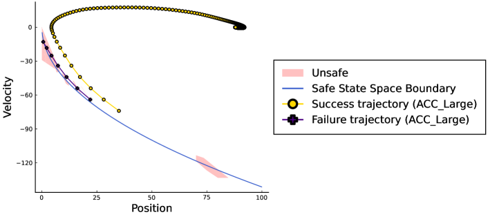
Figure 5: This plot shows the (input) state space for the ACC_Large NNCS: The blue line represents the boundary of the safe state space; the red areas indicate regions with counterexamples; the indigo and yellow line show potential trajectories of the system (dots represent discrete controller decisions).

Information on runtimes.

The runtimes can be seen in Table 4 where #Filtered corresponds to the number of counterexample regions that were found to be spurious. The approximation reduces the runtime for larger networks. This is the case because the overapproximate constraints can filter out numerous counterexample regions, which would otherwise have to be processed by the Filter procedure. This effect is less significant for smaller networks where the time for overapproximation construction takes longer in comparison to the NN analysis time. Preliminary experiments on ACC_Large where we soundly omitted all approximations of nonlinear constraints led to the generation of over 20,000 spurious counterexample regions that had to be filtered through SMT queries at a significant performance cost.

Table 4: Runtime of SNNT on the ACC networks per approximation. Final column lists filtered counterexamples for ACC_Large

Approx.	ACC	ACC_Large	ACC_Large retrained	#Filtered
$N=1$	56s	181s	98s	1780
$N=2$	53s	173s	70s	1859
$N=3$	96s	144s	83s	1179

Appendix 0.F Comparison to other tools

Approximation Scheme employed for NNV.

We consider input space stripes of width $\sigma>0$, i.e. $\left(p_{rel},v_{rel}\right)\in\left[p_{0},p_{0}+\sigma\right]\times\left[-\sqrt{2Ap_{rel}}+\epsilon,\frac{TB}{2}\right]$ ($v_{rel}$ is bounded through the minimally allowed velocity and the maximal velocity that can still decrease $p_{rel}$). While $\sigma$ determines the granularity of the under-approximation of NN inputs, $\epsilon>0$ discards velocities too close to the loop invariant which cannot be proven using an underapproximation and must be non-zero to prove any system. For each stripe we compute the smallest reachable position $p^{*}$ and compute a piece-wise linear overapproximation of the negated loop invariant $p_{rel}<v_{rel}^{2}/\left(2A\right)$ on the interval $\left[p^{*},p_{0}\right]$ using an approach conceptually similar to OVERT [57]. We determine the number of pieces through a step size $\rho>0$, i.e. the interval $\left[p^{*},p^{*}+\rho\right]$ will have a different line segment than the interval $\left[p^{*}+\rho,p^{*}+2\rho\right]$. As the negation of the loop invariant (the blue line in Figure 5) is non-convex, we integrated an iterative check for disjunctions of unsafe sets into the verification procedure of NNV.

Comparison with SMT solvers.

An alternative approach for the verification of non-linear OLNNV queries could be encoding the problem using an off-the-shelf SMT solver. In this case, the SMT solver has to check the satisfiability of the nonlinear Equation 8. We can instrument the Lantern package [24] to encode the NN into a SMT formula. Thus, we performed a comparison on the ACC_Large NN as well as the retrained ACC_Large NN, i.e. on a satisfiable as well as a non-satisfiable instance. We compared our approach to Z3 [45], MathSAT [16] (due to its use of incremental linearization) as well as the first and second place of SMT-Comp 2023 in the QF_NRA track: Z3++ [15] and cvc5 [6]. The results of our comparison can be observed in Table 5. The observed timeouts after 12 hours are unsurprising insofar as the work on linear OLNNV techniques was partially motivated by the observation that classical SMT solvers struggle with the verification of NN.

Tool	ACC_Large		ACC_Large retrained
	Status	Time	Status	Time
Z3	unknown	2510s	unknown	1793s
Z3++	unknown	2550s	unknown	2269s
cvc5	TO	—	TO	—
MathSAT	TO	—	TO	—
SNNT	sat	2573s	unsat	1770s

Table 5: Comparison of SNNT with State-of-the-Art SMT solvers: Timeout (TO) was set to 12 hours

Comparison to the techniques by Genin et al. [24]

While the work by Genin et al. [24] represents a case-study with techniques specifically applied to an NN for a simplified airborne collision avoidance setting, some ideas from the example in [24] might in principle generalize to other case studies. Unfortunately, the case-study considered by [24] are not the NN from Julian et al. [35, 37], but simplified NN with a single acceleration control output. As the authors did not publish their trained NNs, their exact verification formulas, or their verification runtimes, we instead compare our approach with this line of work on our ACC benchmark. To this end, we approximate the verification property derived in Section 5.1 using the box approximation techniques described by the authors and use their Lantern Python package to translate the verification tasks into linear arithmetic SMT problems. Using Z3, their technique does not terminate within more than 50 hours on the (unsafe) ACC_Large network and thus fails to analyze the NN. This demonstrates significant scalability limitations compared to our approach. Moreover, it is worth pointing out that the authors themselves acknowledge that the technique is incomplete which distinguishes our complete lifting procedure from their approach.

Appendix 0.G Zeppelin Steering

As a further case study, we considered the task of steering a Zeppelin under uncertainty: The model’s goal was to learn avoiding obstacles while flying in a wind field with nondeterministic wind turbulences. This problem has previously been studied with differential hybrid games [51]. The examined scenario serves two purposes: On the one hand, it shows that our approach can reuse safety results from the dL literature which drastically increases its applicability; on the other hand it is a good illustration for why verification (rather than empirical evidence) is so important when deploying NN in safety-critical fields.

After transferring the differential hybrid games logic contract into a differential dynamic logic contract and proving its safety, we trained a model to avoid obstacles while flying in a wind field with uniformly random turbulences via PPO. After 1.4 million training steps, we obtained an agent that did not crash for an evaluation run of 30,000 time steps. Given these promising results we proceeded to verify the agent’s policy assuming a safe – or at least “almost safe” – flight strategy had been learnt. However, upon verifying the NN’s behavior for obstacles of circumfence 40, we found that it produced potentially unsafe actions for large parts of the input space. The reason this unsafety was not observable during empirical evaluation was the choice of uniformly random wind turbulences: The unsafe behavior only appears for specific sequences of turbulences which occur extremely rarely in the empirical setting. This flaw in the training methodology was only found due to the verification. This is where our approach differs from simulation-based evaluation: With an SMT filter timeout of 4 seconds, SNNT was able to provide an exhaustive characterization of all potentially unsafe regions in 2.07 hours while providing 256 concrete counterexample regions. Mosaic and OLNNV only take about 644 seconds leaving the bottlenecks at approximation construction (1794 seconds) and SMT based counterexample filtering (1.39 hours). This case study and the stark difference between simulation and verification underscore the importance of rigorous verification of NN as an addition to empirical evidence in safety-critical areas.

Appendix 0.H NMAC produced by NN-based ACASX advisories

Further counterexamples for the advisories of the NNCS can be found in Figures 6, 7, 8, 9 and 10. Counterexamples to the safety of NNCS advisories for non-level flight of the intruder in the case of a previous advisory Do Not Climb and Do Not Descend can be found in Figures 11 and 12. Note, that there exist two interpretations of advisories where one advises on relative velocity while the other advises on absolute velocity. The counterexamples in Figures 11 and 12 opt for the relative velocity interpretation of advisories.

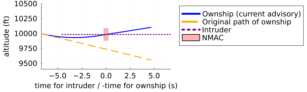
Figure 6: After a previous advisory to descent at least 1500ft/min, the NN advises the pilot to strengthen climb to at least 1500ft/min leading to a NMAC.

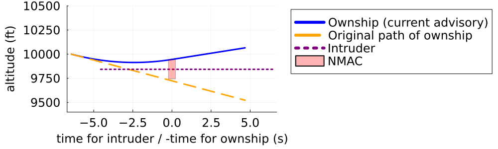
Figure 7: After a previous advisory to strengthen descent to at least 1500ft/min, the NN advises the pilot to strengthen climb to at least 1500ft/min leading to a NMAC.

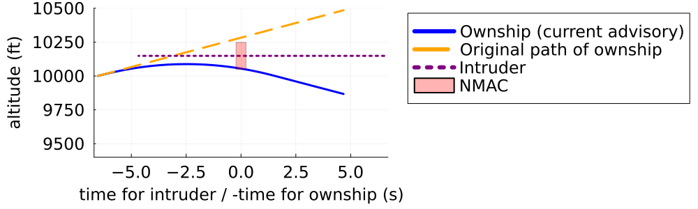
Figure 8: After a previous advisory to strengthen climb to at least 1500ft/min, the NN advises the pilot to strengthen descent to at least 2500ft/min leading to a NMAC.

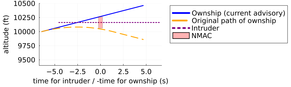
Figure 9: After a previous advisory to strengthen descent to at least 2500ft/min, the NN advises the pilot to strengthen descent to at least 2500ft/min leading to a NMAC.

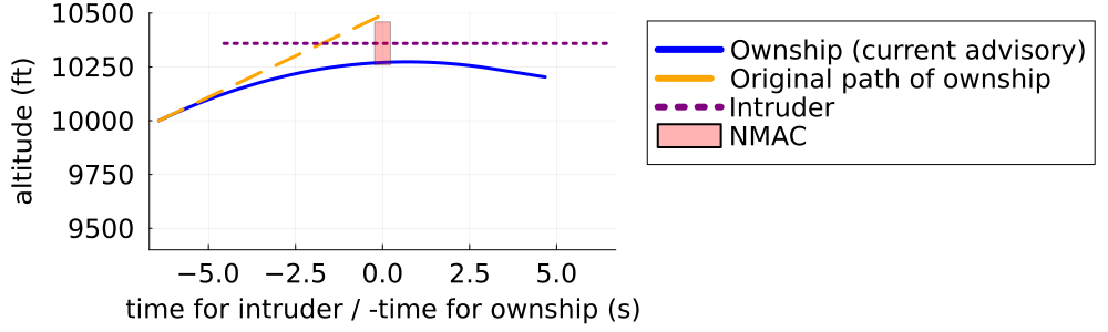
Figure 10: After a previous advisory to strengthen climb to at least 2500ft/min, the NN advises the pilot to strengthen descent to at least 1500ft/min leading to a NMAC.

Figure 11: After a previous advisory to not climb, the NN advises the pilot to climb with at least 1500ft/min leading to a NMAC.

Figure 12: After a previous advisory to not descend, the NN advises the pilot to descend with at least 1500ft/min leading to a NMAC.

References

- [1] Akintunde, M.E., Botoeva, E., Kouvaros, P., Lomuscio, A.: Formal verification of neural agents in non-deterministic environments. Auton. Agents Multi Agent Syst. 36(1), 6 (2022). https://doi.org/10.1007/s10458-021-09529-3
- [2] Althoff, M.: An introduction to CORA 2015. In: Frehse, G., Althoff, M. (eds.) ARCH14-15. 1st and 2nd International Workshop on Applied veRification for Continuous and Hybrid Systems. EPiC Series in Computing, vol. 34, pp. 120–151. EasyChair (2015). https://doi.org/10.29007/zbkv
- [3] Bak, S.: nnenum: Verification of ReLU neural networks with optimized abstraction refinement. In: Dutle, A., Moscato, M.M., Titolo, L., Muñoz, C.A., Perez, I. (eds.) NASA Formal Methods - 13th International Symposium, NFM 2021, Virtual Event, May 24-28, 2021, Proceedings. LNCS, vol. 12673, pp. 19–36. Springer (2021). https://doi.org/10.1007/978-3-030-76384-8_2
- [4] Bak, S., Tran, H.: Neural network compression of ACAS Xu early prototype is unsafe: Closed-loop verification through quantized state backreachability. In: Deshmukh, J.V., Havelund, K., Perez, I. (eds.) NASA Formal Methods - 14th International Symposium, NFM 2022, Pasadena, CA, USA, May 24-27, 2022, Proceedings. LNCS, vol. 13260, pp. 280–298. Springer (2022). https://doi.org/10.1007/978-3-031-06773-0_15
- [5] Bak, S., Tran, H., Hobbs, K., Johnson, T.T.: Improved geometric path enumeration for verifying ReLU neural networks. In: Lahiri, S.K., Wang, C. (eds.) Computer Aided Verification - 32nd International Conference, CAV 2020, Los Angeles, CA, USA, July 21-24, 2020, Proceedings, Part I. LNCS, vol. 12224, pp. 66–96. Springer (2020). https://doi.org/10.1007/978-3-030-53288-8_4
- [6] Barbosa, H., Barrett, C.W., Brain, M., Kremer, G., Lachnitt, H., Mann, M., Mohamed, A., Mohamed, M., Niemetz, A., Nötzli, A., Ozdemir, A., Preiner, M., Reynolds, A., Sheng, Y., Tinelli, C., Zohar, Y.: cvc5: A versatile and industrial-strength SMT solver. In: Fisman, D., Rosu, G. (eds.) Tools and Algorithms for the Construction and Analysis of Systems - 28th International Conference, TACAS 2022, Held as Part of the European Joint Conferences on Theory and Practice of Software, ETAPS 2022, Munich, Germany, April 2-7, 2022, Proceedings, Part I. LNCS, vol. 13243, pp. 415–442. Springer (2022). https://doi.org/10.1007/978-3-030-99524-9_24
- [7] Barrett, C., Katz, G., Guidotti, D., Pulina, L., Narodytska, N., Tacchella, A.: The VNNLIB standard for benchmarks (draft). Tech. rep., AIMS-LAB, University of Genoa (2021)
- [8] Bezanson, J., Edelman, A., Karpinski, S., Shah, V.B.: Julia: A fresh approach to numerical computing. SIAM Review 59(1), 65–98 (9 2017). https://doi.org/10.1137/141000671
- [9] Biere, A.: PicoSAT essentials. J. Satisf. Boolean Model. Comput. 4(2-4), 75–97 (2008). https://doi.org/10.3233/sat190039
- [10] Bogomolov, S., Forets, M., Frehse, G., Potomkin, K., Schilling, C.: JuliaReach: a toolbox for set-based reachability. In: Ozay, N., Prabhakar, P. (eds.) Proceedings of the 22nd ACM International Conference on Hybrid Systems: Computation and Control, HSCC 2019, Montreal, QC, Canada, April 16-18, 2019. pp. 39–44. ACM (2019). https://doi.org/10.1145/3302504.3311804
- [11] Bolewski, J., Lucibello, C., Bouton, M.: PicoSAT.jl (2020), https://github.com/sisl/PicoSAT.jl
- [12] Brix, C., Müller, M.N., Bak, S., Johnson, T.T., Liu, C.: First three years of the international verification of neural networks competition (VNN-COMP). Int. J. Softw. Tools Technol. Transf. 25(3), 329–339 (2023). https://doi.org/10.1007/s10009-023-00703-4
- [13] Brosowsky, M., Keck, F., Ketterer, J., Isele, S., Slieter, D., Zöllner, M.: Safe deep reinforcement learning for adaptive cruise control by imposing state-specific safe sets. In: 2021 IEEE Intelligent Vehicles Symposium (IV). pp. 488–495 (2021). https://doi.org/10.1109/IV48863.2021.9575258
- [14] Bunel, R., Lu, J., Turkaslan, I., Torr, P.H.S., Kohli, P., Kumar, M.P.: Branch and bound for piecewise linear neural network verification. J. Mach. Learn. Res. 21, 42:1–42:39 (2020)
- [15] Cai, S., Li, B., Zhang, X.: Local search for SMT on linear integer arithmetic. In: Shoham, S., Vizel, Y. (eds.) Computer Aided Verification - 34th International Conference, CAV 2022, Haifa, Israel, August 7-10, 2022, Proceedings, Part II. Lecture Notes in Computer Science, vol. 13372, pp. 227–248. Springer (2022). https://doi.org/10.1007/978-3-031-13188-2_12
- [16] Cimatti, A., Griggio, A., Schaafsma, B.J., Sebastiani, R.: The mathsat5 SMT solver. In: Piterman, N., Smolka, S.A. (eds.) Tools and Algorithms for the Construction and Analysis of Systems - 19th International Conference, TACAS 2013, Held as Part of the European Joint Conferences on Theory and Practice of Software, ETAPS 2013, Rome, Italy, March 16-24, 2013. Proceedings. Lecture Notes in Computer Science, vol. 7795, pp. 93–107. Springer (2013). https://doi.org/10.1007/978-3-642-36742-7_7
- [17] Daggitt, M.L., Kokke, W., Atkey, R., Arnaboldi, L., Komendantskaya, E.: Vehicle: Interfacing neural network verifiers with interactive theorem provers. CoRR abs/2202.05207 (2022)
- [18] Dutta, S., Chen, X., Sankaranarayanan, S.: Reachability analysis for neural feedback systems using regressive polynomial rule inference. In: Ozay, N., Prabhakar, P. (eds.) Proceedings of the 22nd ACM International Conference on Hybrid Systems: Computation and Control, HSCC 2019, Montreal, QC, Canada, April 16-18, 2019. pp. 157–168. ACM (2019). https://doi.org/10.1145/3302504.3311807
- [19] Eleftheriadis, C., Kekatos, N., Katsaros, P., Tripakis, S.: On neural network equivalence checking using SMT solvers. In: Bogomolov, S., Parker, D. (eds.) Formal Modeling and Analysis of Timed Systems - 20th International Conference, FORMATS 2022, Warsaw, Poland, September 13-15, 2022, Proceedings. LNCS, vol. 13465, pp. 237–257. Springer (2022). https://doi.org/10.1007/978-3-031-15839-1_14
- [20] Fan, J., Huang, C., Chen, X., Li, W., Zhu, Q.: ReachNN*: A tool for reachability analysis of neural-network controlled systems. In: Hung, D.V., Sokolsky, O. (eds.) Automated Technology for Verification and Analysis - 18th International Symposium, ATVA 2020, Hanoi, Vietnam, October 19-23, 2020, Proceedings. LNCS, vol. 12302, pp. 537–542. Springer (2020). https://doi.org/10.1007/978-3-030-59152-6_30
- [21] Fulton, N., Mitsch, S., Quesel, J., Völp, M., Platzer, A.: KeYmaera X: an axiomatic tactical theorem prover for hybrid systems. In: Felty, A.P., Middeldorp, A. (eds.) Automated Deduction - CADE-25 - 25th International Conference on Automated Deduction, Berlin, Germany, August 1-7, 2015, Proceedings. LNCS, vol. 9195, pp. 527–538. Springer (2015). https://doi.org/10.1007/978-3-319-21401-6_36
- [22] Fulton, N., Platzer, A.: Safe reinforcement learning via formal methods: Toward safe control through proof and learning. In: McIlraith, S.A., Weinberger, K.Q. (eds.) Proceedings of the Thirty-Second AAAI Conference on Artificial Intelligence, (AAAI-18), New Orleans, Louisiana, USA, February 2-7, 2018. pp. 6485–6492. AAAI Press (2018). https://doi.org/10.1609/aaai.v32i1.12107
- [23] Ganzinger, H., Hagen, G., Nieuwenhuis, R., Oliveras, A., Tinelli, C.: DPLL(T): fast decision procedures. In: Alur, R., Peled, D.A. (eds.) Computer Aided Verification, 16th International Conference, CAV 2004, Boston, MA, USA, July 13-17, 2004, Proceedings. LNCS, vol. 3114, pp. 175–188. Springer (2004). https://doi.org/10.1007/978-3-540-27813-9_14
- [24] Genin, D., Papusha, I., Brulé, J., Young, T., Mullins, G.E., Kouskoulas, Y., Wu, R., Schmidt, A.C.: Formal verification of neural network controllers for collision-free flight. In: Bloem, R., Dimitrova, R., Fan, C., Sharygina, N. (eds.) Software Verification - 13th International Conference, VSTTE 2021, New Haven, CT, USA, October 18-19, 2021, and 14th International Workshop, NSV 2021, Los Angeles, CA, USA, July 18-19, 2021, Revised Selected Papers. LNCS, vol. 13124, pp. 147–164. Springer (2021). https://doi.org/10.1007/978-3-030-95561-8_9
- [25] Grundt, D., Jurj, S.L., Hagemann, W., Kröger, P., Fränzle, M.: Verification of sigmoidal artificial neural networks using iSAT. In: Proceedings The 7h International Workshop on Symbolic-Numeric Methods for Reasoning about CPS and IoT. vol. 361, pp. 45–60. Electronic Proceedings in Theoretical Computer Science (2021). https://doi.org/10.4204/EPTCS.361.6
- [26] Henriksen, P., Lomuscio, A.: DEEPSPLIT: an efficient splitting method for neural network verification via indirect effect analysis. In: Zhou, Z. (ed.) Proceedings of the Thirtieth International Joint Conference on Artificial Intelligence, IJCAI 2021, Virtual Event / Montreal, Canada, 19-27 August 2021. pp. 2549–2555. ijcai.org (2021). https://doi.org/10.24963/ijcai.2021/351
- [27] Henriksen, P., Lomuscio, A.R.: Efficient neural network verification via adaptive refinement and adversarial search. In: Giacomo, G.D., Catalá, A., Dilkina, B., Milano, M., Barro, S., Bugarín, A., Lang, J. (eds.) ECAI 2020 - 24th European Conference on Artificial Intelligence, 29 August-8 September 2020, Santiago de Compostela, Spain, August 29 - September 8, 2020. Frontiers in Artificial Intelligence and Applications, vol. 325, pp. 2513–2520. IOS Press (2020). https://doi.org/10.3233/FAIA200385
- [28] Huang, C., Fan, J., Chen, X., Li, W., Zhu, Q.: POLAR: A polynomial arithmetic framework for verifying neural-network controlled systems. In: Bouajjani, A., Holík, L., Wu, Z. (eds.) Automated Technology for Verification and Analysis - 20th International Symposium, ATVA 2022, Virtual Event, October 25-28, 2022, Proceedings. LNCS, vol. 13505, pp. 414–430. Springer (2022). https://doi.org/10.1007/978-3-031-19992-9_27
- [29] Huang, C., Fan, J., Li, W., Chen, X., Zhu, Q.: ReachNN: Reachability analysis of neural-network controlled systems. ACM Trans. Embed. Comput. Syst. 18(5s), 106:1–106:22 (2019). https://doi.org/10.1145/3358228
- [30] Ivanov, R., Carpenter, T.J., Weimer, J., Alur, R., Pappas, G.J., Lee, I.: Verifying the safety of autonomous systems with neural network controllers. ACM Trans. Embed. Comput. Syst. 20(1), 7:1–7:26 (2021). https://doi.org/10.1145/3419742
- [31] Ivanov, R., Carpenter, T.J., Weimer, J., Alur, R., Pappas, G.J., Lee, I.: Verisig 2.0: Verification of neural network controllers using Taylor model preconditioning. In: Silva, A., Leino, K.R.M. (eds.) Computer Aided Verification - 33rd International Conference, CAV 2021, Virtual Event, July 20-23, 2021, Proceedings, Part I. LNCS, vol. 12759, pp. 249–262. Springer (2021). https://doi.org/10.1007/978-3-030-81685-8_11
- [32] Jeannin, J., Ghorbal, K., Kouskoulas, Y., Schmidt, A.C., Gardner, R.W., Mitsch, S., Platzer, A.: A formally verified hybrid system for safe advisories in the next-generation airborne collision avoidance system. Int. J. Softw. Tools Technol. Transf. 19(6), 717–741 (2017). https://doi.org/10.1007/s10009-016-0434-1
- [33] Johnson, T.T., Lopez, D.M., Benet, L., Forets, M., Guadalupe, S., Schilling, C., Ivanov, R., Carpenter, T.J., Weimer, J., Lee, I.: ARCH-COMP21 category report: Artificial intelligence and neural network control systems (AINNCS) for continuous and hybrid systems plants. In: Frehse, G., Althoff, M. (eds.) 8th International Workshop on Applied Verification of Continuous and Hybrid Systems (ARCH21), Brussels, Belgium, July 9, 2021. EPiC Series in Computing, vol. 80, pp. 90–119. EasyChair (2021). https://doi.org/10.29007/kfk9
- [34] Jovanovic, D., de Moura, L.: Solving non-linear arithmetic. ACM Commun. Comput. Algebra 46(3/4), 104–105 (2012). https://doi.org/10.1145/2429135.2429155
- [35] Julian, K.D., Lopez, J., Brush, J.S., Owen, M.P., Kochenderfer, M.J.: Policy compression for aircraft collision avoidance systems. In: 2016 IEEE/AIAA 35th Digital Avionics Systems Conference (DASC). pp. 1–10 (2016). https://doi.org/10.1109/DASC.2016.7778091
- [36] Julian, K.D., Sharma, S., Jeannin, J.B., Kochenderfer, M.J.: Verifying aircraft collision avoidance neural networks through linear approximations of safe regions. In: Verification of Neural Networks (VNN 2019) (2019). https://doi.org/10.48550/arXiv.1903.00762
- [37] Julian, K.D.: Safe and efficient aircraft guidance and control using neural networks. Ph.D. thesis, Stanford University (2020)
- [38] Katz, G., Barrett, C.W., Dill, D.L., Julian, K., Kochenderfer, M.J.: Reluplex: An efficient SMT solver for verifying deep neural networks. In: Majumdar, R., Kuncak, V. (eds.) Computer Aided Verification - 29th International Conference, CAV 2017, Heidelberg, Germany, July 24-28, 2017, Proceedings, Part I. LNCS, vol. 10426, pp. 97–117. Springer (2017). https://doi.org/10.1007/978-3-319-63387-9_5
- [39] Katz, G., Huang, D.A., Ibeling, D., Julian, K., Lazarus, C., Lim, R., Shah, P., Thakoor, S., Wu, H., Zeljic, A., Dill, D.L., Kochenderfer, M.J., Barrett, C.W.: The Marabou framework for verification and analysis of deep neural networks. In: Dillig, I., Tasiran, S. (eds.) Computer Aided Verification - 31st International Conference, CAV 2019, New York City, NY, USA, July 15-18, 2019, Proceedings, Part I. LNCS, vol. 11561, pp. 443–452. Springer (2019). https://doi.org/10.1007/978-3-030-25540-4_26
- [40] Könighofer, B., Bloem, R., Ehlers, R., Pek, C.: Correct-by-construction runtime enforcement in AI - A survey. In: Principles of Systems Design - Essays Dedicated to Thomas A. Henzinger on the Occasion of His 60th Birthday. pp. 650–663 (2022). https://doi.org/10.1007/978-3-031-22337-2_31
- [41] Lechner, M., Zikelic, D., Chatterjee, K., Henzinger, T.A.: Infinite time horizon safety of Bayesian neural networks. In: Ranzato, M., Beygelzimer, A., Dauphin, Y.N., Liang, P., Vaughan, J.W. (eds.) Advances in Neural Information Processing Systems 34: Annual Conference on Neural Information Processing Systems 2021, NeurIPS 2021, December 6-14, 2021, virtual. pp. 10171–10185 (2021)
- [42] Loos, S.M., Platzer, A.: Differential refinement logic. In: Grohe, M., Koskinen, E., Shankar, N. (eds.) Proceedings of the 31st Annual ACM/IEEE Symposium on Logic in Computer Science, LICS ’16, New York, NY, USA, July 5-8, 2016. pp. 505–514. ACM (2016). https://doi.org/10.1145/2933575.2934555
- [43] Lopez, D.M., Althoff, M., Benet, L., Chen, X., Fan, J., Forets, M., Huang, C., Johnson, T.T., Ladner, T., Li, W., et al.: ARCH-COMP22 category report: Artificial intelligence and neural network control systems (AINNCS) for continuous and hybrid systems plants. In: Proceedings of 9th International Workshop on Applied. vol. 90, pp. 142–184 (2022). https://doi.org/10.29007/wfgr
- [44] Mitsch, S., Platzer, A.: ModelPlex: verified runtime validation of verified cyber-physical system models. Formal Methods Syst. Des. 49(1-2), 33–74 (2016). https://doi.org/10.1007/s10703-016-0241-z
- [45] de Moura, L.M., Bjørner, N.S.: Z3: an efficient SMT solver. In: Ramakrishnan, C.R., Rehof, J. (eds.) Tools and Algorithms for the Construction and Analysis of Systems, 14th International Conference, TACAS 2008, Held as Part of the Joint European Conferences on Theory and Practice of Software, ETAPS 2008, Budapest, Hungary, March 29-April 6, 2008. Proceedings. LNCS, vol. 4963, pp. 337–340. Springer (2008). https://doi.org/10.1007/978-3-540-78800-3_24
- [46] Olson, W.A.: Airborne collision avoidance system X. Tech. rep., Massachusetts Institute of Technology Lexington Lincoln Lab (2015)
- [47] Papusha, I., Wu, R., Brulé, J., Kouskoulas, Y., Genin, D., Schmidt, A.: Incorrect by Construction: Fine Tuning Neural Networks for Guaranteed Performance on Finite Sets of Examples. In: 3rd Workshop on Formal Methods for ML-Enabled Autonomous Systems (FOMLAS). pp. 1–12 (2020). https://doi.org/10.48550/arXiv.2008.01204
- [48] Platzer, A.: Differential dynamic logic for hybrid systems. J. Autom. Reason. 41(2), 143–189 (2008). https://doi.org/10.1007/s10817-008-9103-8
- [49] Platzer, A.: The complete proof theory of hybrid systems. In: Proceedings of the 27th Annual IEEE Symposium on Logic in Computer Science, LICS 2012, Dubrovnik, Croatia, June 25-28, 2012. pp. 541–550. IEEE Computer Society (2012). https://doi.org/10.1109/LICS.2012.64
- [50] Platzer, A.: A complete uniform substitution calculus for differential dynamic logic. J. Autom. Reason. 59(2), 219–265 (2017). https://doi.org/10.1007/s10817-016-9385-1
- [51] Platzer, A.: Differential hybrid games. ACM Trans. Comput. Log. 18(3), 19:1–19:44 (2017). https://doi.org/10.1145/3091123
- [52] Platzer, A., Tan, Y.K.: Differential equation invariance axiomatization. J. ACM 67(1), 6:1–6:66 (2020). https://doi.org/10.1145/3380825
- [53] Qin, C., Dvijotham, K.D., O’Donoghue, B., Bunel, R., Stanforth, R., Gowal, S., Uesato, J., Swirszcz, G., Kohli, P.: Verification of non-linear specifications for neural networks. In: 7th International Conference on Learning Representations, ICLR 2019, New Orleans, LA, USA, May 6-9, 2019 (2019)
- [54] Raffin, A., Hill, A., Gleave, A., Kanervisto, A., Ernestus, M., Dormann, N.: Stable-baselines3: Reliable reinforcement learning implementations. J. Mach. Learn. Res. 22, 268:1–268:8 (2021)
- [55] Schilling, C., Forets, M., Guadalupe, S.: Verification of neural-network control systems by integrating Taylor models and zonotopes. CoRR abs/2112.09197 (2021)
- [56] Shriver, D., Elbaum, S.G., Dwyer, M.B.: DNNV: A framework for deep neural network verification. In: Silva, A., Leino, K.R.M. (eds.) Computer Aided Verification - 33rd International Conference, CAV 2021, Virtual Event, July 20-23, 2021, Proceedings, Part I. LNCS, vol. 12759, pp. 137–150. Springer (2021). https://doi.org/10.1007/978-3-030-81685-8_6
- [57] Sidrane, C., Maleki, A., Irfan, A., Kochenderfer, M.J.: OVERT: an algorithm for safety verification of neural network control policies for nonlinear systems. Journal of Machine Learning Research 23(117), 1–45 (2022)
- [58] Sogokon, A., Mitsch, S., Tan, Y.K., Cordwell, K., Platzer, A.: Pegasus: Sound continuous invariant generation. Form. Methods Syst. Des. 58(1), 5–41 (2022). https://doi.org/10.1007/s10703-020-00355-z, special issue for selected papers from FM’19
- [59] Tarski, A.: A Decision Method for Elementary Algebra and Geometry. University of California Press, Berkeley and Los Angeles (1951)
- [60] Tran, H., Lopez, D.M., Musau, P., Yang, X., Nguyen, L.V., Xiang, W., Johnson, T.T.: Star-based reachability analysis of deep neural networks. In: ter Beek, M.H., McIver, A., Oliveira, J.N. (eds.) Formal Methods - The Next 30 Years - Third World Congress, FM 2019, Porto, Portugal, October 7-11, 2019, Proceedings. LNCS, vol. 11800, pp. 670–686. Springer (2019). https://doi.org/10.1007/978-3-030-30942-8_39
- [61] Tran, H., Yang, X., Lopez, D.M., Musau, P., Nguyen, L.V., Xiang, W., Bak, S., Johnson, T.T.: NNV: the neural network verification tool for deep neural networks and learning-enabled cyber-physical systems. In: Lahiri, S.K., Wang, C. (eds.) Computer Aided Verification - 32nd International Conference, CAV 2020, Los Angeles, CA, USA, July 21-24, 2020, Proceedings, Part I. LNCS, vol. 12224, pp. 3–17. Springer (2020). https://doi.org/10.1007/978-3-030-53288-8_1
- [62] Wang, S., Pei, K., Whitehouse, J., Yang, J., Jana, S.: Efficient formal safety analysis of neural networks. In: Bengio, S., Wallach, H.M., Larochelle, H., Grauman, K., Cesa-Bianchi, N., Garnett, R. (eds.) Advances in Neural Information Processing Systems 31: Annual Conference on Neural Information Processing Systems 2018, NeurIPS 2018, December 3-8, 2018, Montréal, Canada. pp. 6369–6379 (2018)
- [63] Wang, S., Zhang, H., Xu, K., Lin, X., Jana, S., Hsieh, C., Kolter, J.Z.: Beta-crown: Efficient bound propagation with per-neuron split constraints for neural network robustness verification. In: Ranzato, M., Beygelzimer, A., Dauphin, Y.N., Liang, P., Vaughan, J.W. (eds.) Advances in Neural Information Processing Systems 34: Annual Conference on Neural Information Processing Systems 2021, NeurIPS 2021, December 6-14, 2021, virtual. pp. 29909–29921 (2021)
- [64] Xiang, W., Tran, H., Yang, X., Johnson, T.T.: Reachable set estimation for neural network control systems: A simulation-guided approach. IEEE Trans. Neural Networks Learn. Syst. 32(5), 1821–1830 (2021). https://doi.org/10.1109/TNNLS.2020.2991090
- [65] Xu, K., Shi, Z., Zhang, H., Wang, Y., Chang, K., Huang, M., Kailkhura, B., Lin, X., Hsieh, C.: Automatic perturbation analysis for scalable certified robustness and beyond. In: Larochelle, H., Ranzato, M., Hadsell, R., Balcan, M., Lin, H. (eds.) Advances in Neural Information Processing Systems 33: Annual Conference on Neural Information Processing Systems 2020, NeurIPS 2020, December 6-12, 2020, virtual (2020)
- [66] Xu, K., Zhang, H., Wang, S., Wang, Y., Jana, S., Lin, X., Hsieh, C.: Fast and complete: Enabling complete neural network verification with rapid and massively parallel incomplete verifiers. In: 9th International Conference on Learning Representations, ICLR 2021, Virtual Event, Austria, May 3-7, 2021 (2021)
- [67] Zhang, H., Weng, T., Chen, P., Hsieh, C., Daniel, L.: Efficient neural network robustness certification with general activation functions. In: Bengio, S., Wallach, H.M., Larochelle, H., Grauman, K., Cesa-Bianchi, N., Garnett, R. (eds.) Advances in Neural Information Processing Systems 31: Annual Conference on Neural Information Processing Systems 2018, NeurIPS 2018, December 3-8, 2018, Montréal, Canada. pp. 4944–4953 (2018)