Recovering the Fragmentation Rate in the Growth-Fragmentation Equation
Abstract
We consider the inverse problem of determining the fragmentation rate from noisy measurements in the growth-fragmentation equation. We use Fourier transform theory on locally compact groups to treat this problem for general fragmentation probabilities. We develop a regularization method based on spectral filtering, which allows us to deal with the inverse problem in weighted spaces. As a result, we obtain a regularization method with error of order , where is the noise level and is the a priori regularity order of the fragmentation rate.
-
February 2022
Keywords: Size-structured models; Regularization techniques; Fourier transform on groups; growth-fragmentation equation; mathematical biology models.
1 Introduction
Growth-fragmentation equations describe, in a quantitative way, the evolution process of the density of an ensemble of particles that divide according to a certain fragmentation rate. In other words, we assume that each particle grows over time, and splits into smaller particles, in such a way that the total mass is conserved. This model is used in biological phenomena for instance, in cell division processes [1, 2, 3, 4] and protein polymerization [5]. It also appears in telecommunications [6]. The goal of this article is to address the inverse problem for a class of such equations making use of the asymptotic behavior of their solutions which in turn, after proper scaling, converge to a stable distribution in time [1, 7, 8].
The growth-fragmentation equation considered here can be expressed using the following integro-differential equation,
| (1) |
where represents the density of particles of mass at time , with initial condition . The function is the growth rate for particles of mass . The function represents the conditional probability that a particle of mass splits into smaller particles of mass . The function is the fragmentation rate of particles of mass .
A natural question concerns to the asymptotic behaviour of the population density , when . In [7, 8], it is shown that under certain conditions on the coefficients , , and , there exists an unique eigenpair such that
| (2) |
Moreover, in appropriate weighted norms, we have that when the time goes to infinity.
Thus, we shall focus on the pair , which corresponds to the eigenpair of a linear operator [7]. They have the biophysical interpretation of the asymptotic distribution of the population density and the corresponding convergence rate. In principle, such quantities could be experimentally observed in some situations due to the exponential decay rate. This was used for instance in [9]. The function alluded to above is the stable distribution which is observed in a broad class of structured population models [1]. The importance of studying instead of is that the variable is removed, which reduces the study of a two-dimensional problem to a one-dimensional.
We are interested in how to recover in a stable way the fragmentation rate from noisy measurements of and . Our strategy is to study rather than , as proposed in [10, 11], and then use truncated division by to recover . Thus, the inverse problem under consideration is how to recover in a stable way from approximate knowledge of and , in which is the solution of
| (3) |
where
| (4) |
In [10, 12, 9] the inverse problem was treated for the equal mitosis case, that is, when a particle splits into two small particles with half of its mass. In this case, the parameters are
| (5) |
A more general class of conditional probability density kernels is given by the self-similar ones, that is, when
| (6) |
where is a probability measure in . Self-similar probabilities arise when the fragmentation depends on the ratio between the size of the mother particle and the size of the next-generation particle. The inverse problem for self-similar probabilities was treated in the works [11, 13].
The aim of the present work is to address this inverse problem for more general probabilities. Namely, we consider conditional probabilities of the form
| (7) |
where is an increasing diffeomorphism from to , and is a probability on . The transport operation is defined by
| (8) |
We shall denote conditional densities in (7) as transport probabilities. Observe that if we take the exponential function , then the transport operation for this function is the usual product on the positive real line. Hence, transport probabilities generalize self-similar probabilities.
We treat the inverse problem described in Eq. (3). Here, we do not require that the mass must be conserved in the division process. This is in order not to restrict this method only to biological models, and also to use it in real-world applications. treating this problem from a more general point of view. We do that in two steps. Firstly, we guarantee that under some assumptions in , there exists a unique solution of Eq. (3). To do that, we establish that on proper spaces the operator is an isomorphism. The second step is to guarantee the stability of the inverse problem. For that, we propose a new regularization method. This method is based on the implementation of the Fourier transform theory, and spectral filtering techniques.
We show that the Quasi-Reversibility approach [12] is a particular case of our method. Compared to regularization methods based on convolution [11, 13], our method improves the error order. Namely, we obtain an error of order , where is the noise level.
This article is organized as follows: in Section 2, we study the transport operation and some relations with the Fourier transform on locally compact abelian groups. In Section 3, we discuss the invertibility of the operator in proper spaces. In Section 4, we present a new regularization method to treat the stability of the inverse problem. In Section 5, we give examples for which some of the Hypotheses Eq. (3.1) or Eq. (4.1) are satisfied. Finally, in Section 6, we present the numerical implementation of our method.
2 Preliminaries
To fix the notation, we briefly review some concepts of Fourier transform for locally compact groups. We refer the reader to [14] for more details. We recall that the Haar measure on an abelian group is the unique non-negative and regular measure, up to a positive multiplicative constant, which is translation invariant. Here, by translation, we mean the action of multiplication by group elements.
We define the transport operation as
| (9) |
where is an increasing diffeomorphism from to . The pair equipped with the induced topology of is a locally compact group. Moreover, the Haar measure is given by the measure
| (10) |
where is the Lebesgue measure on the positive real line. In this context, we can develop the theory of the Fourier transform on the group .
2.1 Fourier transform on .
The Fourier transform on the group is defined for a function and a real number as
| (11) |
In this general context, the Fourier transform theory on can be developed in a similar fashion as in the standard case . In particular, we obtain the inversion and the Plancherel theorems. See [14] for more details.
Theorem (Inversion theorem [14]).
Suppose that and then for a.e positive number we have
| (12) |
Theorem (Plancherel Theorem [14]).
The Fourier transform , restricted to is an isometry onto a dense linear subspace of . Hence, it may be extended, in a unique manner, to an isometry from to
2.2 The spaces.
In order to extend the Plancherel theorem, we define the space. They are a natural generalization of the space. More precisely, the space is defined as Observe that there exists a canonical isomorphism between and which is given by
| (13) |
We now define the Fourier transform on as
| (14) |
Thus, by the Plancherel Theorem, the generalized Fourier transform is an isometry.
For the case when is a probability measure on satisfying
| (15) |
we define the Fourier transform of the probability by
| (16) |
for any real number
2.3 The Fourier transform and the convolution operator
We now consider the convolution-type operator induced by the probability and given by
| (17) |
In the same manner, as in the case of and under some conditions of integrability, the Fourier transform of a convolution operator becomes a multiplicative operator.
2.4 The Fourier transform of .
The Fourier transform on the real line has the property of diagonalizing differential operators. We now state an analogous version of this fact for the Fourier transform .
Proposition 2.1.
Suppose that belongs to the Sobolev space , and that the functions
| (19) |
are in . Then, we have
| (20) | ||||
Proof.
Using integration by parts, and the smoothness assumption of the function , we have that
Now, we observe that
and this proves our result. ∎
3 Invertibility of the operator .
Let be the operator defined as
| (21) |
We use the ideas of [11] in order to guarantee the invertibility of . We prove that under additional assumptions on the probability , the operator , has a bounded inverse in some subspaces of . If we apply the Fourier transform and the Eq. (18), we get that is in fact a multiplication operator
| (22) |
Thus, the operator has a bounded inverse on if the function
is bounded from below by positive constant on the real line. In some cases, the function never vanishes, but goes to zero when converges to or , in this situation, the function is bounded from below on compact sets of the real line. Moreover, for computational purposes, we are interested in a reconstruction on compact intervals. In this case, we focus on the invertibility of the operator on compact sets. To find a bounded inverse on an open set , we assume that the probability satisfies the following hypothesis.
Hypothesis 3.1.
There exists an open set such that the function is bounded from below by a positive constant on .
In Section 5 we give examples where the previous hypothesis is satisfied.
We consider the Paley-Wiener spaces , as the subspace of of all the functions whose Fourier transform has support on . Observe that if is on , then also lies on . Thus, the operator from to itself is well defined. Using the Fourier transform , and Eq. (18), we conclude the following proposition, which guarantees the existence of a bounded inverse.
Proposition 3.1.
Suppose that the probability satisfies Hypothesis 3.1, then the operator from to itself has a bounded inverse.
4 Regularization of the inverse problem
In this section, we discuss some methods to regularize the inverse problem, i.e, recover from noisy measurements of in some norm, in such a way that we can control the approximation error.
The main difficulty arises from the fact that we cannot estimate the norm of from . The principal idea in this section is to use the Fourier transform to turn the differential operator into a Fourier multiplication operator [15], and then, we regularize the inverse problem using spectral filters as described in [16].
4.1 Regularization by spectral filtering
We now present our strategy to regularize the inverse problem as follows. Using the Proposition 2.1, we see that under the Fourier transform, the differential operator is simply a quasi-multiplication operator, whose multiplication part is given by . Unfortunately, this function is unbounded in non-compact sets. Then, noisy data with small errors can approximate solutions with large errors, that is, it has a de-regularizing effect. To regularize the inverse problem, we define a multiplication approximation for , for which the multiplier is given by by a regularized filter . To be more precise, we define the approximation by
| (23) |
where
Let be a noisy measurement of in the product space , and let be the unique solution of Eq. (3) in . The following theorem gives error estimates for . It was inspired by [10], yet, the method is different because it focuses on regularizing the spectral signal of the differential operators.
Theorem 4.1 (Spectral regularization).
Let K be a subspace of . Suppose that there exists a positive constant , such that for all the bilinear operator defined from to is bounded. Assume that satisfies
where the constant does not depend on . Then, we have the estimate
Proof.
By the triangle inequality, we obtain
which implies the result. ∎
To apply the above result, we need to guarantee that for a fixed , the operator is well defined and bounded. For simplicity, we first consider the case when
| (24) |
and
| (25) |
are bounded functions on . To show that the operator is well defined, we consider the subspace of , which consists of all functions such that
are in . In that case, it is straightforward to show that the operator from to is well defined, and bounded. We use modified versions of Tikhonov and Landweber filters, to show that all the functions in Equation (25) are bounded. These filters are commonly used in regularization theory for compact operators [16].
4.2 Tikhonov filtering
In the classical case of linear operators, the solution to the problem , where is a non-negative linear and compact operator, can be regularized by using the filter
in the spectral variable. Indeed, considering the singular value decomposition of given by
the regularized solution to the problem is given by
See [16] for more details. For the problem under consideration, we modified the above function and consider the filter
| (26) |
We assume that the probability satisfies Hypothesis 3.1. Using these filters, we observe that the functions in Equation (25) are bounded with respect to the variable . Under these assumptions, the bilinear operator is bounded. In fact, a straightforward computation shows that
for some positive constant , which only depends on , , , .
We now state the following regularization method, based on the filter functions defined above.
Theorem 4.2 (Tikhonov regularization).
Assume that the probability satisfies Condition 15, and Hypothesis 3.1. Moreover, we assume that satisfies all the assumptions of Proposition 2.1, and
Then, for a noisy measurement of in the approximation using the filters Eq. (26) satisfies the estimate
for some positive constant which depends on , , , , and .
If satisfy , and
. Then, we can choose the optimal parameter to conclude
4.3 The quasi-reversibility Tikhonov filtering
The quasi-reversibility method proposed in [12] regularizes the inverse problem for the case of equal-mitosis. The idea of quasi-reversibility goes back to the work [17]. This method is based on adding a perturbation of a differential operator. In [13], an extension of this method was proposed for more general probabilities. We now present a different generalization using spectral filters. In fact, we show that there exists a relation between the quasi-reversibility method and our approach in the case of self-similar probabilities.
Let us first describe our method without going into technical details. For each real number , we defined the following modified Tikhonov filters
If the quotient factor blows up, then the last equation is not well defined. To avoid this kind of problem, we assume that the probability satisfies a stronger hypothesis than 3.1, namely, we assume that
Hypothesis 4.1.
There exist positive constants and such that for all and .
In Section 5, we give some examples for which the above hypothesis is satisfied. If we assume that is a smooth function satisfying Condition 29, we see that under the Fourier transform , the approximation in Eq. (23) solves the following differential equation
| (27) |
where
Thus, our method can be seen as a perturbation method [18]. For the self-similar case, that is, when , we see that
Taking , the perturbation method defined in Eq. (27) reduces to the quasi-reversibility method proposed in [13]. Using the same ideas of the proof of Theorem 4.2, we prove the next result.
Theorem 4.3 (Quasi-reversibility method).
Assume that the probability satisfies Eq. (15) and Hypothesis 4.1. Moreover, assume that satisfies all the assumptions of Proposition 2.1. If the functions
are in , then, for all noisy measurement of in the approximation satisfies the error estimate
for some constant which depends on , , , and .
If satisfies we can choose the regularization parameter , to conclude
4.4 The Landweber‘s method
Using the Tikhonov and quasi-reversibility filters, we obtain an approximation error of order . We improve this error order, and thus we obtain a better approximation. For that, we use a new filter, which is a modification of the classical Landweber filter
| (28) |
To implement these filters in Theorem 4.1, we first establish the following inequalities.
Lemma 4.1.
There exists a positive constant , such that for all and for all positive , the following estimate holds
where depends on , , , . Moreover, for all , such that , the following inequality holds
Proof.
Let us prove the first inequality. Using the change of variables , we see that
Since then applying the mean value inequality to the function , we obtain
thus as desired. To prove the second inequality, we observe that at the point , the function attains its maximum for . Thus, for all we have
∎
As a consequence of the previous lemma, we have that the functions in Eq. (25) are bounded. Thus, the bilinear operator is bounded. In fact, a straightforward computation shows that
for some positive constant , which only depends on , , , . Now, we apply Theorem 4.1 to the Landweber filter[16]. For that, we require a smoothness condition of order for the function
Theorem 4.4 (Landweber regularization).
Assume that the probability satisfies Eq. (15), and Hypothesis 3.1. Moreover, assume that , satisfies all the assumptions of Proposition 2.1, and the smoothness condition with order
Then, for all noisy measurement of in , the approximation defined in Eq. (23) using the spectral filter of Eq. (28) satisfies the error estimate
for some constant which depends on , , , , , and . Suppose that satisfies . We can choose the optimal parameter given by
which satisfies , to conclude
4.5 The unbounded case
In many cases, the functions in Equation (24) are not bounded. For instance, in the self-similar case. We now extend our results to the unbounded case. The idea is to regularize the functions in Equation (24) using a spectral filter. To do that, we write
and
where is the regularization parameter of the functions (24). Observe that the exponential decay guarantees that using in the place of , then the functions in Eq. (24) are bounded. Now, we show that if the function has fast decay, then the bounded function can be used to regularize the inverse problem, even if is not bounded.
Proposition 4.1.
Assume that the function satisfies
| (29) |
We define as the solution of Eq. (3), where the solution is associated with the function instead of . Then, we have that
where is a constant, which depends on the operator and the number .
Proof.
Observe that
Since
then, using the Fourier transform , we obtain
∎
5 Examples
To use the previous regularization methods, we need to verify that the probability satisfies Eq. (15), and some of the Hypotheses 3.1 or 4.1. In this section, we study some examples which satisfy the previous conditions. First, we discuss examples arising from the self-similar probabilities, that is, when and .
To check Hypothesis 4.1, it is sufficient to consider the case . In fact, if Hypothesis 4.1 holds for , then by triangle inequality we see that for all and
Thus, the Hypothesis 4.1 holds for all real numbers . We now study for which values of , and open sets , the Hypothesis 4.1 holds. Without loss of generality, we assume that .
5.1 The equal-mitosis
An important example of a self-similar case is the equal-mitosis. In equal-mitosis the conditional probability is given by . In this case, the Fourier transform of is given by
Thus, by the triangle inequality
| (30) |
Therefore, we conclude that this probability satisfies the Condition (15) and Hypothesis 3.1, for all . In order to verify Hypothesis 4.1, we consider the following cases.
-
•
First case: 2/.
For such , the Hypothesis 4.1 is satisfied for all . In fact, by the triangle inequality - •
Thus, we can apply our methodology to deal with the inverse problem for these cases. In Section 6, we will develop some numerical simulations for the previous cases and see the effectiveness of our approach.
6 Numerical solution of the inverse problem
In this section, we recover numerically the solution of the inverse problem using the regularization methods proposed in Section 4. That is, we recover from noisy measurements of . If we assume that the noisy measurement is a smooth function satisfying Condition 29, then there exists a unique solution for the Equation (3) associated with . The purpose of this section is to explore numerically how close is to , when the noisy data is close to .
To do that, we first construct an approximation for using the numerical schemes proposed in [10, 13], and then, we add random noise to the data
We construct the approximation using Equation (23), where is the optimal regularization parameter for each method.
6.1 Parametric specification.
We now present some numerical simulations for the equal-mitosis case. Here, the parameters are , and , and the probability distribution is given by
To guarantee the existence and uniqueness of the solution of the direct problem, and also the condition Eq. (24), we select fragmentation and growth rates with fast decay at and . See [19]. To be more specific, we use the growth rate and the fragmentation rate
In this experiment, we use the space to recover the function on . We also use the parameter for the quasi-reversibility method and for the Landweber filter.
6.2 Construction of .
We construct the function on the interval using the numerical scheme proposed in [10, 13]. Here, the initial condition is given by
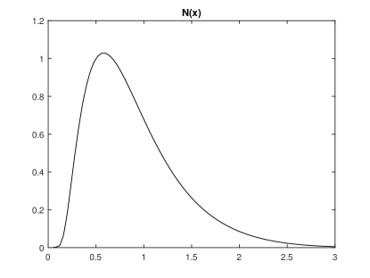
We use a regular grid on with points. For the evolution process, we use a regular grid on , with points. We plot the function in Figure 1.
6.3 Reconstruction of and .
We now consider a noisy approximation for the eigenpair , obtained by adding a random noise to the data. That is, we assume that
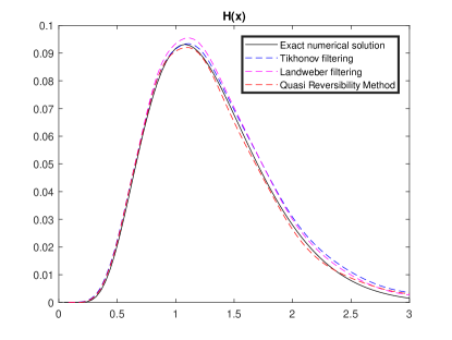
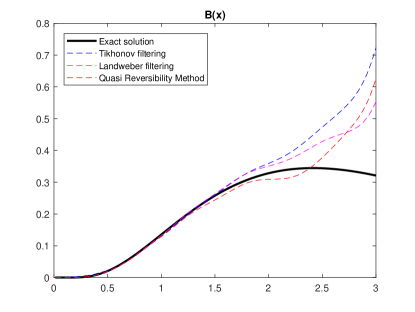
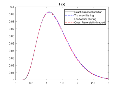
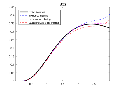
where are random noises uniformly distributed in . We recover the approximation using the noisy measurement . We plot the approximation for different noise levels . Here, we use the values (Figure 2), and (Figure 3). The parameters used are for the Tikhonov method and for the Landweber method.
To recover the fragmentation rate from we use the truncate division by . That is, we define if and zero otherwise. The following figures show the recovered function for the parameters , and . Observe that the instabilities near of the reconstructed function are due to the fact that the fast decay of near affects the truncated division.
6.4 Numerical Error.
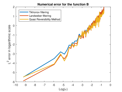
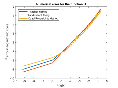
We compare the numerical error of the reconstructions of the functions and for small values of . Here, we use the norm to estimate this error. This norm is computed using rectangular integration. For this experiment, we assume that . We plot the error in logarithmic scale in Figure 4. Observe that for small values of the Landweber filter gives a better reconstruction, which is following our theoretical results.
7 Conclusion
In this article, we treated the inverse problem for the growth-fragmentation equation of a wide class of transition probabilities. Namely, we deal with transport probabilities which are generalizations of self-similar probabilities. We developed a new approach to regularize the inverse problem associated with the transport probabilities. Our approach is based on the Fourier transform theory for locally compact groups. We regularized the Fourier transform of differential operators using several filters in the spectral variable, such as modifications of the Landweber and Tikhonov filters.
For each method, we obtained their respective error estimates. The Landweber method provides an algorithm to recover the fragmentation rate , with order , where is the degree of smoothness of , as proved in Theorem 4.4. The error obtained using the Landweber method is better compared with other methods. This fact was verified by numerical simulations.
Our theoretical approach has been focused on transport operation induced by diffeomorphisms. A natural continuation of this work is to deal with transport operations induced by arbitrary functions. Another possible follow-up is to apply our methodology to problems arising in data science, as well as biological problems as in [20, 21].
One potential application of the problem under consideration concerns modeling normal prion protein (PrP(C)) and infectious prion protein (PrP(Sc)) populations interacting in an infected host [5]. Indeed, Perthame and Doumic in [22] proved key asymptotic results for the stable population where our results could be applied.
We note that even in the particular zero-growth case, , we have an interesting topic for further exploration since it allows for some simplifications in the operator of Equation (3). In such cases Doumic et al. [23] have addressed the issue of reconstructing the conditional probability kernel under a self-similar assumption and knowledge of the fragmentation rate . This shall be addressed in a future publication.
Acknowledgements
AAG and JPZ acknowledge support from the FSU-2020-09 grant from Khalifa University. The authors acknowledge the financial support provided by CAPES, Coordenação de Aperfeiçoamento de Pessoal de Nível Superior, grant number 88887.311757/2018-00, CNPq, Conselho Nacional de Desenvolvimento Científico e Tecnológico, grant numbers 308958/2019-5 and 307873/2013-7, and FAPERJ, Fundação Carlos Chagas Filho de Amparo à Pesquisa do Estado do Rio de Janeiro, grant numbers E-26/200.899/2021 and E-26/202.927/2017.
References
References
- [1] Benoit. Perthame. Transport Equations in Biology. Frontiers in Mathematics. Birkhäuser Basel, 2006.
- [2] Johan A. Metz and Odo. Diekmann. Formulating models for structured populations. In Johan A. Metz and Odo. Diekmann, editors, The Dynamics of Physiologically Structured Populations, pages 78–135, Berlin, Heidelberg, 1986. Springer Berlin Heidelberg.
- [3] Britta Basse, Bruce Baguley, Elaine Marshall, Wayne Joseph, Bruce van Brunt, Graeme Wake, and David Wall. A mathematical model for analysis of the cell cycle in cell lines derived from human tumors. Journal of mathematical biology, 47:295–312, 11 2003.
- [4] Philippe Laurençot and Benoit Perthame. Exponential decay for the growth-fragmentation/cell-division equations. Commun. Math. Sci., 7(2):503–510, 06 2009.
- [5] Meredith Greer, Laurent Pujo-Menjouet, and Glenn Webb . A mathematical analysis of the dynamics of prion proliferation. Journal of theoretical biology, 242:598–606, 11 2006.
- [6] François Baccelli, David McDonald, and Julien Reynier. A mean-field model for multiple tcp connections through a buffer implementing red. Performance Evaluation, 49:77–97, 09 2002.
- [7] Benoît Perthame and Lenya Ryzhik. Exponential decay for the fragmentation or cell-division equation. Journal of Differential Equations, 210(1):155–177, 2005.
- [8] Philippe Michel, Stéphane Mischler, and Benoît Perthame. General entropy equations for structured population models and scattering. Comptes Rendus Mathematique, 338(9):697–702, 2004.
- [9] Marie Doumic, Pedro Maia, and Jorge Zubelli. On the calibration of a size-structured population model from experimental data. Acta biotheoretica, 58:405–13, 12 2010.
- [10] Marie Doumic, Benoit Perthame, and Jorge Zubelli. Numerical solution of an inverse problem in size-structured population dynamics, in "inverse problems. Inverse Problems, 25:045008, 04 2009.
- [11] Thibault Bourgeron, Marie Doumic, and Miguel Escobedo. Estimating the division rate of the self-similar growth-fragmentation equation. Inverse Problems, 30, 01 2014.
- [12] Benoit Perthame and Jorge P Zubelli. On the inverse problem for a size-structured population model. Inverse Problems, 23(3):1037–1052, apr 2007.
- [13] Marie Doumic and Léon Tine. Estimating the division rate for the growth-fragmentation equation. Journal of mathematical biology, 67, 06 2012.
- [14] Walter. Rudin. Fourier Analysis on Groups. Wiley Classics Library. Wiley, 1990.
- [15] J.D. Zuazo. Fourier Analysis. American Mathematical Soc., 2001.
- [16] Heinz Engl, Martin Hanke, and Andreas Neubauer. Regularization of Inverse Problems. Mathematics and Its Applications. Springer Netherlands, 1996.
- [17] R. Lattès and J.-L Lions. Méthode de quasi-réversibilité et applications. Travaux et recherches mathématiques. Dunod, 1967.
- [18] T. Kato. Perturbation Theory for Linear Operators. Springer Berlin Heidelberg, 1995.
- [19] Marie Doumic and Pierre Gabriel. Eigenelements of a general aggregation-fragmentation model. Mathematical Models and Methods in Applied Sciences, 20:757–783, 07 2009.
- [20] Jean-Baptiste Bardet, Alejandra Christen, Arnaud Guillin, Florent Malrieu, and Pierre-André Zitt. Total variation estimates for the TCP process. Electronic Journal of Probability, 18, 2013.
- [21] Fadia Bekkal Brikci, Jean Clairambault, and Benoǐt Perthame. Analysis of a molecular structured population model with possible polynomial growth for the cell division cycle. Mathematical and Computer Modelling, 47(7):699–713, 2008.
- [22] Juan Calvo, Marie Doumic, and Benoît Perthame. Long-Time asymptotics for polymerization models. Communications in Mathematical Physics, 363(1):111–137, October 2018.
- [23] Marie Doumic, Miguel Escobedo, and Magali Tournus. Estimating the division rate and kernel in the fragmentation equation. Annales de l’Institut Henri Poincaré C, Analyse non linéaire, 35(7):1847–1884, 2018.