Accelerating Sparse DNNs Based on Tiled GEMM
Abstract
Network pruning can reduce the computation cost of deep neural network (DNN) models. However, sparse models often produce randomly-distributed weights to maintain accuracy, leading to irregular computations. Consequently, unstructured sparse models cannot achieve meaningful speedup on commodity hardware built for dense matrix computations. Accelerators are usually modified or designed with structured sparsity-optimized architectures for exploiting sparsity. For example, the Ampere architecture introduces a sparse tensor core, which adopts the 2:4 sparsity pattern.
We propose a pruning method that builds upon the insight that matrix multiplication generally breaks the large matrix into multiple smaller tiles for parallel execution. We present the “tile-wise” sparsity pattern, which maintains a structured sparsity pattern at the tile level for efficient execution but allows for irregular pruning at the global scale to maintain high accuracy. In addition, the tile-wise sparsity is implemented at the global memory level, and the 2:4 sparsity executes at the register level inside the sparse tensor core. We can combine these two patterns into a “tile-vector-wise” (TVW) sparsity pattern to explore more fine-grained sparsity and further accelerate the sparse DNN models. We evaluate the TVW on the GPU, achieving averages of , , and speedups over the dense model, block sparsity, and unstructured sparsity.
Index Terms:
Pruning, Sparse DNN, Sparse tensor coreI Introduction
Deep neural network (DNN) models have achieved and even surpassed human-level accuracy in important domains [1]. For instance, transformer-based models [2] in natural language processing (NLP) such as BERT [3] have dominated the accuracy in various NLP tasks. Despite their high accuracies, DNN models also have significant computational cost, both in training and inference. The inference latency of modern DNN models could also be excessively high due to the enormous computation cost and memory usage.
One particularly effective and promising approach to reduce the DNN latency is pruning [4], which exploits the inherent redundancy in the DNN models to transform the original, dense model to a sparse model by iteratively removing “unimportant” weight elements and retraining the model to recover its accuracy loss. In the end, the sparse model has fewer parameters and, theoretically, less computation cost.
The primary challenge in network pruning is how to balance the model accuracy and execution efficiency. Such a balance is fundamentally affected by the sparsity pattern that a pruning approach enforces. Intuitively, a stronger constraint on the sparsity pattern forces certain weights to be pruned and, thus, leads to lower accuracy, and vice-versa. The most fine-grained pruning approach leads to the so-called element-wise (EW) sparsity pattern, which prunes weight elements individually and independently, solely by their importance scores [4]. In other words, EW imposes no constraint on the sparsity pattern and can remove any weight element, leading to the minimal model accuracy degradation. However, the pruned sparse model also introduces irregular memory accesses that are unfriendly on commodity architectures. As a result, EW-based sparse DNN models usually run slower than the unpruned dense models on these architectures [5].
To realize the acceleration potential of sparse DNN models, researchers have proposed to co-design the sparsity pattern with hardware support. For instance, many architects have proposed various specialized accelerator designs [6] to exploit the zeros in the aforementioned EW pattern for latency reduction. Similarly, prior work proposes the vector-wise (VW) pattern [7] that divides a weight column to groups and prunes the same number of elements in a group. This sparsity pattern requires the new hardware or the modification of existing hardware [8]. Recently, NVIDIA has published GPU A100 with the Ampere architecture [9], which includes the sparse tensor core with the 2:4 (2-out-of-4) vector-wise sparsity. In summary, these approaches lead to sparse memory accesses and computation patterns that require hardware support.
In this work, we propose a novel algorithm that accelerate sparse DNN models on commodity DNN accelerators without hardware modification. Our key observation is that virtually all of today’s DNN accelerators implement dense general matrix multiplication (GEMM) [10] operations. GEMM-based accelerators [11, 12, 13, 14] are dominant owing to their wide applicability: convolution operations that dominate computer vision models are lowered to the GEMM operation, and NLP models are naturally equivalent to the GEMM operation. Examples include NVIDIA’s tensor core [11] and Google’s TPU [12] mentioned above. We propose a new pruning algorithm, which enforces a particular sparsity pattern on pruned models to directly leverage existing GEMM accelerators without modifying the microarchitectures.
In particular, our work exploits the key insight that the matrix multiplication on existing dense GEMM accelerators adopts the tiling approach, which breaks the large matrix into multiple smaller tiles for parallel execution. We propose a tiling-friendly sparsity pattern called tile-wise sparsity (or TW), which maintains a regular sparsity pattern at the tile level for efficient execution but allows for irregular, arbitrary pruning at a global scale through non-uniform tile sizes to maintain high model accuracies. To exploit the TW sparsity, we first divide the entire matrix into multiple tiles as in conventional tiled GEMM. We then prune the entire rows or columns of each tile according to the collective importance scores of each row and column. In our sparsity pattern, the tile size dictates the trade-off between model accuracy and execution efficiency. At one extreme where the tile size equals one, our TW sparsity is equivalent to the EW sparsity. At the other extreme where the tile size is the same as the matrix size, TW is equivalent to the global structural pruning that prunes rows or columns [5].
Building on top of TW, we further propose hybrid sparsity patterns. We can overlay the most fine-grained EW sparsity pattern on top of the TW sparsity and propose TEW sparsity. With a small fraction of EW (e.g., 1.5%), the TEW pattern significantly improves the accuracies of the TW-only sparse models. For the latest GPU architecture, TW is conducted at the global memory level, and the sparse tensor core of Ampere GPU [9] exploits 2:4 VW sparsity at the register level. Therefore, TW sparsity pattern is orthogonal to the VW sparsity pattern of the sparse tensor core. We can fuse the TW and VW and combine their advantages to build a more fine-grained pattern TVW and further accelerate the DNN models. We propose a pruning algorithm that iteratively shapes the weight matrix to meet our hybrid sparsity pattern constraint. Critically, our pruning algorithm dynamically allocates the sparsity budget to each layer to exploit the inherently uneven sparsity distribution across layers.
To maximize the algorithmic benefits of TW/TVW, we provide an efficient software implementation on commodity GPU hardware. Two key roadblocks arise as a result of the TW sparsity. First, TW naturally introduces frequently uncoalesced memory accesses due to the pruning pattern. Second, different tiles in TW could have different compute demands due to the different pruning degrees across tiles, which leads to load imbalance and GPU resource under-utilization. We address these challenges through a combination of intelligent data layout and concurrency/batching optimizations. TW and TVW achieve averages of and latency speedup on the tensor core with only negligible accuracy loss (1%-3%).
The contribution of our work is as follows:
-
•
Pattern Design.
We propose a tile-wise (TW) sparsity pattern to balance the model accuracy and execution efficiency on the existing dense accelerator. To further exploit the new sparse architecture, we propose the tile-vector-wise (TVW) sparsity which can fuse TW with the VW to achieve a more fine-grained sparsity pattern for the DNN pruning algorithm.
-
•
Pruning Algorithm.
We propose a multi-stage pruning algorithm that gradually shapes the weight matrix to TW pattern and dynamically allocates the sparsity budget at the layer level to overcome the uneven sparsity distribution.
-
•
Implementation.
We provide an efficient implementation of tile sparsity on commodity GPUs equipped with tensor core, and demonstrate significant speedups on state-of-the-art DNN models. We further optimize the implementation of TW with the compressed tile offset (CTO) to execute the TW in a single CUDA kernel.
-
•
New Hardware Support.
TVW sparsity can be implemented on the sparse tensor core of the newest Ampere GPU architecture [9] to achieve better accuracy at a high sparsity level and further accelerate DNN models.
II Background and Related Work
We summarize the recent efforts to reduce those models’ execution latency, which include building specialized hardware accelerators and applying algorithmic pruning optimization to reduce the size and computation cost of DNNs.
II-A Hardware Acceleration
We explain the computation characteristics of these models and common optimizations to reduce their execution latency.
Dense Model.
General matrix multiplication (GEMM) is a critical computation in the original dense DNN models. The fully connected layer and LSTM layer are native GEMM operations, while the convolutional layer can be converted to GEMM through the img2col transformation [15, 16]. The attention heads in BERT can also be computed with GEMM operations, and the computation of multiple heads could be combined into one large GEMM.
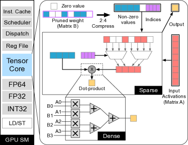
GEMM Acceleration. To reduce the model execution latency, NVIDIA adds tensor cores on the GPU since Volta architecture [11], which run a fixed size matrix multiplication. As shown in Fig. 1, the tensor core is essentially an accelerator for the GEMM. To exploit the DNN sparsity, NVIDIA upgrades the tensor core with a new 2:4 vector-wise sparsity feature that delivers a further doubling of throughput in the Ampere architecture [9], as shown in Fig. 1. The tensor core can also reduce the computation precision to FP16, Int8, and Int4 to support DNN quantization [17, 18, 19, 20, 21], which can also reduce the DNN model size. Our proposed sparsity is orthogonal to the quantization. Another example of the GEMM accelerator is TPU [12] which is based on a systolic array. The cuDNN [15] library implements different DNN layers for efficient execution on GPU, where the GEMM computation can use the closed-source cuBLAS library [22] or open-sourced CUTLASS library [23]. For large language models, some work [24, 25, 26] focused on optimizing the sparsity of self-attention operation with long sequences.

Sparse Model.
Recently, researchers have started to apply pruning [4] to DNN models, which exploit the inherent redundancy in the model to transform the original, dense model into a sparse model. In the end, the sparse model has fewer parameters and, theoretically, less computation cost. Executing sparse models relies on sparse matrix representation such as compressed sparse row (CSR) [22] and sparse GEMM operations, which are supported on GPU by cuSparse [22] library. However, as the GPU is initially designed for dense operations, the speedup of the sparse model over the dense model is usually negative unless the sparsity ratio is very large (over 95% reported by prior work [27]). As such, researchers begin to put various shape constraints on the pruning pattern and also propose to transform the existing architecture to execute those sparse models. For example, the recent work proposes new sparsity patterns that need to modify the existing dense GEMM accelerator [8, 6].
Unlike the prior microarchitecture-centric work, we propose a software-only acceleration of sparse DNN models on the dense GEMM accelerator, like the tensor core. We exploit the tile execution of GEMM computation and propose a tiling-friendly, tile-wise sparsity pattern to balance the model accuracy and compatibility for the dense GEMM accelerator.
II-B Sparsity Pattern
Many sparsity patterns [4, 8, 7, 9, 28] have been proposed to prune the weight tensors. Fig. 2 illustrates six sparsity patterns. For the sparse models, their weight tensors are static and pro-processed before the inference stage. However, for the activation tensors, the methods need to prune on the fly at runtime due to the irregular memory accesses. Therefore, these irregular patterns need unique software design, e.g., CSR representation for the element-wise pattern [22].
Element-wise.
Element-wise (EW) removes the individual weight element solely by its importance score rank. For instance, prior work [4] proposes to remove weight elements with small magnitude. This approach imposes no constraints on the sparsity pattern and could remove most of the weights among all pruning methods. Thus, it is also called unstructured pruning. However, the randomly distributed non-zero weights lead to substantial irregular memory accesses, which impose great challenges for efficient hardware execution. As such, researchers propose other two more structured pruning methods.
Vector-wise.
The second sparsity pattern shown in the middle of Fig. 2, vector-wise (VW) [8, 7], divides a column in the weight matrix to multiple vectors. Within each vector, it prunes a fixed portion of elements by the rank of their importance scores. This approach preserves the randomness within each vector for model accuracy. Meanwhile, it maintains the regular structure for efficient execution, where different vectors have the same number of non-zero weight elements. The GPU A100 [9] develops the sparse tensor core using the 2:4 VW sparsity pattern with fixed 50% sparsity.
Block-wise.
Block-wise (BW) [28] divides the weight matrix into small blocks, and treats a block as the basic pruning unit. In other words, the EW sparsity pattern is a special case of the BW sparsity pattern, which expands a block to an block. The structural sparsity pattern BW leads to the efficient execution of sparse models.
Tile-wise.
Tile-wise (TW) [29] pattern has two types, i.e., TW-C and TW-R, addressing vertical and horizontal dimensions of weight tensor and is based on the tiled GEMM algorithm, which is widely used in the GEMM accelerator [22, 23]. For each tile (sub-matrix), TW can simultaneously prune the column and row for the weight tensor. We will introduce the details in Sec. III.
Tile-vector-wise.
The last pattern is our proposed tile-vector-wise (TVW), which is a hybrid sparsity fusing TW and VW. We present the TVW design in Sec. III.
III Tile-wise and Hybrid Sparsity
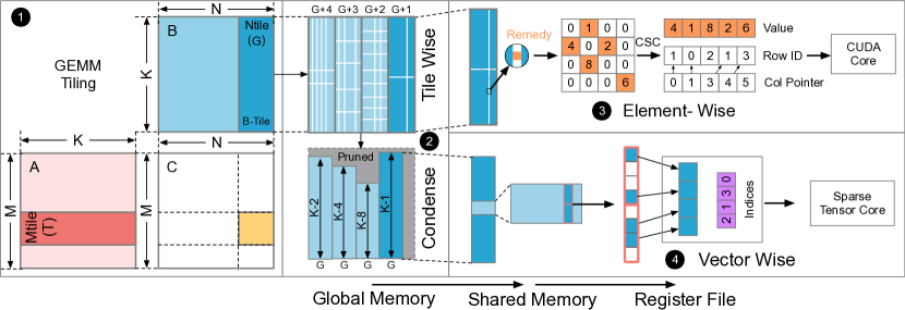
In this section, we present the details of our proposed TW, TEW, and TVW sparsity pattern. The TW sparsity pattern leverages the tiled execution of matrix multiplication, originally designed to exploit the parallel computation resources. The TW sparsity pattern introduces irregularity in the global matrix. Still, it maintains the computation regularity of individual matrix tiles exploiting the memory condensing approach crossing the shared and global memory. The VW sparsity pattern exploits the sparse tensor core to execute the 2:4 (2-out-of-4) VW sparsity at the register level. Therefore, these two patterns leverage different levels of GPU memory hierarchy, and TVW can be implemented simultaneously in a single CUDA kernel. We also show that the tile-wise sparsity pattern can be overlaid with the most fine-grained element-wise pattern (TEW) to increase the sparsity of pruned models and reduce their accuracy loss.
III-A Tiling and Pruning Co-design
As Sec. II explains, the dominant computation in deep neural network models is the general matrix multiplication (GEMM). In this subsection, we first present the details of tiled matrix multiplication. We then propose to co-design the matrix tiling and deep neural network pruning, which leads to the tile-wise (TW) sparsity pattern. We explain how TW maintains the compatibility on the dense GEMM accelerator and the composability with the fine-grained sparsity pattern.
Fig. 3 shows one level tiling of matrix multiplication on the GPU. The GEMM computes with input matrix (), weight matrix (), and output matrix (). Since modern high-performant microprocessors mainly adopt the manycore architecture, the tiled execution of output matrix breaks the entire GEMM computation into multiple ones such that they can run on multiple cores for parallel execution. Specifically, each core (or streaming multi-processor, SM in NVIDIA GPU) computes one tile with the size of (). Consequently, the core only loads rows of input matrix and columns of weight matrix (called ). With the output matrix tile size of , the weight matrix is divided to . The key idea of our TW pattern is to prune each with the regular column pruning (TW-C) and row pruning (TW-R) .
TW-C.
To improve the execution efficiency of the proposed sparsity pattern, we first perform the column pruning and for the weight matrix tile , which reduces its N-dimension size (i.e., width). Our approach prunes a different number of columns in each weight matrix tile for better irregularity. We use the example in Fig. 3 to illustrate its advantages. With the column pruning, the four tiles are pruned with 4, 3, 2, and 1 columns, respectively. Then, we re-organize the four tiles with , , , and columns. After pruning, the N-dimension sizes of the four tiles are .
TW-R.
The row pruning treats an entire row of each weight tile as the basic pruning unit, which leads to the reduced K-dimension size (i.e., height) of each . We prune each with the different number of rows determined by the pruning algorithm that we describe later. The difference across different tiles maintains the irregularity of sparsity required by model accuracy. E.g., the heights of four weight matrix tiles in Fig. 3 are , , , and respectively after the row pruning. The combined row and column pruning alleviates the constraint on the sparsity pattern and therefore allows more weight elements to be pruned.
TEW.
Since the TW still enforces a particular pruning pattern, important weight elements could be removed, leading to accuracy loss. We propose to overlay TW and EW to mitigate the accuracy loss. Fig. 3 illustrates the resulted hybrid pattern tile-element-wise (TEW). In order to prune percent of weights, the TEW first prunes percent of weights with only TW, and then restores percent of the weight elements with the highest importance scores. For the hybrid TEW pattern, each tile stores the EW pattern with the compressed sparse column (CSC) format. We leverage the linear property of matrix multiplication to execute the TW and EW separately. We explain the execution details in Sec. V.
TVW.
As shown in Fig. 3 , TW prunes the rows and columns at the global memory level. The newest Ampere GPU architecture adopts the sparse tensor core with the 2:4 VW sparsity pattern at the fine-grained register level to prune the two elements of each four-element vector, as illustrated in Fig. 3 .
Therefore, the VW sparsity is orthogonal with the TW sparsity, and we propose the hybrid TVW to fuse the VW and TW to complement each other. First, TW is a coarse-grained pattern. For example, TW-R prunes a row with elements, where is usually greater than . Fusing with VW can provide a more fine-grained pattern (2-out-of-4) to achieve a more irregular sparsity pattern. Second, due to the specificity of hardware design, the sparse tensor core has a fixed sparsity for every four-element vector. TW has a more uneven sparsity distribution, which can benefit the accuracy, as we explain in Sec. VI-C. Finally, TVW also has efficient execution supported by the sparse tensor core.
Owing to the existence of globally uneven sparsity distribution and the irregularity inside the vector, TVW leads to a pattern that is closer to EW than the VW pattern. TVW/TW also removes more weights than BW owing to its fewer constraints on the pruning shape.
IV Tile Sparsity Based Pruning
This section explains our multi-stage pruning algorithm for leveraging the proposed TW sparsity pattern. Algorithm 1 describes the algorithm, which we explain in detail as follows.
Overview.
We adopt the multi-stage pruning algorithm that gradually prunes the pre-trained dense model to reach a target sparsity. Each iteration from Line 4 to 6 in Algorithm 1 is a complete pruning-tuning stage. Each stage consists of a pruning and fine-tuning step, where the algorithm first prunes the model with a small sparsity target and then fine-tunes the pruned model to restore the model accuracy. Line 4 increments the sparsity target in the current stage with the sparsity step (). The “PrunePattern” in Line 5 corresponds to the functions in Algorithm 2 and 3, depending on the pruning strategy. Prior work points out that multi-stage pruning improves the model accuracy more than single-stage pruning [4].
Pattern Pruning.
Algorithm 2 shows the EW, VW, and BW sparsity pattern pruning algorithm. For all patterns, we first split the weight tensor according to their pruning granularity. For EW, we regard each element as the individual pruning granularity. And VW splits by the vector with shape of the and BW with the block. Then, we derive their importance score, which is introduced in next. We can easily sort them and get the pruning threshold by the percentile function with the target sparsity . Finally, we can prune the elements (or blocks) according to the threshold. Algorithm 3 presents the TW-based algorithms, including TEW and TVW. As explained in Sec. III, the TW pattern requires the column pruning before the row pruning. We first equally divide the sparsity for the TW-C and TW-R (Line 2). Then, we break the weight matrix into column-based tiles (Line 3) and evaluate the importance score of each tile (Line 4). We then determine the threshold for TW-C pruning based on the sparsity target caculated before (Line 5). Line 6-8 remove the column tiles. Afterward, we reorganize the column-pruned matrix into tiles (line 9). Line 10-16 performs TW-R pruning, which is similar to TW-C pruning. After the column and row pruning, the weight matrix becomes compatible with TW. In our algorithm, we design the tiling granularity as a tunable hyper-parameter, through which we explore the trade-off between the accuracy and performance of the sparse model. For the TEW sparsity pattern, we first add more sparsity for TW (Line 19) and execute the TW pruning (Line 21). Then we exploit the remedy algorithm (Line 23-28) to restore the EW sparsity. For the TVW sparsity pattern, we can combine and orderly execute TW (Line 32) and VW (Line33) pruning with precise sparsity division (Line 31).
Global Weight Pruning.
There exists an uneven distribution of weight sparsity in different layers of a DNN model, which previous work [29] uses a global weight pruning to exploit. Taking Algorithm 3 as an example, the codes in Line 5 and line 12 sort the scores for all tiles in the column and row pruning, respectively. The codes in Line 6-9 and Line 13-16 prune the tiles from all layers in the DNN model according to their importance rank.
Importance Score.
How to compute the importance score is an active research topic [4, 30, 31]. The most intuitive approach [4] is to use the weight’s absolute value. We use a more accurate approach [31] that uses the incurred error by removing a parameter as its importance score.
V Efficient GPU Implementation
This section introduces our efficient GPU implementation that unleashes the algorithmic benefits of TW. Exploiting the unique sparsity pattern of TW, we first describe the basic tiling design, followed by three key optimizations that combine intelligent data layout and concurrency/batching optimizations to maximize the efficiency of TW tiling on tensor cores.
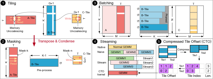
The advantage of TW sparsity pattern is that sparse matrix multiplication could be transformed to dense GEMM, which can be effectively accelerated on dense GEMM accelerators such as the tensor core on GPUs (Sec. III). Fig. 4 shows how we transform sparse matrix multiplication that has the TW sparsity pattern to a dense GEMM, and how it exploits various GPU characteristics to maximize the performance.
Tiling.
We start by tiling matrices as usual. Fig. 4 illustrates an example, where generating an output tile requires two input tiles and . Each input matrix tile has two mask vectors that indicate which rows and columns in the matrix tile are pruned. In the example of , the white rows and columns are pruned. We remove the pruned rows and columns in the weight matrix tile , which can be done offline before the model inference starts. The input tile and output tile are stored in the original dense format. Their pruned rows/columns are skipped rather than removed.
We modify the dense GEMM kernel such that it skips computing partial sums for pruned elements according to the mask vectors. This reduction of computation is the source of acceleration. Our baseline GEMM implementation is based on the open-sourced CUTLASS [23], which is a high-performance linear algebra CUDA library. It implements three levels of tiling to maximize the data reuse in the global memory (thread block tile), shared memory (warp tile), and register file (thread fragment). Meanwhile, it can also leverage the tensor core in the GEMM computation, which we use to accelerate the TW.
However, a naive tiling implementation is inefficient and even causes slowdown compared to the original dense model. In our implementation, we exploit three optimizations that mitigate the inefficiencies and maximize the benefits of TW.
Memory Accesses Coalesce.
Naive tiling leads to frequent uncoalesced memory accesses that are inefficient on the single-instruction-multiple-data based GPUs. Fig. 4 shows the memory access patterns in the original row-major matrix format. The pruned row in causes the skip of column in . Therefore, a continuous access to the (marked by the yellow arrows) that is originally coalesced now becomes uncoalesced, which can cause severe performance degradation as uncoalesced memory accesses require multiple memory transactions. The uncoalesced accesses also exist in the matrix tile (marked by the red arrows) owing to the pruned column in .
We propose to store the matrix tiles in their transposed format to optimize their memory access efficiency. In Fig. 4 where the three tiles are transposed, the column skipping is converted to the row skipping. Thus, it eliminates the uncoalesced accesses and improves the access efficiency.
Load Imbalance Mitigation.
TW sparsity inherently introduces imbalanced tiles. That is, some tiles will require more computations since fewer rows are pruned; other tiles that have more rows pruned will lead to lower computation. Imbalanced tiles lead to resource under-utilization, and thus affects the overall speedup. We propose to batch tile computations to improve the utilization. Fig. 4 shows an example where the weight matrix is decomposed into tiles, where is the TW granularity. Different are batched together to share the same . Batching improves resource utilization as a batched GEMM packs multiple tiles and thus increases the computation.
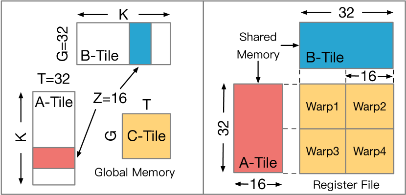
Another practical benefit of batched-GEMM implementation is that we can reuse existing high-performance tensor core-based GEMM kernels and avoid implementing specialized GEMM kernels, each customized for a particular tile size. Fig. 5 illustrates the warp-level tiling and Listing 1 shows the kernel implementation that uses tensor core APIs. We assume that , and , which is the minimum tiling granularity as it must be the multiple of (i.e., warp size). and are stored into the shared memory and to the register file. Then a warp tile will compute the out-product with the tensor core MMA API, which can support the fixed size () matrix multiplication.
While batching mitigates resource under-utilization, we find that it is possible that the computation of a batch still under-utilizes the GPU resources. Our previous work [29] leverages concurrent kernel execution on modern GPUs [32] to further improve resource utilization. In the studied NVIDIA GPU platform, we overlap the computation of different tiles by assigning to different streams, and rely on the underlying scheduler to maximize resource utilization. Fig. 4 shows an example where naively running different batches could have lower performance than the original unpruned GEMM. Concurrently executing multiple batches with different streams improves performance.
Tile Fusion and Compressed Tile Offset.
The stream GEMM in Fig. 4 launches multiple kernels, each with two mask vectors. And all kernels execute concurrently within different streams. The resource utilization can be further improved by fusing the computation of all tiles into only one kernel. Inspired by the compressed sparse column (CSC) method, as shown in Fig. 4 , we change the tile mask into the index of the unpruned row/column. As such, the tile index will have more memory efficiency compared to the tile mask when the sparsity increases.
First, we fuse all tile computations with a two-dimension tile index with tile length number, as shown in Fig. 4 . For example, the two tiles have three rows (1, 2, 4) and two rows (0, 3) to compute, respectively. Instead of using multiple tile masks to indicate which columns are pruned for each tile, we merge and pad them into a matrix and launch one kernel for the GEMM. This method takes full advantage of the concurrency and allows schedulers to maximize resource utilization at the thread block level.
Second, we continue to change the indices of row/column to the offsets, which are friendly to the GPU global memory access. For example, the GPU needs to access the first tile with original indices (0, 1, 2). We only add the offsets (1, 1, 2) with the original indices and change them to (1, 2, 4). Then the GPU can efficiently and correctly find the memory address. The tile offsets are friendly to the global memory access mechanism and improve memory access efficiency.
VI Evaluation
In this section, we demonstrate that TW is able to maintain the accuracy of sparse DNN models and provide the significant execution speedup over the dense model and other sparsity patterns at the same time. We first explain our evaluation methodology with the use of state-of-the-art DNN models on the GPU equipped with (sparse) tensor cores. We then study the design space of TW to explore the trade-off between model accuracy and latency. In the end, we select the representative configurations of TW and TVW and compare it with other sparsity patterns.
VI-A Methodology
Benchmark.
We evaluate five popular neural networks, VGG16, ResNet-18, ResNet-50 (CNN), NMT (LSTM), and BERT (Transformer), which cover tasks from the computer vision and NLP domain.VGG16 [33], ResNet-18 [34], and ResNet-50 [34] are popular CNN models. We evaluate its accuracy for image classification on the ImageNet [35] dataset with 1.2 million training images and 50,000 validation images. We prune its weight matrix after applying the img2col method [15], which flattens the filters in the same channel to a column and different columns correspond to different channels (so the left flattened feature map matrix multiplies the flattened weight matrix in Fig. 3). This approach is similar to prior work [8].
We evaluate the accuracy of NMT model, which adopts the attention based encoder-decoder architecture, for the machine translation task. We reproduce the model with an open-source framework [36]. We evaluate the NMT model on the IWSLT English-Vietnamese dataset [37], and use the BLEU (bilingual evaluation understudy) score [38] as the accuracy metric. For the Transformer model family, we use the BERT-base with layers. The two evaluated downstream tasks are the sentence-level classification on the widely used GLUE (general language understanding evaluation) dataset [39] and the more challenging question answering task on the SQuAD dataset [40]. The GLUE dataset is a composite dataset with 10 different sub-tasks, and we evaluate 6 out of them.
In our experiments, we use the pre-trained models that can achieve their reported reference accuracies. We then apply EW, VW, BW, and our proposed TW, TEW, and TVW sparsity patterns to prune the dense models according to the algorithm described in Sec. IV. To conduct a fair comparison, we strictly set the same hyper-parameters (such as learning rate) for all patterns and fine-tune with the same epochs for each sparsity step. We use the PyTorch [41] and TensorFlow [42] framework for fine-tuning. Depending on the dataset size, we perform the fine-tuning for 4-10 epochs at each target sparsity level for BERT and NMT, which is sufficient to saturate the model accuracy in our experiment. For CNNs, we follow the pruning work [43] to fine-tune the pruned models with 100 epochs.
Baselines.
We compare the proposed TW, TEW, and TVW with EW, VW, and BW. For accuracy, we evaluate all patterns on the DNN models after fine-tuning. Especially for the VW, there are two different settings. First, the sparse tensor core of the latest NVIDIA Ampere GPU architecture [9] adopts the 2:4 (2-out-of-4) pattern with fixed 50% sparsity. Second, the previous research [8] proposed another type of sparse tensor core [8], which has the 4:16 (4-out-of-16) pattern with a fixed 75% sparsity. As such, we conduct two settings for VW, VW-4 for the real GPU A100 with 2:4 sparsity and VW-16 for n:16 sparsity, which we only use for accuracy comparison because it can not be accelerated supported by the existing GPUs.
For the latency evaluation, we execute EW and BW using the latest cuSparse [22] library. We also implement BW with the BlockSparse library in the Triton [44]. Surprisingly, the two kinds of block sparsity implementation (i.e., Triton and cuSparse) perform similarly because they use the same algorithm and programming model based on CUTLASS [23]. Finally, we choose the cuSparse as our baseline in this paper.
Our TW-based implementation (Sec. V) is based on CUTLASS [23], an open-source, high-performance GEMM template library. For the VW-4, we evaluate it on the GPU A100 with CUTLASS sparse implementation for the sparse tensor core. For TVW, we combine and implement the TW patterns on the VW-based sparse version of CUTLASS. For all those libraries, including TW, we modify the original model codes to call each library explicitly. In this paper, we focus on the GEMM execution time.
We conducted on the Tesla A100 GPU [9], which is added with the sparse tensor core. Therefore, we only evaluate the VW-4 benchmark on A100. The EW runs only on the CUDA core with the cuSparse library and the BW implementation can run on the tensor core supported by cuSparse library. The convolution operations in the CNN workloads are converted to GEMM by the img2col method [15]. The models are all trained using FP32. All inferences on the CUDA core are done using FP32, and all inferences on the tensor core are done using FP16.
We label all pruning patterns by XX-YY, where XX represents the pruning pattern, and YY is the granularity. For example, TW-64 means TW adopts granularity . In particular, VW-4 and VW-16 represent VW with the 2:4 pattern and n:16 pattern, respectively.
VI-B Design Space Exploration
We now study the design space of TW, which is the tiling granularity , to explore the trade-off between model accuracy and latency. In addition, we also evaluate the hybrid TEW pattern, which extends the trade-off space in sparse models.
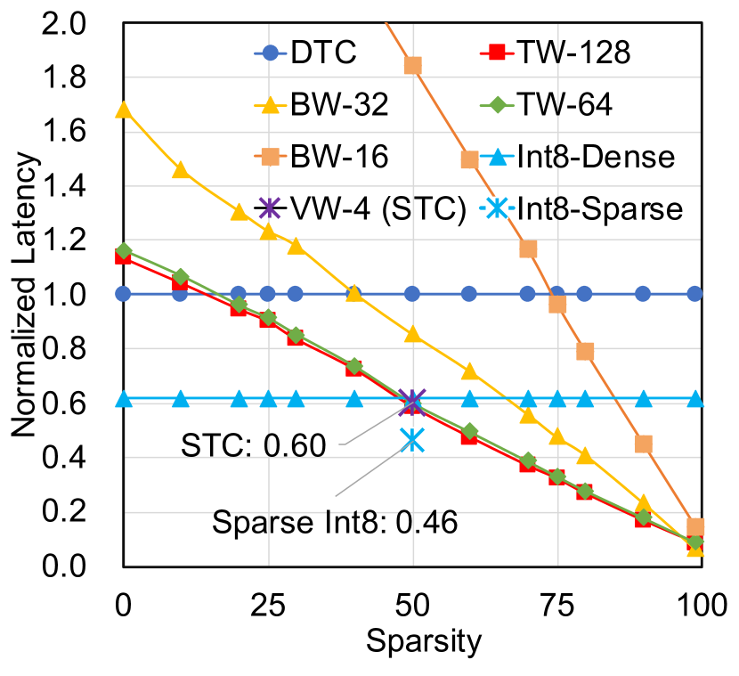
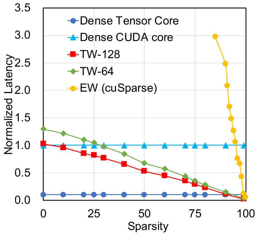
We first explore the impact of tiling granularity for TW and BW pruning. As shown in Fig. 6(a) and Fig. 6(b), we compare the normalized latency of EW, VW, BW, and TW. VW and BW can only be supported by the (sparse) tensor core of A100. EW can only run on the CUDA core implemented by cuSparse. Our proposed TW and TVW pattern can run on both tensor cores and CUDA cores. All experiments are conducted on the GEMM with shape ().
Speedup.
The tiled GEMM performance greatly corresponds to the tiling size (granularity). Smaller tiling size leads to less computation in the thread-block (SM) level tile but more global memory accesses, leading to a lower utilization ratio of SM and degraded performance of GEMM, and vice versa. TW-128 and TW-64 have similar latency-sparsity trends because we optimize the tiling size settings. As illustrated in Fig. 5, we can adjust the of corresponding to the granularity of . and are independent due to the design of TW. in TW-64 is twice as big as that in TW-128, then they have the same computation operations and global memory usage for each thread-block (SM) level tile. TW-128 can surpass the performance of dense GEMM when the sparsity threshold is just larger than 10% and 5% on the tensor core and CUDA core, respectively. In contrast, the sparsity threshold of BW-32 and BW-16 are 40% and 70% on the tensor core due to their smaller tiling size ( or ). VW-4 is exactly the GEMM on the sparse tensor core and achieves the fixed speedup compared to the dense GEMM on the tensor core. EW needs more than 95% sparsity to be better than the dense GEMM on the CUDA core. We also combine the dense tensor core results normalized to the dense CUDA core in the Fig. 6(b). There is a significant advantage (about speedup) of the tensor core over the CUDA core because GPU A100 [9] provides compute capability (TOPs, tera operations per second) over the CUDA core (19.5 TOPs FP32) for the tensor core (312 TOPs FP16). In summary, with the optimizations in Sec. V, the TW achieves the best performance on the tensor core and CUDA core among all sparsity patterns.
Int8 Quantization.
We also compare the performance against the quantization method: Int8 quantization (dense) and Int8 quantization with VW sparsity (sparse), i.e., sparse tensor core with Int8 quantization. The Int8-Dense achieves speedup over the dense GEMM and is similar to VW-4 because they have exactly equivalent memory footprint and computation load, which are 50% of original FP16 models. The Int8 with VW-4 sparsity can achieve a further speedup with 25% memory and computation of FP16 models.
Accuracy.
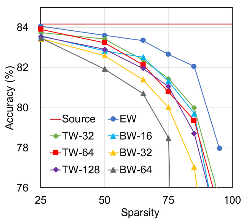
Fig. 6(c) compares the accuracy of EW, BW, and TW. The analysis is case-studied on the BERT model for sentence pair entailment task on the MNLI dataset. The most fine-grained EW achieves the best model accuracy as expected. When sparsity is less than , all the granularities evaluated have similar accuracies except BW-64, suggesting that the BERT model is at least 50% redundant. In particular, at a sparsity of 75%, our proposed TW-128 has an accuracy loss of about 1.6% compared to EW. As the sparsity increases, the accuracy drop becomes more significant. The most coarse-grained BW-64 experiences the most drastic accuracy drop of at 75% sparsity. The accuracy of BW-64 is unacceptable for the DNN model, and BW-32 also has a gap compared to TW. The accuracy drop of TW increases slightly with a larger value. This is because the larger value puts a more strict constraint on the pruning shape, but larger also means greater latency reduction. We find that of 128 and 64 are sufficient to maintain the model accuracy while providing significant latency reduction.
This comparison shows that TW has a significant advantage over other sparsity patterns. To reduce the experiment exploration space, we first make TW and BW have similar accuracy trends and then compare their latency. Therefore, we set BW with for the following experiments and set TW/TVW with for CNN models and for NMT and BERT models in the rest experiments of this section.
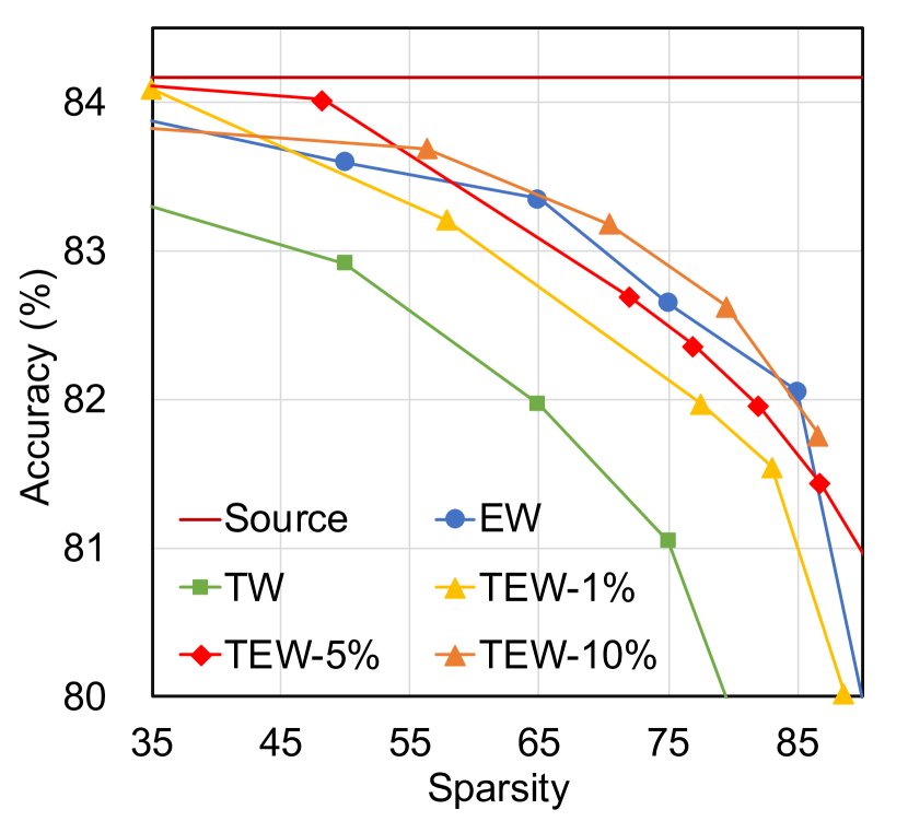
Impact of in TEW.
We evaluate the impact of in TEW, which determines the amount of EW pattern imposed on TW (Sec. III). Fig. 7(a) compares the sparse BERT model accuracy of different sparsity levels with EW, TW, and TEW patterns. The accuracy of the sparse model with TW is lower than EW. On the other side, TEW can mitigate the accuracy loss in TW by adding a small portion EW, which is controlled by the parameter in Sec. III-A. For instance, with , the TEW accuracy catches up with EW, and TEW-10% surpasses EW.
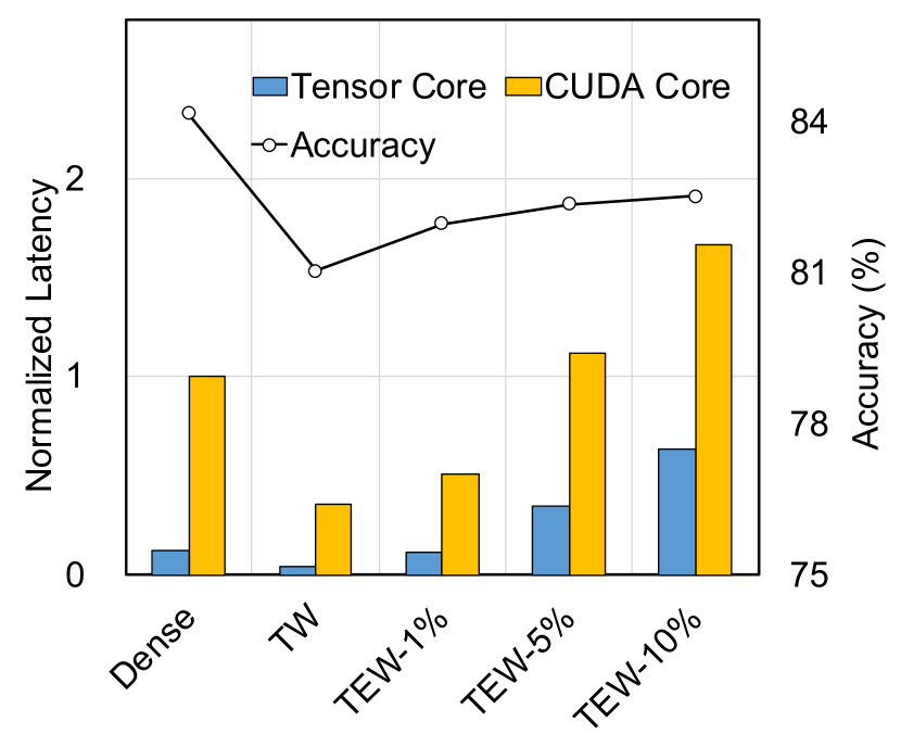
Fig. 7(b) compares the latency (left -axis) and accuracy (right -axis) of the dense model and various TW and TEW models with the fixed 75% sparsity. We show the latency results on both tensor core and the CUDA core, which are all normalized to the dense model latency on CUDA core. On the tensor core, TW achieves speedup than the dense model. TEW achieves no speedup at compared to the dense model, and its performance is worse as increases. This is because the irregular portion of TEW (i.e., the EW portion) could not be executed on the dense tensor cores and, instead, has to be executed on the CUDA cores, which is about 8 slower than the tensor cores. To illustrate the point, we show the results of running different sparse models on CUDA cores only. Using CUDA cores alone, TEW with is about faster than the dense model. Thus, we expect that TEW is useful in resource-constraint scenarios such as mobile systems.
VI-C Accuracy Comparison
We compare the accuracy and latency speedup of TW with EW, VW, BW on three different models. We perform the comprehensive evaluation of BERT model for the sentence classification task on the composite GLUE dataset, which includes ten different datasets. We observe similar results on 6 studied datasets and therefore only report the result on the largest dataset MNLI. We also report its result on the question answering task with the SQuAD dataset. For the latency speedup, we report the results on the A100 GPU using tensor core and CUDA core separately.
Accuracy.
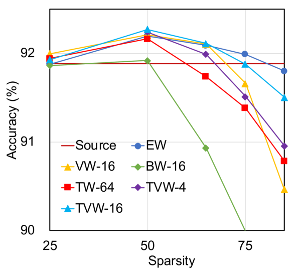
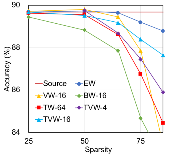
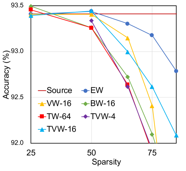
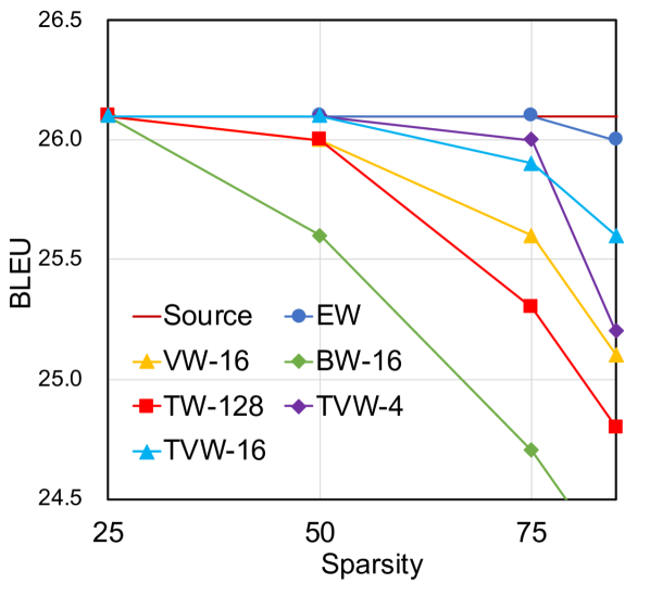
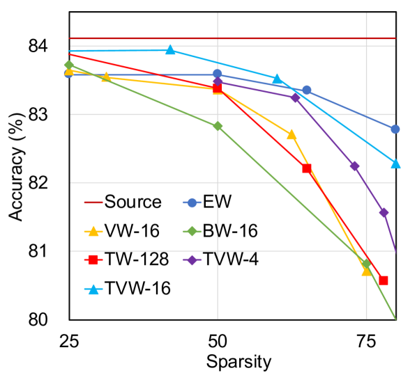
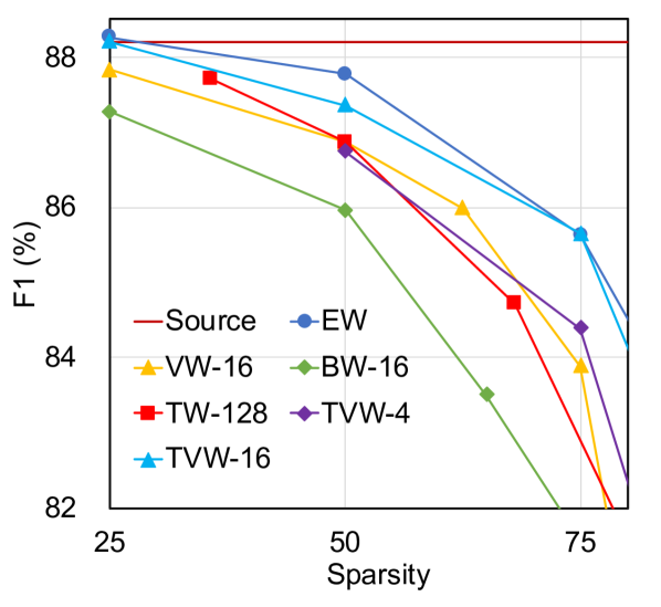
Fig. 8 shows the accuracy of different models with different pruning patterns. The granularity of TW and TVW is 64 (128) for CNN (NMT and BERT) and the block size of BW is , which balances the accuracy and latency speedup as our previous design space analysis suggests. We adopt top-5 accuracy for VGG, ResNet-18, and ResNet-50. The vector size of VW-16 is set to 16 as used in the original paper [8]. VW-4 is the original sparse tensor core 2:4 sparsity on A100. Therefore, we also have the TVW-4 and TVW-16 corresponding to the VW-4 and VW-16.
EW reaches the best accuracy of all the evaluated algorithms, and BW has the worst accuracy under the same sparsity except for the Resnet-50 model. BW has the largest granularity, which contains elements for each pruning. For ResNet-50, we checked the original pruning data and found that BW left some smaller layers (e.g., the first layer) without pruning, surprisingly improving accuracy. This indicates that TW can also get better accuracy if TW can also skip the smaller layers or apply more comprehensive metrics and algorithms.
VW-16 slightly outperforms TW when the sparsity is below 75%, owing to its irregularity inside the vector with a length of 16. With high sparsity (), TW generally outperforms the VW with the exception of NMT because TW has more flexibility for the high sparsity pruning and allows the uneven distribution of sparsity in a weight matrix. VW, BW, and TW experience a rapid accuracy drop compared to EW when the sparsity is over 75%, which suggests these models prefers irregular and unstructured sparsities.
Sparsity Pattern.
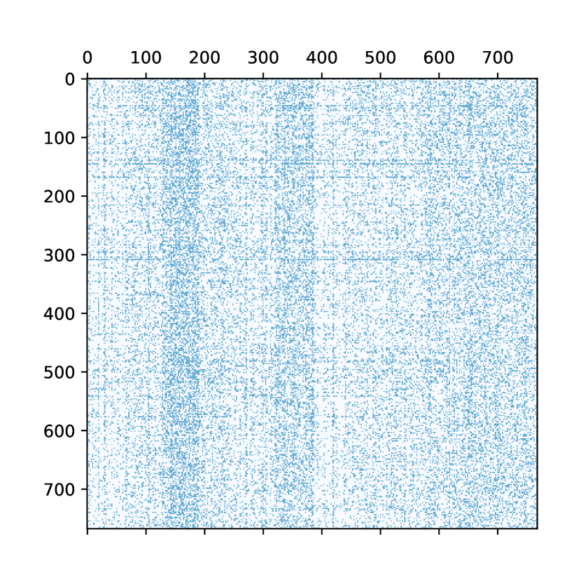
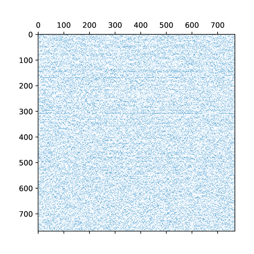
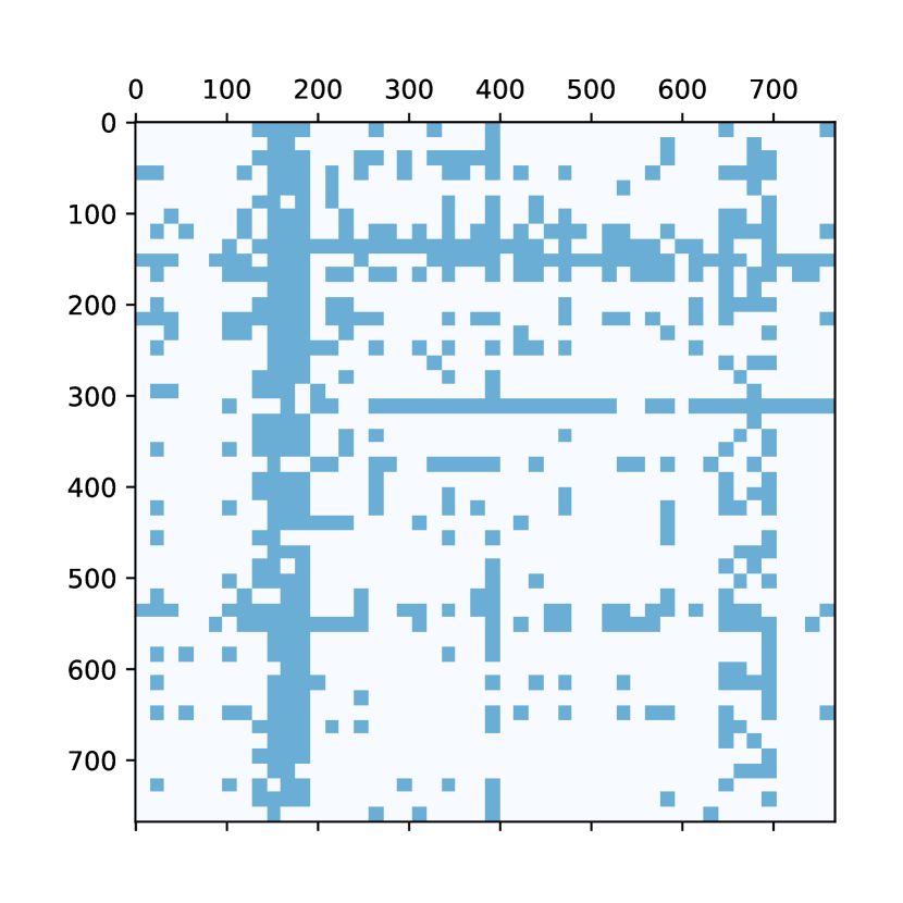
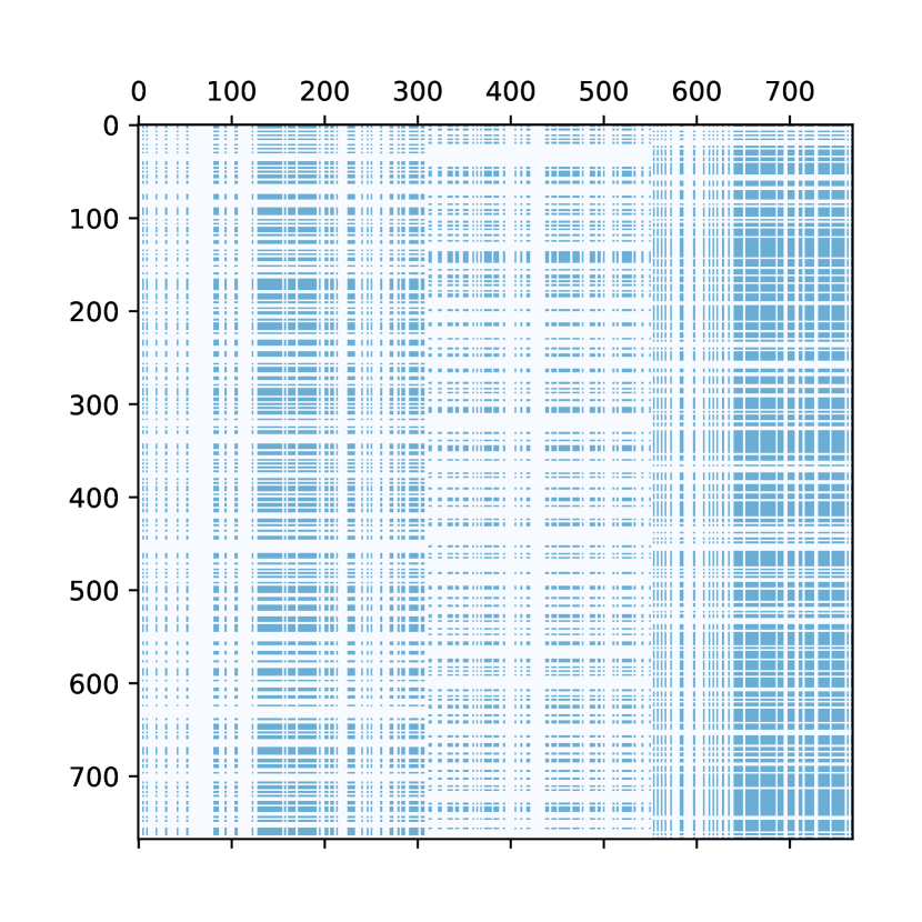
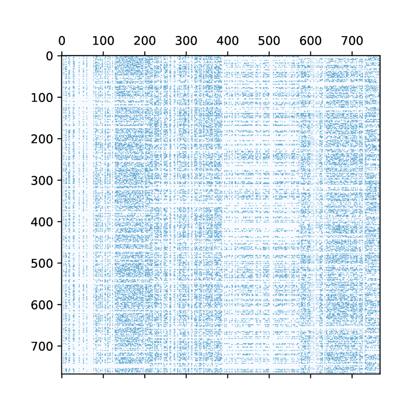
Fig. 9 shows the results of weight sparsity distributions of first layer of BERT under the sparsity for different patterns. The EW result shows that there exists uneven distribution across the matrix. And VW cannot fit this characteristic because it forces all prune units (vector) to have the same sparsity. Both BW and TW can adapt to this sparsity locality. However, the granularity of BW is too large and prunes complete square blocks, leading to too many blank areas and lower irregularity. In contrast, TW only prunes columns and rows inside a tiled block, maintaining higher irregularity, as shown in Fig. 9(d).
TVW contains the TW pattern and VW pattern. Therefore, TVW-4 in Fig. 9(e) is the most similar to the EW with high irregularity. TW prunes the weight tensor with the uneven distribution, and VW is irregular inside each vector. Naturally, TVW-16 can combine the irregularity of VW-16 and uneven distribution of TW and achieve significantly superior accuracy over the TW and VW-16. TVW-4 also benefits from the advantages of TW and VW-4 and surpasses the accuracy of TW. Still, the accuracy curve of TVW-4 is slightly lower than the TVW-16 because its vector size is smaller than TVW-16, and its pruning pattern is a fixed 2:4 (50%) sparsity pattern. As such, the curve of TVW-4 can only start from 50%, which is exactly the VW-4 sparsity without TW pruning. Fortunately, TVW-4 is supported by the existing GPU, but TVW-16 is not.
In summary, TVW combines the advantages of TW and VW, and achieves the second-best accuracy after the EW. This advantage of TVW can provide more potential opportunities to accelerate sparse models.
VI-D Speedup vs. Accuracy Comparison
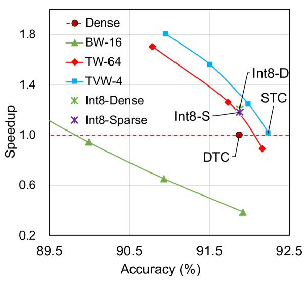
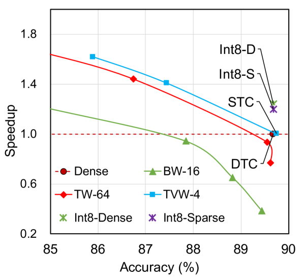
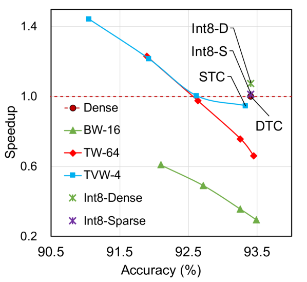
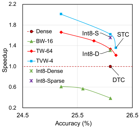
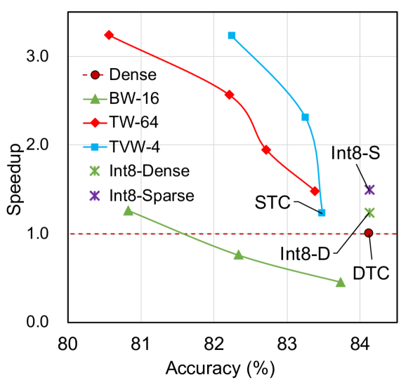
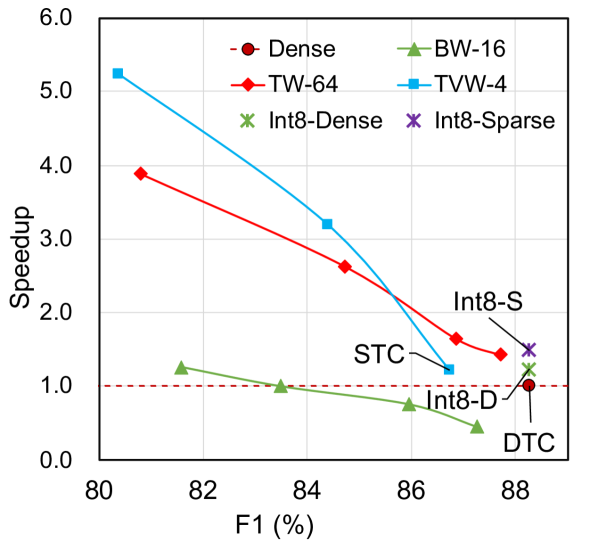
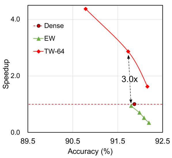
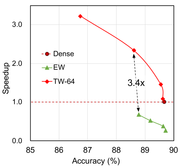
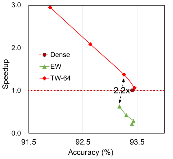
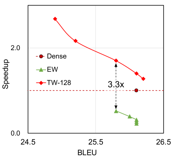
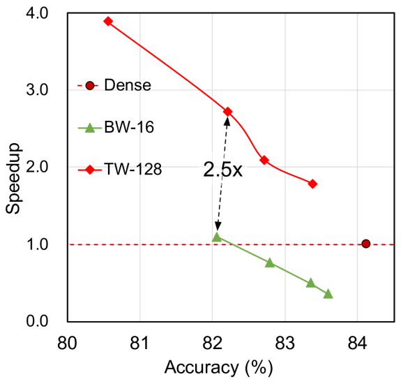
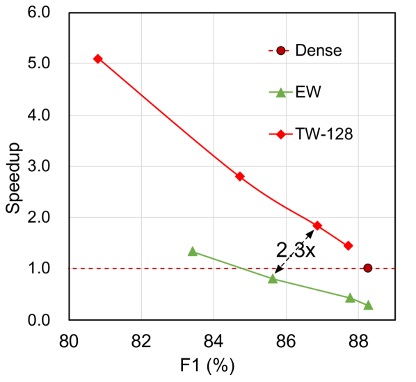
Fig. 10 and Fig. 11 compare the trade-off of latency speedup and model accuracy based on TW and other patterns including BW, VW on A100 (sparse) tensor core and EW on the CUDA core. We compare the TVW, TW, VW, and BW running on the (sparse) tensor core, and compare the TW and EW on the CUDA core. The granularity of TW and TVW is 64 for CNNs and 128 for BERT and NMT, the granularity of BW is 16, and TVW-4 employs VW-4, which is exactly the original sparse tensor core 2:4 pattern. As such, the starting point (STC) of the TVW-4 curve is the VW-4 results. EW can only run on CUDA core with cuSparse. The speedup is calculated against dense models on the tensor core and CUDA core separately. The experimental results demonstrate that TVW and TW can extend the latency-accuracy Pareto frontier on tensor cores. In contrast, other sparsity patterns lead to both longer latency and lower accuracy than the dense model. Finally, we compare the latency speedup of various patterns with the same level of accuracy drop (BERT with accuracy or F1 drop, VGG, ResNet-18, and ResNet-50 with top-5 accuracy drop, and NMT with BLEU drop).
Tensor Core.
For the tensor core results in Fig. 10, TVW achieves an average speedup of , and TW gets a speedup over the original dense GEMM. TVW performs best in most scenarios except for BERT on the SQuAD dataset and ResNet-50. We find that the SQuAD dataset is sensitive to sparsity. However, the minimum sparsity of TVW is the fixed 50% because of the hardware constraint from the sparse tensor core. Fortunately, TW complements this flaw of TVW at lower sparsity still with considerable speedup. For ResNet-50, TW and TVW have almost the same trends after 50% sparsity because they also have similar accuracy trends in Fig. 8(c).
From the perspective of VW-4 (i.e., the STC point), VW-4 achieves an average of speedup for the NMT and BERT on MNLI and SQuAD, but there is no () speedup for CNN models (VGG, ResNet-18, and ResNet-50), whose shape of GEMM computation is smaller than Transformer-based (BERT) and NMT models. In addition, compared with the experiment of the large GEMM in Fig. 6(a), VW-4 gets speedup on the shape of (). Evidently, VW is significantly affected by the shape of GEMM computation. In some corner cases, VW performs badly due to the inefficient execution of GEMM with a small shape. Combined with TW, TVW can be extended to a higher and more flexibale sparsity over VW-only pattern and achieve meaningful speedup for DNN models. Even though BW achieves better accuracy in some models (e.g., ResNet-50 in Fig. 8(c)), TVW still surpasses BW by because TVW adopts larger tiling size () but smaller granularity () for the tiled GEMM algorithm with high efficiency to run on GPU tensor core.
Int8 Quantization.
We also compare the Int8 quantization on the (sparse) tensor core. Based on our survey [45], the Int8 quantization exhibits almost no accuracy loss across all models. As for Int8-Sparse, we consider them as a reference in Fig. 10, given the absence of accuracy reports. We find that the Int8-Sparse has the same trends as the VW-4 (FP16) sparse pattern because they have a similar implementation on A100 GPU with the CUTLASS library. Due to the same reason, Int8-Sparse performs worse than Int8-Dense on CNN models, which have smaller GEMM shapes that are not friendly to the VW sparsity. For the Transformer-based models, Int8 can achieve meaningful speedups over FP16 dense models. Int8-Dense achieves , and Int8-Sparse has speedups. The speedup is fixed and marginal compared to the pruning-based TW and TVW, which can have higher performance and more flexibility.
CUDA Core.
For the CUDA core results in Fig. 11, TW achieves an average speedup of over the dense GEMM with the minor accuracy loss. In most models, EW cannot deliver meaningful speedups because EW is an unstructured pattern, leading large amount of irregular memory accesses. As such, TW is faster than EW with similar accuracy loss. Please notice that EW can only run on the CUDA core. Tensor core-based implementation performs a significant advantage (about speedup presented in Fig. 6(b)) over CUDA core. Therefore, when the accuracy of TVW is similar to the accuracy of EW, TVW outperforms speedup over EW.
In summary, TVW and TW achieve meaningful latency reduction on GPU due to their compatibility with dense GEMM, while all other sparsity patterns cause the slowdown. The design of TVW with more flexible sparsity can complement other sparsity patterns. That makes TVW can accommodate some resource-constraint scenarios, such as mobile systems.
VII Conclusion
In this work, we propose co-designing the tiling of matrix multiplication and DNN model pruning pattern to balance the irregularity for the model accuracy and compatibility for dense GEMM computation. We study an efficient software-only implementation of our proposed sparsity pattern, TW, that leverages the GPU’s tensor core accelerator and concurrency features. We further exploit the characteristic of the latest GPU A100 and design a more flexible sparsity pattern TVW combining the advantages from VW and TW. We demonstrate its capability of model accuracy preserving and high performance speedup on the state-of-the-art DNN models. Finally, TVW achieves significant and speedups over block sparsity and unstructured sparsity.
Acknowledgments
This work was supported by the National Key R&D Program of China under Grant 2021ZD0110104, the National Natural Science Foundation of China (NSFC) grant (62222210, U21B2017, and 62072297). The authors would like to thank the anonymous reviewers for their constructive feedback for improving the work. Any opinions, findings, and conclusions in this paper are those of the authors only and do not necessarily reflect the views of our sponsors.
References
- [1] U. A. ROMAN STEINBERG, “6 areas where artificial neural networks outperform humans,” https://venturebeat.com/2017/12/08/6-areas-where-artificial-neural-networks-outperform-humans/, 2018.
- [2] A. Vaswani, N. Shazeer, N. Parmar, J. Uszkoreit, L. Jones, A. N. Gomez, Ł. Kaiser, and I. Polosukhin, “Attention is all you need,” Advances in neural information processing systems, vol. 30, 2017.
- [3] J. Devlin, M.-W. Chang, K. Lee, and K. Toutanova, “Bert: Pre-training of deep bidirectional transformers for language understanding,” arXiv preprint arXiv:1810.04805, 2018.
- [4] S. Han, J. Pool, J. Tran, and W. Dally, “Learning both weights and connections for efficient neural network,” in Advances in neural information processing systems, 2015, pp. 1135–1143.
- [5] P. Hill, A. Jain, M. Hill, B. Zamirai, C.-H. Hsu, M. A. Laurenzano, S. Mahlke, L. Tang, and J. Mars, “Deftnn: Addressing bottlenecks for dnn execution on gpus via synapse vector elimination and near-compute data fission,” in Proceedings of the 50th Annual IEEE/ACM International Symposium on Microarchitecture. ACM, 2017, pp. 786–799.
- [6] Y. Wang, C. Zhang, Z. Xie, C. Guo, Y. Liu, and J. Leng, “Dual-side sparse tensor core,” in 2021 ACM/IEEE 48th Annual International Symposium on Computer Architecture (ISCA). IEEE, 2021.
- [7] Z. Yao, S. Cao, W. Xiao, C. Zhang, and L. Nie, “Balanced sparsity for efficient dnn inference on gpu,” in Proceedings of the AAAI Conference on Artificial Intelligence, vol. 33, 2019, pp. 5676–5683.
- [8] M. Zhu, T. Zhang, Z. Gu, and Y. Xie, “Sparse tensor core: Algorithm and hardware co-design for vector-wise sparse neural networks on modern gpus,” in Proceedings of the 52nd Annual IEEE/ACM International Symposium on Microarchitecture. ACM, 2019, pp. 359–371.
- [9] Nvidia, “Nvidia a100 tensor core architecture,” in Technical report. NVIDIA, 2020.
- [10] K. Chellapilla, S. Puri, and P. Simard, “High performance convolutional neural networks for document processing,” 2006.
- [11] NVIDIA, “NVIDIA Volta GPU Architecture Whitepaper,” 2017.
- [12] N. P. Jouppi, C. Young, N. Patil, D. Patterson, G. Agrawal, R. Bajwa, S. Bates, S. Bhatia, N. Boden, A. Borchers et al., “In-datacenter performance analysis of a tensor processing unit,” in 2017 ACM/IEEE 44th Annual International Symposium on Computer Architecture (ISCA). IEEE, 2017, pp. 1–12.
- [13] C. Guo, Y. Zhou, J. Leng, Y. Zhu, Z. Du, Q. Chen, C. Li, B. Yao, and M. Guo, “Balancing Efficiency and Flexibility for DNN Acceleration via Temporal GPU-Systolic Array Integration,” in 2020 57th ACM/IEEE Design Automation Conference (DAC), 2020, pp. 1–6.
- [14] E. Qin, A. Samajdar, H. Kwon, V. Nadella, S. Srinivasan, D. Das, B. Kaul, and T. Krishna, “Sigma: A sparse and irregular gemm accelerator with flexible interconnects for dnn training,” in 2020 IEEE International Symposium on High Performance Computer Architecture (HPCA). IEEE, 2020, pp. 58–70.
- [15] S. Chetlur, C. Woolley, P. Vandermersch, J. Cohen, J. Tran, B. Catanzaro, and E. Shelhamer, “cudnn: Efficient primitives for deep learning,” arXiv preprint arXiv:1410.0759, 2014.
- [16] Y. Zhou, M. Yang, C. Guo, J. Leng, Y. Liang, Q. Chen, M. Guo, and Y. Zhu, “Characterizing and demystifying the implicit convolution algorithm on commercial matrix-multiplication accelerators,” in 2021 IEEE International Symposium on Workload Characterization (IISWC). IEEE, 2021, pp. 214–225.
- [17] S. Gupta, A. Agrawal, K. Gopalakrishnan, and P. Narayanan, “Deep learning with limited numerical precision,” in International conference on machine learning. PMLR, 2015, pp. 1737–1746.
- [18] M. Nagel, R. A. Amjad, M. Van Baalen, C. Louizos, and T. Blankevoort, “Up or down? adaptive rounding for post-training quantization,” in International Conference on Machine Learning. PMLR, 2020.
- [19] C. Guo, Y. Qiu, J. Leng, X. Gao, C. Zhang, Y. Liu, F. Yang, Y. Zhu, and M. Guo, “Squant: On-the-fly data-free quantization via diagonal hessian approximation,” arXiv preprint arXiv:2202.07471, 2022.
- [20] C. Guo, C. Zhang, J. Leng, Z. Liu, F. Yang, Y. Liu, M. Guo, and Y. Zhu, “Ant: Exploiting adaptive numerical data type for low-bit deep neural network quantization,” in 2022 55th IEEE/ACM International Symposium on Microarchitecture (MICRO). IEEE, 2022.
- [21] C. Guo, J. Tang, W. Hu, J. Leng, C. Zhang, F. Yang, Y. Liu, M. Guo, and Y. Zhu, “Olive: Accelerating large language models via hardware-friendly outlier-victim pair quantization,” arXiv preprint arXiv:2304.07493, 2023.
- [22] NVIDIA, “CUDA Toolkit Documentation v10.1,” 2019.
- [23] ——, “CUTLASS 1.3,” https://github.com/NVIDIA/cutlass, 2019.
- [24] S. Chen, S. Huang, S. Pandey, B. Li, G. R. Gao, L. Zheng, C. Ding, and H. Liu, “Et: re-thinking self-attention for transformer models on gpus,” in Proceedings of the International Conference for High Performance Computing, Networking, Storage and Analysis, 2021, pp. 1–18.
- [25] H. Peng, S. Huang, S. Chen, B. Li, T. Geng, A. Li, W. Jiang, W. Wen, J. Bi, H. Liu et al., “A length adaptive algorithm-hardware co-design of transformer on fpga through sparse attention and dynamic pipelining,” in Proceedings of the 59th ACM/IEEE Design Automation Conference, 2022, pp. 1135–1140.
- [26] Y. Zhai, C. Jiang, L. Wang, X. Jia, S. Zhang, Z. Chen, X. Liu, and Y. Zhu, “Bytetransformer: A high-performance transformer boosted for variable-length inputs,” in 2023 IEEE International Parallel and Distributed Processing Symposium (IPDPS). IEEE, 2023.
- [27] W. Wen, C. Wu, Y. Wang, Y. Chen, and H. Li, “Learning structured sparsity in deep neural networks,” in Advances in neural information processing systems, 2016, pp. 2074–2082.
- [28] S. Narang, E. Undersander, and G. Diamos, “Block-sparse recurrent neural networks,” arXiv preprint arXiv:1711.02782, 2017.
- [29] C. Guo, B. Y. Hsueh, J. Leng, Y. Qiu, Y. Guan, Z. Wang, X. Jia, X. Li, M. Guo, and Y. Zhu, “Accelerating sparse dnn models without hardware-support via tile-wise sparsity,” in SC20: International Conference for High Performance Computing, Networking, Storage and Analysis. IEEE, 2020, pp. 1–15.
- [30] P. Molchanov, S. Tyree, T. Karras, T. Aila, and J. Kautz, “Pruning convolutional neural networks for resource efficient inference,” arXiv preprint arXiv:1611.06440, 2016.
- [31] P. Molchanov, A. Mallya, S. Tyree, I. Frosio, and J. Kautz, “Importance estimation for neural network pruning,” in Proceedings of the IEEE Conference on Computer Vision and Pattern Recognition, 2019.
- [32] NVIDIA, “GPU Pro Tip: CUDA 7 Streams Simplify Concurrency,” https://devblogs.nvidia.com/gpu-pro-tip-cuda-7-streams-simplify-concurrency/, 2015.
- [33] K. Simonyan and A. Zisserman, “Very deep convolutional networks for large-scale image recognition,” in ICLR 2015 : International Conference on Learning Representations 2015, 2015.
- [34] K. He, X. Zhang, S. Ren, and J. Sun, “Deep residual learning for image recognition,” in Proceedings of the IEEE conference on computer vision and pattern recognition, 2016, pp. 770–778.
- [35] A. Krizhevsky, I. Sutskever, and G. E. Hinton, “Imagenet classification with deep convolutional neural networks,” Communications of The ACM, vol. 60, no. 6, pp. 84–90, 2017.
- [36] M. Luong, E. Brevdo, and R. Zhao, “Neural machine translation (seq2seq) tutorial,” https://github.com/tensorflow/nmt, 2017.
- [37] M.-T. Luong and C. D. Manning, “Achieving open vocabulary neural machine translation with hybrid word-character models,” in Association for Computational Linguistics (ACL), Berlin, Germany, August 2016.
- [38] K. Papineni, S. Roukos, T. Ward, and W.-J. Zhu, “Bleu: a method for automatic evaluation of machine translation,” in Proceedings of the 40th annual meeting on association for computational linguistics. Association for Computational Linguistics, 2002, pp. 311–318.
- [39] A. Wang, A. Singh, J. Michael, F. Hill, O. Levy, and S. R. Bowman, “Glue: A multi-task benchmark and analysis platform for natural language understanding,” in ICLR 2019 : 7th International Conference on Learning Representations, 2019.
- [40] P. Rajpurkar, J. Zhang, K. Lopyrev, and P. Liang, “Squad: 100,000+ questions for machine comprehension of text,” arXiv preprint arXiv:1606.05250, 2016.
- [41] A. Paszke, S. Gross, F. Massa, A. Lerer, J. Bradbury, G. Chanan, T. Killeen, Z. Lin, N. Gimelshein, L. Antiga et al., “Pytorch: An imperative style, high-performance deep learning library,” Advances in neural information processing systems, vol. 32, pp. 8026–8037, 2019.
- [42] M. Abadi et al., “TensorFlow: Large-scale machine learning on heterogeneous systems,” 2015, software available from tensorflow.org. [Online]. Available: https://www.tensorflow.org/
- [43] M. Lin, Y. Zhang, Y. Li, B. Chen, F. Chao, M. Wang, S. Li, Y. Tian, and R. Ji, “1xn pattern for pruning convolutional neural networks,” IEEE Transactions on Pattern Analysis and Machine Intelligence, 2022.
- [44] P. Tillet, H.-T. Kung, and D. Cox, “Triton: an intermediate language and compiler for tiled neural network computations,” in Proceedings of the 3rd ACM SIGPLAN International Workshop on Machine Learning and Programming Languages, 2019, pp. 10–19.
- [45] H. Wu, P. Judd, X. Zhang, M. Isaev, and P. Micikevicius, “Integer quantization for deep learning inference: Principles and empirical evaluation,” arXiv preprint arXiv:2004.09602, 2020.
VIII Biography Section
![[Uncaptioned image]](/html/2402.10876/assets/photos/congguo.png)
|
Cong Guo received his B.Sc. degree from Shenzhen University, China. He is currently a Ph.D. candidate in computer science under the supervision of Dr. Jingwen Leng at the Department of Computer Science and Engineering of Shanghai Jiao Tong University, China. His research interests include computer architecture, high-performance computing, and AI accelerator design. |
![[Uncaptioned image]](/html/2402.10876/assets/photos/fenchenxue.png)
|
Fengchen Xue received the bachelor’s degree from the Department of Computer Science and Engineering, Shanghai Jiao Tong University, China. He is studying for a master’s degree at Zhejiang University. His research interests include high performance computing, machine learning system and ray-tracing hardware. |
![[Uncaptioned image]](/html/2402.10876/assets/photos/jingwenleng.jpeg)
|
Jingwen Leng is a tenured Associate Professor in John Hopcroft Computer Science Center and Computer Science and Engineering Department at Shanghai Jiao Tong University. He received the Ph.D. degree from the University of Texas at Austin. He was the lead co-author for GPUWattch, one of the most widely used open-sourced GPU power model. He is currently interested at building intelligent and robust system for artificial intelligence. |
![[Uncaptioned image]](/html/2402.10876/assets/photos/yuxianqiu.png)
|
Yuxian Qiu received the PhD degree from the Department of Computer Science and Engineering, Shanghai Jiao Tong University, China, March 2023. He works in the TensorRT team at NVIDIA. He is interested in building interpretable and robust deep learning systems. |
![[Uncaptioned image]](/html/2402.10876/assets/photos/yueguan.png)
|
Yue Guan is currently a PhD candidate at the Department of Computer Science and Engineering, Shanghai Jiao Tong University, China. He received his master degree from Graduate School of Information, Production and Systems, Waseda University. His research interests include efficient deep learning systems, algorithms and their co-design. |
![[Uncaptioned image]](/html/2402.10876/assets/photos/weihaocui.jpeg) |
Weihao Cui received his B.Sc. degree from Shanghai Jiao Tong University, China. He is currently a Ph.D. candidate in the field of computer science under the supervision of Dr. Quan Chen in Department of Computer Engineering Faculty of Shanghai Jiao Tong University, China. His research interests include high-performance computing and resource management of accelerators in datacenters. |
![[Uncaptioned image]](/html/2402.10876/assets/photos/quanchen.jpeg) |
Quan Chen is a professor in the Department of Computer Science and Engineering, Shanghai Jiao Tong University, China. His research interests include High performance computing, Task Scheduling in various architectures, Resource management in Datacenter, Runtime System and Operating System. He got his Ph.D. degree at June 2014 from the Department of Computer Science and Engineering, Shanghai Jiao Tong University, China. |
![[Uncaptioned image]](/html/2402.10876/assets/photos/minyiguo.jpeg) |
Minyi Guo (Fellow, IEEE) received the Ph.D. degree in computer science from the University of Tsukuba, Japan. He is currently Zhiyuan Chair professor in the Department of Computer Science and Engineering, Shanghai Jiao Tong University, China. His present research interests include parallel/distributed computing, compiler optimizations, embedded systems, pervasive computing, big data and cloud computing. He is now on the editorial board of IEEE Transactions on Parallel and Distributed Systems, IEEE Transactions on Cloud Computing and Journal of Parallel and Distributed Computing. Dr. Guo is a fellow of IEEE, and a fellow of CCF. |