Testing analytical methods to derive the cosmic-ray ionisation rate in cold regions via synthetic observations

Abstract

Context. Cosmic rays (CRs) heavily impact the chemistry and physics of cold and dense star-forming regions. However, characterising their ionisation rate is still challenging from an observational point of view.

Aims. In the past, a few analytical formulas have been proposed to infer the cosmic-ray ionization rate $\zeta_{2}$ from molecular line observations. These have been derived from the chemical kinetics of the involved species, but they have not been validated using synthetic data processed with a standard observative pipeline. We aim to bridge this gap.

Methods. We perform the radiative transfer on a set of three-dimensional magneto-hydrodynamical simulations of prestellar cores, exploring different initial $\zeta_{2}$, evolutionary stages, types of radiative transfer (e.g. assuming local-thermodynamic-equilibrium conditions), and telescope responses. We then compute the column densities of the involved tracers to determine $\zeta_{2}$, using, in particular, the equation proposed by Bovino et al. (2020) and by Caselli et al. (1998), both used nowadays.

Results. Our results confirm that the method of Bovino et al. (2020) accurately retrieves the actual $\zeta_{2}$ within a factor of $2-3$, in the physical conditions explored in our tests. Since we also explore a non-local thermodynamic equilibrium radiative transfer, this work indirectly offers insights into the excitation temperatures of common transitions at moderate volume densities ($n\approx 10^{5}\,\rm cm^{-3}$). We have also performed a few tests using the formula proposed by Caselli et al. (1998), which overestimates the actual $\zeta_{2}$ by at least two orders of magnitudes. We also consider a new derivation of this method, which, however, still leads to large overestimates.

Conclusions. The method proposed by Bovino et al. (2020), further validated in this work, represents a reliable method to estimate $\zeta_{2}$ in cold and dense gas. We also confirm that the former method by Caselli et al. (1998), as already pointed out by its authors, has no global domain of application, and should be employed with caution.

1 Introduction

Cosmic rays (CRs) are energetic, ionised particles found ubiquitously in the interstellar medium (ISM). In the densest gas phases, they play a key role in triggering the chemistry and regulating the thermodynamical balance. In molecular gas, CRs collide with H₂ molecules, most of the times ionising them via the reaction

$$\rm CR+\mathrm{H_{2}}\longrightarrow\mathrm{H_{2}^{+}}+\mathrm{e^{-}}+CR\;,$$

after which the highly reactive H${}_{2}^{+}$ immediately reacts with another H₂ molecule, producing the trihydrogen cation H${}_{3}^{+}$. By doing so, CRs set the ionisation state of dense matter, where the photodissociating UV field is completely attenuated. This, in turn, strongly affects the dynamics of the dense gas. The electron fraction $x(\mathrm{e^{-}})$ determines the degree of coupling between the magnetic fields and the matter, and it is, therefore, linked to the time scale for ambipolar diffusion. This corresponds to the drift between the neutral and the ionised flows, which is one of the proposed mechanisms to dissipate magnetic flux and to allow the gravitational collapse (Mouschovias & Spitzer, 1976).

H${}_{3}^{+}$ is a pivotal species also for the ISM chemical evolution since it drives the rich ion chemistry, which is ultimately responsible for the production, for instance, of CO and gas-phase water in cold regions. Furthermore, by reacting with deuterated hydrogen HD, H${}_{3}^{+}$ is converted into $\rm H_{2}D^{+}$, which is the starting point of the deuteration process in the gas phase (see e.g. Ceccarelli et al., 2014, and references therein).

CRs are crucial for the physics and chemistry of star-forming regions. The key question is how to measure their effects, particularly their ionisation rate per hydrogen molecule ($\zeta_{2}$). How to infer $\zeta_{2}$ from typical observables has been the focus of several works, dating back to the ’70s (see e.g. Guelin et al., 1977; Wootten et al., 1979). In the diffuse medium ($A_{\mathrm{V}}\lesssim 1\,\rm mag$), H${}_{3}^{+}$ can be directly observed in absorption towards bright infrared sources, and its relatively simple kinetics can be solved to infer $\zeta_{2}$. This is the approach followed for instance by McCall et al. (2003); Indriolo et al. (2007); Indriolo & McCall (2012), with typical results of the order of $\text{$\zeta_{2}$}\approx 10^{-16}\,\rm s^{-1}$.

At higher densities, the absorption lines of H${}_{3}^{+}$ cannot be detected anymore. In this situation, Guelin et al. (1977, 1982) proposed an analytic expression containing $\zeta_{2}$, based on the kinetics of $\rm DCO^{+}$ and $\rm HCO^{+}$. This work was later expanded by Caselli et al. (1998, hereafter CWT98), who developed a system of two equations to infer first the ionisation fraction $x(\mathrm{e^{-}})$, and then $\zeta_{2}$. Those authors ultimately used a more comprehensive chemical code to infer these parameters in a sample of dense cloud cores (see their Sect. 5.1 and Table 7), resulting in $\zeta_{2}$ values on average lower than with the analytic expression. However, the analytic equations are still used nowadays (e.g. Cabedo et al. 2022), due also to the fact that they depend on common observable quantities, such as $R_{\mathrm{H}}=\rm X(HCO^{+})/X(CO)$ and the deuteration level of $\rm HCO^{+}$, $R_{\mathrm{D}}=\rm X(DCO^{+})/X(HCO^{+})$. It is important to notice, however, that this approach was based on several assumptions, such as the abundance of HD. Furthermore, it was derived in specific conditions (e.g. at a temperature of $T_{\mathrm{K}}=10\,\rm K$), which prevents its generalisation.

More recently, Bovino et al. (2020, hereafter BFL20) suggested a new analytical approach to determine $\zeta_{2}$ in cold gas, based on the detection of $\rm H_{2}D^{+}$ (and, in particular, of its ortho spin state, o$\rm H_{2}D^{+}$, which can be observed from the ground). This method is, in turn, based on the formulation of Oka (2019), and the underlying idea is to infer the abundance of H${}_{3}^{+}$ from that of its deuterated forms, together with the deuterium fraction measured from $\rm HCO^{+}$ isotopologues. It relies on fewer assumptions than CWT98, but it requires o$\rm H_{2}D^{+}$ data, which are observationally more expensive in terms of observing time. Sabatini et al. (2020) applied this implementation to a sample of high-mass star-forming clumps, using observations made with the Atacama Pathfinder EXperiment 12-meter submillimeter telescope (APEX; Gusten et al. 2006) and the Institut de Radioastronomie Millimétrique (IRAM) 30m single-dish telescope. Their analysis yielded $7\times 10^{-18}<\zeta_{2}/\rm s^{-1}<6\times 10^{-17}$, in line with theoretical predictions (Padovani et al., 2018). Sabatini et al. (2023) used the BFL20 equation to estimate $\zeta_{2}$ maps at high resolution in two high-mass clumps, using data from the Atacama Large Millimeter and sub-millimeter Array (ALMA), finding a remarkable agreement with the most recent predictions of cosmic-ray propagation and attenuation (Padovani et al., 2022).

Another possible approach is based on having an underlying chemical model to interpret the observational results, possibly using multiple tracers. This can be done either by comparing the abundances and column densities obtained from observations to the results of chemical codes (as done, for instance, by Caselli et al., 1998; Ceccarelli et al., 2014; Fontani et al., 2017; Favre et al., 2018), or employing radiative transfer analysis. In the latter case, used for instance in Redaelli et al. (2021b), one compares the synthetic spectra of several transitions based on the molecular abundances from the chemical modelling to the observed lines. This approach is more sophisticated, and can potentially constrain $\zeta_{2}$ more accurately, but it also depends on the employed model and the detail of the physics included to study the given source. However, its applicability is limited by the considerable combined runtimes of a chemical code and radiative transfer.

When evaluating $\zeta_{2}$ is required in large surveys, an analytical expression presents a clear advantage in terms of applicability and use of computational resources. The equation by BFL20 was tested on several setups of physicochemical three-dimensional simulations varying, for instance, the collapse speed, or the initial H₂ ortho-to-para ratio (OPR). However, a validation based on simulated observations was never performed. This is crucial to test if (and how) the results are affected by observational effects depending, for instance, on the selected transitions or the line opacities. The same is true for the CWT98, which moreover was never tested, either on a simulation set or on synthetic observations. In this paper, we aim to i) investigate the effects of telescope response and of several possible observational biases and ii) compare two widely used equations to infer $\zeta_{2}$ from observable tracers, and look for the potential applicability limits of the formulas. For these reasons, we have selected two simulation setups of a dense core, where the $\zeta_{2}$ is known by construction, and it varies in the typical range predicted by models at high densities ($\approx{10^{-18}}-10^{-16}\rm\,s^{-1}$). These simulations are used as input for a radiative transfer code, producing synthetic spectra of the chemical tracers involved. These are then post-processed to simulate either single-dish or interferometric-like observations. From this point, the analysis follows the standard procedure to apply the analytical expressions: the datacubes are converted into column densities and abundances maps, on which the formulas can be evaluated. The resulting $\zeta_{2}$ maps are compared to the actual input values of the ionization rate.

The paper is organised as follows: Sect. 2 introduces the analytical methods put to the test. Sect. 3 illustrates the simulation setup, the radiative transfer analysis, and the post-processing procedure to infer column density maps. The $\zeta_{2}$ maps are computed and described in Sect. 4. First, we focus on the BFL20 formulation, performing several runs starting from a reference one (where $\zeta_{2}=2.5\times 10^{-17}$ s^-1 and the evolutionary time is $t=100\,\rm kyr$), and then exploring distinct post-processing types, radiative transfer methods, and a set of rotational lines at different evolutionary stages (Sect. 4.1). In Sect. 4.2, instead, we test the CWT98 analytical approach. Sect. 4.3 presents the comparison of the two methods on literature values of real observed objects. The results are discussed in Sect. 5. A final summary with concluding remarks is presented in Sect. 6.

2 Retriving $\zeta_{2}$ using analytical expressions

The first analytical expression we aim to test is the one proposed by BFL20. In Appendix A we present the detailed derivation of the final equation based on observable quantities (i.e. molecular column densities $N_{\mathrm{col}}$), as

$$\zeta_{2}=k_{\mathrm{CO}}^{\mathrm{oH_{3}^{+}}}\frac{1}{3}\times X(\mathrm{CO})\times\frac{N_{\mathrm{col}}(\mathrm{oH_{2}D^{+}})}{R_{\mathrm{D}}}\frac{1}{L}\;,$$ (1)

where the deuterium fraction of $\rm HCO^{+}$ is

$$R_{\mathrm{D}}=\frac{N_{\mathrm{col}}(\text{$\rm DCO^{+}$})}{68\times N_{\mathrm{col}}(\text{$\rm H^{13}CO^{+}$})}\;,$$

and the CO abundance (with respect to H₂) is

$$X(\mathrm{CO})=\frac{557\times N_{\mathrm{col}}(\text{$\rm C^{18}O$})}{N(\mathrm{H_{2}})}\;.$$

In Eq. (1), $k_{\mathrm{CO}}^{\mathrm{oH_{3}^{+}}}$ is the destruction rate of oH${}_{3}^{+}$ by CO (see reaction rate $k_{7}$ in Appendix A), assumed here to be the main destruction path for H${}_{3}^{+}$, which holds when the CO depletion factor is up to $\approx 100$ assuming $x(\mathrm{e^{-}})\approx 10^{-8}$ (see also the discussion in Appendix A for more details). $L$ is the path length over which the column densities are estimated. Note that for tracers that are typically optically thick (CO and $\rm HCO^{+}$), we use the corresponding optically thin isotopologues, assuming standard isotopic ratios for the local ISM: $\rm{}^{18}O/^{16}O=557$ and $\rm{}^{13}C/^{12}C=68$ (Wilson, 1999). This choice is consistent with that made later in the radiative transfer analysis (see Sect. 3.3). We stress that Eq. (1) can be used only until when $\rm H_{2}D^{+}$ is the dominant deuterated species of H${}_{3}^{+}$, i.e. at the early stages of star-forming regions.

We aim to test the performance of the approach proposed by CWT98 as well, exploring its applicability and comparing it with the BFL20 approach. In these regards, in Sect. 4.2 we first use their equations 3 and 4, as they are. This is motivated by the fact that some papers have been using them in that exact formulation (although CWT98 already employed chemical modelling to interpret the observational results). The numerical constants in those equations, however, were derived at a temperature of $10\,\rm K$, and without including ortho- and para-states of the involved species. To update the work of CWT98, in Appendix B we follow the same approach but include the spin-state separation of H₂, H${}_{3}^{+}$, and $\rm H_{2}D^{+}$. We also update the reaction rates involved with the most recent values, and we keep their temperature dependency.

3 Simulations and post-processing

In this work, we post-process three-dimensional simulations of prestellar cores to produce the observables needed to test the aforementioned analytical methods. In the following subsections, we describe the set of simulations used in our test, the details of the radiative transfer, and the type of post-processing performed afterwards. Finally, we discuss how we recover the molecular column densities and the gas total column density from the synthetic observations.

3.1 The simulation setup

We use a set of three-dimensional magneto-hydrodynamical (MHD) simulations of prestellar cores, with constant and variable cosmic-ray ionisation rates, obtained with the code gizmo (Hopkins, 2015). The simulations evolve an isothermal, turbulent and magnetised Bonnor-Ebert sphere of 20 M_⊙ with a radius of 0.17 pc, resembling a collapsing prestellar core. After 100 kyr of evolution, we obtain a low-mass object, with a total mass of $\sim 3\,\rm M_{\odot}$ in the central $10000\,\rm AU$ (corresponding to an average density of $\langle n(\rm H_{2})\rangle\sim 10^{5}\,cm^{-3}$). The gas and dust temperatures are $T_{\mathrm{k}}=T_{\mathrm{dust}}=15\,\rm K$. The size of the total simulation box is 0.6 pc. For this work, we focus on the central 0.3 pc containing the Bonnor-Ebert sphere.

The simulations include a state-of-the-art deuterated and spin-state chemical network, advanced in time alongside hydrodynamics. We refer to Bovino et al. (2019) for the complete description of the physical and chemical initial conditions. We highlight that the chemical code includes molecular depletion and thermal and cosmic-ray-induced desorption, but no further surface chemistry is considered. This assumption is justified since, at the low temperatures considered, the thermal desorption of any species is negligible, and the cosmic-ray-induced desorption timescale is longer than the collapse one (cf. Bovino et al., 2019). Hence, surface chemistry would have negligible effects on the final abundances of gas phase species. The initial H₂ ortho-to-para ratio is $\rm OPR=0.1$, consistent with the values obtained by large-scale simulations (Lupi et al., 2021).

To investigate different ionisation states, we first use a simulation with constant $\zeta_{2}^{\mathrm{s}}=2.5\times 10^{-17}$ s^-1, a value typically assumed for dense regions (this corresponds to the M1 case of Bovino et al. 2019). Throughout this paper, we use the superscript ”$\rm s$” to denote the input $\zeta_{2}\rm^{s}$ of the simulations, to avoid confusion with the $\zeta_{2}$ retrieved from the synthetic observations. We perform an additional test on a simulation performed with constant $\text{$\zeta_{2}\rm^{s}$}=2.5\times 10^{-18}\,\rm s^{-1}$, to expand the range of input $\zeta_{2}$ explored and to be consistent with the tests performed by Bovino et al. (2020). We also simulate a variable $\zeta_{2}\rm^{s}$ model, by post-processing the same simulation by employing the framework developed by Ferrada-Chamorro et al. (2021) where $\zeta_{2}$ is varied according to the density-dependent function reported in Ivlev et al. (2019). The details of the latter simulations will be presented in a forthcoming paper (Gaete-Espinoza et al., in prep). This set of simulations hence covers the typical $\zeta_{2}$ values predicted by the most recent models of CR propagation at high densities (for $N\rm(H_{2})\gtrsim 10^{22}\,cm^{-2}$ $\zeta_{2}\lesssim\text{a few}\times 10^{-16}\,\rm s^{-1}$; cf. Padovani et al., 2022).

3.2 Description of tested runs

Since our goal is to compare the results of analytic expressions to infer $\zeta_{2}$ from observables, we test a variety of combinations of types of radiative transfer (assuming or deviating from the local-thermodynamic-equilibrium), of rotational transitions (ground state lines, or higher J transitions), and of post-processing (simulating single-dish or interferometric observations). Starting from a reference run, we modify one parameter at a time, to evaluate its effects. We perform a total of eight tests, reported in Table 1 and described in the following text. The details of how the radiative transfer is performed are discussed in Sect. 3.3, whilst Sect. 3.4 describes how the telescope response is simulated.

Runs 1 and 2 (the latter is considered the reference one throughout the paper) use the simulation with constant $\zeta_{2}^{\mathrm{s}}=2.5\times 10^{-17}\rm\,s^{-1}$ at an evolutionary time of 50 and $100\,$kyr, respectively. The radiative transfer is performed in local-thermodynamic-equilibrium approximation (LTE), focussing on the molecular lines in the $215-370\,\rm GHz$ range. The post-processing is single-dish-like, with a final beam size of $27^{\prime\prime}$. Run 3 tests the low-$\zeta_{2}\rm^{s}$ case, where the only difference with respect to the reference run is the value $\zeta_{2}^{\mathrm{s}}={2.5\times 10^{-18}\rm\,s^{-1}}$. Run 4 explores the interferometric-like post-processing, (see Sect. 3.4.2). In runs 5 and 6 we modify the kind of radiative transfer, using a non-LTE approach. In particular, in run 5 we simulate again the high-J transition of $\rm C^{18}O$, $\rm DCO^{+}$, and $\rm H^{13}CO^{+}$. In run 6, instead, we aim to explore the effect of targeting the (1-0) transitions of $\rm C^{18}O$, $\rm H^{13}CO^{+}$, and $\rm DCO^{+}$. This is beneficial to the observational studies that trace the $3\,\rm mm$ lines of these molecules, as in the pioneering work of Caselli et al. (1998). We also adopt a large beam size of $\approx 70^{\prime\prime}$, to simulate poorly resolved observations, where the beam area is comparable to the source size. The final two runs adopt the LTE analysis and single-dish-like post-processing, performed on the simulation with variable $\zeta_{2}\rm^{s}$ at 50 kyr (run 7) and 100 kyr (run 8), respectively.

Table 1: Properties of the simulations performed in this work. Run 2, highlighted with the asterisk symbol, is the reference one.

Run	Time	$\zeta_{2}\rm^{s}$	Radiative tran.	Lines $\nu$	Post-processing type
1	$50\,\rm kyr$	$2.5\times 10^{-17}\rm\,s^{-1}$	LTE	$215-230\,\rm GHz$	single-dish
2∗	$100\,\rm kyr$	$2.5\times 10^{-17}\rm\,s^{-1}$	LTE	$215-230\,\rm GHz$	single-dish
3	100  kyr	${2.5\times 10^{-18}\rm\,}$ s-1	LTE	${215-230}\,\rm$GHz	single-dish
4	$100\,\rm kyr$	$2.5\times 10^{-17}\rm\,s^{-1}$	LTE	$215-230\,\rm GHz$	ALMA-like
5	$100\,\rm kyr$	$2.5\times 10^{-17}\rm\,s^{-1}$	LVG	$215-230\,\rm GHz$	single-dish
6	$100\,\rm kyr$	$2.5\times 10^{-17}\rm\,s^{-1}$	LVG	$72-110\,\rm GHz$	single-dish
7	$50\,\rm kyr$	variable	LTE	$215-230\,\rm GHz$	single-dish
8	$100\,\rm kyr$	variable	LTE	$215-230\,\rm GHz$	single-dish

3.3 Radiative transfer of MHD simulations

The total gas column density distribution and the molecular column densities are involved in the equations to infer $\zeta_{2}$ (see Sect. 2). The radiative transfer of the dust and the molecular lines is performed with the polaris code (Reissl et al., 2016; Brauer et al., 2017). Concerning the radiative transfer of the dust, we set the gas mean molecular weight to $\mu=2.4$ (Kauffmann et al., 2008) and the gas-to-dust mass ratio to $100$ (Hildebrand, 1983). We simulate the dust emission at a wavelength of $870\,\rm\mu m$ (corresponding to $345\,\rm GHz$). From an observational perspective, this was the wavelength of the LABOCA instrument mounted on APEX, which was used to perform the all-sky survey ATLASGAL (Schuller et al., 2009). It is also close to the James Clerk Maxwell Telescope (JCMT) SCUBA II longer wavelength ($850\rm\,\mu m$). Finally, it represents the standard frequency for ALMA continuum observations in Band 7. We stress, however, how the choice of wavelength does not impact the results. For the dust model, we assume pure silicate grains, with opacities taken from Laor & Draine (1993). The grain size distribution is a standard MRN (Mathis et al., 1977), with a power-law index of $-3.5$ between $5\rm\,nm$ and $0.25\rm\,\mu m$. The grain density is $3.5\,\rm g\,cm^{-3}$, which is consistent with the value assumed in the simulations. These parameters are likely different from the real dust populations within dense cores, where for instance a mixture of carbonaceous and silicate grains is expected. However, our goal is not to reproduce the exact properties of a real dust population, but to be consistent in the various steps of the analysis, from the simulation to the radiative transfer.

For the molecular tracers, polaris needs as input the spectroscopic description of the simulated transitions, which are summarised in Table 2. In the case of o$\rm H_{2}D^{+}$, the only line accessible from the ground is the $(1_{1,0}-1_{1,1})$ one at $372\,\rm GHz$ (Caselli et al., 2003). This can be observed, for instance, by ALMA in Band 7 and by APEX using, e.g. SEPIA345 or LAsMA. Concerning the other tracers ($\rm C^{18}O$, $\rm DCO^{+}$, and $\rm H^{13}CO^{+}$), their transitions at $215-260\,\rm GHz$ are commonly observed. However, several studies focus on their lower-J transitions at $3\,$mm, and hence we test also these lines in run 6. All molecular transitions are simulated over a total velocity range of $7.5\,$$\rm km\,s^{-1}$ and a velocity resolution of $0.1\,$$\rm km\,s^{-1}$. We assume that the local standard-of-rest velocity of the source is $0\,$$\rm km\,s^{-1}$.

polaris can perform different approaches of radiative transfer, including LTE and large velocity gradient (LVG). We perform six runs assuming LTE conditions, which allow us to focus initially on the effect of the radiative transfer itself and of the response of the telescope on the inferred $\zeta_{2}$ values. However, lines with high critical densities ($n_{\mathrm{c}}\approx 10^{5}-10^{6}\,\rm cm^{-3}$), such as the high-J transitions of $\rm H^{13}CO^{+}$ and $\rm DCO^{+}$, and o$\rm H_{2}D^{+}$, are likely to be sub-thermally excited. Two runs (n. 5 and 6) hence explore a more realistic case, using the LVG approach.

polaris accepts a variety of grid types as input, in particular Voronoi grids. The simulations we consider are obtained with gizmo, which samples the fluid using a set of discrete tracers representing a sort of cells with smoothed boundaries. In this respect, converting this volume discretisation to a Voronoi tessellation is the most natural and consistent choice, despite some differences existing between the two volume partition schemes. The outputs of the simulations are hence prepared in the form of a Voronoi grid. In order to properly treat boundary cells, we added at the edges of the region of interest a set of virtual particles placed according to a cubic regular grid. Virtual particles are placed at 1.5 times the simulated region size to avoid artefacts and passed to the SciPy package (Virtanen et al., 2020) to build the Voronoi cells. The grid is then cut to match the original region, and the information associated with every cell is passed to polaris, including the IDs of the cell and its neighbours. In particular, the gas density, gas and dust temperatures, velocity field (three dimensional), and the molecular mass fraction for each species ($f_{\mathrm{mol}}=\rho_{\mathrm{mol}}/\rho_{\mathrm{tot}}$) are the input of the radiative transfer. Note that the chemical code does not treat oxygen or carbon fractionation. The mass fractions of $\rm C^{18}O$ and $\rm H^{13}CO^{+}$ are hence derived from the main isotopologues’ ones, using the same standard isotopic ratios assumed in Sect. 2).

In all radiative transfer analyses, the grid size of the output maps or cubes produced by polaris is set to 256 pix $\times$ 256 pix. We aim to produce synthetic observations both for a single dish-like and for an interferometer-like case, with the distance of the source set to $170\,\rm pc$ and $2\,$kpc, respectively. The final pixel and field-of-views (FoV) are $1^{\prime\prime}.4$ and $6^{\prime}\times 6^{\prime}$ (single-dish), and $0^{\prime\prime}.12$ and $30^{\prime\prime}\times 30^{\prime\prime}$ (interferometer-like).

Table 2: Properties of the molecular line transitions used for this work.

Species	Transition	$\nu$	ALMA band	Single-dish	$g_{\mathrm{u}}$	$A_{\mathrm{ul}}$	$E_{\mathrm{u}}/k_{\mathrm{B}}$	$T_{\mathrm{ex}}$
		(GHz)				($\rm s^{-1}$)	(K)	(K)
$\rm C^{18}O$	1-0	109.78	3	IRAM30m	3	$6.27\times 10^{-8}$	$5.27$	15
	2-1	219.56	6	APEX	5	$6.01\times 10^{-7}$	$15.8$	15
$\rm H^{13}CO^{+}$	1-0	86.754	3	IRAM30m	3	$3.85\times 10^{-5}$	$4.16$	10
	3-2	260.26	6	APEX	7	$1.34\times 10^{-3}$	$25.0$	5.5
$\rm DCO^{+}$	1-0	72.039	-	IRAM30m	3	$2.21\times 10^{-5}$	$3.46$	10
	3-2	216.11	6	APEX	7	$7.66\times 10^{-4}$	$20.7$	5.5
o$\rm H_{2}D^{+}$	$1_{1,0}-1_{1,1}$	372.42	7	APEX	5	$1.10\times 10^{-4}$	$17.9$	10

3.4 Post-processing of the polaris output

The output of polaris consists of bi-dimensional maps (in $\rm Jy\,pix^{-1}$), one for each wavelength for the continuum emission (a single one at $870\,\rm\mu m$ in our case) or one for each velocity channel set for the molecular lines. In the latter case, the first stage is to build the position-position-velocity datacube concatenating all the velocity channels. We now describe the approaches used to simulate a single-dish-like or interferometric response.

3.4.1 Single-dish analysis

In this case, we convolve the continuum maps and the molecular line datacubes to a specific beam size. For all the tests performed with the higher J transitions, we chose a beam size of $27^{\prime\prime}$. This corresponds approximately to the APEX beam size at the lowest frequency in the sample, $\rm DCO^{+}$ (3-2) at $216\,\rm GHz$. In the case of run 6, where we simulate the lower $J=(1-0)$ lines (see Sect. 4.1.4 for more details), we select a beam size of $70^{\prime\prime}$. It is aimed at determining the effects of poorly resolved observations.

We introduce pixel by pixel in the data cubes and in the continuum fluxes some artificial Gaussian noise with zero mean and $rms$ standard deviation. For the continuum maps, we use $rms=15\,\rm mJy\,beam^{-1}$ and $rms=100\,\rm mJy\,beam^{-1}$ for the cases at $27^{\prime\prime}$ and $70^{\prime\prime}$ of resolution, respectively. Concerning the line datacubes, we inject a noise with $rms=100\,\rm mK$. For o$\rm H_{2}D^{+}$ in run 1, and all lines in run 5, this sensitivity is insufficient for significant detections (see Sect. 4.1.1 and 4.1.4 for more details). In these runs, we reduce the noise level to $rms=50\,\rm mK$. These values are consistent with the typical $rms$ of observational campaigns with APEX (cf. Sabatini et al., 2020). Run 3, performed with the lowest $\zeta_{2}\rm^{s}$ value, present faint lines, and the noise level is reduced to $rms=1\,\rm mK$ (cf. Sect. 4.1.2).

3.4.2 Interferometer-like analysis

To simulate interferometer-like observations, we focus on ALMA, which can cover the frequencies of the transitions analysed here, except for $\rm DCO^{+}$ (1-0). We hence use the output of polaris as input for the task simobserve of casa (version 6.4.3). Due to current limitations of simobserve, it is not possible to add total power at the desired sensitivity. We hence simulate only the 12m and 7m-array observations. We chose the Cycle 8 configuration sets. The integration times are selected using the corresponding Observing Tool (OT), setting the requested angular resolution to $1^{\prime\prime}$ and the desired noise level to $100\,\rm mK$ and to $25\,\mu\rm Jy$ for the continuum simulations. Table 3 summarises the integration times used in each run of simobserve. Concerning the noise, we let the task construct the atmospheric model (using the option thermal_noise = tsys-atm).

The task simobserve is called separately to simulate the 12m and the 7m array observations. The output visibilities are hence combined (using concat), making sure that the relative weights are correct. After that, the concatenated visibilities are imaged using the tclean task. We use the multiscale deconvolver (scales: $[0,5,15]\times$pixel size), which is an appropriate choice in case of extended emission, such as in the simulated data. We select a briggs weighting, with robust = 0.5. The noise threshold is set to $2\sigma$. The final datacubes (or 2D images for continuum observations) have a FoV of $30^{\prime\prime}\times 30^{\prime\prime}$, sampled with $250\rm\,pix\times 250\,pix$.

The lack of total power observations leads to flux losses, due to the filtering of the large-scale emission which is particularly important for extended sources such as the core we simulate. Focussing on run 4, we estimate that between $\approx 20$ and 65% of the flux in a $15^{\prime\prime}$ area around the core is recovered, depending on the tracer. This is in line with simulations regarding the filter-out effect. For instance, Plunkett et al. (2023) found that up to 90% of the original flux can be lost in extended sources when single-dish data are not available.

Table 3: Parameters used in simobserve.

Line	12m config.	12m time	7m time
Cont.	C43-1	1.1 h	8.1 h
$\rm DCO^{+}$ (3-2)	C43-2	1 h	4.7 h
$\rm H^{13}CO^{+}$ (3-2)	C43-2	31 min	2.4 h
$\rm C^{18}O$ (2-1)	C43-2	1 h	4.4 h
o$\rm H_{2}D^{+}$	C43-1	1.8  h	12.9 h

3.5 Column density computation

The different approaches for computing the cosmic-ray ionisation rate depend on the column densities of the involved species. To estimate them, we use the approach of Mangum & Shirley (2015):

$$N_{\mathrm{col}}=\frac{8\pi Q_{\mathrm{rot}}(T_{\mathrm{ex}})\nu^{3}}{c^{3}A_{\mathrm{ul}}g_{\mathrm{u}}}\times\frac{\exp\left(E_{\mathrm{u}}/k_{\mathrm{B}}T_{\mathrm{ex}}\right)}{\exp\left(h\nu/k_{\mathrm{B}}T_{\mathrm{ex}}\right)-1}\times\int\tau_{\nu}{\rm d}V\;,$$ (2)

where $h$, $k_{\mathrm{B}}$, and $c$ are the Planck constant, the Boltzmann constant, and the speed of light in vacuum; $E_{\mathrm{u}}$ is the upper-level energy, $g_{\mathrm{u}}$ the upper-level multiplicity, $\nu$ the line frequency, $A_{\mathrm{ul}}$ the Einstein coefficient for spontaneous emission, and $Q_{\mathrm{rot}}(T_{\mathrm{ex}})$ the partition function at the excitation temperature $T_{\mathrm{ex}}$. The values used for the spectroscopic constant are listed in Table 2, and they are taken from the CDMS catalog. The partition functions are from Giannetti et al. (2019) for o$\rm H_{2}D^{+}$, the CDMS catalogue for $\rm C^{18}O$ and $\rm H^{13}CO^{+}$, and Redaelli et al. (2019) for $\rm DCO^{+}$. To compute the partition function at the requested temperature, the values have been linearly interpolated, when necessary. $\int\tau_{\nu}{\rm d}V$ is the integral along the velocity axis of the optical depth $\tau_{\nu}$ computed channel by channel using (cf. Caselli et al. 2002)

$$\tau_{\nu}=-\ln\left[1-\frac{T_{\mathrm{MB}}}{J_{\nu}(T_{\mathrm{ex}})-J_{\nu}(T_{\mathrm{bg}})}\right]\;,$$ (3)

where $T_{\mathrm{MB}}$ is the line main beam temperature, $J_{\nu}(T)$ is the equivalent Rayleigh-Jeans temperature at the line frequency, and $T_{\mathrm{bg}}=2.73\,\rm K$ is the background temperature. The obtained optical depth profiles are integrated along the velocity range $[-1:1]\,$$\rm km\,s^{-1}$, which is large enough to include the line emission in all the synthetic cubes analysed for this work.

The excitation temperature for all the transitions is $T_{\mathrm{ex}}=T_{\mathrm{k}}=15\,\rm K$ when assuming LTE conditions. For the two non-LTE cases, the excitation temperatures have been selected based on the critical densities of the analysed transitions and on available literature data.. The $\rm C^{18}O$ first two rotational lines have relatively low critical densities ($n_{\mathrm{c}}\approx 10^{3}\,\rm cm^{-3}$), and it is hence reasonable to assume that they are thermalised by collisions with H₂, leading to $T_{\mathrm{ex}}=T_{\mathrm{k}}=15\,\rm K$. The critical density of o$\rm H_{2}D^{+}$ is higher ($n_{\mathrm{c}}\approx 10^{5}\,\rm cm^{-3}$, Hugo et al. 2009), and the line is likely sub-thermally excited , leading to $T_{\mathrm{ex}}<T_{\mathrm{k}}$. We adopt $T_{\mathrm{ex}}=10\,\rm K$, which is frequently employed in the literature. For instance, Caselli et al. (2008) computed $T_{\mathrm{ex}}=7-13\,\rm K$ in the envelope of protostellar cores that have gas temperatures of $10-15\,\rm K$, close to that of our simulations; Friesen et al. (2014) adopted $T_{\mathrm{ex}}=12\,$K; Redaelli et al. (2021a, 2022) used $T_{\mathrm{ex}}=10\,$K. $\rm DCO^{+}$ and $\rm H^{13}CO^{+}$ are isotopologues with similar critical densities, and it is reasonable to assume that the same rotational transitions share similar excitation temperatures. However, literature information about these are scarce. Using a full non-LTE modelling of the $\rm DCO^{+}$ lines in the well-known core L1544, Redaelli et al. (2019) found $T_{\mathrm{ex}}(1-0)=5.7\,\rm K$ and $T_{\mathrm{ex}}(3-2)=7.8\,\rm K$. L1544 is, however, colder than our simulated cores. We have hence used the online tool RADEX to confirm these values. Using $n=10^{5}\,\rm cm^{-3}$, $T_{\mathrm{k}}=15\,\rm K$, and $N_{\mathrm{col}}=10^{12}\,\rm cm^{-2}$, we derived $T_{\mathrm{ex}}\approx 8-12\,$K for the lower-J transitions and $\approx 5\,$K for the higher-J ones. We therefore set $T_{\mathrm{ex}}(1-0)=10\,\rm K$ and $T_{\mathrm{ex}}(3-2)=5.5\,\rm K$ for both isotopologues. In Appendix C we show that a 20% variation of these values does not affect our conclusions. The last column of Table 2 summarises the excitation temperature values used in the LVG analysis.

To estimate the uncertainties on the derived column density values ($rms_{N}$), we apply standard error propagation on Eq. (2), assuming that the frequency channels are independent and using the small-error approximation. Then, the uncertainty propagation leads to

$${rms_{N}=} {\frac{8\pi Q_{\mathrm{rot}}(T_{\mathrm{ex}})\nu^{3}}{c^{3}A_{\mathrm{ul}}g_{\mathrm{u}}}\times\frac{\exp\left(E_{\mathrm{u}}/k_{\mathrm{B}}T_{\mathrm{ex}}\right)}{\exp\left(h\nu/k_{\mathrm{B}}T_{\mathrm{ex}}\right)-1}\times rms}$$ (4)

$${\times\Delta V_{\mathrm{ch}}\sqrt{\sum_{k=ch_{i}}^{ch_{f}}\left(\frac{1}{J_{\nu}(T_{\mathrm{ex}})-J_{\nu}(T_{\mathrm{bg}})-T_{\mathrm{MB}}^{k}}\right)^{2}}\;},$$

where $ch_{i}$ and $ch_{f}$ are channels corresponding to the velocity interval over which Eq. (3) is computed, $T_{\mathrm{MB}}^{k}$ is the intensity of the $k$-th channel, and $\Delta V_{\mathrm{ch}}$ is the channel width (in $\rm km\,s^{-1}$).

To estimate the abundances, we derive the total gas column density map from the continuum map as

$$N(\mathrm{H_{2}})=f\times\frac{S_{\mathrm{pix}}D^{2}}{B_{\nu}(T_{\mathrm{dust}})\kappa_{\nu}\,\mu_{\rm H_{2}}\,m_{\mathrm{H}}\Omega_{\mathrm{pix}}}\;,$$ (5)

where $f=100$ is the gas-to-dust mass ratio (Hildebrand, 1983), $D$ is the source distance, $B_{\nu}(T_{\mathrm{dust}})$ is the Planck function at the dust temperature $T_{\mathrm{dust}}=15\,\rm K$, $\mu_{\rm H_{2}}=2.8$ is the mean molecular weight per hydrogen molecule, $m_{\mathrm{H}}$ is the mass of the hydrogen atom, $S_{\mathrm{pix}}$ is the flux (in units of $\rm Jy\,pix^{-1}$), $\Omega_{\mathrm{pix}}$ is the pixel size (in physical units), and $\kappa_{\nu}$ is the dust opacity. For the latter, we use the output of polaris, which tabulates the opacities at the simulated wavelength: $\kappa_{\rm 345GHz}=0.388\,\rm cm^{2}\,g^{-1}$. Uncertainties on the total column densities are estimated using Eq. (5), with the flux noise level of the continuum map as $S_{\mathrm{pix}}$.

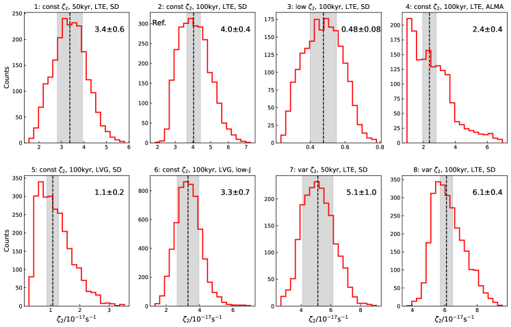
Figure 1: Histogram of the distribution of $\zeta_{2}$ (in units of $10^{-17}\,\rm s^{-1}$) of the runs as labelled at the top of each panel. We represent the core region where $N({\rm H_{2}})>0.5\times\text{max}(N({\rm H_{2}}))$ (i.e. the lowest contour in the panels of Figs. 2, 3, and 4). The median value, together with the median uncertainty, is reported in the top-right corner of each panel and shown as a vertical dashed line with a grey-shaded area. Cf. Table 1.

4 Resulting $\zeta_{2}$ maps

We now apply the analytical expressions described in Sect. 2 to infer the $\zeta_{2}$ maps. Uncertainties on derived quantities are computed pixel-per-pixel assuming standard error propagation calculated from the uncertainties on the column densities that are considered independent. We neglect, for instance, any source of uncertainty from the reaction rates. Once the errors are computed, we mask pixels where the signal-to-noise ratio is $\rm S/N\leq 3$.

4.1 The Bovino et al. (2020) method

To test the analytical method of Bovino et al. (2020, BFL20), we computed $\zeta_{2}$ in the eight runs described in Table 1, varying the $\zeta_{2}$ model (constant or variable), the type of radiative transfer (LTE or LVG), the post-processing method (single-dish or ALMA-like), and the frequency of the molecular lines. All the simulations are isothermal at $15\,\rm K$, and, therefore, the rate coefficient in Eq. (1) is $k_{\mathrm{CO}}^{\mathrm{oH_{3}^{+}}}=2.3\times 10^{-9}\,\rm cm^{3}\,s^{-1}$.

In the following subsections, we discuss in detail the results of each run, showing the obtained $\zeta_{2}$ maps. In order to compare these values with the actual ones, we make use of the $\zeta_{2}$ distributions in Fig. 1. Its panels show the histograms of the ionisation rate values extracted in the densest region of the core (i.e. where the H₂ column density is higher than 50% of its peak value), where the signal-to-noise ratio is higher. The medians of the distributions (vertical dashed lines) are directly compared with the actual value of $2.5\times 10^{-17}\,\rm s^{-1}$ in the runs with constant $\zeta_{2}\rm^{s}$. In runs with variable $\zeta_{2}\rm^{s}$, we compare pixel-by-pixel the ratio between actual and retrieved values, as discussed in Sect. 5.

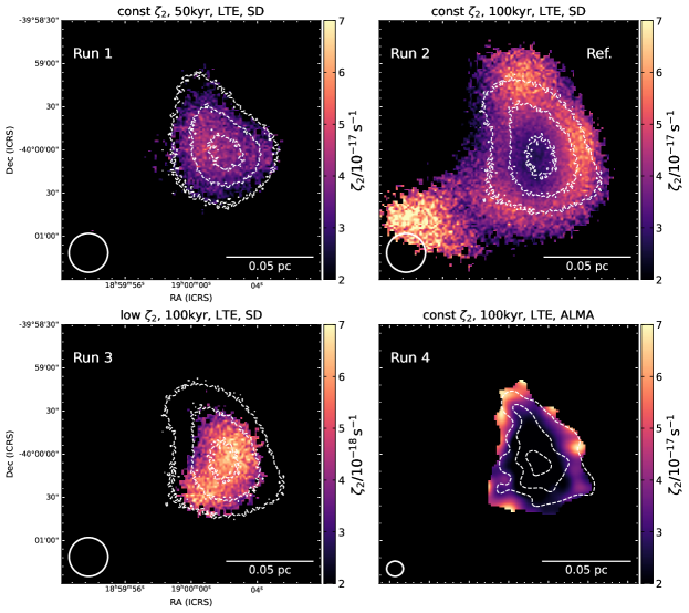
Figure 2: Resulting $\zeta_{2}$ maps (in units of $10^{-17}\,\rm s^{-1}$) obtained with Eq. (1) in runs 1 to 4. The run ID is reported in the top-left corner, and the key parameters are included at the top of each panel. Run 2 is taken as a reference throughout the rest of this work. The white contours show the 50, 70, and 90% of the $N\rm(H_{2})$ peaks, which are: $6.67\times 10^{22}\,\rm cm^{-2}$ (core in single-dish like analysis at 100 kyr); $6.86\times 10^{22}\,\rm cm^{-2}$ (core in single-dish-like analysis at 50 kyr); $2.51\times 10^{22}\,\rm cm^{-2}$ (core in ALMA-like analysis at 100 kyr). The beam size and scalebar are shown in the bottom corners of each panel. Note that we show a zoom-in of the central $0.15\,\rm pc$.

4.1.1 Runs 1-2: constant $\zeta_{2}\rm^{s}$ and single-dish like analysis

The first runs we test have constant $\zeta_{2}^{\mathrm{s}}=2.5\times 10^{-17}\,\rm s^{-1}$, coupled with LTE radiative transfer of the high-J transitions and single-dish-like analysis. We explored two evolutionary stages, 50 kyr (run 1) and 100 kyr (run 2, the reference run). The resulting $\zeta_{2}$ maps are shown in Fig. 2, top row. We employ Eq. (1) with $L=0.3$ pc, which represents the path length (along the line of sight) over which the column densities are integrated. In our case, this corresponds to the size of the simulated box ($\rm 0.3\,pc\times 0.3\,pc\times 0.3\,pc$). A detailed discussion on how to choose $L$ and the derived uncertainty is presented in Sect. 4.3 and 5.

The obtained $\zeta_{2}$ values span the range $\approx(2-8)\times 10^{-17}\,\rm s^{-1}$, with medians in the denser parts of the core of $\zeta_{2}={(3.4\pm 0.6)}\times 10^{-17}\,\rm s^{-1}$ (50 kyr) and $\zeta_{2}=(4.0\pm 0.4)\times 10^{-17}\,\rm s^{-1}$ (100 kyr), as shown in Fig. 1. These values should be compared with the actual $\zeta_{2}^{\mathrm{s}}=2.5\times 10^{-17}\,\rm s^{-1}$. We conclude that, in these runs, the BFL20 reproduces the $\zeta_{2}\rm^{s}$ within a factor $1.5-1.6$ on average.

Concerning the morphology of the retrieved $\zeta_{2}$ maps, the one at $50\,\rm kyr$ shows a smaller scatter around the median value than the run at 100 kyr (see Fig. 1), mainly because we can infer $\zeta_{2}$ only for positions where $N\rm(H_{2})>4.8\times 10^{22}\,\rm cm^{-2}$. This is because at this early stage, the o$\rm H_{2}D^{+}$ abundance is at most $X(\text{o$\rm H_{2}D^{+}$})=7\times 10^{-11}$, producing a line peak intensity of $0.5\,\rm\,K$. For comparison, at 100 kyr, the o$\rm H_{2}D^{+}$ abundance reaches $4\times 10^{-10}$, and the transition is as bright as $3\,\rm K$. This limits the area where $\zeta_{2}$ is computed with $\rm S/N>3$ in run 1.

The histogram from run 2 spans a larger range of values than run 1 and presents a tail at higher values, because the retrieved $\zeta_{2}$ map presents an increase with increasing distance from the core centre, especially in the northern and western directions (cf. top-right panel of Fig. 2). A further enhancement up to $\zeta_{2}\sim 9\times 10^{-17}\,\rm s^{-1}$ is visible in the south-eastern part of the source (note that this does not affect the histogram, which focuses on the high H₂ column density region to improve the $\rm S/N$). In Sect. 5 we discuss more in detail the implication of the spatial trends seen in the $\zeta_{2}$ maps.

4.1.2 Run 3: low $\zeta_{2}\rm^{s}$ and single-dish like analysis

To further expand the range of input $\zeta_{2}\rm^{s}$ values explored and to be consistent with the tests performed by Bovino et al. (2020), we analysed an additional simulation where the $\zeta_{2}$ is kept constant on the value $2.5\times 10^{-18}\,\rm s^{-1}$ (low $\zeta_{2}\rm^{s}$ case). We consider the evolutionary time of $100\,\rm kyr$. The radiative transfer is performed as described in Sect. 3.3, adopting LTE conditions and focusing on the high-J transitions. The post-processing is single-dish-like, with a convolution beam size of $27^{\prime\prime}$. The setup, hence, is identical to the reference run n. 2 except for the input $\zeta_{2}\rm^{s}$ value and the injected noise level. With this $\zeta_{2}\rm^{s}$ value, the deuteration process is slow, and the abundances of deuterated species ($\rm H_{2}D^{+}$, $\rm DCO^{+}$) at $100\,\rm kyr$ are orders of magnitudes lower than in the tests with $\text{$\zeta_{2}\rm^{s}$}=10^{-17}-10^{-16}\rm s^{-1}$. We reduce the simulated noise level to $rms=1\,\rm mK$ in the post-processing, to compute the column density of all species significantly.

Using the BFL20 method, we obtain the map shown in the bottom-left panel of Fig. 2. The corresponding histogram of the distribution of values is shown in Fig. 1. The computed values are in the range $(2-8)\times 10^{-18}\rm\,s^{-1}$, and the median value of $(4.8\pm 0.8)\times 10^{-18}\rm\,s^{-1}$ is less than a factor of two higher than the input $\zeta_{2}\rm^{s}$.

4.1.3 Run 4: ALMA-like analysis

We now focus on the case with constant $\zeta_{2}^{\mathrm{s}}=2.5\times 10^{-17}\rm\,s^{-1}$ and an ALMA-like post-processing as described in Sect. 3.4.2. It is important to discuss the chosen value of $L$. In the single-dish-like analysis, the integrated intensity (or optical depth) is computed along the whole simulated line of sight, i.e. along the whole length of the simulation box (0.3 pc). In the ALMA-like analysis, on the other hand, this is not the case. Once the simobserve task is run, the interferometer acts as a low spatial-frequency filter, and the emission over scales larger than the so-called maximum recoverable scale ($\theta_{\mathrm{mrs}}$) is filtered out. We hence select the $\theta_{\mathrm{mrs}}=15^{\prime\prime}$ that the ALMA OT predicts for the chosen antenna configuration in the o$\rm H_{2}D^{+}(1_{1,0}-1_{1,1})$ setup. This corresponds to $L=0.15\,\rm pc$.

The resulting $\zeta_{2}$ maps is shown in the bottom-right panel of Fig. 2. The histogram of run 4 (top-right panel of Fig. 1) is asymmetric, with a global maximum at low $\zeta_{2}$ values ($1\times 10^{-17}\,\rm s^{-1}$), and a tail up to $7\times 10^{-17}\,\rm s^{-1}$. This is due to the spatial gradient seen in the bottom-right panel of Fig. 2, where $\zeta_{2}$ increases as $N\rm(H_{2})$ decreases. In the central part of the core, the actual $\zeta_{2}\rm^{s}$ is well recovered, as confirmed by comparing the median value ${\langle\zeta_{2}\rangle=(2.4\pm 0.4)\times 10^{-17}\,\rm s^{-1}}$ with $\zeta_{2}^{\mathrm{s}}=2.5\times 10^{-17}\,\rm s^{-1}$.

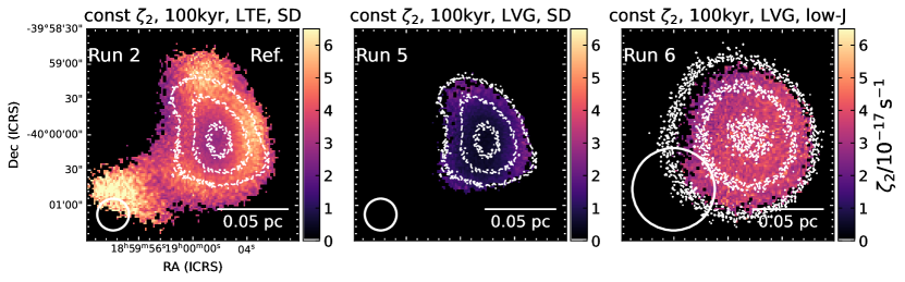
Figure 3: Summary of runs performed in LVG approximation, compared with the reference case (run 2, left panel). The central panel refers to the analysis performed on the high-J transitions for $\rm DCO^{+}$, $\rm H^{13}CO^{+}$, and $\rm C^{18}O$, whilst the low-J ones are used in the map in the right panel. The white contours are the same as in Fig 2. Note that the colour scale is the same across all the panels. The beam size and scalebar are shown in the bottom left and right corners of each panel.

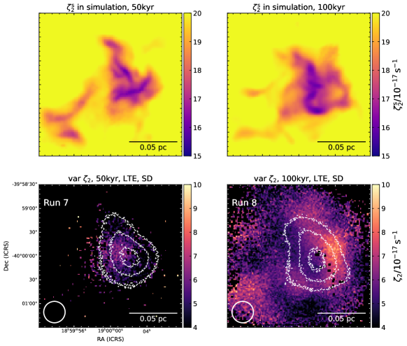
Figure 4: Top row: maps of the density-averaged $\zeta_{2}\rm^{s}$ in the simulation with variable cosmic rays, at 50 kyr (left) and 100 kyr (right). Bottom row: same as Fig. 2, but for runs 7 and 8. Note the colour scale is the same within rows, but it changes from the top panels to the bottom ones.

4.1.4 Runs 5-6: LVG radiative transfer and low-J transition

Runs 5 and 6 explore the effects of the type of radiative transfer performed and of the rotational levels of the lines used in the analysis. Both runs use the LVG option in polaris. Run 5 employs the $\rm DCO^{+}$, $\rm H^{13}CO^{+}$, and $\rm DCO^{+}$ transitions at frequencies $\approx 215-260\,\rm GHz$. The line intensities are generally lower than in the corresponding LTE calculation. The change is the smallest for the $\rm C^{18}O$ (2-1) line ($\approx 15\%$), which is expected as this transition is thermalised. On the contrary, the $\rm DCO^{+}$ and $\rm H^{13}CO^{+}$ (3-2) fluxes are reduced by a factor of up to 3 and 10, respectively. In fact, due to their high critical densities, these transitions are subthermally excited. This requires reducing the simulated noise in this run to 50 mK, to improve the final S/N. Table 2 reports the excitation temperatures used to compute the column densities, following what is stated in Sect. 3.5.

The resulting $\zeta_{2}$ map is shown in the central panel of Fig. 3, and it spans values in the range $(0.5-2.5)\times 10^{-17}\,\rm s^{-1}$. The median in the high-density part of the core (see Fig. 1) is $\langle\zeta_{2}\rangle=(1.1\pm 0.2)\times 10^{-17}\,\rm s^{-1}$, hence a factor $2.3$ smaller than the actual $\zeta_{2}\rm^{s}$ value of the simulations. The $\zeta_{2}$ distribution is asymmetric, as a consequence of the increasing trend of $\zeta_{2}$ with decreasing $N\rm(H_{2})$ that has also been noted in the previous runs at 100 kyr.

In run 6, we explore the effect of targeting the low-J transitions of $\rm C^{18}O$, $\rm H^{13}CO^{+}$, and $\rm DCO^{+}$, as these lines are often targeted by spectroscopic surveys at $3\,$mm. We adopt a large beam size of $\approx 70^{\prime\prime}$, to simulate unresolved observations. The resulting $\zeta_{2}$ map, shown in Fig. 3, presents the flattest distributions of values, with the smallest scatter around the median (see Fig. 1). This happens because the area where we recover the $\zeta_{2}$ map is comparable to the beam size, and hence any spatial trend is smoothed out by the poor resolution. The resulting median $\langle\zeta_{2}\rangle=(3.3\pm{0.7})\times 10^{-17}\,\rm s^{-1}$ agree with the actual $\zeta_{2}\rm^{s}$ $=2.5\times 10^{-17}\,\rm s^{-1}$ within a factor of $1.3$.

4.1.5 Runs 7-8: variable $\zeta_{2}\rm^{s}$

Runs 7 and 8 employ a variable $\zeta_{2}\rm^{s}$, as described in Sect. 3.1. In this case, it is not straightforward to compare the resulting $\zeta_{2}$ maps with the simulation value, which is a three-dimensional, spatially-dependent quantity. For this comparison, we compute the line-of-sight density-averaged $\zeta_{2}\rm^{s}$ at timesteps 50 and 100 kyr. The results are shown in the top row of Fig. 4. The maps show that the cosmic-ray ionisation rate decreases from $\approx 2\times 10^{-16}\,\rm s^{-1}$ at low densities down to $\approx 1.5\times 10^{-16}\,\rm s^{-1}$ in the core’s centre, with a variation of 25%. Moreover, the average value in these simulations is almost one order of magnitude larger than in those with constant $\zeta_{2}$, offering us the chance to test a high $\zeta_{2}$ case.

The maps of $\zeta_{2}$ computed using Eq. (1) are shown in Fig. 4 (bottom panels). In general, they tend to underestimate the simulation values, and the disagreement is larger at the earlier timestep. Overall, our results underestimate the actual $\zeta_{2}\rm^{s}$ of a factor $\approx 3$. Concerning the decrease of $\zeta_{2}$ with increasing total column density, we note that at 50 kyr the extension of the retrieved $\zeta_{2}$ map corresponds to only a few beams, and no clear spatial trend is seen. In the later timestep, a positive gradient is visible from the core’s centre to the westernmost outskirts, but no symmetric trend is visible in the other directions. A localised enhancement ($\zeta_{2}=7-9\times 10^{-17}\,\rm s^{-1}$) is seen in the south-east corner of the source, with no clear counterpart in the actual $\zeta_{2}\rm^{s}$ map, where instead a local decrease is visible in this area. We conclude that the resulting $\zeta_{2}$ map does not reproduce the morphology of the actual one, as we further discuss in Sect. 5.2, but provides an accurate average estimate of $\zeta_{2}\rm^{s}$. In addition, we note that the $\zeta_{2}\rm^{s}$ gradient in the original simulations is smaller than the intrinsic error of the analytical formula.

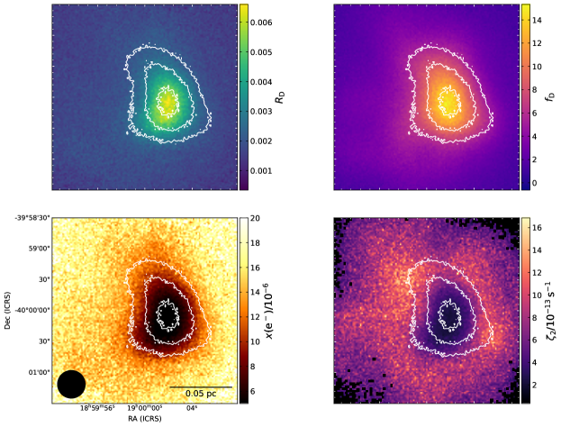
Figure 5: Maps of the key quantities employed by CWT98: $\rm DCO^{+}$ deuteration level (top-left panel), CO depletion factor (top-right), electronic fraction (bottom-left), and $\zeta_{2}$ (bottom-right). Note that the colour scales for the last two quantities are in units of $10^{-6}$ and $10^{-13}\,\rm s^{-1}$, respectively. These maps assume the molecular column density and total gas column density derived in run 2. The mean uncertainties are $2.6\times 10^{-4}$ ($R_{\mathrm{D}}$), $0.3$ ($f_{\mathrm{D}}$), $3\times 10^{-6}$ ($x_{\mathrm{e^{-}}}$), and $1.5\times 10^{-13}\,\rm s^{-1}$ ($\zeta_{2}$). The beam size and scalebar are shown in the bottom-left panel. The contours show $N\rm(H_{2})$, as in Fig. 2.

4.2 The Caselli et al. (1998) analytical method

We now focus on the analytical method proposed by Caselli et al. (1998, CWT98 hereon) to test the limitations already discussed in Caselli et al. (2002), providing robust evidence via an accurate methodology. The CWT98 approach has the advantage of depending on commonly observed tracers. Note that the equations depend on the H₂ volume density, which we estimate as $n(\mathrm{H_{2}})=N(\mathrm{H_{2}})/L$, where $L$ is set on the same value used for the BFL20 method for each run.

4.2.1 The reference run 2

For the sake of observational applicability, we have tested the behaviour of the original equations (Eq. 3 and 4 of CWT98). Here, we present the results for our reference case (run 2). In Fig. 5, we show the relevant required quantities, in particular, the deuteration level of $\rm HCO^{+}$ (top left panel), and the CO depletion factor

$$f_{\mathrm{D}}=\frac{X^{\rm st}(\mathrm{CO})}{X(\mathrm{CO})}\;,$$

where $X^{\rm st}(\mathrm{CO})=1.2\times 10^{-4}$ is the CO standard abundance. The $\rm HCO^{+}$ deuteration level peaks at $R_{\mathrm{D}}={(6.9\pm 0.3)}\times 10^{-3}$ towards the core’s centre, where the CO depletion reaches $f_{\mathrm{D}}={(15.8\pm 0.6)}$. Hence, the deuteration level is smaller than the values spanned by the cores of CWT98, but it fulfils the requirement $R_{\mathrm{D}}<0.023f_{\mathrm{D}}$ under which the equations can be applied. We further discuss this in Sect. 5. The derived values for the electronic fraction, shown in the bottom-left panel, are in the range $(1-10)\times 10^{-6}$. These are overestimated by more than two orders of magnitude compared to the original simulations, where $x(\mathrm{e^{-}})\approx\text{a few}\times 10^{-8}$. This error propagates to the resulting $\zeta_{2}$ map (bottom-right panel of Fig. 5). The equation overestimates the original $\zeta_{2}\rm^{s}$ value by more than three orders of magnitudes, especially at the core’s outskirts.

The original method made several simplifications and assumptions, such as, for example, the reaction rates at constant temperature (10 K), and the lack of ortho- and para-state separation. Furthermore, several reaction rates have been updated since then. We have, therefore, derived the equations again using the same theoretical approach of CWT98, but with the formalism of BFL20, to show that the large overestimates produced by the method are not ascribed to these parameters but rather to the approximations made to obtain the formula. The derivation is illustrated in Appendix B. We have then computed the electronic fraction and the cosmic-ray ionisation rate using the updated set of equations (16). We set the HD abundance to $X(\rm HD)=1.5\times 10^{-5}$ (Kong et al., 2015), and the para-fraction of H${}_{3}^{+}$ to $f_{\mathrm{para}}=0.7$. The latter is consistent with estimates of this parameter in diffuse clouds (see e.g., Crabtree & McCall 2012, and references therein). These values have also been verified in the simulation, and they agree within less than a factor of two (see also Lupi et al. 2021).

The resulting maps are shown in Fig. 6. Towards the core’s centre, the $x(\rm e^{-})$ values are 15-20% lower than those derived with the original equations, but still strongly overestimated. As a consequence, in this area, the new estimates for $\zeta_{2}$ are a factor of $\approx 2$ lower than those from the original derivation, but we still find $\zeta_{2}\approx(1.5\pm{0.2})\times 10^{-13}\rm s^{-1}$, i.e. more than three orders of magnitude higher than the actual value.

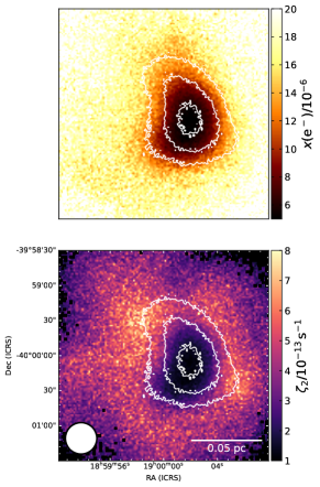
Figure 6: Electronic fraction (top panel) and $\zeta_{2}$ map (bottom panel) from the reference run 2, using the updated formulation of CWT98. The contours show H₂ column density as in Fig. 2. The mean uncertainties are $\mathbf{3}\times 10^{-6}$ for $x(\mathrm{e^{-}})$ and ${0.8}\times 10^{-13}\,\rm s^{-1}$ for $\zeta_{2}$. The beam size and scalebar are shown in the bottom corners of the lower panel.

4.2.2 CWT98 results in all tested runs

We now describe the behaviour of the CWT98 method applied to all the remaining runs. We adopt the new formulation of the method, described in Appendix B. The histograms of the resulting maps, focussing on the central part of the core, are presented in Fig. 7. The most notable feature is that in all tests the retrieved values overestimate the actual ones. The median values in the runs performed on the simulation using $\zeta_{2}^{\mathrm{s}}=\text{cost}=2.5\times 10^{-17}\,\rm s^{-1}$ range from $(4.8\pm 1.4)\times 10^{-15}\,\rm s^{-1}$ (run 5) to $(9.7\pm 1.5)\times 10^{-13}\,\rm s^{-1}$ (run 1), i.e. an overestimation of two to four orders of magnitude. In the low $\zeta_{2}$ case (run 3), we obtain $\langle\zeta_{2}\rangle=(1.41\pm 0.07)\times 10^{-11}\,\rm s^{-1}$ (overestimated by almost seven orders of magnitude). The two tests performed on simulations with $\zeta_{2}^{\mathrm{s}}=\text{var}\approx 10^{-16}\,\rm s^{-1}$ result in $(1.68\pm 0.11)\times 10^{-13}\,\rm s^{-1}$ (run 7) and $(3.1\pm 0.2)\times 10^{-14}\,\rm s^{-1}$ (run 8), again overestimating the actual $\zeta_{2}$ by two-three orders of magnitude.

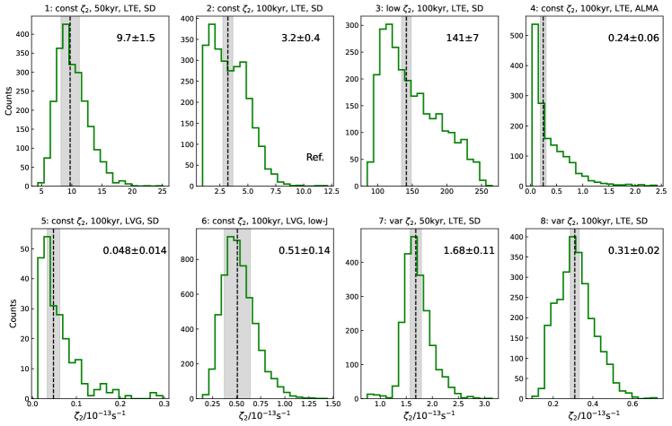
Figure 7: Same as Fig. 1, but the ionisation rate is estimated using the new formulation of the CWT98 method presented in Appendix B, summarised in Eq. (16). Note that the $\zeta_{2}$ values are normalised to $10^{-13}\,\rm s^{-1}$ in all panels. The median ($\pm$ median uncertainty) is reported in the top-right corner and shown with the vertical dashed line and shaded area in each panel.. The reference run is labelled with “Ref” in the bottom-right corner.

4.3 Comparison of the methods on real observations

We now compare the two analytical methods on real observations of prestellar cores found in the literature. We found three sources for which all the needed observables are available: L1544, L183, and TMC-1C. The literature values of the required quantities are listed in Table 4. For these cores, the H₂ volume density is well characterised, and we used this quantity directly in the CWT98 equation  (16). For the BFL20 method, a discussion on the parameter $L$ is required. The physical meaning of $L$ is the length of the path on the line-of-sight along which the column densities are computed; in other words, $L$ is the depth of the emitting source. This, in the simulations, is known by construction. In our setup, we cut a $(0.3\,\rm pc)^{3}$ subcube in the initial larger simulation box (0.6 pc) which is initialised with molecular gas, hence full of e.g. CO. Emitting gas, therefore, is found along the whole box, and the choice of $L$ to be equal to the size of the subcube is well justified. If we were to cut a smaller subcube, $L$ should be adjusted accordingly, since the depth of the emitting gas would also be reduced (see also Appendix D) for further details). This does not apply to real observations. Real cores are finite, and the length of the emitting gas is limited along the length of the line of sight. $L$ hence has to be computed as the source size along the line of sight, which however is completely unknown. For isolated prestellar cores, we propose to compute $L$ by considering the 20% isocontour of the $N\rm(H_{2})$ peak. Using this prescription, the sizes of the three analysed cores are $0.20-0.35\,\rm pc$. The final $\zeta_{2}$ values are also reported in Table 4.

Table 4: Comparison of $\zeta_{2}$ values obtained with the CWT98 and BFL20 methods towards three prestellar cores, assuming a gas temperature of $10\,$K. The reaction rates have been computed at the temperature of $10\,$K.

	$R_{\mathrm{D}}$	$R_{\mathrm{H}}$	$f_{\mathrm{D}}$	$n\rm(H_{2})$	$N\rm(oH_{2}D^{+})$	$L$	$\zeta_{2}$ (CWT98)	$\zeta_{2}$ (BFL20)
	$\times 10^{-2}$	$\times 10^{-5}$		$\times 10^{5}\,\rm cm^{-3}$	$\times 10^{13}\,\rm cm^{-2}$	pc	$\times 10^{-14}\,\rm s^{-1}$	$\times 10^{-17}\,\rm s^{-1}$
L1544	$3.5^{a}$	$5.9^{e}$	$14^{f}$	$14^{g}$	$3.2^{h}$	0.20	$2.0$	$1.0$
L183	$5.1^{b}$	$2.3^{e}$	$12^{g}$	$10^{g}$	$2.5^{h}$	0.20	$0.2$	$0.7$
TMC-1C	$1.6^{c,d}$	$2.8^{d}$	$3^{c}$	$4.5^{d}$	$0.9^{h}$	0.35	$1.2$	$1.7$

The $\zeta_{2}$ values computed with BFL20 are in the range $(0.7-1.7)\times 10^{-17}\,\rm s^{-1}$, whilst with CWT98 we obtain $(0.2-2.0)\times 10^{-14}\,\rm s^{-1}$. Note that there are many uncertainties in the analysis. For instance, the literature values have been computed with data from different telescopes (hence at different resolutions). Furthermore, we assume $T=10\,\rm K$, whilst some of the sources might be colder (cf. Caselli et al., 2008). However, the uncertainties on these quantities cannot explain a difference of three orders of magnitude between the two methods. These examples, hence, confirm that CWT98 tends to produce overestimated results compared to BFL20.

The actual $\zeta_{2}$ value in these objects is not known, however Redaelli et al. (2021b) derived $3.0\times 10^{-17}\,\rm s^{-1}$ in L1544, and Fuente et al. (2019) found $\zeta_{2}=(5-18)\times 10^{-17}\,\rm s^{-1}$ in the translucent cloud associated with TMC1. Both papers used extensive modelling of the sources, coupling chemical models with radiative transfer analysis on a large set of molecular tracers. Pagani et al. (2009) explored the chemistry and structure of L183, assuming ionisation rates in the range $(0.1-10)\times 10^{-16}\,\rm s^{-1}$ and, even though a definite best-value for this parameter is not given, the authors used $\zeta_{2}=2\times 10^{-17}\rm\,s^{-1}$ in their most detailed modelling. Furthermore, the most recent models of CR propagation in the dense gas predict $\zeta_{2}$ values of at most a few $10^{-16}\rm s^{-1}$, unless a local source of CR re-acceleration is present (cf. Padovani et al., 2016, 2018, 2022). It is safe to assume, in summary, that values as high as $\zeta_{2}=10^{-14}\,\rm s^{-1}$ are excluded for these quiescent and dense cores.

5 Discussion

5.1 Results and limitations of the methods

In Fig. 8, we summarise the results obtained with the BFL20 method in the eight runs of Sect. 4.1. In the case of constant $\zeta_{2}\rm^{s}$, we show the average ratio between the derived values and the reference $\zeta_{2}^{\mathrm{s}}=2.5\times 10^{-17}\rm s^{-1}$ (runs 1, 2, and 4 to 6) or $\zeta_{2}^{\mathrm{s}}=2.5\times 10^{-18}\rm s^{-1}$ (run 3). For runs 7 and 8, where the input $\zeta_{2}\rm^{s}$ is variable, we show the median of the ratio between the derived values and the input values (see top panels of Fig. 4). Error bars are computed as three times the median uncertainties over the pixels considered to evaluate the median. As fo the histograms in Fig. 1, we consider only the densest part of the core.

Fig. 8 shows that the retrieved values are within a factor of $1.5-3$ from the actual ones. The offset is not constant, nor systematic. In the cases with low and constant $\zeta_{2}\rm^{s}$, Eq. (1) overestimate the input value by a factor of up to $1.5$ (except run 5). On the other hand, for the two runs with variable $\zeta_{2}\rm^{s}$ (runs 7 and 8), the resulting $\zeta_{2}$ maps tend to underestimate the actual values by a factor of $\approx 3$. Overall, the BFL20 formula represents a robust and reliable method to estimate the order of magnitude of $\zeta_{2}$ in dense regions. As for similar analytical methods, even if the BFL20 method shows to be accurate within a factor of 2-3, several aspects should be taken into account when it is applied to actual observations. The first one is that the analytic expression depends on the column density of four molecular tracers. If any of these is affected by a systematic error, this will propagate to the $\zeta_{2}$ estimation. Column densities strongly depend on the chosen excitation temperature values. By performing an LTE analysis, we have initially avoided this problem, fixing the $T_{\mathrm{ex}}$ for all the molecular tracers to the constant gas temperature. In the LVG runs, we selected $T_{\mathrm{ex}}$ looking for literature references and checking the selected values with non-LTE tools (such as radex). Indirectly, this work hence provides good estimates of the $T_{\mathrm{ex}}$ of several commonly observed transitions, in the considered density ($n\approx 10^{5}\rm cm^{-3}$) and gas temperature ($T_{\mathrm{K}}=15\,\rm K$) regimes. In reality, the problem of choosing the correct $T_{\mathrm{ex}}$ has no straightforward solution, especially in the case of subthermally-excited lines. We strongly suggest, when possible, using multiple lines of the same tracer, which allows us to constrain their excitation conditions better.

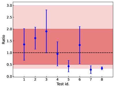
Figure 8: Ratio between $\zeta_{2}$ retrieved in each run ($x$-axis labels), and the actual value $\zeta_{2}\rm^{s}$. The ratios are median computed in each map, in the same regions used to produce the histograms of Fig. 1. The shaded areas show a variation of a factor of 2 (darker shade) or 3 (lighter shade). The dashed line represents where the ratio is equal to 1. The error bars are 3$\sigma$ median uncertainties.

When using optically-thin isotopologues to infer the total column densities of molecular tracers, particular caution has to be paid to the assumed isotopic ratios, since fractionation processes can lead to significant variation from the elemental isotopic ratios (see, e.g., the discussion of Colzi et al. 2020 on $\rm{}^{12}C/^{13}C$). In this work, we avoided this problem by assuming consistent isotopic ratios throughout the postprocessing analysis (cf. Sects. 3.1 and 3.3).

Another crucial parameter in Eq. (1) is the scale length $L$ employed to obtain the column densities, as discussed in Sect. 4. In our analysis, $L$ is known by construction from the size of the simulation box, since this is a subcube cut out of a larger simulation initialised with molecular gas. We justify this choice further in Appendix D. For observed cores, their size (and, in particular, their depths) are in general unknown. We suggest as a prescription to use the contour where $N\rm(H_{2})$ is higher than 20% of its peak value to estimate $L$. In the three real objects we analysed, this approach leads to $\zeta_{2}$ values in agreement with estimations of this quantity derived with completely different methods. Note that applying this rule to the reference run 2 results in $L=0.15$ pc, hence overestimating $\zeta_{2}$ by a factor $\approx 2$, still within the uncertainties of the method. This prescription should not be used on interferometric data with a maximum recoverable scale smaller than the actual source size, as this leads to emission filtering. In these cases, we speculate that $\theta_{\mathrm{mrs}}$ is a proper scale to estimate $L$. This uncertainty on $L$ also affects the approach of CWT98, where however this is mitigated if the gas volume density is known from other observables.

We highlight how the core fraction where we are able to infer $\zeta_{2}$ is different in each case (see Figs. 2, 3, and 4). This is driven, in particular, by the column density of o$\rm H_{2}D^{+}$. At earlier times, the abundance of this species is lower, hence the extension of the core where it is detected is smaller. This highlights the main limitation of this method, i.e. that it relies on the detection of o$\rm H_{2}D^{+}(1_{1,0}-1_{1,1})$ (see also Sect. 5.3 for details).

On the other hand, the analytic method of CWT98 overestimates $\zeta_{2}$ by several orders of magnitudes in the cases explored in this work, where it should not be employed (see also the discussion in Sect. 3 of Caselli et al. 2002). This is due to the overestimation of the electron fraction caused by the neglected kinetics of $\rm H_{2}D^{+}$ employed to derive Eq. (12), in particular, the reactions producing the doubly- and triply-deuterated forms of H${}_{3}^{+}$, and other destruction channels involving neutrals. Concerning the importance of $\rm D_{2}H^{+}$ and D${}_{3}^{+}$, Caselli et al. (2008) developed analytical equations where the deuteration level of $\rm HCO^{+}$ is expressed in terms of all the deuterated forms of H${}_{3}^{+}$.

Note that $\zeta_{2}$, when derived in the reference case with the analytic expression of CWT98 ($10^{-14}-10^{-13}\rm\,s^{-1}$), is one to two orders of magnitude higher than in the original paper (where $\zeta_{2}=10^{-16}-10^{-14}\rm\,s^{-1}$ was found when assuming $f_{\mathrm{D}}=5$). This is because the simulated core presents relatively low levels of deuteration and a high depletion factor. In Appendix B, we show how the CWT98 formula leads to increasingly high $\zeta_{2}$ values when the deuteration is low, and the CO depletion is high (cf. Fig. 10). In the reference case (run 2), the core centre presents $R_{\mathrm{D}}\approx 0.4-0.7$% and $f_{\mathrm{D}}\approx 10-15$. These are not the typical values observed in CWT98, where most sources present a deuteration fraction of a few per cent (see also Butner et al., 1995; Williams et al., 1998). Note that, given the lack of information available back then on the CO depletion, $f_{\mathrm{D}}>5$ was not included in their analysis (catastrophic CO freeze-out was first measured one year later, Caselli et al. 1999). Furthermore, the assumed temperature $T=15\,\rm K$ is higher than typical gas temperatures observed in low-mass prestellar cores (Bergin et al., 2006; Crapsi et al., 2007). However, in run 8, with variable $\zeta_{2}$ at 100 kyr, the core’s centre presents $R_{\mathrm{D}}\approx 2$% and $f_{\mathrm{D}}\approx 3-4$, closer to the properties of the objects analysed by CWT98. The retrieved $\zeta_{2}$ is $(3.1\pm 0.2)\times 10^{-14}\,\rm s^{-1}$ (see Fig. 7), overestimating the actual $\zeta_{2}\rm^{s}$ by two orders of magnitudes, confirming the limitation of this approach.

The relatively low deuteration level of the reference case is due to the assumed initial conditions, in particular the initial H₂ OPR. By using constant-density one-zone models, we foundthat when $\text{OPR}=10^{-3}$ (as reported in the dense and evolved prestellar cores, e.g. Kong et al. 2015), the $\rm HCO^{+}$ deuteration level increases by about one order of magnitude, and the derived $\zeta_{2}$ values decrease to $\zeta_{2}=10^{-16}-10^{-15}\rm\,s^{-1}$, still a factor of 10-100 more than the actual value. These tests show that the CWT98 analytic method has a marked dependence on the initial OPR, conversely to BFL20, which is relatively unaffected by this parameter, as already discussed in Bovino et al. (2020). The scope of this work is to retrieve $\zeta_{2}$ under the typical observational conditions while reproducing the exact physical details of a specific observed object is beyond our aims. The latter was done, for example, by Bovino et al. (2021), where the simulation was designed to reproduce six observed cores in Ophiucus.

5.2 Morphology of the resulting $\zeta_{2}$ maps

The obtained $\zeta_{2}$ maps allow us to comment also on the morphology of the retrieved ionisation rate. By looking at Figs. 2 and 3, it is clear that for most of the runs where $\zeta_{2}$ is computed in an extended part of the source (i.e. when $N\rm(H_{2})\lesssim$50% of its peak), $\zeta_{2}$ presents a positive gradient with increasing distance from the core’s centre. This is also seen in the histograms in Fig. 1, where asymmetric tails towards the high $\zeta_{2}$ values are seen in runs 2, 4, and 5. Since in these runs, the actual $\zeta_{2}\rm^{s}$ is constant, these spatial trends are not real. These considerations holds also for CWT98 (see Figs. 5 and 6). The single-dish test performed with the larger beam size (run 6) presents the flattest distribution and the smallest scatter around the median because the core is not spatially resolved. On the contrary, in the tests with variable $\zeta_{2}\rm^{s}$, the retrieved maps do not show the gradient with the increasing density present in the simulation (see Sect. 4.1.5 for more details). We conclude that apparent spatial trends should not be trusted, and averages across the densest regions of the source should be instead considered to express the resulting $\zeta_{2}$.

5.3 Observational feasibility

This work aims to provide observers with reliable methods to estimate $\zeta_{2}$ in real sources. It is hence important to assess the observability of the proposed tracers. The continuum observations are not particularly challenging and do not represent the limiting aspect of this endeavour. Conversely, the feasibility of the molecular line observations requires a more detailed discussion.

We first focus on single-dish facilities. As reported in Table 2, the $\rm H^{13}CO^{+}$ (3-2), $\rm DCO^{+}$ (3-2), ad $\rm C^{18}O$ (2-1) lines can be observed by APEX, i.e. with the nFLASH230 instrument. Using its observing time calculator, and standard input values, we compute that on-source times of $1.0-1.4\,\rm h$ are sufficient to reach $rms=100\,\rm mK$ in a $3^{\prime}\times 3^{\prime}$ FoV and a 0.1 $\rm km\,s^{-1}$ channel. The corresponding (1-0) transitions are covered, for instance, by the EMIR receiver mounted on the IRAM 30m telescope. The time estimator predicts that, in winter, $1\,$h of on-source time is enough to reach a sensitivity of $100\,\rm mK$, with a $3^{\prime}\times 3^{\prime}$ FoV and using a 0.1 $\rm km\,s^{-1}$ resolution.

The o$\rm H_{2}D^{+}(1_{1,0}-1_{1,1})$ transition is the most challenging in terms of sensitivity, due to its high frequency when compared to the other transitions analysed here. The same requirements in terms of spectral resolution, sky coverage, and sensitivity made for the other lines would lead to $25\,$h of on-source time using the multi-beam LASMA receiver mounted on APEX. However, by relaxing the requirements to a FoV of $2^{\prime}\times 2^{\prime}$ (still able to cover the portion of the core where $N\rm(H_{2})\gtrsim 2.5\times 10^{22}\,cm^{-2}$) and downgrading the resolution to $0.15\,$$\rm km\,s^{-1}$, the on-source time reduces to $7.5\,$h, which is manageable in a small project. The downgraded spectral resolution does not impact the computation of the column density, since the lines are still resolved by at least 3 channels. The sensitivity required by the low $\zeta_{2}$ case in run 3 ($1\,$mK), on the other hand, is currently well beyond the capabilities of existing single-dish facilities, even in the case of single-point observations at the centre of the source.

The observing times required with ALMA are listed in Table 3. Considering that several lines can be observed simultaneously, these observations appear feasible. We conclude that in most cases the observations required to compute $\zeta_{2}$ are feasable, as proved by the increasing number of campaigns recently reported (cf. Giannetti et al., 2019; Sabatini et al., 2020; Redaelli et al., 2021a, 2022).

6 Summary and conclusions

In this work, we have tested two analytical methods to retrieve the cosmic-ray ionization rate $\zeta_{2}$ in dense gas. This has been done using synthetic molecular and continuum data, produced via radiative transfer analysis on a set of three-dimensional simulations that include the chemistry of the involved molecular tracers. This allows us to evaluate with accuracy the loss of information (and then the accuracy of the method) when simulating realistic observations.

The method of Caselli et al. (1998) has several limitations by construction, such as $R_{\mathrm{D}}<0.029\times f_{\mathrm{D}}$ (to avoid $x(\rm e)<0$ in the new formulation derived in Appendix B). Furthermore, this analytical approach strongly depends on the H₂ initial OPR. This limits its applicability, especially when the OPR is reset to much higher values than those in cold cores by conditions such as shocks or protostellar outflows. In our reference case, this method overestimates $\zeta_{2}\rm^{s}$ by up to four orders of magnitude. In particular, in tests where the deuteration level is a few %, hence similar to what is observed in several prestellar cores, the Caselli et al. (1998) method overestimates by two orders of magnitude the actual $\zeta_{2}\rm^{s}$.

On the contrary, the method of Bovino et al. (2020) is generally accurate within a factor of $2-3$ in retrieving the actual $\zeta_{2}\rm^{s}$. Its main limitation is linked to the level of total deuteration, since at late evolutionary stages or at very high densities ($n\gtrsim 10^{7}\,\rm cm^{-3}$) $\rm H_{2}D^{+}$ is converted into doubly and triply deuterated forms, and it is not a reliable tracer of the total $\rm H_{3}^{+}$ abundance anymore. This leads to underestimating the actual $\zeta_{2}\rm^{s}$, as already pointed out in the original paper (Bovino et al., 2020).

As a direct example of the application of the two formulae on observational data, we explored three well-known prestellar objects, with recent literature data on the quantities involved in the calculation. We showed that the $\zeta_{2}$ values obtained with BFL20 are in overall good agreement with estimations of the same quantities obtained with non-analytical methods. The results of CWT98 are two to three orders of magnitude higher, as seen also in the tests on the simulations. We highlight, however, that to establish the methodology proposed by Bovino et al. (2020), a statistical sample of observed cores and a proper comparison with theoretical models of CR propagation are needed.

To conclude, we have discussed the feasibility of the observations necessary to use two commonly employed analytical methods to retrieve $\zeta_{2}$. Despite the observational challenges, they are accessible with currently available radio facilities. When the physical structure of a source is well known, coupling a chemical code with radiative transfer using multiple tracers could be employed to infer the cosmic-ray ionisation rate, even if its results might be affected by the parameters’ degeneracy. For all the other sources (when this approach is not a viable option), the method of Bovino et al. (2020) is a model-independent and reliable analytical method to investigate $\zeta_{2}$ in dense regions.

Appendix A Derivation of Bovino et al. (2020) (BFL20)

We now follow the derivation of Eq. (1). The main reactions in our framework, considering the different isomers and isotopologues (but $\rm D_{3}^{+}$) for the formation of HCO⁺ and DCO⁺ are:

$$\mathrm{oH_{2}D^{+}}+\mathrm{CO}\xrightarrow{{k_{1}}}\rm DCO^{+}+oH_{2}$$

$$\mathrm{pH_{2}D^{+}}+\mathrm{CO}\xrightarrow{{k_{2}}}\rm DCO^{+}+pH_{2}$$

$$\mathrm{pD_{2}H^{+}}+\mathrm{CO}\xrightarrow{{k_{3}}}\rm DCO^{+}+HD$$

$$\mathrm{oD_{2}H^{+}}+\mathrm{CO}\xrightarrow{{k_{4}}}\rm DCO^{+}+HD$$

$$\mathrm{pH_{3}^{+}}+\mathrm{CO}\xrightarrow{{k_{5}}}\rm HCO^{+}+pH_{2}$$

$$\mathrm{pH_{3}^{+}}+\mathrm{CO}\xrightarrow{{k_{6}}}\rm HCO^{+}+oH_{2}$$

$$\mathrm{oH_{3}^{+}}+\mathrm{CO}\xrightarrow{{k_{7}}}\rm HCO^{+}+oH_{2}$$

$$\mathrm{pD_{2}H^{+}}+\mathrm{CO}\xrightarrow{{k_{8}}}\rm HCO^{+}+pD_{2}$$

$$\mathrm{pH_{3}^{+}}+\mathrm{CO}\xrightarrow{{k_{6}}}\rm HCO^{+}+oH_{2}$$

$$\mathrm{oH_{3}^{+}}+\mathrm{CO}\xrightarrow{{k_{7}}}\rm HCO^{+}+oH_{2}$$

$$\mathrm{pD_{2}H^{+}}+\mathrm{CO}\xrightarrow{{k_{8}}}\rm HCO^{+}+pD_{2}$$

$$\mathrm{oD_{2}H^{+}}+\mathrm{CO}\xrightarrow{{k_{9}}}\rm HCO^{+}+oD_{2}$$

$$\mathrm{pH_{2}D^{+}}+\mathrm{CO}\xrightarrow{{k_{10}}}\rm HCO^{+}+HD$$

$$\mathrm{oH_{2}D^{+}}+\mathrm{CO}\xrightarrow{{k_{11}}}\rm HCO^{+}+HD$$

For the destruction, we consider only dissociative recombinations

$$\mathrm{DCO^{+}+e^{-}}\xrightarrow{\beta_{1}}\mathrm{D+CO}$$

$$\mathrm{HCO^{+}+e^{-}}\xrightarrow{\beta_{2}}\mathrm{H+CO}$$

The kinetic equations read as

$$\frac{dn(\mathrm{DCO^{+}})}{dt}=k_{1}n(\mathrm{CO})n(\mathrm{oH_{2}D^{+}})+k_{2}n(\mathrm{CO})n(\mathrm{pH_{2}D^{+}})+k_{3}n(\mathrm{CO})n(\mathrm{pD_{2}H^{+}})+k_{4}n(\mathrm{CO})n(\mathrm{oD_{2}H^{+}})-\beta_{1}n(\mathrm{DCO^{+}})n(\mathrm{e^{-}})$$

and

$$\begin{split}\frac{dn(\mathrm{HCO^{+}})}{dt}=&\;(k_{5}+k_{6})n(\mathrm{CO})n(\mathrm{pH_{3}^{+}})+k_{7}n(\mathrm{CO})n(\mathrm{oH_{3}^{+}})+k_{8}n(\mathrm{CO})n(\mathrm{pD_{2}H^{+}})+k_{9}n(\mathrm{CO})n(\mathrm{oD_{2}H^{+}})\;+\\ &+k_{10}n(\mathrm{CO})n(\mathrm{pH_{2}D^{+}})+k_{11}n(\mathrm{CO})n(\mathrm{oH_{2}D^{+}})-\beta_{2}n(\mathrm{HCO^{+}})n(\mathrm{e^{-}})\,.\end{split}$$

Assuming steady-state and taking the ratio between the two equations we obtain

$$\begin{split}R_{D}&=\frac{n(\mathrm{DCO^{+}})}{n(\mathrm{HCO^{+}})}=\left(\frac{\beta_{2}}{\beta_{1}}\right)\times\\ &\frac{k_{1}n(\mathrm{CO})n(\mathrm{oH_{2}D^{+}})+k_{2}n(\mathrm{CO})n(\mathrm{pH_{2}D^{+}})+k_{3}n(\mathrm{CO})n(\mathrm{pD_{2}H^{+}})+k_{4}n(\mathrm{CO})n(\mathrm{oD_{2}H^{+}})}{(k_{5}+k_{6})n(\mathrm{CO})n(\mathrm{pH_{3}^{+}})+k_{7}n(\mathrm{CO})n(\mathrm{oH_{3}^{+}})+k_{8}n(\mathrm{CO})n(\mathrm{pD_{2}H^{+}})+k_{9}n(\mathrm{CO})n(\mathrm{oD_{2}H^{+}})+k_{10}n(\mathrm{CO})n(\mathrm{pH_{2}D^{+}})+k_{11}n(\mathrm{CO})n(\mathrm{oH_{2}D^{+}})}\;.\end{split}$$

Using the following relations among the reaction rates

• $k_{1}=k_{2}$   ,

• $k_{3}=k_{4}$  ,

• $k_{5}+k_{6}=k_{7}$  ,

• $k_{8}=k_{9}$  ,

• $k_{10}=k_{11}$  ,

• $\beta_{2}=\beta_{1}$  ,

the final equation reads (note that $n(\mathrm{CO})$ and $n(\mathrm{e^{-}})$ cancel out)

$$R_{D}=\frac{n(\mathrm{DCO^{+}})}{n(\mathrm{HCO^{+}})}=\frac{k_{1}\left[n(\mathrm{oH_{2}D^{+}})+n(\mathrm{pH_{2}D^{+}})\right]+k_{3}\left[n(\mathrm{pD_{2}H^{+}})+n(\mathrm{oD_{2}H^{+}})\right]}{k_{7}\left[n(\mathrm{oH_{3}^{+}})+n(\mathrm{pH_{3}^{+}})\right]+k_{8}\left[n(\mathrm{pD_{2}H^{+}})+n(\mathrm{oD_{2}H^{+}})\right]+k_{10}\left[n(\mathrm{pH_{2}D^{+}})+n(\mathrm{oH_{2}D^{+}})\right]}\;.$$ (6)

In order to simplify Eq. (6), we can exploit further relations between the reaction rates, mainly linked to their branching ratios: $k_{1}/k_{7}=1/3$, $k_{1}/k_{10}=1/2$, $k_{8}/k_{3}=1/2$, and $k_{3}/k_{7}=2/3$. Moreover, we neglect the correction for para and ortho species that cannot be observed, the contribution from the doubly deuterated isotopologue, and the formation channel of $\rm HCO^{+}$ via $\rm H_{2}D^{+}$, arriving at

$$n(\mathrm{H_{3}^{+}})=\frac{1}{3}\frac{n(\mathrm{oH_{2}D^{+}})}{R_{D}}\,.$$ (7)

By inserting Eq. (7) in (see e.g. Oka 2019, and also the derivation in Appendix B)

$$\zeta_{2}=\frac{k_{7}n(\mathrm{H_{3}^{+}})n(\mathrm{CO})}{n(\mathrm{H_{2}})}\;,$$ (8)

we obtain the final formula for the cosmic-ray ionisation rate

$$\zeta_{2}=\frac{1}{3}\frac{k_{7}n(\mathrm{oH_{2}D^{+}})}{R_{D}}\frac{n(\mathrm{CO})}{n(\mathrm{H_{2}})}\;.$$ (9)

This equation is valid as long as o$\rm H_{2}D^{+}$ is the dominant deuterated form of H${}_{3}^{+}$ and when the reaction with CO is more important than dissociative recombination in the destruction of $\rm H_{3}^{+}$. The first limitation implies that when deuteration levels become higher and o$\rm H_{2}D^{+}$ is converted into its doubly and triply deuterated isotopologues, Eq. (9) cannot be used anymore. Concerning the destruction pathways, we can investigate at which CO abundance (as a function of the electronic fraction) its reaction with $\rm H_{3}^{+}$ dominates over the dissociative recombination (see the right-hand side of Eq. (15)). We find that this holds for $f_{\mathrm{D}}<9\times 10^{-7}/x(\mathrm{e^{-}})$ (assuming $f_{\mathrm{para}}=0.7$, see also Appendix B). For $x(\mathrm{e})=10^{-8}$, close to the values found in the reference run, the reaction with CO is dominant if $f_{\mathrm{D}}\lesssim 90$, which is verified in our simulations. However, at very high densities, when $f_{\mathrm{D}}\gtrsim 100$, this assumption might not hold anymore.

By introducing average quantities integrated over the path $L$ along the line of sight, Eq. (9) finally becomes

$$\zeta_{2}=k_{7}\frac{1}{3}\times X(\mathrm{CO})\times\frac{N_{\mathrm{col}}(\mathrm{oH_{2}D^{+}})}{R_{\mathrm{D}}}\frac{1}{L}\;.$$ (10)

Note that $k_{7}=k_{\mathrm{CO}}^{\rm oH_{3}^{+}}$ in the main text.

Appendix B Derivation of Caselli et al. (1998) (CWT98)

We now illustrate the derivation of the equations used in Caselli et al. (1998), which in turn are based on previous works (e.g. Guelin et al. 1977, 1982). In particular, we aim to follow the same approach as those papers, including this time the ortho/para separation for all the involved species.

The first part of the equations is the same as illustrated in Appendix A, and involves balancing the destruction and formation pathways of $\rm HCO^{+}$ and $\rm DCO^{+}$, arriving at (see Eq. (6))

$$R_{D}=\frac{1}{3}\frac{n(\mathrm{H_{2}D^{+}})}{n(\rm H_{3}^{+})}\;,$$ (11)

where we neglect the reactions involving doubly and triply deuterated H${}_{3}^{+}$ and reactions 10 and 11). In this case, however, we look for a way to express the ratio $n(\mathrm{H_{2}D^{+}})/n(\rm H_{3}^{+})$ as a function of the densities of CO, HD, and of the electron fraction. To this aim, we have to write the reactions involved in the formation and destruction of $\rm H_{2}D^{+}$ (in its ortho and para states). For the formation pathways, we have

$$\mathrm{pH_{3}^{+}+HD}\xrightarrow{{k_{12}}}\rm\mathrm{pH_{2}D^{+}}+pH_{2}$$

$$\mathrm{pH_{3}^{+}+HD}\xrightarrow{{k_{13}}}\rm\mathrm{pH_{2}D^{+}}+oH_{2}$$

$$\mathrm{pH_{3}^{+}+HD}\xrightarrow{{k_{14}}}\rm\mathrm{oH_{2}D^{+}}+pH_{2}$$

$$\mathrm{pH_{3}^{+}+HD}\xrightarrow{{k_{15}}}\rm\mathrm{oH_{2}D^{+}}+oH_{2}$$

$$\mathrm{oH_{3}^{+}+HD}\xrightarrow{{k_{16}}}\rm\mathrm{pH_{2}D^{+}}+oH_{2}$$

$$\mathrm{oH_{3}^{+}+HD}\xrightarrow{{k_{17}}}\rm\mathrm{oH_{2}D^{+}}+oH_{2}$$

$$\mathrm{oH_{3}^{+}+HD}\xrightarrow{{k_{18}}}\rm\mathrm{oH_{2}D^{+}}+pH_{2}$$

The destruction pathways, instead, involve the reactions with CO (with rates $k_{1}$, $k_{2}$, $k_{10}$, and $k_{11}$, see above), and the following dissociative recombinations

$$\begin{split}\rm\mathrm{oH_{2}D^{+}}+e^{-}&\xrightarrow{{\beta_{3}}}\rm H+H+D\\ \rm\mathrm{oH_{2}D^{+}}+e^{-}&\xrightarrow{{\beta_{4}}}\rm D+oH_{2}\\ \rm\mathrm{oH_{2}D^{+}}+e^{-}&\xrightarrow{{\beta_{5}}}\rm H+H\\ \rm\mathrm{pH_{2}D^{+}}+e^{-}&\xrightarrow{{\beta_{6}}}\rm H+H+D\\ \rm\mathrm{pH_{2}D^{+}}+e^{-}&\xrightarrow{{\beta_{7}}}\rm D+pH_{2}\\ \rm\mathrm{pH_{2}D^{+}}+e^{-}&\xrightarrow{{\beta_{8}}}\rm H+HD\end{split}$$

Note that we have neglected all the reactions involving doubly and triply deuterated $\rm H_{3}^{+}$, to be consistent with the simplification done to obtain Eq. (11). For several of the involved reaction rates, it is possible to show that

• $k_{12}+k_{13}+k_{14}+k_{15}\approx k_{16}+k_{17}+k_{18}$

• $\beta_{3}\approx\beta_{6}$

• $\beta_{4}\approx\beta_{7}$

• $\beta_{5}\approx\beta_{8}$

These relations do not hold exactly, but we will show that in the temperature range here considered the agreement is reasonably good. The first relation is reported in the left panel of Fig. 9. For temperatures $\lesssim 25\,\rm K$, the discrepancy is lower than 10%, and in the range $10-15\,\rm K$, the difference is $1-3$%. We hence assume that equality holds. For the various rates of dissociative recombination ($\beta_{3}$ to $\beta_{8}$), the difference at $15\,\rm K$ is $\approx 6$%, but it quickly rises above 25% outside the range $10-20\,\rm K$. We hence suggest extreme caution in using these and the following relations outside this temperature range. However, without these assumptions, it is in practice impossible to properly re-derive and upgrade the formula proposed by CWT98.

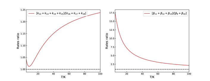
Figure 9: Left panel: the ratio between the sum of the rates of the reactions between $\rm pH_{3}^{+}$ and HD and those involving $\rm oH_{3}^{+}$ and HD, as a function of temperature. Right panel: the ratio between the total rate of dissociative recombination of $\rm pH_{3}^{+}$ and that of $\rm oH_{3}^{+}$, as a function of temperature. In both panels, the horizontal dashed lines correspond to unity.

We can now write the kinetic equations for the para and ortho species separately as

$$\begin{split}\frac{dn(\mathrm{oH_{2}D^{+}})}{dt}&={k}_{14}n(\mathrm{pH_{3}^{+}})n(\mathrm{HD})+{k}_{15}n(\mathrm{pH_{3}^{+}})n(\mathrm{HD})+{k}_{17}n(\mathrm{oH_{3}^{+}})n(\mathrm{HD})+{k}_{18}n(\mathrm{oH_{3}^{+}})n(\mathrm{HD})\\ &-\mathrm{k}_{1}n(\mathrm{\mathrm{oH_{2}D^{+}}})n(\mathrm{CO})-{k}_{11}n(\mathrm{\mathrm{oH_{2}D^{+}}})n(\mathrm{CO})-\beta_{3}n(\mathrm{oH_{2}D^{+}})n(\mathrm{e^{-}})-\beta_{4}n(\mathrm{oH_{2}D^{+}})n(\mathrm{e^{-}})-\beta_{5}n(\mathrm{oH_{2}D^{+}})n(\mathrm{e^{-}})\;,\end{split}$$

and

$$\begin{split}\frac{dn(\mathrm{pH_{2}D^{+}})}{dt}&={k}_{12}n(\mathrm{pH_{3}^{+}})n(\mathrm{HD})+{k}_{13}n(\mathrm{pH_{3}^{+}})n(\mathrm{HD})+{k}_{16}n(\mathrm{oH_{3}^{+}})n(\mathrm{HD})-{k}_{2}n(\mathrm{\mathrm{pH_{2}D^{+}}})n(\mathrm{CO})+\\ &-{k}_{10}n(\mathrm{\mathrm{pH_{2}D^{+}}})n(\mathrm{CO})-\beta_{6}n(\mathrm{pH_{2}D^{+}})n(\mathrm{e^{-}})-\beta_{7}n(\mathrm{pH_{2}D^{+}})n(\mathrm{e})-\beta_{8}n(\mathrm{pH_{2}D^{+}})n(\mathrm{e^{-}})\;.\end{split}$$

Assuming the steady state, we can re-write the two equations above as

$$\begin{split}({k}_{14}+{k}_{15})n(\mathrm{pH_{3}^{+}})n(\mathrm{HD})+({k}_{17}+{k}_{18})n(\mathrm{oH_{3}^{+}})n(\mathrm{HD})&=({k}_{1}+{k}_{11})n(\mathrm{\mathrm{oH_{2}D^{+}}})n(\mathrm{CO})+(\beta_{3}+\beta_{4}+\beta_{5})n(\mathrm{oH_{2}D^{+}})n(\mathrm{e^{-}})\;,\\ ({k}_{12}+{k}_{13})n(\mathrm{pH_{3}^{+}})n(\mathrm{HD})+{k}_{16}n(\mathrm{oH_{3}^{+}})n(\mathrm{HD})&=({k}_{2}+{k}_{10})n(\mathrm{\mathrm{pH_{2}D^{+}}})n(\mathrm{CO})+(\beta_{6}+\beta_{7}+\beta_{8})n(\mathrm{pH_{2}D^{+}})n(\mathrm{e^{-}})\;.\end{split}$$

By summing the two equations above and exploiting the relations between the reaction rates, we arrive at:

$$({k}_{12}+{k}_{13}+{k}_{14}+{k}_{15})n(\mathrm{H_{3}^{+}})n(\mathrm{HD})=({k}_{1}+{k}_{11})n(\mathrm{H_{2}D^{+}})n(\mathrm{CO})+(\beta_{3}+\beta_{4}+\beta_{5})n(\mathrm{H_{2}D^{+}})n(\mathrm{e^{-}})\;,$$

which allows us to rewrite Eq. (11) as

$$R_{\mathrm{D}}=\frac{1}{3}\frac{n(\rm{H_{2}D^{+}})}{n(\rm H_{3}^{+})}=\frac{1}{3}\frac{({k}_{12}+{k}_{13}+{k}_{14}+{k}_{15})n(\mathrm{HD})}{({k}_{1}+{k}_{11})n(\mathrm{CO})+(\beta_{3}+\beta_{4}+\beta_{5})n(\mathrm{e^{-}})}\;.$$ (12)

The next step is to express the quantity $R_{\mathrm{H}}=n(\mathrm{HCO^{+}})/n(\mathrm{CO})$ as a function of the cosmic ray ionisation rate and the electronic fraction. First, we solve the kinetic equation for $\rm HCO^{+}$ in steady-state, again neglecting all terms containing $\rm D_{2}H^{+}$ and D${}_{3}^{+}$ (see above):

$$R_{\mathrm{H}}=\frac{n(\mathrm{HCO^{+}})}{n(\mathrm{CO})}=\frac{k_{7}n(\mathrm{H_{3}^{+}})}{\beta_{2}n(\mathrm{e^{-}})}\;.$$ (13)

To find an expression for $n(\mathrm{H_{3}^{+}})$, we solve its kinetics. Its total formation rate is $\zeta_{2}n(\mathrm{H_{2}})$. The destruction pathways instead are separated in the ortho and para species, and involve the reaction with CO (reactions 5 to 7) and the following dissociative recombinations:

$$\begin{split}\rm oH_{3}^{+}+e^{-}&\xrightarrow{\beta_{9}}\rm H+H+H\\ \rm oH_{3}^{+}+e^{-}&\xrightarrow{\beta_{10}}\rm H+oH_{2}\\ \rm pH_{3}^{+}+e^{-}&\xrightarrow{\beta_{11}}\rm H+H+H\\ \rm pH_{3}^{+}+e^{-}&\xrightarrow{\beta_{12}}\rm H+pH_{2}\\ \rm pH_{3}^{+}+e^{-}&\xrightarrow{\beta_{13}}\rm H+oH_{2}\end{split}$$

The destruction rates of the two species are then:

$$\begin{split}\left.\frac{dn(\mathrm{oH_{3}^{+}})}{dt}\right|_{\mathrm{destr}}&=-\left[k_{7}n(\mathrm{oH_{3}^{+}})n(\mathrm{CO})+\left(\beta_{9}+\beta_{10}\right)(\mathrm{oH_{3}^{+}})n(\mathrm{e^{-}})\right]\;,\\ \left.\frac{dn(\mathrm{pH_{3}^{+}})}{dt}\right|_{\mathrm{destr}}&=-\left[\left(k_{5}+k_{6}\right)n(\mathrm{pH_{3}^{+}})n(\mathrm{CO})+\left(\beta_{11}+\beta_{12}+\beta_{13}\right)(\mathrm{pH_{3}^{+}})n(\mathrm{e^{-}})\right]\;.\end{split}$$

From these equations, we can then compute the destruction rate for the total $\rm H_{3}^{+}$ density, and set it equal to the total formation rate, obtaining:

$$\zeta_{2}n(\mathrm{H_{2}})=k_{7}n(\mathrm{H_{3}^{+}})n(\mathrm{CO})+n(\mathrm{e^{-}})\left[\left(\beta_{11}+\beta_{12}+\beta_{13}\right)n(\mathrm{pH_{3}^{+}})+\left(\beta_{9}+\beta_{10}\right)(\mathrm{oH_{3}^{+}})\right]\;.$$ (14)

To further simplify Eq. (14), we focus on the dissociative recombination rates of ortho- and para-H${}_{3}^{+}$. Their ratio is shown in the right panel of Fig. 9, where one can see how at low temperatures ($T\lesssim 20\,\rm K$), the reaction rates of $\rm pH_{3}^{+}$ is about one order of magnitude higher than that of $\rm oH_{3}^{+}$. We will hence neglect the second term, and introduce the para fraction $f_{\mathrm{para}}=\rm pH_{3}^{+}/H_{3}^{+}$, to write:

$$\zeta_{2}n(\mathrm{H_{2}})=k_{7}n(\mathrm{H_{3}^{+}})n(\mathrm{CO})+n(\mathrm{e^{-}})\beta_{\mathrm{pH_{3}^{+}}}n(\mathrm{H_{3}^{+}})f_{\mathrm{para}}\;,$$ (15)

where $\beta_{\mathrm{pH_{3}^{+}}}=\beta_{11}+\beta_{12}+\beta_{13}$. Equation (15) can be solved for $n(\rm H_{3}^{+})$, and then inserted in Eq. (13). The system of equations to infer the electron fraction and $\zeta_{2}$ becomes:

$$\begin{split}x(\mathrm{e}^{-})&=\frac{1}{\beta_{3}+\beta_{4}+\beta_{5}}\left[\frac{1}{3}\frac{(\mathrm{k}_{12}+\mathrm{k}_{13}+\mathrm{k}_{14}+\mathrm{k}_{15})X(\mathrm{HD})}{R_{\mathrm{D}}}-(\mathrm{k}_{1}+\mathrm{k}_{11})X(\mathrm{CO})\right]\;,\\ \zeta_{2}&=\left[k_{7}X(\mathrm{CO})+\beta_{\mathrm{pH_{3}^{+}}}\,f_{\mathrm{para}}\,x(\mathrm{e^{-}})\right]\frac{\beta_{2}R_{\mathrm{H}}x(\mathrm{e^{-}})n(\mathrm{H_{2}})}{k_{7}}\;,\end{split}$$ (16)

where now quantities are expressed in terms of abundances, rather than volume densities.

Equations (16) have a mathematical limitation, in that for certain combinations of $R_{\mathrm{D}}$ and $X\rm(CO)$ (or, equivalently, of $f_{\mathrm{D}}$) the first one yields negative values for the electron fraction. By computing the reaction rates at $15\,\rm K$, and assuming $X(\mathrm{HD})=1.5\times 10^{-5}$ and $f_{\mathrm{para}}=0.7$, we find that the threshold is $R_{\mathrm{D}}=0.029\times f_{\mathrm{D}}$. Note a small variation to the original limitation of $R_{\mathrm{D}}=0.023\times f_{\mathrm{D}}$. For deuteration levels higher than this limit, the equation cannot be applied. At $10\,\rm K$, the new rates of Eqs. (16) $10-50\%$ are lower than the original equations (3 and 4) of CWT98. As a result, the updated equations lead to electron fractions lower by 20% and $\zeta_{2}$ values lower by 50% than the original derivation.

Figure 10 shows the dependency of $\zeta_{2}$ (normalised by the quantity $R_{\mathrm{H}}\times n\rm(H_{2})$) as a function of the deuterium fraction and CO depletion factor. One can see that, for decreasing deuteration levels, the quantity $\zeta_{2}/(R_{\mathrm{H}}\times n\rm(H_{2}))$ increases by several orders of magnitude. Since $\zeta_{2}$ depends linearly on $R_{\mathrm{H}}$ and $n\rm(H_{2})$, this translates into an equal increase also of this quantity. The plot also shows that for the deuteration values observed in dense prestellar cores ($R_{\mathrm{D}}=0.01-0.1$), there is a strong dependency on the depletion factor, up to $f_{\mathrm{D}}\approx 10-20$.

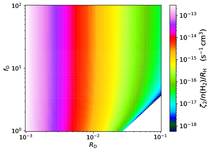
Figure 10: $\zeta_{2}$ values (divided by $R_{\mathrm{H}}\times n\rm(H_{2})$) obtained with Eq. (16) at $15\,\rm K$, as a function of $R_{\mathrm{D}}$ and $f_{\mathrm{D}}$. The bottom-right corner is missing because it violates the condition $R_{\mathrm{D}}<0.029\times f_{\mathrm{D}}$. The plot shows that the quantity $\text{$\zeta_{2}$}/(R_{\mathrm{H}}\times n\rm(H_{2}))$ increases by up to four orders of magnitude when the deuteration fraction decreases from $0.1$ to $10^{-3}$ and that the CO depletion factor plays a significant role at $R_{\mathrm{D}}$ typical for dense gas ($0.01-0.1$).

Appendix C $T_{\mathrm{ex}}$ values for $\rm DCO^{+}$ and $\rm H^{13}CO^{+}$ in LVG analysis

In Sect. 3.5 we discussed the choice of $T_{\mathrm{ex}}$ values for each transition processed with the LVG radiative transfer. Whilst those for $\rm C^{18}O$ and o$\rm H_{2}D^{+}$ are well documented in the literature, this is not the case for $\rm DCO^{+}$ and $\rm H^{13}CO^{+}$ transitions. We have corroborated the values we chose by using the online tool radex. However, in this Appendix, we investigate how a variation of the $T_{\mathrm{ex}}$ values of $\approx$20% affect the inferred $\zeta_{2}$ values. The results are shown in Fig. 11, where, in the upper panel, we analyse run 5 that uses the $\rm DCO^{+}$ and $\rm H^{13}CO^{+}$ (3-2) lines, and in the lower panel we present run 6, which instead focuses on the first rotational transitions.

In run 5, we explore a $T_{\mathrm{ex}}$ variation of $1\,$K. The resulting $\zeta_{2}$ values change by $\approx 25\%$. Note that the variation is stronger when the $T_{\mathrm{ex}}$ is lowered, due to the $T_{\mathrm{ex}}$ dependence of Eq. 2. For run 6, the values are changed by 2 K, exploring the range $8-12\,$K, which leads to a smaller variation of the inferred $\zeta_{2}$ maps (less than 10%). In all cases, the derived $\zeta_{2}$ values do not change significantly compared to the uncertainties, and the median values are still less than a factor of three from the actual input $\zeta_{2}\rm^{s}$ of the simulation.

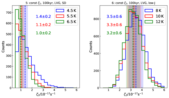
Figure 11: Histograms of the derived $\zeta_{2}$ values with the BFL20 method in run 5 (upper panel, high-J transitions) and run 6 (lower panel, low-J transitions). The different colours show different assumptions for the excitation temperature of $\rm DCO^{+}$ and $\rm H^{13}CO^{+}$ (assumed to be equal). In particular, the reference values used in the main text are shown in red (hence these data are the same presented in Fig. 1), whilst the blue/green curves show a positive/negative variation of $\approx 20$% of that value, respectively (labelled in the top-right corner of each panel). The median values and uncertainties are shown with the vertical dashed lines and shaded areas and with coloured text in each panel.

Appendix D The choice of $L$ in single-dish-like runs

To apply the analytical equations in the case of single-dish-like post-processing of the simulations, we set $L=0.3\,\rm pc$, corresponding to the size of the analysed cut-out from the original simulation box ($\rm 0.6\times 0.6\times 0.6\rm\,pc^{3}$). To support this choice and to show that this is the relevant physical quantity to take into account, we perform a further additional test. We analyse the same simulation as in the reference run n. 2, but this time we halve the size of the cut-out box before the radiative transfer. Hence, $L=0.15\,\rm pc$. The subsequent steps in terms of radiative transfer and post-processing are identical to those followed in run 2.

Our simulation consists of a box filled with molecular gas. As a consequence, most of the analysed quantities change when $L=0.15\,\rm pc$. The o$\rm H_{2}D^{+}$ column density is the only one that is not affected by this change since this molecule is highly concentrated in the densest part of the core and has a high critical density. $\rm H^{13}CO^{+}$ and $\rm C^{18}O$ suffer the largest change, and their retrieved column densities decrease by a factor of up to $2-3$. In the simulation, these two molecules are abundant everywhere, and hence cutting a smaller portion of the simulation box affects significantly their total density on the line of sight. The $\rm DCO^{+}$ column density decreases by $10-20$%. The total gas density $N(\rm H_{2})$ derived from the dust thermal emission decreases marginally ($\sim\leavevmode\nobreak\ 5$% or less). Because of these changes, $R_{\mathrm{D}}$ increases and $X\rm(CO)$ decreases, however not at the same rate. We compare the $\zeta_{2}$ maps obtained in the two tests with distinct $L$ computed with the BFL20 method in Fig. 12 (left and middle panel). The distributions of values are shown as histograms in the right panel. The maps are similar both in morphology and in the range of values. The histograms confirm these conclusions. The distributions are comparable and the median values (shown with vertical, dashed lines) are consistent with each other: ${\langle\zeta_{2}\rangle=(4.0\pm 0.7)\times 10^{-17}\,\rm s^{-1}}$ (${L=0.3\,\rm pc}$) and ${\langle\zeta_{2}\rangle=(3.7\pm 0.8)\times 10^{-17}\,\rm s^{-1}}$ (${L=0.15\,\rm pc}$). If we used the old value $L=0.3\rm\,pc$ in the new test with a smaller box, the blue histogram would shift to the left (towards lower values) by a factor of two.

This test suggests that using the size of the cut-out box to estimate $L$ in these runs is an appropriate choice. We stress again that this is a consequence of the particular simulation we are investigating, which represents a rather dense medium where most of the molecules of interest are abundant in the entire box. This is not the case for isolated cores such as the ones tested in Sect. 4.3 of the manuscript, for which the prescription based on the $N(\rm H_{2})$ isocontour is appropriate.

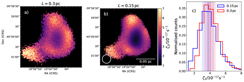
Figure 12: Comparison of the resulting $\zeta_{2}$ maps (in units of $10^{-17}\,\rm s^{-1}$) on the two runs with distinct box sizes $L$ but otherwise identical, using the BFL20 method. Panel a) shows the run with $L=0.3\,\rm pc$ (i.e. the reference run 2), and panel b) shows the results with $L=0.15\rm\,pc$. The colorbar is kept fixed to ease the comparison. The histogram distributions are compared in panel c), labelled in the top-right corner. The median values (median uncertainties) are shown with the vertical dashed lines (shaded areas).