Manipulation Test for Multidimensional RDD

The causal inference model proposed by lee2008randomized for the regression discontinuity design (RDD) relies on assumptions that imply the continuity of the density of the assignment (running) variable. The test for this implication is commonly referred to as the manipulation test and is regularly reported in applied research to strengthen the design’s validity. The multidimensional RDD (MRDD) extends the RDD to contexts where treatment assignment depends on several running variables. This paper introduces a manipulation test for the MRDD. First, it develops a theoretical model for causal inference with the MRDD, used to derive a testable implication on the conditional marginal densities of the running variables. Then, it constructs the test for the implication based on a quadratic form of a vector of statistics separately computed for each marginal density. Finally, the proposed test is compared with alternative procedures commonly employed in applied research.

Keywords: Regression Discontinuity Design, Manipulation Test, Multidimensional RDD
JEL classification codes: C12, C14

1 Introduction

Regression Discontinuity Design (RDD) is widely used in policy evaluation and causal inference analysis to establish credible causal relationships under mild assumptions. RDD requires that units are assigned to a treatment based on some observable characteristic, the running variable: the probability of being treated must discontinuously change when the value of the running variable exceeds a certain threshold, called the cutoff. The fact that policies are often designed in this way (scholarship for students with GPA exceeding a threshold, welfare benefits for households with a certain income, etc.) explains RDD popularity.

To identify the average treatment effect (ATE) at the cutoff, the model for causal inference with the RDD proposed by lee2008randomized requires assumptions on unobservable potential outcomes. Albeit these assumptions are not directly testable, the model entails two implications on observable quantities, which can be tested. The first implication requires continuity at the cutoff for the probability density function of the running variable. The second imposes continuity at the cutoff for the conditional (on the running variable) expectation of additional observable characteristics measured before the treatment. Tests of these implications provide evidence of the RDD validity and are commonly reported in empirical applications, as highlighted by the survey in canay2018approximate. The one for the continuity of the density of the running variable is known as the manipulation test since it checks that units do not manipulate their scores to get assigned to treatment. Several manipulation tests have been proposed in the literature, from the seminal one by mccrary2008manipulation to more recent approaches by cattaneo2020simple and bugni2021testing.

This paper introduces a manipulation test for the multidimensional RDD (MRDD), valid for both cases of perfect (sharp MRDD) and imperfect (fuzzy MRDD) compliance. MRDD is a model where the treatment assignment depends on multiple running variables. I consider the version of MRDD where the probability of receiving the treatment changes discontinuously when all the running variables exceed their cutoffs, and the cutoff of each running variable is fixed. Compared to the single-dimensional RDD, the main novelty is that the cutoff is not a point in a single-dimensional space but a set of infinite points in the multidimensional space of the running variables. Consider, for example, a scholarship for students who score above certain thresholds in language and mathematics tests, as illustrated in figure 1. The MRDD allows the researcher to identify and estimate the average effect of the scholarship on students with scores at the boundary. In this case, the cutoff is the solid purple boundary in the bi-dimensional space of language and math scores.

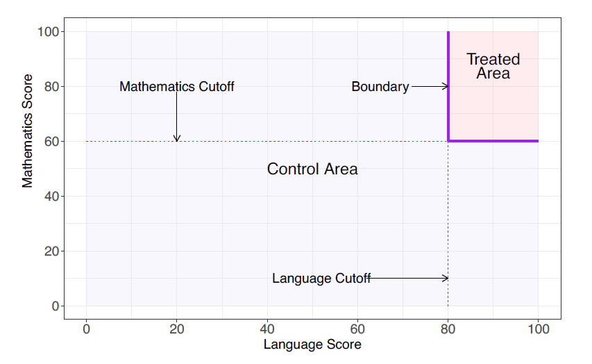
Figure 1: MRDD running variables and thresholds. Source: cattaneo2019practicale

The main contributions of this paper are the following: first, I extend the lee2008randomized’s model to the multidimensional setting and derive a testable implication on the conditional marginal densities of the running variables. Then, I construct a manipulation test for the implication, which helps corroborate the MRDD’s credibility. Intuitively, the test procedure first divides the space of running variables into subspaces where only one variable determines the treatment assignment. In each subspace, the model implication requires the marginal density of the now single-running variable to be continuous at its single-dimensional threshold. I then obtain a set of conditions on the continuity of conditional marginal densities of all running variables and propose a multidimensional manipulation test based on a quadratic form of the test statistics considered by cattaneo2020simple for the single-dimensional case, computed for each implication. Asymptotically, these statistics converge to a multivariate normal distribution, and my test statistic to a chi-square with as many degrees of freedom as the number of running variables.

I am not the first to study MRDD from a theoretical perspective. Identification and estimation in the MRDD setting, and how they differ from the single-dimensional RDD, have been investigated by imbens2009regression and papay2011extending, respectively; other results are also discussed in wong2013analyzing, and imbens2019optimized. So far, to my knowledge, there is no research explicitly dealing with extending the framework proposed by lee2008randomized and discussing manipulation tests in the MRDD context. Interestingly, though, manipulation tests are run by several applied papers employing MRDD (see the survey in table 1): they appeal to disparate approaches, with different null hypotheses, assumptions, and test statistics. None of these approaches justifies the implemented procedures, while my test is supported by a model and backed by statistical theory. Local asymptotic analysis and Monte Carlo simulations confirm my test’s advantages in terms of size control and power in realistic settings.

Three main strands of literature resort to MRDD as a tool for causal inference. First, it is exploited to evaluate policies that assign a treatment when more than one condition on observable continuous quantities is met. Examples can be found in several fields, mainly in education (matsudaira2008mandatory; clark2014signaling; cohodes2014merit; elacqua2016short; evans2017smart; smith2017giving; londono2020upstream) but also in corporate finance (becht2016does), political economy (hinnerich2014democracy; frey2019cash), development (salti2022impact), industrial organization (snider2015barriers), and public economics (egger2015impact). In these cases, MRDD provides reliable results on treatment effects from a clean identification strategy.

A second application is the geographic or spatial RDD to study the effect of treatments only assigned to specific areas. Running variables are latitude and longitude, and the boundary at which the ATE is computed coincides with actual (or historical) national, regional, or municipal borders. keele2015geographic discuss how this setting relates to MRDD in detail. Note, however, that I am considering a model where the treatment is assigned when each running variable exceeds its cutoff: as such, my results do not directly apply to the spatial RDD, and if my test works in this setting, it is a case-specific issue.

Third, recently there has been an increasing interest in MRDD in a theory literature at the intersection of market design and machine learning (abdulkadiroglu2022breaking; narita2021algorithm). When algorithms determine a treatment assignment, they may consider multiple thresholds and running variables in a setting that mimics an MRDD. This literature is primarily theoretical, but it will likely encourage new empirical research, potentially relying on my proposed manipulation test.

The rest of the paper is organized as follows. Section 2 develops the theoretical model for MRDD and derives the testable implication. Section 3 provides a manipulation test for the implication. Section 4 compares the manipulation test with alternative approaches used in the literature. Section 5 reports Monte Carlo simulations. Section 6 applies the manipulation test to frey2019cash. Section 7 concludes.

2 Model

2.1 Model for MRDD

I extend the model proposed by lee2008randomized to the multidimensional setting, allowing the number of running variables $d$ to be larger than one and incorporating the identification results provided by imbens2009regression. The extension is needed to derive the testable implication for the manipulation test.

Let $W$ be a random variable with support $\mathcal{W}$ and density $g(w)$. $W$ indicates the type of agents, unobservable to the researcher, and can be discrete or continuous, with finite or infinite support.

Let $Z\in\mathbb{R}^{d}$ be a random vector of $d$ observable continuous running variables with joint cumulative distribution function $F(z)$ and marginal CDFs $F_{j}(z_{j})$.

The treatment status $D$ depends on $Z$: I consider a sharp design where the treatment status depends deterministically on $Z$. The model can also be extended to a fuzzy design, where the probability of being treated changes discontinuously at the threshold. Units are treated ($D=1$) when all components of $Z$ are above a certain threshold:

$$D=D(Z)=\mathbf{1}\{Z\geq c\}=\mathbf{1}\{Z_{1}\geq c_{1}\}\mathbf{1}\{Z_{2}\geq c_{2}\}\dots\mathbf{1}\{Z_{d}\geq c_{d}\}$$ (1)

and $D=0$ otherwise. Without loss of generality, consider a rescaling of $Z$ such that $c_{j}=0$, for all $j$: units are treated when, for all $j$, $Z_{j}\geq 0$.

Let $\mathcal{T}$ be the set of values of $Z$ for which $D(Z)=1$, and indicate with $\bar{\mathcal{T}^{C}}$ the closure of the complement of $\mathcal{T}$. Define the boundary $\mathcal{B}=\mathcal{T}\cap\bar{\mathcal{T}^{C}}$, and note that, by definition, in a neighborhood of any point $b\in\mathcal{B}$ there are both treated and untreated units.

Let $F(z|w):\mathbb{R}^{d}\times\mathcal{W}\rightarrow[0,1]$ be the cdf of $Z$ conditional on $W$.

Assumption 1.

(Continuity of density) For all $w\in\mathcal{W}$, for all $b\in\mathcal{B}$, $F(z|w)$ is continuously differentiable in $z$ at $b$. Furthermore, the conditional density $f(z|w)$ is bounded away from zero at $b$.

Assumption 1 is asking the conditional density $f(z|w)$ of the running variables $Z$ to be continuous and non-zero at $b\in\mathcal{B}$, for all $w$. The testable implication for the manipulation test is derived from this assumption. It does not entirely exclude influence over the score vector $Z$: some manipulation is allowed, as long as it is not deterministic, as discussed in section 2.3.

The researcher observes an iid sample from the joint distribution of $\{Z,D,Y\}$, where the observed outcome $Y$ is defined as $Y=(1-D)Y_{0}+DY_{1}$. Potential outcomes $Y_{0}=y_{0}(W,Z)$ and $Y_{1}=y_{1}(W,Z)$ are random functions of $W$ and $Z$. For each value of agent type $W$ and running variable $Z$, $y_{0}(w,z)$ and $y_{1}(w,z)$ are random variables, and their distributions satisfy the following assumption.

Assumption 2.

(Continuity of expectation of potential outcomes) For all $w\in\mathcal{W}$, for all $b\in\mathcal{B}$, expected potential outcomes $\mathbb{E}[y_{0}(w,z)]$ and $\mathbb{E}[y_{1}(w,z)]$ are continuous in $z$ at $b$.

Intuitively, the MRDD compares treated and untreated units close to the boundary. Assumption 2 guarantees that the local information from the observable quantities on one side of the boundary is informative about the unobservable quantities on the other side.

The parameters of interest are $\tau(b)$ and $\tau$. $\tau(b)$ is the Conditional Average Treatment Effect (CATE):

$$\tau(b)=\mathbb{E}[Y_{1}-Y_{0}|Z=b],\quad b\in\mathcal{B}$$

and $\tau$ is the Integrated Conditional Average Treatment Effect (ICATE):

$$\tau=\mathbb{E}[Y_{1}-Y_{0}|Z\in\mathcal{B}].$$

The CATE is a function that maps every point on the boundary to an average treatment effect, while the ICATE aggregates these effects into a single parameter.

Theorem 1 is the main result for identification in the multidimensional setting.

Theorem 1.

(Identification of $\tau(b)$ and $\tau$) Under Assumptions 1 and 2, $\tau(b)$ and $\tau$ are identified.

The result in Theorem 1 can be seen as a generalization of lee2008randomized that does not require $\mathcal{B}$ to be a singleton and specifies new parameters of interest, suitable for the MRDD (in the single-dimensional case, $\tau(b)$ and $\tau$ coincide).

2.2 Testable implication

Assumption 1 involves the unobservable types $w$, and cannot be directly tested. Nonetheless, it has a testable implication on the observable distribution of $Z$, derived in the following proposition.

Proposition 1.

(Testable implication) Assumption 1 implies the following condition on observable quantities:

$$f_{Z_{j}|Z_{-j}}(z_{j}|z_{-j}\geq 0)\text{ continuous at }z_{j}=0,\forall j.$$ (2)

Proposition 1 derives the null hypothesis of the manipulation test for the MRDD developed in this paper. It requires the marginal density of each running variable to be continuous close to the boundary. Compared with other conditions that can be derived from assumption 1, the implication has two suitable advantages: it concerns continuity in a finite set of points and maintains a straightforward interpretation in terms of restrictions on agents behavior, excluding manipulation for any of the $d$ running variables.

The implication is not sharp, since it is possible for $f_{Z_{j}|Z_{-j}}(z_{j}|z_{-j}\geq 0)$ to be continuous even if $f(z|w)$ is not. This issue does not depend on $d$ being larger than 1, and it analogously arises in the single-dimensional case: see lee2008randomized for further discussion.

2.3 Example

The example depicted in figure 1 is helpful to gain some intuition of the model. A scholarship is assigned to students who score above certain thresholds in both math and language tests, and a researcher is interested in the average effect of the scholarship on, for example, the probability of college admission. The scholarship is not randomly assigned, and comparing the average college attendance rates between the treated and untreated groups can be misleading. Even with no effects of the scholarship, for example, we may expect higher college attendance for students who did well on the math and language tests, because of unobservable characteristics, such as effort, correlated with the scores. Consider, however, a combination of math and language scores on the solid purple boundary in the picture. All students are similar in a neighborhood of those scores, except for their treatment status. To compute the CATE $\tau(b)$ of the scholarship for students with that specific combination of math and language scores, the researcher may compare locally treated and untreated units close to that score. The procedure can be applied to every combination of math and language scores at the boundary, and the estimated effects, dependent on the considered point of the boundary, can be aggregated in a unique average treatment effect, the ICATE $\tau$.

I mentioned that assumption 1 does not entirely exclude influence over the score vector $Z$: some manipulation is allowed, as long as it is not deterministic. For example, assumption 1 is satisfied if, whatever the type $w$, $Z$ can be decomposed as $Z=V+\epsilon$, with $V$ and $\epsilon\in\mathbb{R}^{d}$, $V$ a deterministic part, perfectly controllable by agents, and dependent on the type $w$, and $\epsilon$ a random component with continuous density. In the scholarship context, imagine two student types: $w_{1}$ and $w_{2}$. Students type $w_{1}$ are not interested in the scholarship, which does not influence their behavior. Assumption 1 is satisfied for them. Students type $w_{2}$, instead, want to secure the scholarship but also know that their score in language or math is below the threshold. They decide to study harder to improve their score and win the scholarship. Since studying is costly and they want to minimize their effort, they choose to improve their score to a level $V$ just at the boundary. The density of $V$ is not continuous at $\mathcal{B}$. However, the test score may have a random component $\epsilon$ that students cannot perfectly control: it may be their focus on the test day. Despite all students type $w_{2}$ having the same $V$, not all get the same score $Z$, and as long as $\epsilon$ has continuous density, $f(z|w_{2})$ is continuous at the boundary $\mathcal{B}$. Even in the case of stochastic manipulation, hence, assumption 1 is satisfied.

3 Manipulation Test

To test the implication in Proposition 1, consider the manipulation test $\phi(\hat{t},\alpha)$, defined as follows:

$$\phi(\hat{t},\alpha)=\begin{cases}1,&\text{if $\hat{t}>c(\alpha)$}\\ 0,&\text{if $\hat{t}\leq c(\alpha)$}\end{cases}$$ (3)

where $\hat{t}$ is the test statistic, $\alpha$ the significance level, and $c(\alpha)$ the critical value. Whenever $\phi(\hat{t},\alpha)$ equals 1, the null hypothesis specified in equation 23 is rejected.

Constructing the test statistic $\hat{t}$ involves two steps. First, for each running variable $j$, compute the statistic $\hat{\theta}_{j}$ along with its variance $\hat{\sigma}^{2}_{j}$. The expression for $\hat{\theta}_{j}$ is given by:

$$\hat{\theta}_{j}=\hat{f}^{+}_{Z_{j}|Z_{-j}}(0|z_{-j}\geq 0)-\hat{f}^{-}_{Z_{j}|Z_{-j}}(0|z_{-j}\geq 0)$$ (4)

where $\hat{f}^{+}_{Z_{j}|Z_{-j}}$ and $\hat{f}^{-}_{Z_{j}|Z_{-j}}$ are estimators of the conditional marginal density of $Z_{j}$ (the formula for $\hat{f}^{+}_{Z_{j}|Z_{-j}}$ and $\hat{f}^{-}_{Z_{j}|Z_{-j}}$ will be provided in section 3.1). It is worth noting that $\hat{\theta}_{j}$ resembles the test statistic proposed by cattaneo2020simple for testing the continuity of the density in the single-dimensional RDD. The difference is that here, the test is on the continuity of a conditional marginal density, which necessitates some adaptations for the statistic and the formal proofs.

Next, construct the test statistic $\hat{t}$ based on the vector $\hat{\theta}=(\hat{\theta}_{1},\dots,\hat{\theta}_{d})$ and the diagonal matrix $\hat{\Sigma}=\text{diag}(\hat{\sigma}^{2}_{1},\dots,\hat{\sigma}^{2}_{d})$. The test statistic $\hat{t}$ is the quadratic form given by:

$$\hat{t}=\hat{\theta}^{\prime}\hat{\Sigma}^{-1}\hat{\theta}.$$

The vector $\hat{\theta}$ converges in distribution to a multivariate normal distribution, and the test statistic $\hat{t}$ converges to a $\chi^{2}$ with $d$ degrees of freedom. Consequently, the critical value $c(\alpha)$ corresponds to the $1-\alpha$ quantile of a $\chi^{2}$ distribution with $d$ degrees of freedom. If the test statistic exceeds this critical value, the manipulation test rejects the null hypothesis.

3.1 Assumptions

The following assumptions are needed to establish the asymptotic validity of the test $\phi(\hat{t},\alpha)$.

Assumption 3.

(Smothness) $\{z_{i}\}_{i\in\{1,\dots,n\}}$ is an iid random sample of $Z$ with cumulative distribution function $F$. In neighborhoods of points on the boundary $\mathcal{B}$, $F$ is at least four times continuously differentiable.

The assumption that $F$ has at least four continuous derivatives allows to employ a consistent method to select the bandwidth for the estimators $\hat{f}^{+}_{Z_{j}|Z_{-j}}$ and $\hat{f}^{-}_{Z_{j}|Z_{-j}}$. The manipulation test of mccrary2008manipulation requires the same condition for the single-dimensional case.

Assumption 4.

(Kernel) The kernel function $K(.)$ is nonnegative, symmetric, continuous, and integrates to one: $\int K(u)du=1$. It has support $[-1,1]$.

The bounded support for the kernel helps save the notation but is not crucial for the results. To further simplify the notation, define

$$f_{j}(z_{j})=f_{Z_{j}|Z_{-j}}(z_{j}|z_{-j}\geq 0).$$

Consider the local polynomial estimator $\hat{f}_{j,p}(z_{j})$:

$$\hat{f}_{j,p}(z_{j})=e_{1}^{\prime}\hat{\beta}(z_{j})$$

$$\hat{\beta}(z_{j})=\text{argmin}_{b\in\mathbb{R}^{p+1}}\sum_{i=1}^{n}\left[\tilde{F_{j}}(z_{j}|z_{-j}\geq 0)-r_{p}(z_{ji}-z_{j})^{\prime}b\right]^{2}K\left(\frac{z_{ji}-z_{j}}{h_{j}}\right)\mathbf{1}\{z_{-j}\geq 0\}$$

where $e_{1}^{\prime}\in\mathbb{R}^{p+1}$ such that $e_{1}^{\prime}=(0,1,0,\dots,0)$; $n_{j}=\sum_{i=1}^{n}\mathbf{1}\{z_{-j}\geq 0\}$ is the number of observations actually considered for the test; $\tilde{F_{j}}(z_{j}|z_{-j}\geq 0)=\frac{1}{n_{j}}\sum_{i}\mathbf{1}\{z_{ji}\leq z_{j}\}\mathbf{1}\{z_{-ji}\geq 0\}$ is the empirical distribution function for the marginal conditional distribution $F(z_{j}|z_{-j}\geq 0)$; $r_{p}(u)=(1,u,u^{2},\dots,u^{p})$ is a one-dimensional polynomial expansion; and $h_{j}$ is a bandwidth, which will be better specify later.

With a sample of size $n$, the estimator $\hat{f}_{j,p}(z_{j})$ considers only the $n_{j}$ observations with $z_{-j}\geq 0$. Let $\pi_{j}=Pr(z_{-j}\geq 0)$: by the strong law of large number, as $n\to\infty$, $\frac{n_{j}}{n}\rightarrow^{a.s.}\pi_{j}$. Since $\pi_{j}\in(0,1)$, with probability 1, as $n\to\infty$, $n_{j}\to\infty$. Analogously, define $\pi_{j+}=Pr(z_{j}\geq 0|z_{-j}\geq 0)$, and $\pi_{j-}=Pr(z_{j}\leq 0|z_{-j}\geq 0)$.

The local polynomial approach for estimating derivatives of the cumulative distribution function was introduced by jones1993simple and fan2018local. This method is particularly well-suited for the manipulation test as it achieves the optimal rate of convergence both in interior points and at the boundaries, and is boundary adaptive. No adjustment is required when computing estimates for points near the boundary if the object of interest is the $\nu$-th derivative and $p-\nu$ is odd. In the case of my manipulation test, where $\nu=1$, I will use an estimator with $p=2$ to take advantage of its boundary adaptiveness.

3.2 Manipulation Test

To establish the validity of the test $\phi(\hat{t},\alpha)$, it is necessary to derive some intermediate results. The first result regards the asymptotic properties of the density estimator $\hat{f}_{j,p}(z_{j})$. Formulas for bias $B(x)$, variance $V(x)$, and consistent variance estimator $\hat{V}(x)$ are reported in Appendix A.

Proposition 2.

(Asymptotic distribution of $\hat{f}_{j,p}(z_{j})$) Under Assumptions 1, 3 and 4, with $p=2$, $nh_{j}^{2}\rightarrow\infty$ and $nh_{j}^{2p+1}=O(1)$, $\hat{f}_{j,p}(z_{j})$ is a consistent estimator for $f_{j}(z_{j})$. Furthermore,

$$\sqrt{n_{j}h_{j}}(\hat{f}_{j,p}(z_{j})-f_{j}(z_{j})-h_{j}^{p}B(z_{j}))\rightarrow^{d}\mathcal{N}(0,V(z_{j}))$$ (5)

where $B(z_{j})$ is the asymptotic bias.

When $nh_{j}^{2p+1}=O(1)$, the bandwidth $h_{j}$ has the MSE-optimal rate and can be computed by cross-validation.

The presence of asymptotic bias $B(z_{j})$ is standard in nonparametric settings and must be considered to ensure valid hypothesis testing. In this paper, I adopt the robust bias correction method proposed by calonico2018effect. Alternative approaches include the critical values correction method suggested by armstrong2020simple.

Bias-corrected inference for the density estimator $\hat{f}_{j,p}(z_{j})$ can be obtained by considering the estimator $\hat{f}_{j,q}(z_{j})$ with $q=p+1$, computed with the bandwidth $h_{j,p}$, the MSE-optimal bandwidth for $\hat{f}_{j,p}(z_{j})$ (see calonico2022coverage and cattaneo2019lpdensity for an extensive discussion on the procedure). Going forward, I will consider estimator $\hat{f}_{j,p}(z_{j})$ for point estimates, and estimator $\hat{f}_{j,q}(z_{j})$ with bandwidth $h_{j,p}$ to construct bias-corrected confidence intervals for $\hat{f}_{j,p}(z_{j})$.

Let $n_{j+}=\sum_{i=1}^{n}\mathbf{1}\{z_{j}\geq 0\}\mathbf{1}\{z_{-j}\geq 0\}$ and $n_{j-}=\sum_{i=1}^{n}\mathbf{1}\{z_{j}<0\}\mathbf{1}\{z_{-j}\geq 0\}$, and indicate with $\frac{n_{j+}}{n_{j}}\hat{f}_{j+,p}(z_{j})$ and $\frac{n_{j-}}{n_{j}}\hat{f}_{j-,p}(z_{j})$ the estimators of conditional density $f_{j}(z_{j})=f_{Z_{j}|Z_{-j}}(z_{j}|z_{-j}\geq 0)$ computed considering only observations in $\{z:z\geq 0\}$ and $\{z:z_{j}<0,z_{-j}\geq 0\}$, respectively.

Consider $\theta_{j}=\lim_{z_{j}\rightarrow 0^{+}}f_{j}(z_{j})-\lim_{z_{j}\rightarrow 0^{-}}f_{j}(z_{j})$, and note that, if the condition in Proposition 1 is true, $\theta_{j}=0$ for all $j$. Define the statistic $\hat{\theta}_{j,p}$:

$$\hat{\theta}_{j,p}=\frac{n_{j+}}{n_{j}}\hat{f}_{j+,p}(0)-\frac{n_{j-}}{n_{j}}\hat{f}_{j-,p}(0).$$ (6)

The following result derives the asymptotic distribution of the statistic.

Proposition 3.

(Asymptotic distribution of $\hat{\theta}_{j,q}$) Under Assumptions 1, 3 and 4 holding separately for $\{Z:Z\geq 0\}$ and $\{Z:Z_{-j}\geq 0,Z_{j}<0\}$, with $p=2$, $q=p+1$, $n\min\{h_{j-},h_{j+}\}\rightarrow\infty$, and $n\max\{h_{j-}^{1+2q},h_{j+}^{1+2q}\}\rightarrow 0$, when the implication $\theta_{j}=0$ is true:

$$\frac{1}{\sigma_{j}}\hat{\theta}_{j,q}\rightarrow^{d}\mathcal{N}\left(0,1\right)$$ (7)

where

$$\sigma_{j}^{2}=\frac{\pi_{j+}}{h_{j+}\pi_{j}n}V_{j+}(0)+\frac{\pi_{j-}}{h_{j-}\pi_{j}n}V_{j-}(0).$$ (8)

A consistent estimator $\hat{\sigma}_{j}^{2}$ for $\sigma_{j}^{2}$ can be obtained by

$$\hat{\sigma}_{j}^{2}=\frac{n_{j+}}{h_{j+}n_{j}^{2}}\hat{V}_{j+,q}(0)+\frac{n_{j-}}{h_{j-}n_{j}^{2}}\hat{V}_{j-,q}(0).$$ (9)

Proposition 3 is valid for any $j$. I am interested in the asymptotic distribution of the vector $\hat{\theta}=(\hat{\theta}_{1},\hat{\theta}_{2},\dots,\hat{\theta}_{d})$, whose distribution under the null hypothesis of continuity of $f_{Z_{j}|Z_{-j}}(z_{j}|z_{-j}\geq 0)$ is derived in the next theorem.

Theorem 2.

(Asymptotic distribution of $\hat{\theta}$) Under Assumptions 1, 3 and 4 holding separately for $\{Z:Z\geq 0\}$ and $\{Z:Z_{-j}\geq 0,Z_{j}<0\}$ for all $j$, with $p=2$, $q=p+1$, $n\min\{h_{j-},h_{j+}\}\rightarrow\infty$ and $n\max\{h_{j-}^{1+2q},h_{j+}^{1+2q}\}\rightarrow 0$ for all $j$, when $\theta=0$,

$$\hat{\Sigma}^{-\frac{1}{2}}\hat{\theta}\rightarrow^{d}\mathcal{N}(0,I).$$

where $\hat{\Sigma}_{jj}=\hat{\sigma}^{2}_{j}$ as defined in Proposition 3, and $\hat{\Sigma}_{ji}=0$ for all $i\neq j$.

Theorem 2 shows how, even if the number of observations simultaneously considered by estimators $\theta_{j}$ and $\theta_{i}$ goes to infinite, they are asymptotically independent.

Corollary 1.

(Asymptotic distribution of $g(\hat{\Sigma}^{-\frac{1}{2}}\hat{\theta})$) Let $g$ be a continuous function, and $X\in\mathbb{R}^{d}$ a random vector with distribution $\mathcal{N}(0,I)$. Theorem 2 and continuous mapping theorem imply that the statistic $g(\hat{\Sigma}^{-\frac{1}{2}}\hat{\theta})$ converges in distribution to $g(X)$.

Corollary 1 holds for any continuous function $g$. As test statistic, I consider the quadratic form $\hat{t}=g(\hat{\Sigma}^{-\frac{1}{2}}\hat{\theta})=\hat{\theta}^{\prime}\hat{\Sigma}^{-1}\hat{\theta}$. While it is not the only function suitable for constructing a consistent test (an alternative using the max-statistic $\hat{t}_{m}=\max\left(|\frac{\hat{\theta}_{1}}{\hat{\sigma}_{1}}|,\dots,|\frac{\hat{\theta}_{d}}{\hat{\sigma}_{d}}|\right)$ is discussed in Appendix B), the quadratic form proves particularly effective in detecting manipulation diffused across multiple running variables. These are behaviors of primary interest: in contexts where the treatment’s benefits lead agents to manipulate their running variables for eligibility, the manipulation is likely to be widespread.

The critical value $c(\alpha)$ is the $1-\alpha$ quantile of a $\chi^{2}$ distribution with $d$ degrees of freedom. Recall that the manipulation test for the MRDD $\phi(\hat{t},\alpha)$ is defined as:

$$\phi(\hat{t},\alpha)=\begin{cases}1,&\text{if $\hat{t}>c(\alpha)$}\\ 0,&\text{if $\hat{t}\leq c(\alpha)$}\end{cases}$$ (10)

with the null hypothesis rejected when $\phi(\hat{t},\alpha)=1$. When the null hypothesis in Proposition 1 is true, the test has an asymptotic rejection probability of $\alpha$. When the null hypothesis is false, the test asymptotically rejects with probability 1. The following corollary formalizes this result.

Corollary 2.

(Manipulation test) Let $H_{0}$ be the null hypothesis reported in equation 23. Under the assumptions of Theorem 2, when $H_{0}$ is true:

$$\lim_{n\rightarrow\infty}P(\phi(\hat{t},\alpha)=1)=\alpha.$$ (11)

When $H_{0}$ is false:

$$\lim_{n\rightarrow\infty}P(\phi(\hat{t},\alpha)=1)=1.$$ (12)

4 Alternative approaches

It is common for applied papers utilizing the regression discontinuity design to include manipulation tests for their running variables, as highlighted by the survey by canay2018approximate. Although there is a lack of a theoretical foundation for the test in the multidimensional case, table 1 attests the prevalence of manipulation tests in papers employing the MRDD. These papers typically employ two different approaches: computing multiple tests, one for each running variable separately (Separate Tests, ST); or aggregating the running variables considering the distance of each observation from the boundary, and then running the manipulation test for the distance as the single running variable (Distance as running variable Test, DT). The ST approach does not control the size for the null hypothesis in Proposition 1, while the DT is not consistent against certain alternatives, and is not robust to change in the units of measure. In the following sections, I compare these approaches with the proposed manipulation test (MT). I highlight their limitations and show how they can be adapted to properly test the null hypothesis in Proposition 1.

Table 1: Published papers using MRDD. Most studies utilize either separate tests (ST), where each running variable’s density continuity is tested individually, or distance as running variable tests (DT), which consider the distance of observations from the boundary as the unique running variable.

Authors (Year)	Manipulation Test	ST	DT
frey2019cash	$\times$
matsudaira2008mandatory	✓	✓
hinnerich2014democracy	✓	✓
elacqua2016short	✓	✓
egger2015impact	✓	✓
evans2017smart	✓	✓
smith2017giving	✓	✓
londono2020upstream	✓	✓
clark2014signaling	✓		✓
cohodes2014merit	✓		✓
becht2016does	✓		✓

4.1 Separate Tests (ST)

The separate tests procedure in the context of MRDD treats each running variable separately and applies existing manipulation tests designed for single-dimensional RDD (mccrary2008manipulation; cattaneo2020simple; bugni2021testing). In some cases (egger2015impact; evans2017smart; londono2020upstream), the test is conducted on the conditional marginal densities by considering only the units that meet the threshold for the other running variables. Either way, without accounting for multiple hypotheses testing, the ST is invalid, as it does not control the size for the null in equation 23.

4.2 Multiple hypotheses test with Bonferroni correction (BCT)

A straightforward fix for the ST is to account for multiple hypotheses testing using Bonferroni correction (BCT). In case the test by cattaneo2020simple is employed, the resulting procedure partly overlaps with the test I proposed. To test the implication in Proposition 1 at level $\alpha$, statistics $\hat{\theta}_{j}$ defined in equation (6) are used to conduct separate tests for each running variable, with the critical values adjusted for multiple testing (for a review on multiple hypotheses testing, see chapter 9 in lehmann2022testing). The null hypothesis of running variable $j$ continuity is tested at significance level $\frac{\alpha}{d}$, where $d$ is the number of running variables. The implication in Proposition 1 is rejected if the continuity of any of the running variables is rejected. The correction for the number of hypotheses ensures correct coverage, meaning that the asymptotic family-wise error rate, which is the probability of rejecting one or more true null hypotheses (and hence the probability of rejecting the implication in Proposition 1 when it is true), is not greater than $\alpha$. In this context, alternative multiple hypotheses corrections (e.g., stepwise methods or Holm correction) would coincide with the BCT, as rejecting continuity for the density of just one running variable is equivalent to rejecting the implication in Proposition 1.

MT and BCT rely on the same vector of statistics $\hat{\theta}$. Local power analysis can be used to compare the power of the two tests against local alternative hypotheses, letting the discontinuity of the density at the threshold get smaller as the sample size increases. I consider two frameworks. In the first framework, all the running variables are discontinuous, and the discontinuity is equal to $k/\sqrt{nh}$, such that, asymptotically, $\hat{\theta}_{j}\rightarrow^{d}\mathcal{N}(k,1)$ for all $j$. In the second framework, only running variable $j=1$ is discontinuous, such that $\hat{\theta}_{1}\rightarrow^{d}\mathcal{N}(k,1)$ and $\hat{\theta}_{j}\rightarrow^{d}\mathcal{N}(0,1)$ for $j\neq 1$. The first framework mimics a setting where all the running variables are manipulated to get the treatment: if treatment is desirable (or undesirable), I may expect all the agents close to the treatment region to manipulate their running variables to get in (or out) the region. In the scholarship example, students want to manipulate both language and math scores to get the scholarship. The second framework depicts a situation where manipulation only occurs for one running variable: this may happen because running variables are different, and some could be impossible to manipulate. Suppose, for example, that mock exams for the language test are unavailable: students cannot manipulate the language score, while they can manipulate the math one.

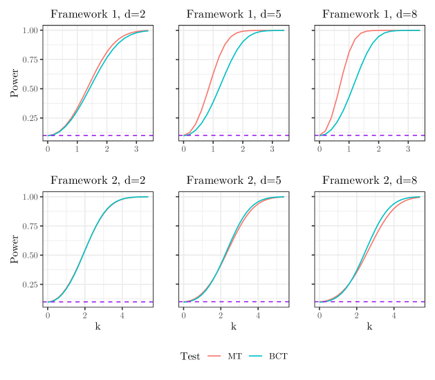
Figure 2: Local asymptotic power curves for the manipulation test proposed in this paper (MT, in red) and the multiple hypotheses test with Bonferroni correction (BCT, in blue). Plots consider different frameworks and different numbers $d$ of running variables. The significance level $\alpha=0.1$ is represented by the dotted horizontal purple line. In Framework 1, all the running variables are discontinuous, and the discontinuity is equal to $k/\sqrt{nh}$, such that $\hat{\theta}_{j}\rightarrow^{d}\mathcal{N}(k,1)$ for all $j$. In Framework 2, only running variable $j=1$ is discontinuous, such that $\hat{\theta}_{1}\rightarrow^{d}\mathcal{N}(k,1)$ and $\hat{\theta}_{j}\rightarrow^{d}\mathcal{N}(0,1)$ for $j\neq 1$.

Figure 2 reports power curves for MT (in red) and BCT (in blue) in the two frameworks, considering different numbers of running variables $d\in\{2,5,8\}$. In the first framework, where all running variables exhibit discontinuity, MT outperforms BCT in terms of power. This is because MT combines information from all the running variables and effectively detects manipulation when it is widespread across them. On the other hand, BCT considers each running variable separately, which results in lower power in case of widespread manipulation. Distance between the curves increases with the number of running variables $d$.

In the second framework, results are subtler. For small values of the discontinuity parameter ($k$), MT remains more powerful. However, as $k$ increases, the order is reversed, and BCT becomes more powerful. Combining information may dilute the signal from the discontinuous running variable and is no longer a strictly better choice. Monte Carlo simulation confirms that MT and BCT have a comparable finite sample performance. In these settings, where manipulation is not widespread and concerns only one running variable, the max-statistic $\hat{t}_{m}=\max\left(|\frac{\hat{\theta}_{1}}{\hat{\sigma}_{1}}|,\dots,|\frac{\hat{\theta}_{d}}{\hat{\sigma}_{d}}|\right)$ may guarantee a manipulation test with better power: this procedure is investigated in appendix B.

4.3 Distance as running variable test (DT)

The second approach for manipulation tests in the multidimensional setting employed in applied research involves a different type of dimension reduction: the multidimensional regression discontinuity design is reduced to a single-dimensional design, with the scalar distance between the vector of running variables and the boundary $\mathcal{B}$ as the only running variable. The distance is used to estimate the conditional average treatment effect, similar to the classical RDD, and to conduct a manipulation test using one of the available tests (mccrary2008manipulation; cattaneo2020simple; bugni2021testing). This approach appears simple since it directly relates to the single-dimensional RDD case. Nonetheless, it comes with some caveats that need to be considered.

First, the choice of distance metric and measurement units can significantly impact the test results. Different distance metrics used to measure the distance between the running variables and the boundary lead to different test statistics and test outcomes, as well as different units of measurement for the running variables. To address this second issue, one possible solution is to standardize the running variables to have unit variance before conducting the manipulation test, even if, as far as I know, no clear explanation justifies this practice.

A second flaw of the DT is that it is inconsistent against certain fixed alternatives of the null hypothesis in equation (23). For instance, if there are opposite discontinuities in the marginal distributions of different running variables, and these discontinuities balance each other out, the asymptotic probability that the DT will reject the false null hypothesis in equation (23) is equal to $\alpha$, rather than one. A design where the DT test is inconsistent is studied in Section 5.2.

Despite the lack of a clear theoretical background and the lack of power against specific alternative hypotheses, it may still be the case that the DT performs better than MT and BCT in contexts plausible in applications. However, if any, the evidence suggests poorer finite sample performance for DT, as shown by wong2013analyzing or in the Monte Carlo simulation in the following section.

5 Monte Carlo simulation

In this section, I conduct Monte Carlo simulations to investigate the finite sample performance of the manipulation test (MT) proposed in this paper. It is compared with the multiple hypotheses test with Bonferroni correction (BCT) and the single running variable test, both with standardization to unitary variance (SDT) and without it (DT).

Without loss of generality, the threshold is set at 0 for all running variables: units are treated when all the running variables are nonnegative. The boundary is the set of points with all nonnegative coordinates and at least one coordinate equal to zero. Figure 3 reports a realization of the simulated samples for the four models, illustrating the joint distribution of the running variables.

Models 1 and 2 show how the tests are comparable in controlling the size, while models 3 and 4 attest the better power properties for MT discussed in section 4.

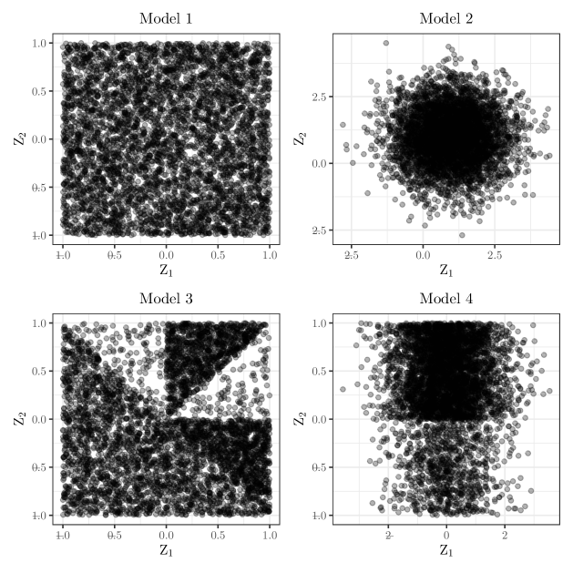
Figure 3: Scatterplots of a sample of size $n=5,000$ from the four models illustrate the joint distribution of $Z_{1}$ and $Z_{2}$. For models 1 and 2, parameter $d$ is set to 2 (two running variables). Joint density is continuous, and the condition in equation 23 is satisfied. For models 3 and 4, parameters $\gamma_{1}$ and $\gamma_{2}$ are 0.8: joint density is not continuous, and condition in equation 23 is not satisfied.

5.1 Model 1 and model 2

Model 1.

Consider $d$ running variables uniformly distributed:

$$Z_{j}\sim U(-1,1)\quad\text{for }j\text{ in }\{1,\dots,d\}.$$ (13)

In model 1, densities are symmetrical to the threshold, and the density function is flat. Since the setting can be particularly convenient for the tests, model 2 considers densities with different behaviors at the two sides of the boundary.

Model 2.

Consider $d$ running variables normally distributed and centered at 1:

$$Z_{j}\sim\mathcal{N}(1,1)\quad\text{for }j\text{ in }\{1,\dots,d\}.$$ (14)

Both models 1 and 2 are simulated considering sample sizes $n\in\{500,2000,5000\}$ and total numbers of running variables $d\in\{2,3,4\}$. The simulation results are presented in Table 2. Overall, for all the sample sizes considered, the tests tend to under-reject, with empirical rejection rates closer to the theoretical ones for DT and SDT. MT and BCT exhibit similar performances across different models and parameters specification: rejection rates get closer to asymptotic ones as the effective sample size grows, when $d$ decreases for a fixed $n$ or $n$ increases for a fixed $d$. For the same values of parameters $d$ and $n$, under-rejection is larger in model 1 than model 2: as expected, the steeper is the probability density function at the cutoff, the higher is the probability for the test to reject the true null.

Table 2: Rejection rates under the true null hypothesis of continuity of marginal densities of the running variables, computed through 5,000 Monte Carlo simulations, at 5% significance level. MT is the manipulation test proposed in this paper; BCT is the multiple hypotheses test with Bonferroni correction; DT and SDT consider as single running variables the Euclidean distance from the boundary: for SDT, running variables are standardized to have unitary variance before computing the distance, while for DT they are not. $d$ is the number of running variables, and $n$ is the sample size.

		Model 1				Model 2
$d$	$n$	MT	BCT	DT	SDT	MT	BCT	DT	SDT
2	500	$0.025$	$0.030$	$0.043$	$0.044$	$0.037$	$0.036$	$0.043$	$0.043$
	2,000	$0.036$	$0.039$	$0.047$	$0.046$	$0.042$	$0.041$	$0.050$	$0.049$
	5,000	$0.032$	$0.031$	$0.045$	$0.045$	$0.040$	$0.039$	$0.052$	$0.052$
3	500	$0.024$	$0.025$	$0.036$	$0.037$	$0.029$	$0.033$	$0.041$	$0.040$
	2,000	$0.027$	$0.029$	$0.041$	$0.040$	$0.038$	$0.039$	$0.039$	$0.039$
	5,000	$0.033$	$0.033$	$0.037$	$0.037$	$0.037$	$0.040$	$0.045$	$0.044$
4	500	$0.025$	$0.019$	$0.047$	$0.047$	$0.037$	$0.032$	$0.043$	$0.039$
	2,000	$0.020$	$0.019$	$0.041$	$0.040$	$0.036$	$0.036$	$0.042$	$0.042$
	5,000	$0.030$	$0.035$	$0.044$	$0.044$	$0.039$	$0.041$	$0.041$	$0.041$

Unsurprisingly, all the tests have a comparable performance: no theoretical reason suggests discrepancies for the three tests in controlling size. Differences arise when finite sample power is studied, as shown by models 3 and 4.

5.2 Model 3

Model 3.

Define random vector $Z^{*}=(Z_{1}^{*},Z_{2}^{*})$, where $Z_{1}^{*}\sim U(-1,1)$, $Z_{2}^{*}\sim U(-1,1)$, and $Z_{1}^{*}$ and $Z_{2}^{*}$ independent. Define sets $A_{1}=\{(z_{1},z_{2}):z_{1}<0,-z_{1}<z_{2}\}$ and $A_{2}=\{(z_{1},z_{2}):z_{1}>z_{2},z_{2}>0\}$.

Consider two running variables $Z_{1}$ and $Z_{2}$ distributed as follows:

$$Z_{1}\sim\begin{cases}Z_{1}^{*},&\text{if }Z^{*}\not\in A_{1}\\ Z_{1}^{*},&\text{with probability $1-\gamma_{1}$}\text{ if }Z^{*}\in A_{1}\\ -Z_{1}^{*},&\text{with probability $\gamma_{1}$}\text{ if }Z^{*}\in A_{1}\end{cases}$$ (15)

$$Z_{2}\sim\begin{cases}Z_{2}^{*},&\text{if }Z^{*}\not\in A_{2}\\ Z_{2}^{*},&\text{with probability $1-\gamma_{1}$}\text{ if }Z^{*}\in A_{2}\\ -Z_{2}^{*},&\text{with probability $\gamma_{1}$}\text{ if }Z^{*}\in A_{2}\end{cases}$$ (16)

Model 3 mimics a setting where the two running variables are manipulated, but in opposite directions: when $Z^{*}\in A_{1}$, $Z_{1}$ is manipulated to get the treatment; when $Z^{*}\in A_{2}$, $Z_{2}$ is manipulated to avoid the treatment. Parameter $\gamma_{1}$ governs the extent of manipulation: when $\gamma_{1}=0$, the joint density of $Z_{1}$ and $Z_{2}$ is continuous; when $\gamma_{1}=1$, the joint density becomes zero in regions $A_{1}$ and $A_{2}$, resulting in the maximum discontinuity.

The curves depicted in figure 4 illustrate the finite sample performance of the tests. For both MT and BCT, the power of the tests increases with the degree of manipulation $\gamma_{1}$, as expected. For DT and SDT, the power always remains equal to the test size. This design corresponds to the situation described in section 4.3: the condition in Proposition 1 is not satisfied, since neither the marginal densities of $Z_{1}$ nor $Z_{2}$ are continuous at the threshold (as shown in figure 3). Nonetheless, the probability density function of the distance from the boundary is continuous. Consequently, the null hypothesis tested by DT and SDT is true, resulting in trivial power for these tests.

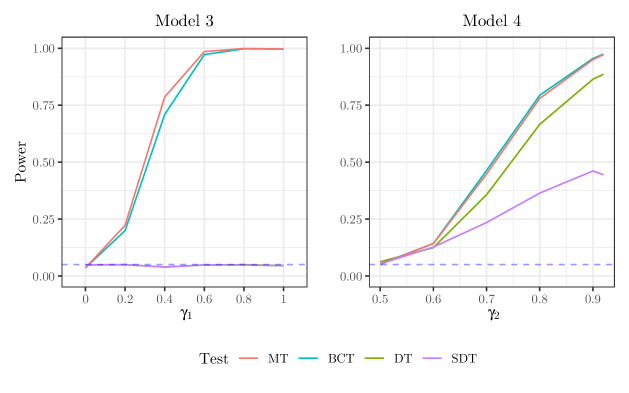
Figure 4: Power of different manipulation tests with $n=2,000$, computed though 5,000 Monte Carlo simulations. The dotted line indicates the nominal size of the tests (5%). MT is the manipulation test proposed in this paper; BCT is the multiple hypotheses test with Bonferroni correction; DT and SDT consider as single running variables the Euclidean distance from the boundary: for SDT, running variables are standardized to have unitary variance before computing the distance; for DT, they are not. Parameters $\gamma_{1}$ and $\gamma_{2}$ determine the degree of manipulation. In Model 3, lines for DT and SDT overlap.

5.3 Model 4

Model 4.

Consider two running variables distributed as follows:

$$Z_{1}\sim\mathcal{N}(0,1)$$ (17)

$$Z_{2}\sim\begin{cases}U(0,1),&\text{with probability $\gamma_{2}$}\\ U(-1,0),&\text{with probability $1-\gamma_{2}$}.\end{cases}$$ (18)

Model 4 is a design where only $Z_{2}$ is manipulated. The manipulation is determined by the parameter $\gamma_{2}$. When $\gamma_{2}=0.5$, $Z_{2}$ has a continuous density, following a uniform distribution between -1 and 1. When $\gamma_{2}=1$, the density of $Z_{2}$ becomes zero at the left of the boundary. The degree of discontinuity increases as the value of $Z_{2}$ deviates further from 0.5.

The curves in figure 4 show how the finite sample power depends on $\gamma_{2}$. The power increases with higher values of $\gamma_{2}$ for all tests, but it is lower for DT and SDT. Additionally, despite two similar versions of the same test, DT and SDT’s performances are different. As discussed in 4.3, the choice of the unit of measure affects the result of DT. In this case, the standardization applied in SDT reduces its power compared to DT. Standardization is not the solution to the issue.

It is noteworthy that MT and BCT exhibit similar behavior in the context of model 4, which mimics the second framework studied in the local asymptotic analysis, theoretically less favorable for MT.

Overall, the Monte Carlo simulations confirm that the manipulation test proposed in this paper has better finite sample properties than alternative tests. The simulations demonstrate advantages in terms of power and robustness, reinforcing the findings derived from the local asymptotic analysis discussed earlier.

Remarkably, the proposed manipulation test can be readily implemented using existing packages in popular statistical software, such as R and STATA. Users can conduct the manipulation test with just a few lines of code without selecting additional tuning parameters. This ease of implementation enhances the practical applicability of the test. The next section implements the manipulation test in a real-world application, illustrating its simplicity.

6 Application: frey2019cash

I apply my manipulation test for the MRDD considered by frey2019cash investigating the political economy of redistributive policies. In the original analysis, no manipulation test is reported. The paper studies the impact of cash transfers implemented by the Brazilian federal government on the dynamics of clientelism at the municipal level. The main hypothesis suggests that these cash transfers, by reducing the vulnerability of the poor, diminish the attractiveness of clientelism as a strategy for incumbent mayors.

The Bolsa Família (BF) program is the largest conditional cash transfer program globally and has been implemented in households across Brazil since 2003. The coverage of BF across different municipalities exhibits a positive correlation with the funding allocated to the Family Health Program (FHP), a household-based healthcare program run by municipalities since 1995. The positive correlation between BF coverage and FHP funding can be attributed to the fact that FHP teams have a significant penetration among the poor households, potential beneficiaries of BF. This enables them to effectively disseminate information about the BF program and encourage enrollment among eligible households.

To estimate the causal effect of the cash transfers on local clientelism, frey2019cash exploits the link between BF and FHP, along with a specific discontinuity in the design of the FHP. The FHP provides municipalities with an additional 50% funding if they meet two criteria: a population of fewer than 30,000 inhabitants and a Human Development Index (HDI) below 0.70. This discontinuity, determined by the joint thresholds of population and HDI, is directly reflected in the diffusion of the BF program: consequences of cash transfers can be analyzed using an MRDD.

Figure 5 provides a visualization of the MRDD. In the space of the two running variables (population and HDI), treated municipalities are depicted in light blue, and untreated municipalities in dark blue. The red line represents the boundary. In this specific context, the treatment corresponds to the additional FHP funding, which leads to variations in the adoption rate of the BF program.

In this context, the MRDD requires the assumption that the joint density of population and HDI is continuous at the boundary, thereby ensuring the continuity of their respective marginal densities. The manipulation test is employed to validate the design and enhance the credibility of the study’s findings. The test is run considering two running variables, resulting in a p-value of 0.490. With a significance level of $\alpha=0.05$, the null hypothesis is not rejected, indicating no evidence of manipulation.

It is important to emphasize that the manipulation test alone does not establish the model’s validity. It serves as a robustness check and provides supporting evidence for the continuity of the densities of the running variables, which is a necessary condition for Assumptions 1 and 2. It cannot substitute a discussion on why Assumptions 1 and 2 are likely to hold in this setting, a discussion that remains essential for drawing valid conclusions from the analysis.

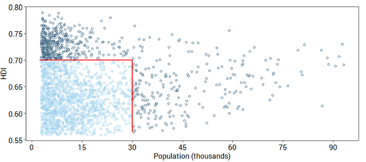
Figure 5: Running variables for the MRDD considered by frey2019cash. Municipalities are assigned to the policy (light blue dots) when the population is below 30,000 inhabitants (x-axis), and Human Development Index is below 0.7 (y-axis).

7 Conclusion

This paper introduced a manipulation test for the multidimensional regression discontinuity design. Like the single-dimensional RDD developed by lee2008randomized, I constructed a causal inference model for the MRDD. From an assumption on unobservable agents’ behavior, I derived an implication on observable quantities—the continuity of the conditional marginal densities of the multiple running variables. I proposed a manipulation test for the implication, which was then compared with alternative approaches commonly used in applied research. While these approaches vary, they generally lack clear theoretical justification, and some are inconsistent for the considered implication. Through Monte Carlo simulations and local power analysis, I explored the finite sample properties of the tests.

The manipulation test should be seen as a robustness check to strengthen the credibility of the assumptions required by the MRDD, and it is not intended as a pre-test. It can be readily implemented with already existing packages without the need for additional tuning parameters. Considering the application in frey2019cash, I showed how to use the test in practice.

Appendix A Formulas for $B(x)$, $V(x)$, and $\hat{V}(x)$

Formulas for $B(x)$, $V(x)$, and $\hat{V}(x)$ are derived by cattaneo2020simple.

Let $x_{L}$ and $x_{U}$ indicate the lower and the upper bound of the support of $X$: the support does not need to be bounded, and they can be $-\infty$ and $\infty$. First, define the following:

$$A(x)= f(x)\int_{\frac{x_{L}-x}{h}}^{\frac{x_{U}-x}{h}}r_{p}(u)r_{p}(u)^{\prime}K(u)du$$

$$a(x)= f(x)\frac{F^{(p+1)}(x)}{(p+1)!}\int_{\frac{x_{L}-x}{h}}^{\frac{x_{U}-x}{h}}u^{p+1}r_{p}(u)K(u)du$$

$$C(x)= f(x)^{3}\int_{\frac{x_{L}-x}{h}}^{\frac{x_{U}-x}{h}}\int_{\frac{x_{L}-x}{h}}^{\frac{x_{U}-x}{h}}\min\{u,v\}r_{p}(u)r_{p}(v)^{\prime}K(u)K(v)dudv.$$

with $A(x)\in\mathbb{R}^{(p+1)\times(p+1)}$, $a(x)\in\mathbb{R}^{(p+1)}$, $C(x)\in\mathbb{R}^{(p+1)\times(p+1)}$. Bias $B(x)$ and variance $V(x)$ are:

$$B(x) =e_{1}^{\prime}A(x)^{-1}a(x)$$

$$V(x) =e_{1}^{\prime}A(x)^{-1}C(x)A(x)^{-1}e_{1}.$$

Consider the following estimators for $A(x)$ and $C(x)$:

$$\hat{A}(x)= \frac{1}{nh}\sum_{i=1}^{n}r_{p}\left(\frac{x_{i}-x}{h}\right)r_{p}\left(\frac{x_{i}-x}{h}\right)^{\prime}K\left(\frac{x_{i}-x}{h}\right)$$

$$\hat{C}(x)= \frac{1}{n^{3}h^{3}}\sum_{i,j,k=1}^{n}r_{p}\left(\frac{x_{j}-x}{h}\right)r_{p}\left(\frac{x_{k}-x}{h}\right)^{\prime}K\left(\frac{x_{j}-x}{h}\right)K\left(\frac{x_{k}-x}{h}\right)$$

$$\left[\mathbf{1}\{x_{i}\leq x_{j}\}-\hat{F}(x_{j})\right]\left[\mathbf{1}\{x_{i}\leq x_{k}\}-\hat{F}(x_{k})\right]$$

and then the estimator for $V(x)$:

$$\hat{V}_{p}(x) =e_{1}^{\prime}\hat{A}(x)^{-1}\hat{C}(x)\hat{A}(x)^{-1}e_{1}.$$

Consistency of $\hat{V}_{p}(x)$ for $V(x)$ is proved in Theorem 2 in cattaneo2020simple.

Appendix B Test with the max-statistic

Corollary 1 derives the asymptotic distribution of any continuous function $g$ applied to the statistic $\hat{\Sigma}^{-\frac{1}{2}}\hat{\theta}$. However, not all statistics of the form $g(\hat{\Sigma}^{-\frac{1}{2}}\hat{\theta})$ can be employed to construct a valid manipulation test. Corollary 2 demonstrates that the quadratic form $\hat{t}$ ensures a consistent test. Similarly, one can establish the consistency of the manipulation test $\phi_{m}(\hat{t}_{m},\alpha)$ defined as follows:

$$\phi_{m}(\hat{t}_{m},\alpha)=\begin{cases}1,&\text{if $\hat{t}_{m}>c_{m}(\alpha)$}\\ 0,&\text{if $\hat{t}_{m}\leq c_{m}(\alpha)$}.\end{cases}$$ (19)

Here, $\hat{t}_{m}$ is the max-statistic $\hat{t}_{m}=\max\left(|\frac{\hat{\theta}_{1}}{\hat{\sigma}_{1}}|,\dots,|\frac{\hat{\theta}_{d}}{\hat{\sigma}_{d}}|\right)$, and the critical value $c_{m}(\alpha)$ is the $1-\alpha$ quantile of the distribution of $\max\left(|X_{1}|,\dots,|X_{d}|\right)$, where $X\sim\mathcal{N}(0,I_{d})$.

Both MT (the manipulation test using the quadratic form $\hat{t}$ as test statistic) and $\phi_{m}$ are consistent tests for the implication in Proposition 1, but their power against alternative hypotheses differs. The MT considers an average of statistics $\frac{\hat{\theta}_{j}}{\hat{\sigma}_{j}}$, and is hence better at rejecting the null hypothesis when manipulation is spread across all the running variables. Taking the maximum over $|\frac{\hat{\theta}_{j}}{\hat{\sigma}_{j}}|$, instead, $\phi_{m}$ has greater power when manipulation occurs for only one running variable.

My analysis in section 4.2 considered such a case, where manipulation happens for only one running variable. The plot in the bottom right corner of Figure 2 shows how, in these circumstances, the BCT (multiple tests with Bonferroni corrections) outperforms my manipulation test MT. In this case, though, the version of my test $\phi_{m}$ dominates the BCT, as shown in Figure B.1, where I reproduced the previous plot adding the power curve for $\phi_{m}$. Once again, a manipulation test that aggregates information from all the running variables testing a unique hypothesis is better than considering separate tests for each $\hat{\theta}_{j}$ accounting for multiple tests.

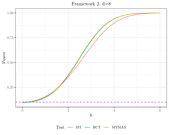
Figure B.1: Local asymptotic power curves for the manipulation test proposed in this paper (MT, in red) and the multiple hypotheses test with Bonferroni correction (BCT, in blue), and the manipulation test $\phi_{m}$ considering the max-statistic (MTMAX, in yellow). The dotted horizontal purple line represents the significance level $\alpha=0.1$. The data distribution is such that only running variable $j=1$ is discontinuous, and $\hat{\theta}_{1}\rightarrow^{d}\mathcal{N}(k,1)$ and $\hat{\theta}_{j}\rightarrow^{d}\mathcal{N}(0,1)$ for $j\neq 1$.

Appendix C Proofs

Theorem 1

Theorem 1.

(Identification of $\tau(b)$ and $\tau$) Under Assumptions 1 and 2, $\tau(b)$ and $\tau$ are identified.

Proof.

First, prove that $\mathbb{E}[Y_{0}|Z=z]$ and $\mathbb{E}[Y_{1}|Z=z]$ are continuous at $z=b\in\mathcal{B}$, where the expectation is taken with respect to random variables $W$, $Z$, and $y_{0}(w,z)$ and $y_{1}(w,z)$. Consider $\mathbb{E}[Y_{0}|Z=z]$:

$$\mathbb{E}[Y_{0}|Z=z]= \mathbb{E}[y_{0}(W,Z)|Z=z]=\int_{\mathcal{W}}\mathbb{E}[y_{0}(w,z)]f(w|z)dw=$$ (20)

$$= \int_{\mathcal{W}}\mathbb{E}[y_{0}(w,z)]f(z|w)\frac{g(w)}{f(z)}dw=$$ (21)

$$= \int_{\mathcal{W}}\mathbb{E}[y_{0}(w,z)]f(z|w)\frac{g(w)}{\int_{\mathcal{W}}f(z|w)g(w)dw}dw.$$ (22)

By assumption 1, $f(z|w)$ is continuous at $z=b\in\mathcal{B}$, and by assumption 2, $\mathbb{E}[y_{0}(w,z)]$ is continuous at $z=b\in\mathcal{B}$. Hence, $\mathbb{E}[Y_{0}|Z=z]$ is continuous at $z=b\in\mathcal{B}$. The proof for $\mathbb{E}[Y_{1}|Z=z]$ is analogous.

For any $b\in\mathcal{B}$, the Conditional Average Treatment Effect can be written as

$$\tau(b)= \mathbb{E}[Y_{1}-Y_{0}|Z=b]=\mathbb{E}[Y_{1}|Z=b]-\mathbb{E}[Y_{0}|Z=b]=$$

$$= \lim_{z\rightarrow b}\mathbb{E}[Y_{1}|Z=z]-\lim_{z\rightarrow b}\mathbb{E}[Y_{0}|Z=z]=$$

$$= \lim_{z\rightarrow b,z\in\mathcal{T}}\mathbb{E}[Y|Z=z]-\lim_{z\rightarrow b,z\in\mathcal{T^{C}}}\mathbb{E}[Y|Z=z].$$

In the last expression, the limits for $z\rightarrow b$ of $\mathbb{E}[Y|Z=z]$ are taken considering any sequence of $z\in\mathcal{T}$ and $z\in\mathcal{T^{C}}$. The last equality comes from the fact that, for sequences in $\mathcal{T}$, $Y=Y_{1}$, and for sequences in $\mathcal{T^{C}}$, $Y=Y_{0}$.

$Y$ and $Z$ are observable, and hence $\tau(b)$ is identified.

The Integrated Conditional Average Treatment Effect is then identified as

$$\tau=\int_{b\in\mathcal{B}}\tau(b)f(b|Z\in\mathcal{B})db=\frac{\int_{b\in\mathcal{B}}\tau(b)f(b)db}{\int_{b\in\mathcal{B}}f(b)db}.$$

∎

Proposition 1

Proposition 1.

(Testable implication) Assumption 1 implies the following condition on observable quantities:

$$f_{Z_{j}|Z_{-j}}(z_{j}|z_{-j}\geq 0)\text{ continuous at }z_{j}=0,\forall j.$$ (23)

Proof.

Consider the density of $Z$, $f(Z)$, that can be written as $f(z)=\int_{\mathcal{W}}f(z|w)g(w)dw$.

By assumption 1, $f(z|w)$ is continuous at $z=b\in\mathcal{B}$, and hence $f(z)\text{ is continuous at }z=b,\forall b\in\mathcal{B}$. The implication is not sharp: $f(z)$ may be continuous even if $f(z|w)$ is not (see lee2008randomized for a further discussion on this issue, which analogously arises in the single-dimensional case).

For any $j$, let $f_{-j}(z_{-j})$ be the joint density of $z_{-j}=(z_{1},\dots,z_{j-1},z_{j+1},\dots,z_{d})\in\mathbb{R}^{d-1}$. By definition of conditional density:

$$f_{Z_{j}|Z_{-j}}(z_{j}|z_{-j})=\frac{f_{Z_{j},Z_{-j}}(z_{j},z_{-j})}{f_{-j}(z_{-j})}=\frac{f(z)}{f_{-j}(z_{-j})}$$ (24)

and since $f(z)$ is continuous in $z$ and hence in $z_{j}$ at all $b\in\mathcal{B}$, so it is $f_{Z_{j}|Z_{-j}}(z_{j}|z_{-j})$. Whenever $z_{-j}\geq 0$, $f_{Z_{j}|Z_{-j}}(z_{j}|z_{-j})$ is continuous at $z_{j}=0$, as the set $\{z:z_{j}=0,z_{-j}\geq 0\}$ is a subset of $\mathcal{B}$.

By definition of conditional density, $f_{Z_{j}|Z_{-j}}(z_{j}|z_{-j}\geq 0)=\int_{z_{-j}\geq 0}f_{Z_{j}|Z_{-j}}(z_{j}|z_{-j})f_{-j}(z_{-j})dz_{-j}$: the previous result implies the right-hand side to be continuous at $z_{j}=0$. This gives the following implication:

$$f_{Z_{j}|Z_{-j}}(z_{j}|z_{-j}\geq 0)\text{ continuous at }z_{j}=0,\forall j.$$ (25)

∎

Proposition 2

Proposition 2.

(Asymptotic distribution of $\hat{f}_{j,p}(z_{j})$) Under Assumptions 1, 3 and 4, with $p=2$, $nh_{j}^{2}\rightarrow\infty$ and $nh_{j}^{2p+1}=O(1)$, $\hat{f}_{j,p}(z_{j})$ is a consistent estimator for $f_{j}(z_{j})$. Furthermore,

$$\sqrt{n_{j}h_{j}}(\hat{f}_{j,p}(z_{j})-f_{j}(z_{j})-h_{j}^{p}B(z_{j}))\rightarrow^{d}\mathcal{N}(0,V(z_{j}))$$ (26)

where $B(z_{j})$ is the asymptotic bias.

Proof.

The sample size $n_{j}$ considered by the estimator $\hat{f}_{j,p}(z_{j})$ is random. By the law of large numbers, $\frac{n_{j}}{n}=\frac{\sum_{i=1}^{n}\mathbf{1}\{z_{-j}\geq 0\}}{n}\rightarrow^{a.s.}\pi_{j}>0$, and hence $n_{j}\rightarrow\infty$ with probability 1. With probability 1, then, the proposition is equivalent to the one stated and proved as Theorem 1 in cattaneo2020simple.

Their results apply since $\hat{f}_{j,p}(z_{j})$ can be written as

$$\hat{f}_{j,p}(z_{j})=e_{1}^{\prime}\hat{\beta}(z_{j})$$

$$\hat{\beta}(z_{j})=\text{argmin}_{b\in\mathbb{R}^{p+1}}\sum_{i=1}^{n_{j}}\left[\tilde{F_{j}}(z_{j})-r_{p}(z_{ji}-z_{j})^{\prime}b\right]^{2}K\left(\frac{z_{ji}-z_{j}}{h_{j}}\right)$$

if only observations with $z_{-j}\geq 0$ are considered, with $n_{j}\rightarrow\infty$ with probability 1, $n_{j}h_{j}^{2}\rightarrow\infty$ and $n_{j}h_{j}^{2p+1}=O(1)$. ∎

Proposition 3

Proposition 3.

(Asymptotic distribution of $\hat{\theta}_{j,q}$) Under Assumptions 1, 3 and 4 holding separately for $\{Z:Z\geq 0\}$ and $\{Z:Z_{-j}\geq 0,Z_{j}<0\}$, with $p=2$, $q=p+1$, $n\min\{h_{j-},h_{j+}\}\rightarrow\infty$, and $n\max\{h_{j-}^{1+2q},h_{j+}^{1+2q}\}\rightarrow 0$, when the implication $\theta_{j}=0$ is true:

$$\frac{1}{\sigma_{j}}\hat{\theta}_{j,q}\rightarrow^{d}\mathcal{N}\left(0,1\right)$$ (27)

where

$$\sigma_{j}^{2}=\frac{\pi_{j+}}{h_{j+}\pi_{j}n}V_{j+}(0)+\frac{\pi_{j-}}{h_{j-}\pi_{j}n}V_{j-}(0).$$ (28)

A consistent estimator $\hat{\sigma}_{j}^{2}$ for $\sigma_{j}^{2}$ can be obtained by

$$\hat{\sigma}_{j}^{2}=\frac{n_{j+}}{h_{j+}n_{j}^{2}}\hat{V}_{j+,q}(0)+\frac{n_{j-}}{h_{j-}n_{j}^{2}}\hat{V}_{j-,q}(0).$$ (29)

Proof.

As for Proposition 2, the effective samples sizes $n_{j}$, $n_{j+}$ and $n_{j-}$ are stochastic. By the law of large numbers, $\frac{n_{j}}{n}\rightarrow^{a.s.}\pi_{j}>0$, $\frac{n_{j+}}{n_{j}}\rightarrow^{a.s.}\pi_{j+}>0$, and $\frac{n_{j-}}{n_{j}}\rightarrow^{a.s.}\pi_{j-}>0$, and hence $n_{j}\rightarrow\infty$, $n_{j+}\rightarrow\infty$, and $n_{j-}\rightarrow\infty$ with probability 1. Then, with probability 1, this proposition is equivalent to the result stated and proved as Corollary 1 in the appendix of cattaneo2020simple.

Since $\hat{V}_{j+,q}(0)\to^{p}V_{j+}(0)$, $\hat{V}_{j-,q}(0)\to^{p}V_{j+}(0)$, $\frac{n_{j+}}{h_{j+}n_{j}^{2}}\to^{p}\frac{\pi_{j+}}{h_{j+}\pi_{j}n}$, and $\frac{n_{j-}}{h_{j-}n_{j}^{2}}\to^{p}\frac{\pi_{j-}}{h_{j-}\pi_{j}n}$, the Slutsky theorem implies $\hat{\sigma}_{j}^{2}\to^{p}\sigma_{j}^{2}$. ∎

Theorem 2

Theorem 2.

(Asymptotic distribution of $\hat{\theta}$) Under Assumptions 1, 3 and 4 holding separately for $\{Z:Z\geq 0\}$ and $\{Z:Z_{-j}\geq 0,Z_{j}<0\}$ for all $j$, with $p=2$, $q=p+1$, $n\min\{h_{j-},h_{j+}\}\rightarrow\infty$ and $n\max\{h_{j-}^{1+2q},h_{j+}^{1+2q}\}\rightarrow 0$ for all $j$, when $\theta=0$,

$$\hat{\Sigma}^{-\frac{1}{2}}\hat{\theta}\rightarrow^{d}\mathcal{N}(0,I).$$

where $\hat{\Sigma}_{jj}=\hat{\sigma}^{2}_{j}$ as defined in Proposition 3, and $\hat{\Sigma}_{ji}=0$ for all $i\neq j$.

Proof.

Proposition 3 derives the univariate asymptotic distribution of $\frac{1}{\sigma_{j}}\hat{\theta}_{j}$. Consider any pair of elements of $\hat{\Sigma}^{-\frac{1}{2}}\hat{\theta}$. Showing that they are asymptotically independent proves the theorem, as independent normal distributions are jointly normal.

Without loss of generality, consider $\frac{1}{\hat{\sigma_{1}}}\hat{\theta}_{1}$ and $\frac{1}{\hat{\sigma_{2}}}\hat{\theta}_{2}$, where:

$$\hat{\theta}_{1,p}=\frac{n_{1+}}{n_{1}}\hat{f}_{1+,p}(0)-\frac{n_{1-}}{n_{1}}\hat{f}_{1-,p}(0)$$ (30)

$$\hat{\theta}_{2,p}=\frac{n_{2+}}{n_{2}}\hat{f}_{2+,p}(0)-\frac{n_{2-}}{n_{2}}\hat{f}_{2-,p}(0).$$ (31)

In finite samples, $\hat{\theta}_{1,p}$ and $\hat{\theta}_{2,p}$ are not independent: $\hat{f}_{1+,p}(0)$ and $\hat{f}_{2+,p}(0)$ are computed with different but overlapping sets of observations. For an intuition, consider the bi-dimensional space of the two running variables: each estimator gives non-zero weights to observations in a stripe of width $h_{1+}$ or $h_{2+}$ close to the boundary. Close to the origin, the stripes overlap. $\hat{f}_{1+,p}(0)$ and $\hat{f}_{2+,p}(0)$ considers a number of observations proportional to $n_{1+}h_{1+}$ and $n_{1+}h_{2+}$, while the shared number is proportional to $n_{1+}h_{1+}h_{2+}$. Note that, under the assumptions on rates of convergence, $n_{1+}h_{1+}h_{2+}\rightarrow\infty$.

Write $\frac{1}{\hat{\sigma_{1}}}\hat{\theta}_{1}$ as:

$$\frac{1}{\hat{\sigma_{1}}}\hat{\theta}_{1}=\left(\frac{1}{n_{1}h_{1+}}\frac{n_{1+}}{n_{1}}\hat{V}_{1+,q}(0)+\frac{1}{n_{1}h_{1-}}\frac{n_{1-}}{n_{1}}\hat{V}_{1-,q}(0)\right)^{-\frac{1}{2}}\hat{\theta}_{1}=$$ (32)

$$\frac{n_{1}}{n_{1+}}\underbrace{\frac{n_{1+}}{n_{1}}\left(\frac{n_{1+}h_{1+}}{n_{1}h_{1+}}\frac{n_{1+}}{n_{1}}\hat{V}_{1+,q}(0)+\frac{n_{1+}h_{1+}}{n_{1}h_{1-}}\frac{n_{1-}}{n_{1}}\hat{V}_{1-,q}(0)\right)^{-\frac{1}{2}}}_{\hat{M}_{n_{1}}}(n_{1+}h_{1+})^{\frac{1}{2}}\hat{\theta}_{1}.$$ (33)

To prove asymptotic independence of $\frac{n_{1}}{n_{1+}}\hat{M}_{n_{1}}(n_{1+}h_{1+})^{\frac{1}{2}}\hat{\theta}_{1}$ and $\frac{n_{2}}{n_{2+}}\hat{M}_{n_{2}}(n_{2+}h_{2+})^{\frac{1}{2}}\hat{\theta}_{2}$, I need to show that $\hat{M}_{n_{1}}(n_{1+}h_{1+})^{\frac{1}{2}}\hat{f}_{1+,p}(0)$ and $\hat{M}_{n_{2}}(n_{2+}h_{2+})^{\frac{1}{2}}\hat{\hat{f}}_{2+,p}(0)$ are independent.

Define $\hat{f}_{1+,p}^{*}(0)$ and $\hat{M}_{n_{1}}^{*}$ as the estimators analogous to $\hat{f}_{1+,p}(0)$ and $\hat{M}_{n_{1}}$ that consider only observations not in the overlapping region. I will show that $|\hat{M}_{n_{1}}(n_{1+}h_{1})^{\frac{1}{2}}\hat{f}_{1+,p}(0)-\hat{M}_{n_{1}}^{*}(n_{1+}h_{1})^{\frac{1}{2}}\hat{f}_{1+,p}^{*}(0)|\rightarrow 0$, and prove the theorem, since $\hat{f}_{1+,p}^{*}(0)$ and $\hat{f}_{2+,p}(0)$, and $\hat{M}_{n_{1}}^{*}$ and $\hat{M}_{n_{2}}$, are independent.

In the proof, where not necessary, I omit the subscripts $+$ and $p$, and the argument $z_{j}=0$, and consider vector $\hat{\beta}_{j}$, where $\hat{f}_{j+,p}^{*}(z_{j})=e_{1}^{\prime}\hat{\beta}_{j}(z_{j})$. The local linear estimator can be written in the matrix form:

$$\hat{\beta}_{j}=H^{-1}(X^{\prime}KX)^{-1}X^{\prime}KY$$ (34)

where

$$H=\text{diag}\left(h_{j}^{0},h_{j}^{1},\dots,h_{j}^{p}\right)$$

$$X=\left[\left(\frac{z_{ji}}{h_{j}}\right)^{m}\right]_{1\leq i\leq n_{j},0\leq m\leq p}$$

$$K=\text{diag}\left(\left[\frac{1}{h_{j}}K\left(\frac{z_{ji}}{h_{j}}\right)\right]_{1\leq i\leq n_{j+}}\right)$$

$$Y=\left(\tilde{F}_{j}(z_{ji})\right)_{1\leq i\leq n_{j}}$$

Matrices $X$ and $Y$ can be decomposed as $X=A+B$ and $Y=C+D$, where $A$ and $C$ have rows of zeros in correspondence with the overlapping observations. In contrast, $B$ and $D$ have rows of zero in correspondence of non-overlapping ones. Note that

$$\sqrt{n_{j}h_{j}}\hat{\beta}_{j}=\sqrt{n_{j}h_{j}}H^{-1}(A^{\prime}KA+B^{\prime}KB)^{-1}(A^{\prime}KC+B^{\prime}KD)=$$ (35)

$$H^{-1}\left(\underbrace{\frac{(n_{j}-n_{j}h_{j})h_{j}}{n_{j}h_{j}}}_{\rightarrow 1}\underbrace{\frac{1}{(n_{j}-n_{j}h_{j})h_{j}}A^{\prime}KA}_{\rightarrow^{p}O(1)}+\underbrace{\frac{n_{j}h_{j}^{2}}{n_{j}h_{j}}}_{\rightarrow 0}\underbrace{\frac{1}{n_{j}h_{j}^{2}}B^{\prime}KB}_{\rightarrow^{p}O(1)}\right)^{-1}$$ (36)

$$\left(\underbrace{\frac{\sqrt{(n_{j}-n_{j}h_{j})h_{j}}}{\sqrt{n_{j}h_{j}}}}_{\rightarrow 1}\underbrace{\frac{1}{\sqrt{(n_{j}-n_{j}h_{j})h_{j}}}A^{\prime}KC}_{\rightarrow^{p}O(1)}+\underbrace{\frac{\sqrt{n_{j}h_{j}^{2}}}{\sqrt{n_{j}h_{j}}}}_{\rightarrow 0}\underbrace{\frac{1}{\sqrt{n_{j}h_{j}^{2}}}B^{\prime}KD}_{\rightarrow^{p}O(1)}\right)$$ (37)

$$\rightarrow\sqrt{n_{j}h_{j}}H^{-1}(A^{\prime}KA)^{-1}(A^{\prime}KC)=\sqrt{n_{j}h_{j}}\hat{\beta}_{j}^{*}$$ (38)

This demonstrates that $\left|\sqrt{n_{j}h_{j}}\hat{\beta}_{j}-\sqrt{n_{j}h_{j}}\hat{\beta}_{j}^{*}\right|\rightarrow 0$. Analogously, it can be shown that $\hat{M}_{n_{1}}\rightarrow M_{1}$ and $\hat{M}_{n_{1}}^{*}\rightarrow M_{1}$, with $M_{1}=\pi_{1+}\left(\pi_{1+}^{2}V_{1+,q}(0)+\pi_{1+}\pi_{1-}\frac{h_{1+}}{h_{1-}}V_{1-,q}(0)\right)^{-\frac{1}{2}}$. The result is hence obtained:

$$\left|\hat{M}_{n_{1}}(n_{j+}h_{j})^{\frac{1}{2}}\hat{f}_{1+,p}(0)-\hat{M}_{n_{1}}^{*}(n_{j+}h_{j})^{\frac{1}{2}}\hat{f}_{1+,p}^{*}(0)\right|\rightarrow 0.$$

Since $\hat{\theta}_{j}$ and $\hat{\theta}_{i}$ are asymptotically independent, $\hat{\Sigma}_{ji}=0$ for all $j\neq i$. ∎

Corollary 2

Corollary 3.

(Manipulation test) Let $H_{0}$ be the null hypothesis reported in equation 23. Under the assumptions of Theorem 2, when $H_{0}$ is true:

$$\lim_{n\rightarrow\infty}P(\phi(\hat{t},\alpha)=1)=\alpha.$$ (39)

When $H_{0}$ is false:

$$\lim_{n\rightarrow\infty}P(\phi(\hat{t},\alpha)=1)=1.$$ (40)

Proof.

The proof for the case of true null hypothesis immediately follows from Theorem 2: asymptotically, $\hat{\Sigma}^{-\frac{1}{2}}\hat{\theta}$ is distributed as a multinomial standard normal, and hence the quadratic form $\hat{t}$ is such that $\hat{t}=\hat{\theta}^{\prime}\hat{\Sigma}^{-1}\hat{\theta}\rightarrow^{d}\chi^{2}_{d}$.

For the case when $H_{0}$ is false, note that it means that at least one of the conditional marginal densities is not continuous: it exists a $j$ such that $\theta_{j}\neq 0$, and hence $\frac{1}{\hat{\sigma}_{j}}\hat{\theta}_{j,q}\to\infty$. It implies $\hat{t}\to\infty$, and then $\lim_{n\rightarrow\infty}P(\phi(\hat{t},\alpha)=1)=1$. ∎

References

- Abadie and Cattaneo (2018) Abadie, A. and M. D. Cattaneo (2018). Econometric methods for program evaluation. Annual Review of Economics 10(1).
- Abdulkadiroglu et al. (2022) Abdulkadiroglu, A., J. D. Angrist, Y. Narita, and P. Pathak (2022). Breaking ties: Regression discontinuity design meets market design. Econometrica 90(1), 117–151.
- Armstrong and Kolesár (2020) Armstrong, T. B. and M. Kolesár (2020). Simple and honest confidence intervals in nonparametric regression. Quantitative Economics 11(1), 1–39.
- Becht et al. (2016) Becht, M., A. Polo, and S. Rossi (2016). Does mandatory shareholder voting prevent bad acquisitions? The Review of financial studies 29(11), 3035–3067.
- Bugni and Canay (2021) Bugni, F. A. and I. A. Canay (2021). Testing continuity of a density via g-order statistics in the regression discontinuity design. Journal of Econometrics 221(1), 138–159.
- Calonico et al. (2018) Calonico, S., M. D. Cattaneo, and M. H. Farrell (2018). On the effect of bias estimation on coverage accuracy in nonparametric inference. Journal of the American Statistical Association 113(522), 767–779.
- Calonico et al. (2022) Calonico, S., M. D. Cattaneo, and M. H. Farrell (2022). Coverage error optimal confidence intervals for local polynomial regression. Bernoulli 28(4), 2998–3022.
- Canay and Kamat (2018) Canay, I. A. and V. Kamat (2018). Approximate permutation tests and induced order statistics in the regression discontinuity design. The Review of Economic Studies 85(3), 1577–1608.
- Cattaneo et al. (2019a) Cattaneo, M. D., N. Idrobo, and R. Titiunik (2019a). A practical introduction to regression discontinuity designs: Extensions. Cambridge University Press.
- Cattaneo et al. (2019b) Cattaneo, M. D., N. Idrobo, and R. Titiunik (2019b). A practical introduction to regression discontinuity designs: Foundations. Cambridge University Press.
- Cattaneo et al. (2020) Cattaneo, M. D., M. Jansson, and X. Ma (2020). Simple local polynomial density estimators. Journal of the American Statistical Association 115(531), 1449–1455.
- Cattaneo et al. (2022) Cattaneo, M. D., M. Jansson, and X. Ma (2022). lpdensity: Local polynomial density estimation and inference. Journal of Statistical Software 101(2), 1–25.
- Clark and Martorell (2014) Clark, D. and P. Martorell (2014). The signaling value of a high school diploma. Journal of Political Economy 122(2), 282–318.
- Cohodes and Goodman (2014) Cohodes, S. R. and J. S. Goodman (2014). Merit aid, college quality, and college completion: Massachusetts’ adams scholarship as an in-kind subsidy. American Economic Journal: Applied Economics 6(4), 251–85.
- Egger and Wamser (2015) Egger, P. H. and G. Wamser (2015). The impact of controlled foreign company legislation on real investments abroad. a multi-dimensional regression discontinuity design. Journal of Public Economics 129, 77–91.
- Elacqua et al. (2016) Elacqua, G., M. Martinez, H. Santos, and D. Urbina (2016). Short-run effects of accountability pressures on teacher policies and practices in the voucher system in santiago, chile. School Effectiveness and School Improvement 27(3), 385–405.
- Evans (2017) Evans, B. J. (2017). Smart money: Do financial incentives encourage college students to study science? Education Finance and Policy 12(3), 342–368.
- Fan and Gijbels (1996) Fan, J. and I. Gijbels (1996). Local polynomial modelling and its applications. Chapman and Hall, London.
- Frey (2019) Frey, A. (2019). Cash transfers, clientelism, and political enfranchisement: Evidence from brazil. Journal of Public Economics 176, 1–17.
- Hinnerich and Pettersson-Lidbom (2014) Hinnerich, B. T. and P. Pettersson-Lidbom (2014). Democracy, redistribution, and political participation: Evidence from sweden 1919–1938. Econometrica 82(3), 961–993.
- Imbens and Wager (2019) Imbens, G. and S. Wager (2019). Optimized regression discontinuity designs. Review of Economics and Statistics 101(2), 264–278.
- Imbens and Zajonc (2009) Imbens, G. and T. Zajonc (2009). Regression discontinuity design with vector-argument assignment rules. Unpublished paper.
- Jones (1993) Jones, M. C. (1993). Simple boundary correction for kernel density estimation. Statistics and computing 3(3), 135–146.
- Keele and Titiunik (2015) Keele, L. J. and R. Titiunik (2015). Geographic boundaries as regression discontinuities. Political Analysis 23(1), 127–155.
- Lee (2008) Lee, D. S. (2008). Randomized experiments from non-random selection in us house elections. Journal of Econometrics 142(2), 675–697.
- Lehmann and Romano (2022) Lehmann, E. L. and J. P. Romano (2022). Testing statistical hypotheses (4th edition). Springer.
- Londoño-Vélez et al. (2020) Londoño-Vélez, J., C. Rodríguez, and F. Sánchez (2020). Upstream and downstream impacts of college merit-based financial aid for low-income students: Ser pilo paga in colombia. American Economic Journal: Economic Policy 12(2), 193–227.
- Matsudaira (2008) Matsudaira, J. D. (2008). Mandatory summer school and student achievement. Journal of Econometrics 142(2), 829–850.
- McCrary (2008) McCrary, J. (2008). Manipulation of the running variable in the regression discontinuity design: A density test. Journal of econometrics 142(2), 698–714.
- Narita and Yata (2021) Narita, Y. and K. Yata (2021). Algorithm is experiment: Machine learning, market design, and policy eligibility rules. arXiv preprint arXiv:2104.12909.
- Papay et al. (2011) Papay, J. P., J. B. Willett, and R. J. Murnane (2011). Extending the regression-discontinuity approach to multiple assignment variables. Journal of Econometrics 161(2), 203–207.
- Salti et al. (2022) Salti, N., J. Chaaban, W. Moussa, A. Irani, R. Al Mokdad, Z. Jamaluddine, and H. Ghattas (2022). The impact of cash transfers on syrian refugees in lebanon: Evidence from a multidimensional regression discontinuity design. Journal of Development Economics 155, 102803.
- Smith et al. (2017) Smith, J., M. Hurwitz, and C. Avery (2017). Giving college credit where it is due: Advanced placement exam scores and college outcomes. Journal of Labor Economics 35(1), 67–147.
- Snider and Williams (2015) Snider, C. and J. W. Williams (2015). Barriers to entry in the airline industry: A multidimensional regression-discontinuity analysis of air-21. Review of Economics and Statistics 97(5), 1002–1022.
- Wong et al. (2013) Wong, V. C., P. M. Steiner, and T. D. Cook (2013). Analyzing regression-discontinuity designs with multiple assignment variables: A comparative study of four estimation methods. Journal of Educational and Behavioral Statistics 38(2), 107–141.