TimeSeriesBench: An Industrial-Grade Benchmark for Time Series Anomaly Detection Models

Abstract.

Driven by the proliferation of real-world application scenarios and scales, time series anomaly detection (TSAD) has attracted considerable scholarly and industrial interest. However, existing algorithms exhibit a gap in terms of training paradigm, online detection paradigm, and evaluation criteria when compared to the actual needs of real-world industrial systems. Firstly, current algorithms typically train a specific model for each individual time series. In a large-scale online system with tens of thousands of curves, maintaining such a multitude of models is impractical. The performance of using merely one single unified model to detect anomalies remains unknown. Secondly, most TSAD models are trained on the historical part of a time series and are tested on its future segment. In distributed systems, however, there are frequent system deployments and upgrades, with new, previously unseen time series emerging daily. The performance of testing newly incoming unseen time series on current TSAD algorithms remains unknown. Lastly, although some papers have conducted detailed surveys, the absence of an online evaluation platform prevents answering questions like “Who is the best at anomaly detection at the current stage?” In this paper, we propose TimeSeriesBench, an industrial-grade benchmark that we continuously maintain as a leaderboard. On this leaderboard, we assess the performance of existing algorithms across more than 168 evaluation settings combining different training and testing paradigms (3 current), evaluation metrics (8 current), and datasets (7 current). Through our comprehensive analysis of the results, we provide recommendations for the future design of anomaly detection algorithms. To address known issues with existing public datasets, we release an industrial dataset to the public together with TimeSeriesBench. We have also developed a comprehensive toolkit for algorithm evaluation named EasyTSAD. All code, data, and the online leaderboard have been made publicly available.

1. Introduction

The rapid expansion of cloud-based applications and the Web of Things (WoT) has resulted in a deluge of time-series data across a wide array of sectors, including but not limited to cloud systems (Balalaie et al., 2016; Huang et al., 2022; Dragoni et al., 2017), Web traffic (Discovery and Competition., 1999), cybersecurity (Bhatia et al., 2020), and healthcare (Moody and Mark, 2001a; Bachlin et al., 2009). This vast and complex data has brought to the fore the critical role of time series anomaly detection (TSAD), which aims to identify irregular patterns in time series data. These outliers can often signify critical deviations from the norm, such as impending machine failures in industrial processes (Su et al., 2019), malignant network traffic attacks in web applications (Ring et al., 2019), or the early signs of disease outbreaks in public health surveillance (Moody and Mark, 2001b).

Owing to the clear significance and applicability of TSAD in these real-world scenarios, in recent years, a variety of anomaly detection methods, particularly those based on deep learning, are burgeoning incessantly (Xu et al., 2022, 2018; Ahmad et al., 2017a; Chen et al., 2020; Hundman et al., 2018; Li et al., 2018; Si et al., 2023). Nonetheless, there is a considerable divergence across the results reported by different papers even on the same dataset, as they employed various evaluation criteria and learning schemas. Despite the existence of some benchmarks for anomaly detection algorithms (Emmott et al., 2013; Tatbul et al., 2018; Lai et al., 2021; Jacob et al., 2020; Paparrizos et al., 2022b; Schmidl et al., 2022), they struggle to provide practical guidance for industrial domain experts to apply and develop deep learning methods as they pay more attention to statistical methods. In general, applying TSAD algorithms to practical systems faces these main obstacles: (I) Training specific model for each time series and deploying an exclusive model for each time series results in unaffordable maintenance costs. (II) New systems are more likely to encounter issues when first launched or upgraded, which makes anomaly detection even more essential despite their almost non-existent volume of historical data. (III) Existing metrics hold one-sided assumptions for evaluating how well the algorithms perform, which cannot offer an effective reference for industrial practice. (IV) There is no platform continuously integrating new methods and comparing them in a unified and intuitive manner, similar to the GLUE Leaderboard in NLP (Wang et al., 2019), which prevents experts in the industry from keeping pace with the latest algorithms and advancements in academia.

In response to the four challenges mentioned earlier, we propose TimeSeriesBench, an industrial-grade benchmark for evaluating time series anomaly detection. This benchmark has four main features: (I) To address the issue of high maintenance costs and non-deployability caused by existing works requiring a separate model for each time series, we adopt an All-in-One training paradigm to assess the detection performance of current algorithms when only one unified model is trained. (II) To tackle the inability of existing works to handle new time series, we employ a Zero-Shot inference paradigm during evaluation. By using a novel data-splitting method, we assess the model’s detection performance on previously unseen curves without retraining or fine-tuning new time series. (III) We thoroughly integrate existing evaluation criteria, and propose our own event-based evaluation metric to ensure that benchmark results can provide effective guidance for industrial deployment. Also, TimeSeriesBench provides a series of well-known metrics, which can meet the detection needs of different downstream application scenarios. (IV) To solve the problem of industry experts not having access to a unified and continuously updated set of evaluation results, we have built an online leaderboard. This leaderboard combines the above three features and conducts a comprehensive evaluation across more than 168 evaluation settings in terms of training and testing paradigms, evaluation metrics, and multiple datasets.

Based on TimeSeriesBench, we evaluate several representative time series anomaly detection methods ranging from statistical machine learning and deep learning to large time series models. From this, we have made some novel observations, conducted detailed analyses, and offered insights for algorithm design and deployment. To name a few, models that employ variational autoencoder exhibit good detection performance for pattern-wise anomalies, and so far the general time series models struggle to outperform methods specifically designed for anomaly detection tasks.

The paper’s main contributions are as follows:

• We present the first online leaderboard for time series anomaly detection algorithms, which upgrades the existing evaluation frameworks across multiple dimensions such as training, inference, evaluation and datasets. It effectively supports the industry experts’ need to select the best academic algorithms and provides an industrial-grade evaluation method for academic algorithms, ensuring the deployability of future algorithms.

• For the first time, we evaluate several well-known state-of-the-art (SOTA) anomaly detection methods on TimeSeriesBench and discovered some enlightening conclusions, providing directions for future optimization.

• We develop and publish a comprehensive evaluation toolkit built with Python named EasyTSAD, providing a one-stop solution for data processing, model training, and assessment, which we have made open source to the community to accelerate the efficiency of existing anomaly detection algorithm optimizations.

• To address the issue of inaccurate anomaly labeling in existing public datasets (Wu and Keogh, 2021), we collaborated with a global large company and invited business system experts to meticulously annotate anomalies in the online system. After detailed calibration, we have also made the dataset publicly available to the community as part of TimeSeriesBench, supplementing existing anomaly detection datasets.

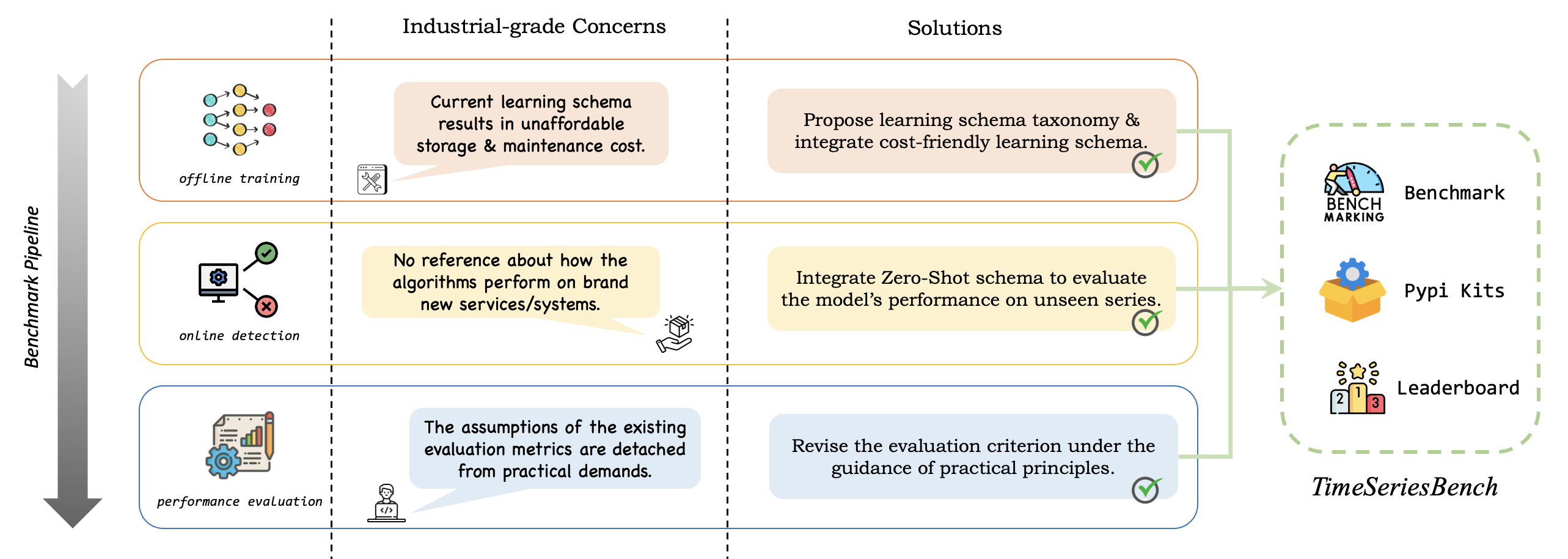
Figure 1. The industrial-grade concerns and TimeSeriesBench’s solutions on benchmarking univariate time series anomaly detection algorithms.

2. PRELIMINARIES

2.1. Time Series Anomaly Detection

A time series consists of successive observations of a metric (e.g., queries per second, sensor value, etc.) over a long period of time. The series can be represented as $T={x_{1},x_{2},\cdots,x_{n}}$, where $x_{i}$ represents an observation at timestamp $i$, and $n$ denotes the length of series. An anomaly within these time series data can be identified as a single point or a sequence of points that diverge significantly from their former customary patterns observed in the sequence. Anomaly detection methods project sequence observations into a probability distribution space to represent the degree of anomaly of the current observation, namely anomaly score, and compare it with a predefined threshold to determine whether an anomaly has occurred. Due to the scarcity of anomaly labels, existing deep-learning methods often opt for self-supervised training approaches.

2.2. Anomaly Types

Following the behavior-driven taxonomy (Lai et al., 2021), anomaly types can be roughly divided into point-wise outliers and pattern-wise outliers (Fig. 2). Point-wise outliers denote unexpected incidents like spikes or glitches on individual time points or within very short periods of time. Pattern-wise outliers represent anomalous subsequences that span over a certain period of time, often characterized as discordances or inconsistencies within the data.

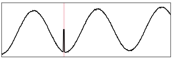
(a)

(b)

Figure 2. Illustrations of anomaly types. Anomalous segments are highlighted in pink.

3. TimeSeriesBench Settings

We launch TimeSeriesBench to integrate various aspects that are widely concerned into a pipeline to meet the diverse needs of scientific research and practical applications, and further promote the development of communities related to the field of time series anomaly detection. Aside from model implementation, the platform also takes some controversial issues, for instance, learning schema and evaluation criteria into consideration, to provide the researchers and engineers with a more comprehensive view of whether the models perform well in specific scenarios. In this section, we will illustrate the motivation and the implementation details of each inductive setting.

3.1. Datasets

High-quality datasets are the prerequisite for effective training and reasonable performance evaluations for models. Unfortunately, several publicly available time series datasets are claimed flawed due to their unrealistic anomaly density, or mislabeled ground truth (Wu and Keogh, 2021). Moreover, the proportion of different types of outliers can vary widely among datasets as the time series are gathered from irrelevant domains and applications. For example, Yahoo (Research, 2015) is dominated by global and contextual point-wise outliers on the basis of the behavior-driven taxonomy proposed by  (Lai et al., 2021) (the trivial first-order difference can achieve a comparable performance), while pattern-wise outlier plays a significant role in UCR archive (Wu, 2022a) (shown in Sec. 4). To this end, we gather multiple well-labeled real-world datasets covering many application domains to diversify the distributions of anomalies, meanwhile excluding markedly flawed datasets (some cases in  (Wu and Keogh, 2021)). Furthermore, we introduce a synthetic dataset generated from TODS (Lai et al., 2021) for the convenience of specific case analysis due to its good interpretability, because the time series adheres to well-designed distributions.

Real-world datasets. We employ AIOPS (Competition, 2018), WSD (Zhang et al., 2022a), Yahoo (Research, 2015), NAB (Ahmad et al., 2017b), and UCR (Wu, 2022a) for evaluations. Real-world datasets are more susceptible to uncertainties and tend to mix up with even inexplicable noise, which raises the demand in terms of model robustness. As the classes of anomalies are imbalanced among these datasets, practitioners focusing on the general-purpose model should refer to detection performance on all datasets, while application-oriented tasks need to pay more attention to performance on datasets that are strikingly similar to specific scenes. Meanwhile, we release a new dataset collected from the production environment, called NEK (Network Equipment KPI), for a more comprehensive evaluation.

Synthetic dataset. TODS (Lai et al., 2021) introduces a novel taxonomy, categorizes anomalies into five types, and publishes an anomaly generation toolkit in line with their claims. We conduct modifications based on their codes to generate longer and non-trivial anomalies, which would allow researchers to determine if models are capable of particular types of anomalies in a straightforward manner.

3.2. Learning Schema

Existing benchmarks take it for granted that the training process of the detector should comply with the naive task-specific schema, more specifically, training an exclusive detector for each time series solely leveraging its own historical patterns. We claim that it’s time to break the prevailing stereotype, especially for deep learning models, given the great transformations observed in application scenarios during recent years. On the one hand, with the maturation and improvement of surveillance systems in various fields, the quantity of time series to be monitored has experienced a substantial increase, reaching several orders of magnitude higher than before. This significantly raised the storage overheads if detectors are exclusive. On the other hand, the previous years witnessed many seminal works pertinent to foundational models for time series forecasting or other general tempo tasks (Anonymous, 2024b, c; Garza and Mergenthaler-Canseco, 2023; Zhou et al., 2023). We aspire to establish a foundation for the standardized training and evaluation of large-scale, general-purpose time series models, especially those designed for anomaly detection. Thus we introduce two novel learning schemas, called all-in-one mode and zero-shot mode, to assess the performance variations of models in scenarios involving large-scale data or zero-shot settings.

Naive schema. In this mode, we input a single time series for model training/fitting, and the trained detector is specifically employed for online detection on that particular series. Intuitively, this facilitates the model to make a more precise description of the temporal pattern given enough data. Nevertheless, it is worth noting that the volume of a single series tends to be insufficient.

All-in-one schema. In this mode, only one unified model instance is trained using all the sequences in the dataset, and the trained model is then applied for real-time anomaly detection across all sequences within the dataset. This schema exposes more patterns embedded in various series to the model, thereby providing an additional opportunity for the model to learn common and inherent traits shared among the time series. However, due to the differing definitions of anomalies across series, this carries the risk of confounding the model with conflicting information when detecting anomalies online (i.e., an anomaly present in a specific curve may not necessarily be considered an anomaly in other curves). Several novel methods (Zhang et al., 2022b; Ren et al., 2019) have adopted this schema driven by practical needs.

Zero-shot schema. In zero-shot mode, the whole dataset is split into two disjoint subsets. One subset is employed for model training and the other is used to evaluate the detection performance. This schema has been devised in light of practical considerations. Specifically, it addresses situations where a system is newly deployed with no prior historical data and a robust and adaptable model is required to navigate through this gap. This places higher demands on the model’s ability to capture the intrinsic representations of time series.

(a)

(b)

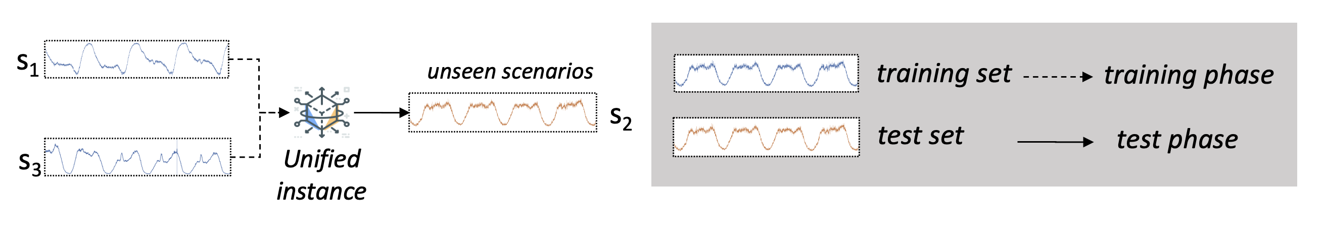
(c)

Figure 3. Illustrations of three learning schemas. $s_{n}$ indicates the n-th time series in the dataset.

3.3. Evaluation Criteria

A flawless evaluation criteria serves as the foundation for not only assessing the effectiveness of methods but also guiding model parameters optimization. Nevertheless, recent research has uncovered substantial limitations in commonly employed evaluation criteria, on which some seemingly absurd methods (e.g. noise generated by Random Guess) can outperform all others (Doshi et al., 2022; Sehili and Zhang, 2023; Kim et al., 2022; Garg et al., 2021). Also, some assumptions employed by certain evaluation criteria also conflict with the principles of industrial practice. Therefore, it is imperative to revise an anti-cheating and industrial-oriented evaluation protocol for our benchmark. It is crucial to emphasize that the selection of protocol is closely tied to the specific application context and determines how models perform with regard to the aspect you are interested in. In this paper, we focus on a generic real-time anomaly detection task.

In general, evaluation criteria employed in existing benchmarks can be roughly categorized into point-based protocols and range-based protocols. Point-based protocols like traditional F1 treat each individual data point as a separate sample, disregarding the holistic characteristics of the anomaly segment. Range-based protocols incorporate segment-level features, for instance, the detection latency (Jacob et al., 2020), into the evaluation.

In comparison to the aforementioned criteria, we prefer a protocol that aligns better with the typical workflow of real-time anomaly detection systems deployed in real-world scenarios. In practical application scenarios, whenever the anomaly score exceeds a predefined threshold, the system triggers an alert to notify the operators. Therefore, an operator tends to prioritize the following key issues:

• If a method can always detect anomalies within the anomaly segments, even if the anomaly score surpasses the threshold only once in each segment, it is still considered to possess a significant recall capability.

• Excessive false alarms would be rather frustrating for operators as they are obligated to examine each alert.

• The anomaly that lasts longer is likely to be more severe or challenging than the shorter ones.

• Detecting and addressing anomalies as early as possible can significantly mitigate the economic losses caused by abnormal situations.

To address issue a, we utilize a strategy of ”adjusting” the output of the algorithm, namely point-adjustment (PA), which is widely adopted (Qin et al., 2023; Shen et al., 2020; Su et al., 2019; Audibert et al., 2020; Li et al., 2021; Zhang et al., 2022b; Si et al., 2023). Under this strategy, all timestamps within an anomalous segment are assigned the highest anomaly score present within that segment, thus the whole anomaly segment is considered to be detected if at least one anomaly score surpasses the threshold. Then the F1 score is obtained in a point-based manner (point-wise PA in Fig. 4).

However, point-wise PA introduces biased true positives and false negatives due to the point-based criteria. As shown in Fig. 4, as a long anomaly segment is detected under point-adjustment, even if two false alarms are triggered, the Precision is up to 0.8, which contradicts the demand corresponding to issue b. The intrinsic flaw of this criteria is that the detection is rewarded generously while pulsing false alarm is penalized just once (Doshi et al., 2022). Garg et al. (Garg et al., 2021) revise the primitive PA from an event perspective. Each anomaly segment is treated as an individual event and contributes to a true positive or false negative only once. This protocol, namely event-wise PA, prevents the inflated evaluation scores originated from illogical criteria, while absolutely overlooking the length of the anomaly segments. Based on the observation c , we apply a severity coefficient $\ln{(k+e)}$ to adjust the true positive and false positive measurements associated with the given anomalous segment of length $k$. The protocol is called reduced-length PA, and we categorize it along with event-wise PA as event-based evaluation criteria.

Figure 4. Illustrations of evaluation protocols based on point-adjustment (PA). Point-wise PA gives an inflated score when some anomaly segments persist for a long duration. Event-wise PA treats each anomaly segment as an event, completely disregarding the length of the anomaly segment. Reduced-length PA considers the trade-offs between the two methods, holding greater practical significance in real-world applications.

Issue d demands exceptionally high data set quality, whereas some datasets fail to offer labels without positional bias. Due to the limitations of labels, we present this portion as supplementary content. More details can be found in Appendix A.

Besides, most statistical and deep learning methods generate anomaly scores under prediction-based or reconstruction-based frameworks, both heavily relying on the pattern provided by previous time windows. Hence, the recently concluded anomaly segment, particularly those with longer durations, has the potential to heavily interfere with the subsequent detection process. As shown in Fig. 5, from a qualitative perspective, we observe that the method accurately detects the frequency anomaly event. However, some unexpected false positives emerge due to the aforementioned reasons, resulting in an underestimated evaluation. We slightly extended the anomaly segments (less than 10 time points) to tolerate such occurrences, to make the evaluation more in line with our intuitive comprehension. We carefully handle edge cases to avoid merging two anomaly segments during the operation.

(a)

(b)

Figure 5. Illustrations of prolonging the anomaly segments. The blue line denotes the anomaly scores provided by a particular method. Considering the interference caused by anomalies on the detection of normal values, we should exclude false positives that occur immediately after an anomaly segment.

3.4. Algorithms

We adopt 17 semi-supervised/unsupervised methods that have raised significant discussion and wide-ranging impact in the field of univariate time series anomaly detection. The algorithms and implementation details are listed in Appendix B.5. From the perspective of method attributes, these methods can be divided into statistical methods and deep learning methods.

Statistical methods. These methods, including Sub-LOF (Breunig et al., 2000), SAND (Boniol et al., 2021), and MatrixProfile (Zhu et al., 2018), directly compute the minimum similarity between the current and the historical time window. This manner, however, would make the model highly sensitive to the data characteristics in specific scenarios, resulting in a lack of generalizability.

Deep learning methods. These methods learn the traits of normal patterns from past data in the training phase and judge whether the current metric is within the normal range in the online detection phase. Furthermore, deep learning methods can be categorized into the following families:

Prediction-based. These methods aim to predict the ”normal” value of the current metric according to the adjacent observations. If the ground truth is far from the predicted value, an anomaly alarm will be triggered.

Reconstruction-based. These methods aim to denoise the anomaly points by the encoding-decoding phase. If the reconstructed value is far from the ground truth, it can be assumed that an anomaly occurs.

VAE-based. These methods believe that the distribution mapping and sampling process can enhance the denoising effect of the model and learn a more robust representation of normal patterns.

General Time Series Model. The designed universal model structure in this class can be used for all time series tasks including time series forecasting, classification, and anomaly detection. They tend to introduce a more general inductive bias that aims to better represent the general features of time series.

(a)

(b)

(c)

Figure 6. Overall performance ranking using different learning schema under reduced-length $F1_{best}$. Methods are ranked in descending order according to the average of all scores. The row names denote the names of methods, while the column names denote the names of the datasets. The best score of each column is underlined. Due to the inherent assumptions behind the statistical methods being incompatible with the all-in-one and zero-shot schemas, these methods are not included in the ranking, and the related score cells are set to grey without values.

4. Experimental Results

In this section we conduct a rigorous analysis of the model’s effectiveness under various settings, aiming to provide meaningful research insights (RI) from unprecedented perspectives that can have implications for the design and application of methods. We aim to provide insights into the following research questions:

• How is the overall performance of the models, and what factors contribute to these results?

• How does the model’s performance vary under different learning schemas?

• How does the model’s performance vary in detecting different types of anomalies?

4.1. Overall Performance

The overall ranking list is presented in Fig. 6, including the performance of each method using naive, all-in-one, and zero-shot schema, respectively. Since statistical methods, especially those based on streaming, heavily rely on the premise of data being identically distributed, these methods are not well-suited for the all-in-one and zero-shot learning schemas. Therefore, we only evaluate them under the naive schema. First and foremost, (RI 1) The performance of various models under the naive and all-in-one learning schema can exhibit substantial disparities. It is thought-provoking that these differences do not show a clear bias, suggesting that these variations are the result of a combination of multifaceted factors, which is discussed in detail in Sec. 4.2. Additionally, (RI 2) given the consideration of errors arising from random dataset partitioning, the models demonstrated a relatively consistent performance across the all-in-one and zero-shot modes, as there may exist interdependence among time series in the same dataset.

(RI 3) Generally, the statistical methods exhibit great performance on the dataset with relatively stable shapelets and low noise level (UCR), but work poor on other datasets with more noise. For deep learning based models, contrary to our expectations, the overall performances of the models that contain more complicated structures are not satisfactory. According to our examination across existing datasets, a substantial portion of anomalies in real-world datasets exhibit noticeable deviations from their very close neighboring points (sudden spikes or drops), especially for AIOPS, WSD, and Yahoo. These anomalies can be categorized as either contextual outliers or global outliers, both of them belonging to point-wise anomaly type. Due to its ability to capture very local temporal correlations and its ease of convergence, AR surpasses a number of modern networks in cases where point-wise anomalies dominate. We present a case (Fig. 7) from the AIOPS dataset to vividly demonstrate this phenomenon. Even though these point-wise anomalies seem to be quite evident, a significant portion of the methods are unable to handle such events effectively, most likely because they are highly sensitive to noise and may struggle to generalize well. More cases are listed in Appendix D. As numerous factors can lead to a decrease in performance for DNNs, (RI 4) we summarize the major factors that result in the underperformance of some deep learning methods in point-wise anomaly detection tasks:

High noise level. As shown in the former case, the noise can introduce additional variability and random fluctuations in the data, making it harder for the model to distinguish between genuine anomalies and noise-induced fluctuations.

Lack of training data. Models with complicated structures usually require a larger volume of training data to avoid overfitting due to their higher degrees of freedom and flexibility. Similarly, models that employ intricate loss functions often necessitate a greater amount of training data, including diverse examples, to prevent the emergence of falling into local minima and even trivial solutions.

Trends with large periods. Some data may exhibit long-term trends or patterns that span large periods. These trend components can cause the data distribution to deviate from the comfort zone of the model, causing the model to calculate anomaly scores based on a biased data distribution it has never encountered before.

Unreasonable inductive bias. Deep learning models rely on their architectural design and optimization algorithms to detect anomalies in a semi-supervised manner. If the chosen model architecture or optimization approach is not well-suited for point-wise anomaly detection, the models may have an unreasonable inductive bias that hampers their ability to accurately detect anomalies.

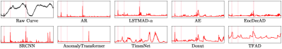
Figure 7. Illustrations that some methods fail to effectively detect point-wise anomalies in certain scenarios. The black line represents the original curve, while the red line represents the anomaly scores provided by the method. Anomalous segments are highlighted in pink.

To demonstrate the impact of (RI 4) in a more impressive manner, we conduct an intriguing experiment under the all-in-one learning schema, where the training data is abundant and diverse. In this experiment, we apply first-order differencing to all the training data before feeding it into the model for training. Subsequently, we evaluate the model’s performance on the same first-order differenced dataset. Despite the potential increase in noise level caused by first-order differencing on the original data, it significantly magnify point-wise anomalies while alleviating the effect brought by the continuous and consistent trend factor, as is vividly shown in Fig. 8. Benefiting from this, some methods can achieve a performance improvement of more than 30% on this dataset after the differencing process. It is important to note that we do not recommend relying solely on differenced data for anomaly detection. Differencing can make the temporal pattern information more ambiguous and noisy, significantly reducing the model’s ability to detect pattern-wise anomalies and thus lowering the detection ceiling. More importantly, it is imperative for newly proposed methods to place greater emphasis on these factors to avoid poor results on these distinct point-wise anomalies.

Figure 8. Illustrations that first-order differencing can amplify the degree of outlierness of point-wise anomalies while introducing noise with higher variance.

4.2. Performance in Fine-Grained Scenarios

Merely referring to aggregated data at the granularity of datasets is insufficient to gain a profound understanding of the model’s performance. We carry out a fine-grained comparison of model performance from the perspectives of both learning schema and anomaly type. The UCR dataset is widely acknowledged for its comprehensive annotation of various anomaly types, making it a well-labeled dataset. Additionally, each time series in the UCR dataset is guaranteed to contain only one anomaly, which facilitates the categorization of different anomaly types. To further refine our analysis, we partition the UCR dataset into two subsets based on its supplemental materials (Wu, 2022b): one subset exclusively consisting of point-wise anomalies and another subset focusing solely on pattern-wise anomalies. We form a 2x2 matrix to reflect the variations in model performance under different conditions by incorporating the dimensions of ”naive” and ”all-in-one” learning schemas, along with different types of anomalies, as shown in Fig. 9.

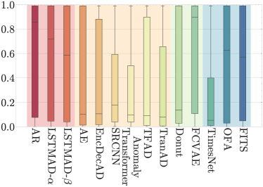
(a)

(b)

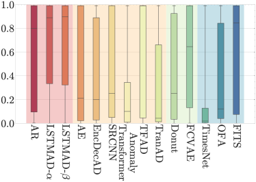
(c)

(d)

Figure 9. The 2x2 matrix reflecting the variations in model performance under different conditions. We denote prediction, reconstruction, VAE-based, and general time series methods in light red, yellow, green, and blue backgrounds.

From the boxplots, (RI 5) no solution can always outperform the others in all situations. It is also apparent that (RI 6) the majority of models exhibit a significantly higher detection performance for point-wise anomalies compared to pattern-wise anomalies regardless of the learning schema employed. On a more detailed level, (RI 7) prediction-based models excel in identifying point-wise anomalies, as the steep peak/valley is unpredictable in most cases. Due to the inclusion of a more diverse data distribution under all-in-one learning schema, the models are more likely to learn robust representations of patterns. (RI 8) As a result, under the all-in-one learning schema, there is a significant improvement in the detection performance of point-wise anomalies. This observation is particularly pronounced in the case of the Yahoo dataset each time series of which is relatively short. With regard to pattern-wise anomalies which are considered to be more challenging, the situation becomes more complex and interesting. (RI 9) Methods that aim to generate the temporal window after projecting them to low-dimensional representations (Donut and FCVAE) surpass all others in detecting pattern-wise anomalies, while the performance greatly declines when under the all-in-one mode. The former indicates that the assumption of low-dimensional representations hardly reconstructing high-level pattern-wise anomaly indeed works. An illustration is presented to confirm this in Fig. 10(a), where Donut can easily handle the ”smooth” high-level anomaly. However, the performance deteriorates or even becomes ineffective under the all-in-one mode (Fig. 10(b)). We hypothesize that the capacity of low-rank representations may struggle to cover the diverse data distributions present in various curves. Also, (RI 10) although the general time series methods (TimesNet, OFA, FITS) perform well in other time series tasks, they struggle to outperform methods specifically designed for anomaly detection tasks. This may indicate that there is a gap between time series anomaly detection tasks and general time representation tasks. For example, anomaly detection tasks may require models to have a stronger denoising effect. These gaps need special attention when designing models for anomaly detection tasks.

(a)

(b)

Figure 10. Case study on CIMIS44AirTemperature2 which contains an easily understandable pattern-wise anomaly.

4.3. Trade-off Between Performance, Cost, and Efficiency

When deploying algorithms in real-world scenarios, it is often necessary to strike a balance between performance, storage costs, and inference speed. Notably different from other surveys, in this benchmark, we prefer inference time over training time due to the practical needs of anomaly detection. Each factor plays a critical role in determining the feasibility and practicality of the deployed algorithm. The trade-offs between these considerations are important to ensure an efficient and effective deployment that meets the specific requirements and constraints of the application. For example, real-time monitoring or critical systems may prioritize efficiency to detect anomalies promptly and respond quickly, while IoT (Internet of Things) devices with limited on-chip memory have to focus on the performance of models with a small number of parameters. We exclude the statistical methods, as their inference time is not a fixed value (polynomially correlated with the volume of historical data). Also, We exclude TFAD because it does not align with the real-time manner. As shown in Fig. 11, the inference time for a single sample is far less than 50 milliseconds for all methods under our experimental platform. The learning-based AR exhibits the most favorable gain-to-cost ratio among all methods. FCVAE takes the longest time to inference due to its multi-epoch MCMC process. EncDecAD has the second longest inference time because it utilizes LSTM to perform inference for 100 time steps. (RI 11) In addition to providing guidance for practical applications, we aim for this perspective and toolkit to assist in discovering the scaling law in the field of time series anomaly detection under more reasonable inductive bias and larger parameter spaces.

Figure 11. The triad of the model’s performance, cost, and efficiency trade-off. The x-axis represents the total inference time (batch size set to 1) of the detectors on AIOPS_7103fa0f-cac4-314f-addc-866190247439 (around 140,000 samples) under default parameters. The y-axis represents the average performance of the models on all datasets under the all-in-one learning schema. The size of the scatter points denotes each method’s cube root of the number of parameters.

5. Conclusion AND FUTURE DIRECTIONS

In this paper, we propose TimeSeriesBench, a comprehensive and application-oriented benchmark for evaluating the performance of existing and emerging UTS anomaly detection methods. TimeSeriesBench takes into account existing industrial concerns and conducts a comprehensive performance evaluation of some well-known and latest methods under settings that meet industrial requirements. Also, it offers unprecedented perspectives for measuring algorithm performance, meanwhile laying a solid foundation for the development of Foundation Models in the field. Moreover, TimeSeriesBench includes a user-friendly toolkit and leaderboard, offering easy-to-use interfaces that allow researchers and practitioners to focus on advancing their algorithms without getting entangled in repetitive tasks. We intend to incorporate more latest methods/evaluation protocols and employ more high-quality data. Also, we will continue to monitor the latest developments in general foundation models for time series within the realm of anomaly detection, adapting them accordingly within our benchmark. Additionally, whether you propose deep learning or statistical methods, we welcome your participation in our leaderboard to help drive the development of the time series anomaly detection community.

Appendix A Delay Constraint

We cope with the issue c (in Sec. 3.3) by imposing strict constraints on the detection latency. As depicted in the illustration (Fig. 12), assuming the latency limit ($k$) is set to 3, an anomaly is considered effectively detected only if it is identified within three sampling points after its occurrence. We designate this strategy as k-delay adjustment. This measure enables a more precise assessment of whether the model can meet the requirement of the scenario where there is a high demand for real-time responsiveness. It is equally essential to acknowledge that this approach is applicable only to datasets whose anomalies are labeled without positional bias. We conduct experiments on the selected datasets with non-biased labels. The overall results in shown in Table 2.

Figure 12. Illustrations of k-delay adjustment. This strategy can be combined with point-adjustment as a complementary evaluation paradigm.

Appendix B Details about Experimental settings

B.1. Experimental Platform

All experiments are performed on a server equipped with Dual Intel(R) Xeon(R) Silver 4316 (12-core) and 256GB RAM. The operating system of this server is Ubuntu 22.04 LTS. An NVIDIA GeForce RTX 3090 24GB GDDR6 GPU is utilized to accelerate the training and inference processes of all models.

B.2. Datasets

With the exception of the UCR dataset and AIOPS dataset where the training and testing sets are already specified, we partition each time series into training, validation, and test sets following a 4:1:5 ratio. Given that anomalies in some datasets are randomly distributed, the test set of some sequences does not contain any anomalies after partitioning. Therefore, we exclude these anomaly-free sequences from consideration. Due to the fact that the original implementation of TODS sometimes generates anomalies that do not match their specified anomaly types (e.g., constructing trend and seasonal anomalies may result in obvious global outliers), we modify the anomaly generation code in TODS to ensure that the injected anomalies align more closely with their defined types. It is worth noting that we aggregate the overall evaluation at the dataset level instead of the curve level because the imbalance in sample sizes across different datasets can lead to biased results.

B.3. Learning Schema

We evaluated existing methods under all proposed learning schemas to obtain a more comprehensive understanding of the model’s performance from different perspectives. Statistical methods are not assessed under all-in-one and zero-shot schema due to assumption conflict. Under the all-in-one schema, taking the UCR dataset as an example, we mix all samples together from all time series’ training sets during the training phase. Under zero-shot schema, we use a fixed random seed to split UCR into two subsets, each of which includes half of the time series. We mix all training samples from one subset, and the other acts as the test set. All methods share the same training set in zero-shot mode.

B.4. Evaluation Metrics

Following the event-based evaluation criterion outlined in Sec. 3.3, we establish two concrete metrics, namely $F1_{best}$ and $AUPRC$. $F1_{best}$ denotes the highest F1 score calculated under reduced-length point-adjustment when iterating over all possible thresholds. $AUPRC$ calculates the area under the precision-recall curve generated according to reduced-length point-adjustment, which is widely applied in cases where class imbalance is present in the data. While $F1_{best}$ can measure the best detection performance that the model can achieve on the current test set, $AUPRC$ provides a more nuanced evaluation of the model’s performance across different levels of recall, which can be important in anomaly detection. A model with a higher $AUPRC$ tends to be more robust.

B.5. Details of Algorithms

B.5.1. Descriptions of Algorithms

Here is the publication date and detailed introduction of all baselines. We will continuously incorporate new methods, and if you are willing to integrate your approach into our benchmark, please feel free to initiate a pull request on GitHub or send us an email.

MatrixProfile (2018) (Zhu et al., 2018). MatrixProfile is a data structure with corresponding algorithms that can measure the minimum distance between the current and the historical time series subsequence, and detect if there is an anomaly according to the measurement.

SAND (2021) (Boniol et al., 2021). SAND leverages the K-shape (Paparrizos and Gravano, 2016) to cluster normal patterns and compares the upcoming time series subsequence with the cluster centroid in a streaming manner.

Sub-LOF (2000) (Breunig et al., 2000). Sub-LOF is an unsupervised learning algorithm that identifies outliers by measuring the local deviation of a given data point with respect to its neighbors.

AR (2005) (Rousseeuw and Leroy, 2005). AutoRegression (AR) holds the assumption that there exists a linear dependence between each individual instance and its past observations. We implement the model using a linear layer in Pytorch and apply first-order differencing on all the data to eliminate potential trend components as the AR model requires time series data to be stationary.

LSTMAD (2015) (Malhotra et al., 2015). LSTMAD employs Long Short-Term Memory (LSTM) networks to capture the temporal dependency among the time windows. As the paper does not provide a detailed description of the algorithm and there is no official source code available, we implement LSTMAD in two forms: LSTMAD-$\alpha$ in a seq2seq manner and LSTMAD-$\beta$ in a multi-step prediction manner.

AE (2011) (Ng et al., 2011). AutoEncoder (AE) projects a time window that ends at the current timestamp to the lower-dimensional latent space and subsequently reconstructs the window. The reconstructed value of the last timestamp is compared with the ground truth value to calculate the anomaly score.

EncDecAD (2016) (Malhotra et al., 2016). EncDecAD additionally introduces LSTM to AE to obtain more complicated representations.

Donut (2018) (Xu et al., 2018). Donut utilizes variational autoencoder and modified ELBO loss to denoise the anomalies and further learn the robust representation of normal patterns.

FCVAE (2024) (Wang et al., 2024). Frequency-enhanced Conditional Variational Autoencoder (FCVAE) incorporates both global and local frequency characteristics into the conditioning of the CVAE framework, greatly improving the accuracy of reconstructing the normal data.

SRCNN (2019) (Ren et al., 2019). SRCNN borrows the technique of visual saliency detection, combining Spectral Residual (SR) and Convolutional Neural Network (CNN) together to detect time series anomalies.

AnomalyTransformer (2022) (Xu et al., 2022). AnomalyTransformer utilizes an attention mechanism to compute the association discrepancy.

TFAD (2022) (Zhang et al., 2022b). TFAD exploits the information in both time and frequency domains to amplify the traits while creating various data augmentation methods to overcome the lack of anomaly data.

TranAD (2022) (Tuli et al., 2022). TranAD incorporates the principles of adversarial learning to develop a training framework with two stages while integrating the strengths of self-attention encoders to capture the temporal dependency embedded in the time series.

TimesNet (2023) (Wu et al., 2023). TimesNet is a general time series model that is capable of handling multiple tasks such as time series forecasting, anomaly detection, and classification. It folds the time series to 2-D space according to frequency information and uses a vision backbone to capture the 2-D dependencies within the reshaped time series.

OFA (2023) (Tian Zhou, 2023). One-Fits-All (OFA) finetunes the pre-trained GPT backbone on time series data to address the issue of lacking a large amount of data for training.

FITS (2024) (Anonymous, 2024a). FITS employs only a single layer frequency domain linear transformation to model the general temporal dependencies and achieves commendable results on general time series tasks with a minimal number of training parameters.

B.5.2. Implementation details of Algorithms

All methods are implemented in Sklearn or Pytorch, either based on open-source repositories or reproduced based on the original paper’s description. All methods are integrated into the TimeSeriesBench suite. If the model has specific hyperparameters set for a particular dataset, we use the parameters specified for that dataset. Otherwise, we use the default hyperparameters provided in the source code. The early stopping mechanism is applied to all methods on the validation set.

Appendix C TimeSeriesBench Toolkit

One of our primary intentions is to develop a suite that liberates practitioners from burdensome workflows, allowing them to engage in TSAD tasks with greater ease and efficiency. Existing suites narrowly offer convenience for the implementation of new methods with primitive workflows and rudimentary evaluations. Here, benefiting from the modular architecture of TimeSeriesBench, we provide a diverse range of extension interfaces implemented in Python to enable the community to conduct comparative experiments more flexibly and effortlessly, meanwhile reserving the possibilities for innovative and exceptionally demanding experiments, which might unlock unexplored avenues of research.

The overview of the toolkit is shown in Fig. 13. The dataset interface and algorithm interfaces are provided to allow evaluations on new or private datasets and novel methods under all learning schemas. All plots of raw curves and scores are saved for specific investigation. Previously mentioned flaws in evaluation criteria have sparked a research fervor and several latest works are dedicated to providing evaluation protocols according to different assumptions (Kim et al., 2022; Wagner et al., 2023; Huet et al., 2022; Paparrizos et al., 2022a; Doshi et al., 2022; Scharwächter and Müller, 2020). Thus we also expose an interface for swiftly developing neo-criteria for evaluation grounded in realistic assumptions and evaluating the performance of all methods w.r.t various datasets. In some scenarios, there might be a trade-off between model accuracy and model training/testing cost. Therefore, we also provide a runtime statistics interface to conveniently track and analyze the runtime information of the model.

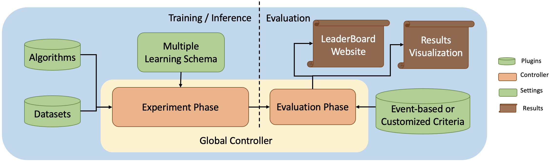
Figure 13. Overview of TimeSeriesBench Toolkit.

We provide four kinds of workflows to meet different research needs for time series anomaly detection: algorithms benchmarking, algorithm development, evaluation criteria development, and performance analysis. The following are typical audiences for TimeSeriesBench toolkit:

• Algorithm Researches. TimeSeriesBench offers a flexible interface for implementing, training, and testing new algorithms. Researchers can choose all the mentioned schemas for model training and testing. The framework also provides a full pipeline for loading datasets, running experiments, conducting evaluations, and performing analysis such as generating plots and comparing anomaly scores.

• Evaluation Researchers. TimeSeriesBench offers a flexible interface for implementing evaluation protocols based on anomaly scores and ground truth labels. Researchers can easily evaluate existing methods according to their specific protocols. The framework also allows evaluation based on offline scores of methods generated by merely once training and test phase.

• Practitioners of Community or Enterprise. TimeSeriesBench provides a unified and clear dataset format, making it easy to introduce private datasets. It also allows for easy performance comparison of baselines on custom datasets, providing overall performance in CSV format based on protocols suitable for specific applications. Moreover, TimeSeriesBench allows practitioners to record runtime statistics such as model parameter size and inference time, enabling trade-offs between performance, cost, and efficiency.

Compared to existing benchmark suites on univariate time series anomaly detection (Jacob et al., 2020; Lai et al., 2021; Paparrizos et al., 2022b; Wenig et al., 2022), our benchmark suite incorporates real-world scenarios and challenges, aiming to replicate the complexities and nuances encountered in practical applications. This enables researchers and practitioners to gain deeper insights into the strengths and weaknesses of various deep learning approaches, and is well-prepared for the emergence and development of Foundation Models (FMs) in the field of time series anomaly detection. For more information about TimeSeriesBench, please refer to our project and the website of the leaderboard.

Table 1. Comparison among TimeSeriesBench and existing UTS anomaly detection benchmark suites. TimeSeriesBench presents more angles for performance evaluation, meanwhile offering user-friendly interfaces for up-to-date model and evaluation protocol developments.

Suites		Exathlon(Jacob et al., 2020)	TODS(Lai et al., 2021)	TSB(Paparrizos et al., 2022b)	TimeEval(Wenig et al., 2022)	Ours
Data Source	Real-World	✓	✓	✓	✓	✓
	Synthetic	✗	✓	✓	✓	✓
Learning Schema	one-by-one	✓	✓	✓	✓	✓
	all-in-one	✗	✗	✗	✗	✓
	zero-shot	✗	✗	✗	✗	✓
Supported Eval-Criteria	point-based	✓	✓	✓	✓	✓
	range-based	✓	✗	✓	✓	✓
	event-based	✗	✗	✗	✗	✓
Extensibility	Dataset	✗	✓	✓	✓	✓
	Method	✓	✓	✗	✓	✓
	Eval-Criteria	✗	✗	✗	✓	✓
	RT statistics	✗	✗	✗	✗	✓

Appendix D Informative Cases on Point-wise Anomalies

Other cases are presented below to demonstrate how the lack of training data (Fig. 14) or trends (Fig. 15) with large periods induce poor performance for point-wise anomalies. Some methods are unable to yield meaningful results on most time series, which may result from their unreasonable inductive bias.

(a)

(b)

Figure 14. Case study on Yahoo_A3Benchmark-TS13 shows that lack of training data induces poor performance.

Figure 15. Case study on Yahoo_A3Benchmark-TS14 shows that trends with large periods induce poor performance. The scores are obtained under the all-in-one learning schema, eliminating the impact of insufficient data.

Appendix E Supplementary statistics

E.1. Overall Performance

Detailed experimental results under all learning schemas are listed in Table 3,  4,  5. Best scores are highlighted in bold, and second-best scores are highlighted in bold and underlined. Due to the inherent assumptions behind the statistical methods being incompatible with the all-in-one and zero-shot schemas, the related scores are set to ”-”.

E.2. Impacts of Different Evaluation Criteria

We also provide the evaluation results under point-wise PA (Point Adjustment), reduced-length PA, and event-wise PA respectively (Table 6,  7,  8). Point-wise PA often results in inflated scores, while event-wise PA completely neglects the length of the anomaly segments. Best scores are highlighted in bold, and second-best scores are highlighted in bold and underlined. Due to the inherent assumptions behind the statistical methods being incompatible with the all-in-one and zero-shot schemas, the related score are set to ”-”.

E.3. Impacts of Different Learning Schemas

Table  9 shows the performance differences on all datasets using different learning schemas. Best scores are highlighted in bold, and second-best scores are highlighted in bold and underlined. Performance improvements exceeding 5% are marked with $\uparrow$, while performance declines exceeding 5% are marked with $\downarrow$.

E.4. Performance, Cost, Efficiency Trade-off

The model’s performance, cost, and efficiency trade-off under naive and zero-shot learning schema are shown in Fig. 16 and Fig. 17.

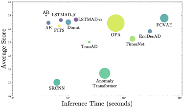
Figure 16. The triad of the model’s performance, cost, and efficiency trade-off. The y-axis represents the average performance of the models on all datasets under the naive learning schema. The size of the scatter points denotes each method’s cube root of the number of parameters.

Figure 17. The triad of the model’s performance, cost, and efficiency trade-off. The y-axis represents the average performance of the models on all datasets under the zero-shot learning schema. The size of the scatter points denotes each method’s cube root of the number of parameters.

Table 2. Performance comparison using all-in-one learning schema under K-delay reduced-length $F1_{best}$ and $AUPRC$

Method	AIOPS (K=10)		NAB (K=150)		TODS (K=3)		WSD (K=10)		Yahoo (K=3)		UCR (K=50)		NEK (K=10)
	$F1_{best}$	$AUPRC$	$F1_{best}$	$AUPRC$	$F1_{best}$	$AUPRC$	$F1_{best}$	$AUPRC$	$F1_{best}$	$AUPRC$	$F1_{best}$	$AUPRC$	$F1_{best}$	$AUPRC$
MatrixProfile	-	-	-	-	-	-	-	-	-	-	-	-	-	-
SAND	-	-	-	-	-	-	-	-	-	-	-	-	-	-
Sub-LOF	-	-	-	-	-	-	-	-	-	-	-	-	-	-
AR	0.7815	0.766	0.5334	0.407	0.6748	0.6827	0.7251	0.6888	0.9451	0.9345	0.3422	0.3121	0.9137	0.9154
LSTMAD-$\alpha$	0.7819	0.7924	0.4235	0.2928	0.6437	0.6424	0.7627	0.7276	0.7946	0.7767	0.4494	0.4063	0.9196	0.9308
LSTMAD-$\beta$	0.7826	0.7957	0.4275	0.2928	0.6234	0.63	0.7593	0.7248	0.8033	0.7841	0.4464	0.4073	0.9458	0.9561
AE	0.7077	0.71	0.3685	0.255	0.5843	0.5551	0.7522	0.719	0.8076	0.7882	0.2233	0.1881	0.9439	0.9513
EncDecAD	0.6744	0.6434	0.394	0.2602	0.5346	0.5328	0.6641	0.6271	0.5751	0.5277	0.2064	0.1723	0.9348	0.9256
Donut	0.5618	0.5262	0.4014	0.2859	0.6296	0.617	0.6317	0.5765	0.6423	0.6089	0.1869	0.1556	0.5618	0.4383
FCVAE	0.7389	0.7256	0.5991	0.4845	0.6281	0.6117	0.6838	0.6372	0.847	0.8242	0.3249	0.2813	0.7439	0.6557
SRCNN	0.6253	0.5748	0.3072	0.2383	0.1816	0.1069	0.6267	0.5744	0.1605	0.0978	0.2358	0.2019	0.5446	0.5189
AnomalyTransformer	0.306	0.1596	0.3655	0.2657	0.1331	0.0674	0.4326	0.2876	0.1751	0.0978	0.1243	0.0948	0.6075	0.4891
TFAD	0.4578	0.362	0.15	0.0849	0.4658	0.3988	0.6165	0.569	0.9281	0.9144	0.4206	0.4034	0.3133	0.1913
TranAD	0.6302	0.5726	0.4406	0.3254	0.4199	0.3944	0.588	0.5219	0.511	0.4551	0.1472	0.1261	0.8932	0.8696
TimesNet	0.4663	0.4199	0.433	0.3105	0.3792	0.3232	0.4063	0.3349	0.5242	0.4988	0.0704	0.0501	0.9028	0.9174
OFA	0.4689	0.3818	0.4145	0.2901	0.4664	0.4147	0.605	0.5593	0.7267	0.6979	0.1718	0.1371	0.7155	0.6536
FITS	0.6623	0.6474	0.4341	0.302	0.5232	0.5423	0.6848	0.6573	0.9013	0.8903	0.2802	0.2585	0.8335	0.8122

Table 3. Performance comparison using naive learning schema under reduced-length $F1_{best}$ and $AUPRC$.

Method	AIOPS		NAB		TODS		WSD		Yahoo		UCR		NEK
	$F1_{best}$	$AUPRC$	$F1_{best}$	$AUPRC$	$F1_{best}$	$AUPRC$	$F1_{best}$	$AUPRC$	$F1_{best}$	$AUPRC$	$F1_{best}$	$AUPRC$	$F1_{best}$	$AUPRC$
MatrixProfile	0.0281	0.0097	0.1769	0.0975	0.2058	0.1407	0.0371	0.0234	0.2051	0.1445	0.5066	0.4711	0.3163	0.2439
SAND	0.0674	0.0262	0.3036	0.2169	0.2544	0.1879	0.0952	0.0666	0.468	0.4343	0.5494	0.5344	0.1758	0.1304
Sub-LOF	0.3764	0.31	0.6982	0.5835	0.5791	0.5236	0.7194	0.6895	0.4875	0.4443	0.5806	0.5325	0.6807	0.6423
AR	0.7517	0.75	0.9035	0.8691	0.7472	0.7677	0.868	0.8609	0.9195	0.9057	0.4454	0.4026	0.9555	0.9647
LSTMAD-$\alpha$	0.8081	0.8236	0.8984	0.8358	0.7015	0.7201	0.9381	0.9298	0.5496	0.5026	0.4836	0.441	0.9971	0.9959
LSTMAD-$\beta$	0.8034	0.8219	0.9031	0.841	0.7589	0.7706	0.939	0.9309	0.5366	0.4868	0.4366	0.3931	0.9744	0.9716
AE	0.7222	0.7295	0.8751	0.8146	0.6842	0.6675	0.918	0.9049	0.612	0.5692	0.4198	0.3879	0.9801	0.9824
EncDecAD	0.7583	0.7621	0.8752	0.8136	0.6359	0.6234	0.9285	0.9214	0.5018	0.449	0.3178	0.2829	0.755	0.733
Donut	0.6957	0.6791	0.8397	0.7607	0.7207	0.7061	0.8787	0.8668	0.6813	0.6441	0.4409	0.3968	0.9885	0.9923
FCVAE	0.7851	0.8079	0.874	0.8539	0.7145	0.7162	0.9087	0.8966	0.6883	0.6498	0.5873	0.5482	0.8977	0.9128
SRCNN	0.1627	0.0972	0.5802	0.4946	0.3042	0.1931	0.1785	0.0993	0.1261	0.0662	0.3227	0.2667	0.4365	0.3501
AnomalyTransformer	0.3728	0.3053	0.7739	0.691	0.2827	0.182	0.2984	0.2128	0.145	0.0879	0.3104	0.2548	0.3997	0.2617
TFAD	0.3551	0.2529	0.5746	0.532	0.4526	0.3943	0.7561	0.7115	0.781	0.7501	0.3398	0.3077	0.625	0.5786
TranAD	0.6486	0.5798	0.9101	0.8627	0.2531	0.1988	0.6738	0.6089	0.562	0.516	0.2527	0.2199	0.9071	0.8928
TimesNet	0.6737	0.6674	0.8419	0.7845	0.3695	0.3327	0.8684	0.8466	0.4444	0.4089	0.2493	0.2142	0.9335	0.9388
OFA	0.6891	0.6973	0.8869	0.8468	0.6263	0.5683	0.8784	0.8683	0.7512	0.7145	0.4169	0.3804	0.9471	0.9553
FITS	0.7139	0.7187	0.8617	0.8168	0.5371	0.5119	0.8796	0.8822	0.7564	0.7235	0.4092	0.3657	0.8975	0.9032

Table 4. Performance comparison using all-in-one learning schema under reduced-length $F1_{best}$ and $AUPRC$.

Method	AIOPS		NAB		TODS		WSD		Yahoo		UCR		NEK
	$F1_{best}$	$AUPRC$	$F1_{best}$	$AUPRC$	$F1_{best}$	$AUPRC$	$F1_{best}$	$AUPRC$	$F1_{best}$	$AUPRC$	$F1_{best}$	$AUPRC$	$F1_{best}$	$AUPRC$
MatrixProfile	-	-	-	-	-	-	-	-	-	-	-	-	-	-
SAND	-	-	-	-	-	-	-	-	-	-	-	-	-	-
Sub-LOF	-	-	-	-	-	-	-	-	-	-	-	-	-	-
AR	0.8214	0.8203	0.8881	0.8462	0.7859	0.8365	0.9276	0.9179	0.948	0.9392	0.4636	0.4182	0.9612	0.9719
LSTMAD-$\alpha$	0.8141	0.8343	0.8492	0.7889	0.7538	0.7738	0.9467	0.9401	0.8	0.7829	0.6144	0.5598	0.9349	0.9528
LSTMAD-$\beta$	0.8151	0.8377	0.8484	0.7821	0.7495	0.7771	0.9445	0.9391	0.8114	0.7922	0.6101	0.5602	0.961	0.9781
AE	0.7448	0.7523	0.8375	0.7793	0.7712	0.7441	0.9192	0.9138	0.8205	0.8018	0.3644	0.3208	0.9609	0.9757
EncDecAD	0.7003	0.6894	0.8336	0.7786	0.6534	0.6592	0.8353	0.8182	0.5842	0.5378	0.3333	0.2867	0.9534	0.9538
Donut	0.5827	0.5578	0.7966	0.7085	0.836	0.8381	0.7666	0.7271	0.6498	0.6161	0.4	0.3395	0.5801	0.4923
FCVAE	0.7593	0.7521	0.8857	0.8587	0.8526	0.8535	0.8121	0.7814	0.8537	0.8292	0.4766	0.418	0.8148	0.793
SRCNN	0.6672	0.632	0.635	0.5648	0.2598	0.1658	0.7742	0.7337	0.1728	0.1056	0.3791	0.3176	0.6173	0.5906
AnomalyTransformer	0.3656	0.2103	0.7322	0.6432	0.2631	0.1561	0.5838	0.4227	0.2377	0.1468	0.2372	0.1777	0.666	0.5539
TFAD	0.4889	0.4062	0.4679	0.3996	0.5626	0.5411	0.8016	0.7602	0.9361	0.9236	0.4941	0.4646	0.4103	0.2853
TranAD	0.6561	0.6049	0.8567	0.7921	0.5624	0.5291	0.7409	0.6995	0.5211	0.4643	0.2483	0.2181	0.9571	0.9524
TimesNet	0.4988	0.4657	0.8544	0.8055	0.5032	0.4293	0.539	0.4602	0.5341	0.5098	0.1856	0.149	0.9257	0.9459
OFA	0.5544	0.4993	0.861	0.7911	0.6187	0.6129	0.8111	0.7877	0.766	0.7414	0.2888	0.2334	0.7642	0.7389
FITS	0.6986	0.6966	0.8683	0.8196	0.7146	0.7446	0.8788	0.8745	0.9261	0.9189	0.428	0.391	0.9625	0.9719

Table 5. Performance comparison using zero-shot learning schema under reduced-length $F1_{best}$ and $AUPRC$.

Method	AIOPS		NAB		TODS		WSD		Yahoo		UCR		NEK
	$F1_{best}$	$AUPRC$	$F1_{best}$	$AUPRC$	$F1_{best}$	$AUPRC$	$F1_{best}$	$AUPRC$	$F1_{best}$	$AUPRC$	$F1_{best}$	$AUPRC$	$F1_{best}$	$AUPRC$
MatrixProfile	-	-	-	-	-	-	-	-	-	-	-	-	-	-
SAND	-	-	-	-	-	-	-	-	-	-	-	-	-	-
Sub-LOF	-	-	-	-	-	-	-	-	-	-	-	-	-	-
AR	0.8013	0.7928	0.8967	0.8306	0.7975	0.8589	0.926	0.9066	0.9366	0.9234	0.487	0.443	0.9641	0.9723
LSTMAD-$\alpha$	0.8184	0.8304	0.8593	0.7913	0.677	0.6834	0.9349	0.92	0.8277	0.8141	0.5927	0.539	0.9539	0.9692
LSTMAD-$\beta$	0.8073	0.8233	0.8556	0.7915	0.593	0.5935	0.9357	0.9219	0.7942	0.7745	0.5603	0.5128	0.9613	0.9718
AE	0.7689	0.7787	0.8538	0.7917	0.7105	0.6926	0.8969	0.8841	0.8595	0.8437	0.3239	0.284	0.9591	0.9727
EncDecAD	0.7537	0.7694	0.85	0.7796	0.7089	0.6829	0.8306	0.8163	0.5958	0.5499	0.3209	0.2764	0.9441	0.9526
Donut	0.6863	0.6724	0.7187	0.603	0.6223	0.5933	0.7934	0.7568	0.7034	0.6733	0.4148	0.367	0.6204	0.5069
FCVAE	0.7983	0.8143	0.9385	0.8895	0.7987	0.7884	0.7707	0.7316	0.796	0.7683	0.4101	0.3642	0.7979	0.8044
SRCNN	0.6888	0.6507	0.6421	0.6205	0.2977	0.18	0.7414	0.6936	0.1437	0.0859	0.3582	0.2889	0.5261	0.4788
AnomalyTransformer	0.4361	0.2757	0.5601	0.4912	0.2199	0.1531	0.3027	0.2065	0.4302	0.3613	0.2749	0.2116	0.5376	0.4876
TFAD	0.4659	0.3392	0.2806	0.2419	0.6352	0.619	0.8902	0.8634	0.9312	0.916	0.4689	0.44	0.4527	0.3534
TranAD	0.4662	0.3843	0.9333	0.8698	0.4013	0.3717	0.62	0.5454	0.4878	0.4344	0.292	0.2571	0.8868	0.8766
TimesNet	0.489	0.4613	0.8788	0.8248	0.5654	0.5223	0.6151	0.5569	0.4492	0.4091	0.2564	0.2204	0.7233	0.6843
OFA	0.5476	0.5042	0.8462	0.7761	0.6503	0.6112	0.8484	0.8265	0.8294	0.8134	0.3499	0.2869	0.8236	0.8421
FITS	0.6748	0.6674	0.8808	0.8092	0.659	0.715	0.8803	0.8794	0.9316	0.9254	0.4164	0.3766	0.9639	0.9672

Table 6. Performance comparison under point-wise PA (Point Adjustment), reduced-length PA and event-wise PA when using naive training schema.

Method	AIOPS			NAB			TODS			WSD			Yahoo			UCR			NEK
	$F1_{p}$	$F1_{r}$	$F1_{e}$	$F1_{p}$	$F1_{r}$	$F1_{e}$	$F1_{p}$	$F1_{r}$	$F1_{e}$	$F1_{p}$	$F1_{r}$	$F1_{e}$	$F1_{p}$	$F1_{r}$	$F1_{e}$	$F1_{p}$	$F1_{r}$	$F1_{e}$	$F1_{p}$	$F1_{r}$	$F1_{e}$
MatrixProfile	0.1915	0.0281	0.0171	0.7873	0.1769	0.0567	0.5284	0.2058	0.1389	0.1233	0.0371	0.0279	0.3079	0.2051	0.1678	0.7992	0.5066	0.4438	0.6859	0.3163	0.232
SAND	0.271	0.0674	0.0397	0.7007	0.3036	0.1179	0.5372	0.2544	0.1879	0.1761	0.0952	0.0839	0.5718	0.468	0.4235	0.7489	0.5494	0.525	0.5641	0.1758	0.1106
Sub-LOF	0.7273	0.3764	0.2805	0.9787	0.6982	0.6221	0.7997	0.5791	0.4795	0.8683	0.7194	0.6585	0.572	0.4875	0.4453	0.8811	0.5806	0.4917	0.884	0.6807	0.6171
AR	0.8775	0.7517	0.6944	0.9982	0.9035	0.78	0.8312	0.7472	0.6987	0.9624	0.868	0.8225	0.9448	0.9195	0.9026	0.7897	0.4454	0.3693	0.9887	0.9555	0.9249
LSTMAD-$\alpha$	0.9296	0.8081	0.7671	0.9912	0.8984	0.7852	0.8226	0.7015	0.6582	0.9871	0.9381	0.9009	0.6137	0.5496	0.5244	0.7894	0.4836	0.4043	0.999	0.9971	0.9964
LSTMAD-$\beta$	0.9288	0.8034	0.763	0.9906	0.9031	0.79	0.8724	0.7589	0.7206	0.9861	0.939	0.9021	0.6013	0.5366	0.5102	0.7713	0.4366	0.3562	0.9865	0.9744	0.9692
AE	0.8778	0.7222	0.6743	0.9921	0.8751	0.7738	0.8402	0.6842	0.6404	0.9809	0.918	0.8851	0.67	0.612	0.5891	0.7074	0.4198	0.3606	0.9938	0.9801	0.9698
EncDecAD	0.9015	0.7583	0.7022	0.99	0.8752	0.77	0.7346	0.6359	0.6156	0.9826	0.9285	0.8945	0.5682	0.5018	0.4767	0.6685	0.3178	0.2541	0.9085	0.755	0.7015
Donut	0.8595	0.6957	0.6299	0.9834	0.8397	0.6938	0.8655	0.7207	0.6826	0.9637	0.8787	0.8326	0.7306	0.6813	0.6598	0.7514	0.4409	0.358	0.9968	0.9885	0.9879
FCVAE	0.9183	0.7851	0.7364	0.9948	0.874	0.7933	0.8658	0.7145	0.6689	0.9689	0.9087	0.8695	0.7334	0.6883	0.6699	0.8357	0.5873	0.5126	0.9733	0.8977	0.8733
SRCNN	0.4069	0.1627	0.1338	0.9079	0.5802	0.4275	0.6298	0.3042	0.2066	0.401	0.1785	0.1221	0.2299	0.1261	0.0849	0.7496	0.3227	0.2209	0.778	0.4365	0.3082
AnomalyTransformer	0.6235	0.3728	0.3124	0.9757	0.7739	0.6117	0.5249	0.2827	0.2123	0.4414	0.2984	0.2462	0.2156	0.145	0.1193	0.7251	0.3104	0.2076	0.683	0.3997	0.3086
TFAD	0.602	0.3551	0.2638	0.8609	0.5746	0.4979	0.6686	0.4526	0.3751	0.8572	0.7561	0.7113	0.8277	0.781	0.7581	0.6456	0.3398	0.2846	0.8653	0.625	0.5245
TranAD	0.7696	0.6486	0.6051	0.9975	0.9101	0.8133	0.5131	0.2531	0.2127	0.7616	0.6738	0.6468	0.6222	0.562	0.539	0.6101	0.2527	0.1946	0.9481	0.9071	0.8924
TimesNet	0.8018	0.6737	0.6379	0.9875	0.8419	0.7488	0.6234	0.3695	0.3048	0.9354	0.8684	0.8358	0.487	0.4444	0.4279	0.621	0.2493	0.1873	0.9807	0.9335	0.9098
OFA	0.881	0.6891	0.615	0.9962	0.8869	0.7841	0.6928	0.6263	0.5811	0.9564	0.8784	0.8344	0.7979	0.7512	0.7315	0.7286	0.4169	0.3489	0.9839	0.9471	0.927
FITS	0.9108	0.7139	0.6324	0.9962	0.8617	0.7447	0.7543	0.5371	0.4873	0.9705	0.8796	0.8377	0.8173	0.7564	0.7244	0.7567	0.4092	0.3284	0.9806	0.8975	0.8462

Table 7. Performance comparison under point-wise PA (Point Adjustment), reduced-length PA and event-wise PA when using all-in-one training schema.

Method	AIOPS			NAB			TODS			WSD			Yahoo			UCR			NEK
	$F1_{p}$	$F1_{r}$	$F1_{e}$	$F1_{p}$	$F1_{r}$	$F1_{e}$	$F1_{p}$	$F1_{r}$	$F1_{e}$	$F1_{p}$	$F1_{r}$	$F1_{e}$	$F1_{p}$	$F1_{r}$	$F1_{e}$	$F1_{p}$	$F1_{r}$	$F1_{e}$	$F1_{p}$	$F1_{r}$	$F1_{e}$
MatrixProfile	-	-	-	-	-	-	-	-	-	-	-	-	-	-	-	-	-	-	-	-	-
SAND	-	-	-	-	-	-	-	-	-	-	-	-	-	-	-	-	-	-	-	-	-
Sub-LOF	-	-	-	-	-	-	-	-	-	-	-	-	-	-	-	-	-	-	-	-	-
AR	0.9141	0.8214	0.7838	0.9978	0.8881	0.7452	0.8696	0.7859	0.745	0.9863	0.9276	0.8883	0.964	0.948	0.9414	0.7983	0.4636	0.3792	0.9897	0.9612	0.9395
LSTMAD-$\alpha$	0.924	0.8141	0.775	0.9891	0.8492	0.7363	0.8712	0.7538	0.7247	0.9899	0.9467	0.9119	0.8342	0.8	0.7861	0.8915	0.6144	0.5098	0.9795	0.9349	0.9204
LSTMAD-$\beta$	0.9235	0.8151	0.7744	0.989	0.8484	0.7367	0.8771	0.7495	0.7121	0.99	0.9445	0.9091	0.8455	0.8114	0.7953	0.8691	0.6101	0.5113	0.9906	0.961	0.9451
AE	0.8994	0.7448	0.6908	0.9838	0.8375	0.7336	0.8997	0.7712	0.7129	0.9844	0.9192	0.8835	0.8551	0.8205	0.805	0.7053	0.3644	0.2848	0.9892	0.9609	0.9489
EncDecAD	0.8527	0.7003	0.6405	0.9866	0.8336	0.7321	0.8367	0.6534	0.596	0.9274	0.8353	0.7969	0.6486	0.5842	0.5581	0.7167	0.3333	0.2486	0.9878	0.9534	0.9305
Donut	0.818	0.5827	0.5197	0.988	0.7966	0.5949	0.9006	0.836	0.8111	0.9196	0.7666	0.7004	0.7144	0.6498	0.6209	0.7711	0.4	0.2896	0.8915	0.5801	0.4765
FCVAE	0.8831	0.7593	0.7066	0.9962	0.8857	0.7824	0.8989	0.8526	0.8321	0.9382	0.8121	0.7558	0.8782	0.8537	0.8408	0.8339	0.4766	0.3665	0.9613	0.8148	0.7436
SRCNN	0.8444	0.6672	0.6023	0.9041	0.635	0.5129	0.5706	0.2598	0.1749	0.8906	0.7742	0.7165	0.2591	0.1728	0.1361	0.813	0.3791	0.2668	0.7491	0.6173	0.5637
AnomalyTransformer	0.5024	0.3656	0.2962	0.9784	0.7322	0.5551	0.5168	0.2631	0.1969	0.7379	0.5838	0.494	0.328	0.2377	0.1939	0.6563	0.2372	0.1443	0.8599	0.666	0.5899
TFAD	0.7809	0.4889	0.3698	0.8816	0.4679	0.3274	0.7778	0.5626	0.4776	0.9436	0.8016	0.7128	0.9656	0.9361	0.9176	0.7612	0.4941	0.439	0.8196	0.4103	0.2529
TranAD	0.7401	0.6561	0.614	0.9965	0.8567	0.7032	0.7134	0.5624	0.5413	0.8373	0.7409	0.702	0.582	0.5211	0.4978	0.6075	0.2483	0.1949	0.971	0.9571	0.9546
TimesNet	0.7452	0.4988	0.4227	0.9879	0.8544	0.7505	0.7245	0.5032	0.424	0.7342	0.539	0.4556	0.5644	0.5341	0.5185	0.547	0.1856	0.1185	0.9796	0.9257	0.8947
OFA	0.7934	0.5544	0.4651	0.9879	0.861	0.7053	0.745	0.6187	0.5494	0.926	0.8111	0.7568	0.8251	0.766	0.7367	0.7415	0.2888	0.1914	0.9429	0.7642	0.6954
FITS	0.8807	0.6986	0.623	0.9964	0.8683	0.7508	0.8831	0.7146	0.6548	0.9684	0.8788	0.8315	0.9435	0.9261	0.9184	0.7477	0.428	0.3584	0.9895	0.9625	0.9447

Table 8. Performance comparison under point-wise PA (Point Adjustment), reduced-length PA and event-wise PA when using zero-shot learning schema.

Method	AIOPS			NAB			TODS			WSD			Yahoo			UCR			NEK
	$F1_{p}$	$F1_{r}$	$F1_{e}$	$F1_{p}$	$F1_{r}$	$F1_{e}$	$F1_{p}$	$F1_{r}$	$F1_{e}$	$F1_{p}$	$F1_{r}$	$F1_{e}$	$F1_{p}$	$F1_{r}$	$F1_{e}$	$F1_{p}$	$F1_{r}$	$F1_{e}$	$F1_{p}$	$F1_{r}$	$F1_{e}$
MatrixProfile	-	-	-	-	-	-	-	-	-	-	-	-	-	-	-	-	-	-	-	-	-
SAND	-	-	-	-	-	-	-	-	-	-	-	-	-	-	-	-	-	-	-	-	-
Sub-LOF	-	-	-	-	-	-	-	-	-	-	-	-	-	-	-	-	-	-	-	-	-
AR	0.8991	0.8013	0.7603	0.9981	0.8967	0.7467	0.9192	0.7975	0.7697	0.9886	0.926	0.8765	0.9535	0.9366	0.9305	0.8221	0.487	0.4046	0.9893	0.9641	0.9371
LSTMAD-$\alpha$	0.9109	0.8184	0.7866	0.9966	0.8593	0.7127	0.8163	0.677	0.6485	0.9902	0.9349	0.8899	0.86	0.8277	0.8147	0.8782	0.5927	0.4898	0.9879	0.9539	0.9478
LSTMAD-$\beta$	0.9073	0.8073	0.7763	0.9967	0.8556	0.706	0.7793	0.593	0.5435	0.9892	0.9357	0.8888	0.8312	0.7942	0.7785	0.8367	0.5603	0.4681	0.9878	0.9613	0.9573
AE	0.8998	0.7689	0.7251	0.9961	0.8538	0.7133	0.8521	0.7105	0.6829	0.9787	0.8969	0.8603	0.8865	0.8595	0.8472	0.6793	0.3239	0.2497	0.9909	0.9591	0.9451
EncDecAD	0.8873	0.7537	0.7097	0.9952	0.85	0.725	0.8139	0.7089	0.6862	0.9373	0.8306	0.7922	0.6596	0.5958	0.5668	0.7232	0.3209	0.243	0.986	0.9441	0.9332
Donut	0.8766	0.6863	0.6159	0.9928	0.7187	0.4022	0.8324	0.6223	0.5523	0.924	0.7934	0.722	0.7724	0.7034	0.6705	0.7511	0.4148	0.3297	0.9203	0.6204	0.5003
FCVAE	0.9096	0.7983	0.7679	0.9991	0.9385	0.8133	0.8611	0.7987	0.7708	0.9145	0.7707	0.7184	0.8307	0.796	0.7778	0.7691	0.4101	0.325	0.9551	0.7979	0.7439
SRCNN	0.8792	0.6888	0.626	0.9596	0.6421	0.6092	0.5896	0.2977	0.2307	0.8633	0.7414	0.6861	0.2384	0.1437	0.1051	0.8107	0.3582	0.2269	0.7105	0.5261	0.448
AnomalyTransformer	0.5934	0.4361	0.351	0.9526	0.5601	0.4222	0.388	0.2199	0.175	0.533	0.3027	0.2251	0.4807	0.4302	0.4069	0.7598	0.2749	0.1744	0.6492	0.5376	0.4969
TFAD	0.805	0.4659	0.3241	0.9144	0.2806	0.2169	0.8302	0.6352	0.5554	0.9639	0.8902	0.833	0.9586	0.9312	0.9169	0.7316	0.4689	0.4156	0.8352	0.4527	0.3145
TranAD	0.6288	0.4662	0.4031	0.9989	0.9333	0.8	0.5918	0.4013	0.3485	0.7219	0.62	0.591	0.5579	0.4878	0.458	0.6554	0.292	0.2332	0.9258	0.8868	0.8842
TimesNet	0.7622	0.489	0.4329	0.9974	0.8788	0.73	0.7976	0.5654	0.497	0.7777	0.6151	0.5544	0.5038	0.4492	0.4233	0.6406	0.2564	0.1945	0.9467	0.7233	0.5973
OFA	0.7912	0.5476	0.4538	0.9965	0.8462	0.6971	0.8413	0.6503	0.5877	0.9423	0.8484	0.8032	0.8749	0.8294	0.8083	0.7771	0.3499	0.2368	0.9497	0.8236	0.7615
FITS	0.8772	0.6748	0.586	0.9973	0.8808	0.7282	0.8688	0.659	0.593	0.9678	0.8803	0.8406	0.9475	0.9316	0.9233	0.7395	0.4164	0.339	0.9899	0.9639	0.9469

Table 9. Performance differences on all datasets using different learning schemas. Best scores are highlighted in bold, and second-best scores are highlighted in bold and underlined. Performance improvements exceeding 5% are marked with $\uparrow$, while performance declines exceeding 5% are marked with $\downarrow$.

Method	AIOPS		NAB		TODS		WSD		Yahoo		UCR		NEK
	$S_{one}$	$S_{all}$	$S_{one}$	$S_{all}$	$S_{one}$	$S_{all}$	$S_{one}$	$S_{all}$	$S_{one}$	$S_{all}$	$S_{one}$	$S_{all}$	$S_{one}$	$S_{all}$
AR	0.7517	0.8214 $\uparrow$	0.9035	0.8881	0.7472	0.7859 $\uparrow$	0.868	0.9276 $\uparrow$	0.9195	0.948	0.4454	0.4636	0.9555	0.9612
LSTMAD-$\alpha$	0.8081	0.8141	0.8984	0.8492 $\downarrow$	0.7015	0.7538 $\uparrow$	0.9381	0.9467	0.5496	0.8 $\uparrow$	0.4836	0.6144 $\uparrow$	0.9971	0.9349 $\downarrow$
LSTMAD-$\beta$	0.8034	0.8151	0.9031	0.8484 $\downarrow$	0.7589	0.7495	0.939	0.9445	0.5366	0.8114 $\uparrow$	0.4366	0.6101 $\uparrow$	0.9744	0.961
AE	0.7222	0.7448	0.8751	0.8375	0.6842	0.7712 $\uparrow$	0.918	0.9192	0.612	0.8205 $\uparrow$	0.4198	0.3644 $\downarrow$	0.9801	0.9609
EncDecAD	0.7583	0.7003 $\downarrow$	0.8752	0.8336	0.6359	0.6534	0.9285	0.8353 $\downarrow$	0.5018	0.5842 $\uparrow$	0.3178	0.3333	0.755	0.9534 $\uparrow$
Donut	0.6957	0.5827 $\downarrow$	0.8397	0.7966 $\downarrow$	0.7207	0.836 $\uparrow$	0.8787	0.7666 $\downarrow$	0.6813	0.6498	0.4409	0.4 $\downarrow$	0.9885	0.5801 $\downarrow$
FCVAE	0.7851	0.7593	0.874	0.8857	0.7145	0.8526 $\uparrow$	0.9087	0.8121 $\downarrow$	0.6883	0.8537 $\uparrow$	0.5873	0.4766 $\downarrow$	0.8977	0.8148 $\downarrow$
SRCNN	0.1627	0.6672 $\uparrow$	0.5802	0.635 $\uparrow$	0.3042	0.2598 $\downarrow$	0.1785	0.7742 $\uparrow$	0.1261	0.1728 $\uparrow$	0.3227	0.3791 $\uparrow$	0.4365	0.6173 $\uparrow$
AnomalyTransform	0.3728	0.3656	0.7739	0.7322 $\downarrow$	0.2827	0.2631 $\downarrow$	0.2984	0.5838 $\uparrow$	0.145	0.2377 $\uparrow$	0.3104	0.2372 $\downarrow$	0.3997	0.666 $\uparrow$
TFAD	0.3551	0.4889 $\uparrow$	0.5746	0.4679 $\downarrow$	0.4526	0.5626 $\uparrow$	0.7561	0.8016 $\uparrow$	0.781	0.9361 $\uparrow$	0.3398	0.4941 $\uparrow$	0.625	0.4103 $\downarrow$
TranAD	0.6486	0.6561	0.9101	0.8567 $\downarrow$	0.2531	0.5624 $\uparrow$	0.6738	0.7409 $\uparrow$	0.562	0.5211 $\downarrow$	0.2527	0.2483	0.9071	0.9571 $\uparrow$
TimesNet	0.6737	0.4988 $\downarrow$	0.8419	0.8544	0.3695	0.5032 $\uparrow$	0.8684	0.539 $\downarrow$	0.4444	0.5341 $\uparrow$	0.2493	0.1856 $\downarrow$	0.9335	0.9257
OFA	0.6891	0.5544 $\downarrow$	0.8869	0.861	0.6263	0.6187	0.8784	0.8111 $\downarrow$	0.7512	0.766	0.4169	0.2888 $\downarrow$	0.9471	0.7642 $\downarrow$
FITS	0.7139	0.6986	0.8617	0.8683	0.5371	0.7146 $\uparrow$	0.8796	0.8788	0.7564	0.9261 $\uparrow$	0.4092	0.428	0.8975	0.9625 $\uparrow$

References

- (1)
- Ahmad et al. (2017a) Subutai Ahmad, Alexander Lavin, Scott Purdy, and Zuha Agha. 2017a. Unsupervised real-time anomaly detection for streaming data. Neurocomputing 262 (2017), 134–147.
- Ahmad et al. (2017b) Subutai Ahmad, Alexander Lavin, Scott Purdy, and Zuha Agha. 2017b. Unsupervised real-time anomaly detection for streaming data. Neurocomputing 262 (2017), 134–147.
- Anonymous (2024a) Anonymous. 2024a. FITS: Modeling Time Series with $10k$ Parameters. In The Twelfth International Conference on Learning Representations. https://openreview.net/forum?id=bWcnvZ3qMb
- Anonymous (2024b) Anonymous. 2024b. TEMPO: Prompt-based Generative Pre-trained Transformer for Time Series Forecasting. In The Twelfth International Conference on Learning Representations. https://openreview.net/forum?id=YH5w12OUuU
- Anonymous (2024c) Anonymous. 2024c. Time-LLM: Time Series Forecasting by Reprogramming Large Language Models. In The Twelfth International Conference on Learning Representations. https://openreview.net/forum?id=Unb5CVPtae
- Audibert et al. (2020) Julien Audibert, Pietro Michiardi, Frédéric Guyard, Sébastien Marti, and Maria A Zuluaga. 2020. Usad: Unsupervised anomaly detection on multivariate time series. In Proceedings of the 26th ACM SIGKDD international conference on knowledge discovery & data mining. 3395–3404.
- Bachlin et al. (2009) Marc Bachlin, Meir Plotnik, Daniel Roggen, Inbal Maidan, Jeffrey M Hausdorff, Nir Giladi, and Gerhard Troster. 2009. Wearable assistant for Parkinson’s disease patients with the freezing of gait symptom. IEEE Transactions on Information Technology in Biomedicine 14, 2 (2009), 436–446.
- Balalaie et al. (2016) Armin Balalaie, Abbas Heydarnoori, and Pooyan Jamshidi. 2016. Microservices architecture enables devops: Migration to a cloud-native architecture. Ieee Software 33, 3 (2016), 42–52.
- Bhatia et al. (2020) Siddharth Bhatia, Bryan Hooi, Minji Yoon, Kijung Shin, and Christos Faloutsos. 2020. Midas: Microcluster-based detector of anomalies in edge streams. In Proceedings of the AAAI conference on artificial intelligence, Vol. 34. 3242–3249.
- Boniol et al. (2021) Paul Boniol, John Paparrizos, Themis Palpanas, and Michael J. Franklin. 2021. SAND: streaming subsequence anomaly detection. Proc. VLDB Endow. 14, 10 (jun 2021), 1717–1729. https://doi.org/10.14778/3467861.3467863
- Breunig et al. (2000) Markus M. Breunig, Hans-Peter Kriegel, Raymond T. Ng, and Jörg Sander. 2000. LOF: identifying density-based local outliers. In Proceedings of the 2000 ACM SIGMOD International Conference on Management of Data (Dallas, Texas, USA) (SIGMOD ’00). Association for Computing Machinery, New York, NY, USA, 93–104. https://doi.org/10.1145/342009.335388
- Chen et al. (2020) Qing Chen, Anguo Zhang, Tingwen Huang, Qianping He, and Yongduan Song. 2020. Imbalanced dataset-based echo state networks for anomaly detection. Neural Computing and Applications 32 (2020), 3685–3694.
- Competition (2018) AIOps Competition. 2018. KPI Dataset. https://github.com/iopsai/iops.
- Discovery and Competition. (1999) Third International Knowledge Discovery and Data Mining Tools Competition. 1999. KDD Cup 1999 Data. https://kdd.ics.uci.edu/databases/kddcup99/kddcup99.html.
- Doshi et al. (2022) Keval Doshi, Shatha Abudalou, and Yasin Yilmaz. 2022. Reward once, penalize once: Rectifying time series anomaly detection. In 2022 International Joint Conference on Neural Networks (IJCNN). IEEE, 1–8.
- Dragoni et al. (2017) Nicola Dragoni, Saverio Giallorenzo, Alberto Lluch Lafuente, Manuel Mazzara, Fabrizio Montesi, Ruslan Mustafin, and Larisa Safina. 2017. Microservices: yesterday, today, and tomorrow. Present and ulterior software engineering (2017), 195–216.
- Emmott et al. (2013) Andrew F Emmott, Shubhomoy Das, Thomas Dietterich, Alan Fern, and Weng-Keen Wong. 2013. Systematic construction of anomaly detection benchmarks from real data. In Proceedings of the ACM SIGKDD workshop on outlier detection and description. 16–21.
- Garg et al. (2021) Astha Garg, Wenyu Zhang, Jules Samaran, Ramasamy Savitha, and Chuan-Sheng Foo. 2021. An evaluation of anomaly detection and diagnosis in multivariate time series. IEEE Transactions on Neural Networks and Learning Systems 33, 6 (2021), 2508–2517.
- Garza and Mergenthaler-Canseco (2023) Azul Garza and Max Mergenthaler-Canseco. 2023. TimeGPT-1. arXiv:2310.03589 [cs.LG]
- Huang et al. (2022) Tao Huang, Pengfei Chen, and Ruipeng Li. 2022. A semi-supervised vae based active anomaly detection framework in multivariate time series for online systems. In Proceedings of the ACM Web Conference 2022. 1797–1806.
- Huet et al. (2022) Alexis Huet, Jose Manuel Navarro, and Dario Rossi. 2022. Local evaluation of time series anomaly detection algorithms. In Proceedings of the 28th ACM SIGKDD Conference on Knowledge Discovery and Data Mining. 635–645.
- Hundman et al. (2018) Kyle Hundman, Valentino Constantinou, Christopher Laporte, Ian Colwell, and Tom Soderstrom. 2018. Detecting spacecraft anomalies using lstms and nonparametric dynamic thresholding. In Proceedings of the 24th ACM SIGKDD international conference on knowledge discovery & data mining. 387–395.
- Jacob et al. (2020) Vincent Jacob, Fei Song, Arnaud Stiegler, Bijan Rad, Yanlei Diao, and Nesime Tatbul. 2020. Exathlon: A benchmark for explainable anomaly detection over time series. arXiv preprint arXiv:2010.05073 (2020).
- Kim et al. (2022) Siwon Kim, Kukjin Choi, Hyun-Soo Choi, Byunghan Lee, and Sungroh Yoon. 2022. Towards a rigorous evaluation of time-series anomaly detection. In Proceedings of the AAAI Conference on Artificial Intelligence, Vol. 36. 7194–7201.
- Lai et al. (2021) Kwei-Herng Lai, Daochen Zha, Junjie Xu, Yue Zhao, Guanchu Wang, and Xia Hu. 2021. Revisiting time series outlier detection: Definitions and benchmarks. In Thirty-fifth conference on neural information processing systems datasets and benchmarks track (round 1).
- Li et al. (2018) Zeyan Li, Wenxiao Chen, and Dan Pei. 2018. Robust and unsupervised kpi anomaly detection based on conditional variational autoencoder. In 2018 IEEE 37th International Performance Computing and Communications Conference (IPCCC). IEEE, 1–9.
- Li et al. (2021) Zhihan Li, Youjian Zhao, Jiaqi Han, Ya Su, Rui Jiao, Xidao Wen, and Dan Pei. 2021. Multivariate time series anomaly detection and interpretation using hierarchical inter-metric and temporal embedding. In Proceedings of the 27th ACM SIGKDD conference on knowledge discovery & data mining. 3220–3230.
- Malhotra et al. (2016) Pankaj Malhotra, Anusha Ramakrishnan, Gaurangi Anand, Lovekesh Vig, Puneet Agarwal, and Gautam Shroff. 2016. LSTM-based encoder-decoder for multi-sensor anomaly detection. arXiv preprint arXiv:1607.00148 (2016).
- Malhotra et al. (2015) Pankaj Malhotra, Lovekesh Vig, Gautam Shroff, Puneet Agarwal, et al. 2015. Long Short Term Memory Networks for Anomaly Detection in Time Series.. In Esann, Vol. 2015. 89.
- Moody and Mark (2001a) George B Moody and Roger G Mark. 2001a. The impact of the MIT-BIH arrhythmia database. IEEE engineering in medicine and biology magazine 20, 3 (2001), 45–50.
- Moody and Mark (2001b) George B Moody and Roger G Mark. 2001b. The impact of the MIT-BIH arrhythmia database. IEEE engineering in medicine and biology magazine 20, 3 (2001), 45–50.
- Ng et al. (2011) Andrew Ng et al. 2011. Sparse autoencoder. CS294A Lecture notes 72, 2011 (2011), 1–19.
- Paparrizos et al. (2022a) John Paparrizos, Paul Boniol, Themis Palpanas, Ruey S Tsay, Aaron Elmore, and Michael J Franklin. 2022a. Volume under the surface: a new accuracy evaluation measure for time-series anomaly detection. Proceedings of the VLDB Endowment 15, 11 (2022), 2774–2787.
- Paparrizos and Gravano (2016) John Paparrizos and Luis Gravano. 2016. k-Shape: Efficient and Accurate Clustering of Time Series. SIGMOD Rec. 45, 1 (jun 2016), 69–76. https://doi.org/10.1145/2949741.2949758
- Paparrizos et al. (2022b) John Paparrizos, Yuhao Kang, Paul Boniol, Ruey S Tsay, Themis Palpanas, and Michael J Franklin. 2022b. TSB-UAD: an end-to-end benchmark suite for univariate time-series anomaly detection. Proceedings of the VLDB Endowment 15, 8 (2022), 1697–1711.
- Qin et al. (2023) Shuxin Qin, Lin Chen, Yongcan Luo, and Gaofeng Tao. 2023. Multi-View Graph Contrastive Learning for Multivariate Time Series Anomaly Detection in IoT. IEEE Internet of Things Journal (2023).
- Ren et al. (2019) Hansheng Ren, Bixiong Xu, Yujing Wang, Chao Yi, Congrui Huang, Xiaoyu Kou, Tony Xing, Mao Yang, Jie Tong, and Qi Zhang. 2019. Time-series anomaly detection service at microsoft. In Proceedings of the 25th ACM SIGKDD international conference on knowledge discovery & data mining. 3009–3017.
- Research (2015) Yahoo Research. 2015. A Benchmark Dataset for Time Series Anomaly Detection. https://yahooresearch.tumblr.com/post/114590420346/a-benchmark-dataset-for-time-series-anomaly.
- Ring et al. (2019) Markus Ring, Sarah Wunderlich, Deniz Scheuring, Dieter Landes, and Andreas Hotho. 2019. A survey of network-based intrusion detection data sets. Computers & Security 86 (2019), 147–167.
- Rousseeuw and Leroy (2005) Peter J Rousseeuw and Annick M Leroy. 2005. Robust regression and outlier detection. John wiley & sons.
- Scharwächter and Müller (2020) Erik Scharwächter and Emmanuel Müller. 2020. Statistical evaluation of anomaly detectors for sequences. arXiv preprint arXiv:2008.05788 (2020).
- Schmidl et al. (2022) Sebastian Schmidl, Phillip Wenig, and Thorsten Papenbrock. 2022. Anomaly detection in time series: a comprehensive evaluation. Proceedings of the VLDB Endowment 15, 9 (2022), 1779–1797.
- Sehili and Zhang (2023) Mohamed El Amine Sehili and Zonghua Zhang. 2023. Multivariate Time Series Anomaly Detection: Fancy Algorithms and Flawed Evaluation Methodology. arXiv preprint arXiv:2308.13068 (2023).
- Shen et al. (2020) Lifeng Shen, Zhuocong Li, and James Kwok. 2020. Timeseries anomaly detection using temporal hierarchical one-class network. Advances in Neural Information Processing Systems 33 (2020), 13016–13026.
- Si et al. (2023) Haotian Si, Changhua Pei, Zhihan Li, Yadong Zhao, Jingjing Li, Haiming Zhang, Zulong Diao, Jianhui Li, Gaogang Xie, and Dan Pei. 2023. Beyond Sharing: Conflict-Aware Multivariate Time Series Anomaly Detection. In Proceedings of the 31st ACM Joint European Software Engineering Conference and Symposium on the Foundations of Software Engineering. Association for Computing Machinery, New York, NY, USA, 1635–1645. https://doi.org/10.1145/3611643.3613896
- Su et al. (2019) Ya Su, Youjian Zhao, Chenhao Niu, Rong Liu, Wei Sun, and Dan Pei. 2019. Robust anomaly detection for multivariate time series through stochastic recurrent neural network. In Proceedings of the 25th ACM SIGKDD international conference on knowledge discovery & data mining. 2828–2837.
- Tatbul et al. (2018) Nesime Tatbul, Tae Jun Lee, Stan Zdonik, Mejbah Alam, and Justin Gottschlich. 2018. Precision and recall for time series. Advances in neural information processing systems 31 (2018).
- Tian Zhou (2023) Xue Wang Liang Sun Rong Jin Tian Zhou, Peisong Niu. 2023. One Fits All: Power General Time Series Analysis by Pretrained LM. In NeurIPS.
- Tuli et al. (2022) Shreshth Tuli, Giuliano Casale, and Nicholas R Jennings. 2022. TranAD: Deep Transformer Networks for Anomaly Detection in Multivariate Time Series Data. Proceedings of VLDB 15, 6 (2022), 1201–1214.
- Wagner et al. (2023) Dennis Wagner, Tobias Michels, Florian CF Schulz, Arjun Nair, Maja Rudolph, and Marius Kloft. 2023. TimeSeAD: Benchmarking Deep Multivariate Time-Series Anomaly Detection. Transactions on Machine Learning Research (2023).
- Wang et al. (2019) Alex Wang, Amanpreet Singh, Julian Michael, Felix Hill, Omer Levy, and Samuel R. Bowman. 2019. GLUE: A Multi-Task Benchmark and Analysis Platform for Natural Language Understanding. In International Conference on Learning Representations. https://openreview.net/forum?id=rJ4km2R5t7
- Wang et al. (2024) Zexin Wang, Changhua Pei, Minghua Ma, Xin Wang, Zhihan Li, Dan Pei, Saravan Rajmohan, Dongmei Zhang, Qingwei Lin, Haiming Zhang, Jianhui Li, and Gaogang Xie. 2024. Revisiting VAE for Unsupervised Time Series Anomaly Detection: A Frequency Perspective. arXiv:2402.02820 [cs.LG]
- Wenig et al. (2022) Phillip Wenig, Sebastian Schmidl, and Thorsten Papenbrock. 2022. TimeEval: A benchmarking toolkit for time series anomaly detection algorithms. Proceedings of the VLDB Endowment 15, 12 (2022), 3678–3681.
- Wu et al. (2023) Haixu Wu, Tengge Hu, Yong Liu, Hang Zhou, Jianmin Wang, and Mingsheng Long. 2023. TimesNet: Temporal 2D-Variation Modeling for General Time Series Analysis. In International Conference on Learning Representations.
- Wu (2022a) Renjie Wu. 2022a. Current Time Series Anomaly Detection Benchmarks are Flawed and are Creating the Illusion of Progress. https://wu.renjie.im/research/anomaly-benchmarks-are-flawed/#ucr-time-series-anomaly-archive.
- Wu (2022b) Renjie Wu. 2022b. UCR_AnomalyDataSets.pptx, Supplemental Material to the UCR Anomaly Archive. https://wu.renjie.im/research/anomaly-benchmarks-are-flawed/#ucr-time-series-anomaly-archive.
- Wu and Keogh (2021) Renjie Wu and Eamonn Keogh. 2021. Current time series anomaly detection benchmarks are flawed and are creating the illusion of progress. IEEE Transactions on Knowledge and Data Engineering (2021).
- Xu et al. (2018) Haowen Xu, Wenxiao Chen, Nengwen Zhao, Zeyan Li, Jiahao Bu, Zhihan Li, Ying Liu, Youjian Zhao, Dan Pei, Yang Feng, et al. 2018. Unsupervised anomaly detection via variational auto-encoder for seasonal kpis in web applications. In Proceedings of the 2018 world wide web conference. 187–196.
- Xu et al. (2022) Jiehui Xu, Haixu Wu, Jianmin Wang, and Mingsheng Long. 2022. Anomaly Transformer: Time Series Anomaly Detection with Association Discrepancy. In International Conference on Learning Representations. https://openreview.net/forum?id=LzQQ89U1qm_
- Zhang et al. (2022b) Chaoli Zhang, Tian Zhou, Qingsong Wen, and Liang Sun. 2022b. TFAD: A decomposition time series anomaly detection architecture with time-frequency analysis. In Proceedings of the 31st ACM International Conference on Information & Knowledge Management. 2497–2507.
- Zhang et al. (2022a) Shenglin Zhang, Zhenyu Zhong, Dongwen Li, Qiliang Fan, Yongqian Sun, Man Zhu, Yuzhi Zhang, Dan Pei, Jiyan Sun, Yinlong Liu, et al. 2022a. Efficient kpi anomaly detection through transfer learning for large-scale web services. IEEE Journal on Selected Areas in Communications 40, 8 (2022), 2440–2455.
- Zhou et al. (2023) Tian Zhou, Peisong Niu, Xue Wang, Liang Sun, and Rong Jin. 2023. One Fits All: Power General Time Series Analysis by Pretrained LM. In Thirty-seventh Conference on Neural Information Processing Systems. https://openreview.net/forum?id=gMS6FVZvmF
- Zhu et al. (2018) Yan Zhu, Chin-Chia Michael Yeh, Zachary Zimmerman, Kaveh Kamgar, and Eamonn Keogh. 2018. Matrix Profile XI: SCRIMP++: Time Series Motif Discovery at Interactive Speeds. In 2018 IEEE International Conference on Data Mining (ICDM). 837–846. https://doi.org/10.1109/ICDM.2018.00099