Simultaneous symmetry breaking in spontaneous Floquet states: Floquet-Nambu-Goldstone modes, Floquet thermodynamics, and the time operator
Abstract
We study simultaneous symmetry-breaking in a spontaneous Floquet state, focusing on the specific case of an atomic condensate. We first describe the quantization procedure of the Nambu-Goldstone (NG) modes for a stationary state simultaneously breaking several symmetries by invoking the generalized Gibbs ensemble, allowing for a thermodynamical description of the problem. The quantization procedure involves a Berry-Gibbs connection, which depends on the macroscopic conserved charges associated to each broken symmetry and is not invariant under generalized gauge transformations. We extend the formalism to a spontaneous Floquet state simultaneously breaking several symmetries, finding that each broken symmetry now has associated a Floquet-Nambu-Goldstone (FNG) mode with zero quasi-energy. Among them, there is a genuine temporal FNG mode arising from the continuous time-translation symmetry breaking, whose quantum amplitude provides a rare realization of a time operator in Quantum Mechanics. Furthermore, as they conserve energy, spontaneous Floquet states admit a thermodynamic description since they have a conserved Floquet charge. Both the temporal FNG mode and the Floquet thermodynamics are the distinctive features of a spontaneous Floquet state, absent in conventional, driven Floquet systems. We apply our formalism to a particular realization of spontaneous Floquet state, the CES state, which breaks and time-translation symmetries, representing a time supersolid. Using the Truncated Wigner method, we numerically compute its quantum fluctuations, which are theoretically predicted to be dominated by the temporal FNG mode, observing a remarkable agreement between simulation and theory. Based on these results, we propose a feasible experimental method to observe the temporal FNG mode.
I Introduction
Noether and Goldstone theorems are two of the most fundamental results in Physics Callen (1985), and can be regarded as two sides of the same coin. The former states that any continuous symmetry is translated into a conservation law, while the latter asserts that solutions spontaneously breaking one of those symmetries have associated a zero-energy mode, known as Nambu-Goldstone (NG) mode. Spontaneous symmetry breaking is still a hot topic of research, motivating the search for novel phases of quantum matter which simultaneously break several symmetries, such as supersolids Léonard et al. (2017); Li et al. (2017) or quantum droplets Chomaz et al. (2016); Cabrera et al. (2018); Zin et al. (2021).
A fascinating perspective is provided by time crystals Wilczek (2012), which spontaneously break time-translation symmetry, perhaps the most fundamental symmetry in nature. Although a no-go theorem ruling out them as first conceived was proven Watanabe and Oshikawa (2015), time crystals are still possible in the out-of-equilibrium arena. Discrete Choi et al. (2017); Zhang et al. (2017); Smits et al. (2018); Rovny et al. (2018); Kyprianidis et al. (2021); Randall et al. (2021); Mi et al. (2022); Frey and Rachel (2022) and continuous time crystals Autti et al. (2018); Kongkhambut et al. (2022); Liu et al. (2023); Greilich et al. (2024) have been observed in a wide variety of systems, ranging from cold atoms to superconducting quantum computers. In particular, discrete time crystals emerge in Floquet systems as a subharmonic response to an external periodic driving Sacha (2015); Else et al. (2016). In general, Floquet systems Shirley (1965); Sambe (1973); Grifoni and Hänggi (1998) provide rich scenarios to study a number of out-of-equilibrium features such as prethermalization Peng et al. (2021), topological insulation Lindner et al. (2011), dynamical phase transitions Prosen and Ilievski (2011), high-harmonic generation Murakami et al. (2018), or protected cat states Pieplow et al. (2019) and flat-band superfluidity Mateos et al. (2023).
It was recently suggested that Floquet physics can also arise in time-independent configurations, where the system self-consistently behaves as a Floquet state of its effective Hamiltonian due to many-body interactions de Nova and Sols (2022). A specific realization of spontaneous Floquet state was proposed using an atomic Bose-Einstein condensate (BEC), the so-called continuous emission of solitons (CES) state de Nova et al. (2016, 2021); de Nova and Sols (2022). As a result, the CES state breaks and time-translation symmetries, providing the temporal analogue of a supersolid, which has been labeled as time supersolid Autti et al. (2018). A natural question is: how to combine several broken symmetries when one of them is time itself? What is the temporal version of Goldstone’s theorem?
In this work, we study simultaneous symmetry breaking in spontaneous Floquet states, focusing on the specific case of an atomic BEC close to zero temperature for illustrative purposes. We first discuss simultaneous symmetry breaking in stationary states within the framework of the generalized Gibbs ensemble Cazalilla (2006); Rigol et al. (2007); Langen et al. (2015), which emerges in the study of the thermalization in isolated systems, where each conserved charge further restricts the available phase-space for the dynamics. The equitative treatment of each broken symmetry provided by the generalized Gibbs ensemble allows for a general description of the problem, including its thermodynamics.
At the Bogoliubov quasiparticle level, the NG modes associated to each spontaneous symmetry-breaking emerge as zero-energy modes of the spectrum. Each NG mode is paired with a Gibbs mode, describing the fluctuations of the condensate wavefunction with respect to the corresponding conserved charge. Remarkably, these Goldstone-Gibbs modes can be elegantly described by a geometrical approach which involves a generalization of the Berry connection whose variables are the conserved charges, denoted as a result as the Berry-Gibbs connection. This geometrical formulation is extended to the symplectic form describing the commutation relations between the amplitudes of the Goldstone-Gibbs modes, showing that they behave as conjugate coordinate-momenta. This relation is also translated to the dynamics, where the amplitude of the Gibbs modes is time-independent, behaving as a conserved momentum, while that of the Goldstone modes grows linearly in time, with a velocity proportional to the momenta. Moreover, by invoking only thermodynamic considerations, we show that the Goldstone-Gibbs sector can be diagonalized in terms of a set of uncoupled NG modes, which determine how the original NG modes mix within the different Bogoliubov branches in the low-frequency limit. Our results for simultaneous symmetry breaking in a stationary state thus generalize the original works of Refs. Lewenstein and You (1996); Dziarmaga (2004) to an arbitrary number of broken symmetries, and provide a deeper understanding of the nature of the Goldstone-Gibbs modes.
We extend the developed formalism to describe simultaneous symmetry breaking in spontaneous Floquet states, proving that the NG modes are now translated into Floquet-Nambu-Goldstone (FNG) modes with zero quasi-energy. Moreover, since spontaneous Floquet states break continuous time-translational symmetry, they have a genuine temporal FNG mode. In combination with the generalized Gibbs ensemble, we develop the formalism, denoted in this way because of its analogy with the conventional formalism Peskin and Moiseyev (1993); Heimsoth et al. (2012). This allows for a thermodynamic description analogous to that of stationary states, which we term as Floquet thermodynamics, a direct consequence of the existence of a conserved Floquet charge, in turn resulting from energy conservation. The quantization of the Goldstone-Gibbs modes is also performed within the geometrical approach of the Berry-Gibbs connection. However, a novel feature is that the amplitude of the temporal FNG mode can be regarded as an effective time coordinate, whose conjugate momentum represents the energy fluctuations. Therefore, the quantum amplitude of the temporal FNG mode provides a unique realization of a time operator in Quantum Mechanics. The temporal FNG mode and the very existence of Floquet thermodynamics are the distinctive features of a spontaneous Floquet state, absent in driven Floquet systems.
Finally, we apply our formalism to the CES state, computing its quantum fluctuations with the help of the Truncated Wigner method Sinatra et al. (2002); Carusotto et al. (2008). Theory predicts that, at late times, the temporal FNG mode dominates the density-density correlations, observing an excellent agreement with the numerical results. Based on these results, we propose a feasible experimental scheme to observe the temporal FNG mode, involving standard techniques in analogue gravity Steinhauer (2016); de Nova et al. (2019); Kolobov et al. (2021).
The article is arranged as follows. Section II discusses how the general results from Goldstone’s theorem are applied to variational approaches in many-body systems. Section III addresses simultaneous symmetry breaking within the generalized Gibbs ensemble. Section IV applies the formalism of Sec. III to a cnoidal wave in a superfluid. Section V extends the results of Sec. II to Floquet systems, both spontaneous and driven. Section VI discusses simultaneous symmetry breaking for spontaneous Floquet states. Section VII applies the formalism of Sec. VI to the CES state. Technical details are presented in the Appendix.
II Variational Goldstone Theorem
Originally derived within the framework of relativistic quantum field theory Goldstone et al. (1962), the general idea behind Goldstone theorem is universal, namely, solutions which break some continuous symmetry of the equations of motion include a linear zero mode associated to the broken symmetry. This feature is even present in classical mechanics. Consider a particle of mass moving within a potential which is invariant under some continuous symmetry transformation of the coordinates, , , where parameterizes the transformation in such a way that describes the identity transformation, . As standard in Lie theory, the symmetry transformation can be expanded as
| (1) |
where the vector describes the symmetry transformation at the infinitesimal level and is the generator of the transformation. At the same time, Noether’s theorem guarantees the existence of a conserved quantity associated to that symmetry.
Time-independent solutions to the equations of motion are given by the equilibrium points which extremize the potential . Linearized motion around the equilibrium position is characterized by the eigenvalues of the matrix . In particular, the potential minima are stable equilibrium points, as then all are real and represent the frequencies of the normal modes of oscillation.
It is immediate to show that the symmetry of the potential implies
| (2) |
where, hereafter, we use Einstein convention summation unless otherwise stated. Thus, if the symmetry is broken by the equilibrium position, which means that is not invariant under the symmetry transformation, , then there is a zero-frequency normal mode, called the Nambu-Goldstone (NG) mode. Qualitatively, this zero mode results from the fact that energy is conserved along the orbit of the equilibrium point under the symmetry transformation
A simple example to visualize this behavior is given by a particle in a 2D -independent potential, , with a global minimum and . In that case, if we consider that the particle is placed at the equilibrium position , small displacements along the -direction lead to oscillations with frequency . However, due to the symmetry of the problem, , and any small displacement along the -direction leads to an unbounded motion with constant velocity, , as there is no restoring force in that direction.
The previous concepts can be straightforwardly extended to quantum many-body systems. In that context, it is common to use variational approaches based on trial wave functions characterized by a reduced number of parameters in order to reduce the exponentially large complexity of the problem. For example, in the Dirac-Frenkel variational principle, the ansatz state is required to extremize
| (3) |
which would yield the exact Schrödinger equation if no restriction were imposed on . The Dirac-Frenkel formalism can also be extended to finite temperatures DeAngelis and Gatoff (1991). Other variational methods are based on a Lagrangian approach, where the trial wave function extremizes some action. A large number of well-known equations fall under this class of approximation, including the Gross-Pitaevskii (GP) equation Pitaevskii and Stringari (2016), the Hartree-Fock (HF) equations Giuliani and Vignale (2005), the Gutzwiller ansatz Jaksch et al. (1998), or the MultiConfiguration Time-Dependent Hartree (MCTDH) method Caillat et al. (2005); Alon et al. (2008). In all cases, if we group the variational parameters in a generic vector , the resulting equations of motion take the form
| (4) |
where the vector components can be orbital wave functions (GP and HF equations), wave-function coefficients (Gutzwiller ansatz), or even both (MCTDH method). The matrix is a matrix which can be nonlinear in the vector components , acting as the effective Hamiltonian of the problem. We assume for the moment that the original Hamiltonian is time-independent, so only depends implicitly on time through . Now, we assume that there are stationary solutions of the form , satisfying the self-consistent eigenvalue equation
| (5) |
The spectrum of collective modes associated to this stationary solution is obtained by considering small perturbations , which yields a linear equation of the general form
| (6) |
with some matrix that depends on the background stationary solution. The eigenvalues of are thus the frequencies of the collective modes. This is indeed the case of the Bogoliubov-de Gennes (BdG) equations for both the GP equation Pitaevskii and Stringari (2016) and the Gutzwiller ansatz Caleffi et al. (2020), and of the Time-Dependent Hartree-Fock Approximation (TDHFA) for the HF equations Thouless (2014).
Now, in the same fashion as Eq. (1), if the stationary solution spontaneously breaks a continuous symmetry of the problem, so is also a stationary solution, then the vector is a zero mode of the linearized equation of motion
| (7) |
This is the NG mode associated to the spontaneous symmetry breaking.
III Simultaneous symmetry breaking in many-body field theory
We first review how symmetries emerge in many-body systems. For the sake of definiteness, we consider the following general time-independent second-quantization Hamiltonian, valid for both interacting bosons and fermions Fetter and Walecka (2003),
where the field operator , the external potential (chosen to be time-independent), and the interacting potential may present a tensorial structure due to internal degrees of freedom (spin, pseudospin…). The corresponding Heisenberg equation of motion for the field operator is
| (9) |
The classical version of this equation can be derived from the Lagrangian
| (10) |
where is the Hamiltonian density arising from Eq. (III). The canonical momentum associated to the field is , giving rise to the Poisson bracket
| (11) |
This Lagrangian correspondence allows, via Noether’s theorem, to identify the conserved charges arising from the symmetries of the Hamiltonian. Specifically, any continuous symmetry transformation described by a parameter that leaves invariant the action gives rise to a conserved charge
| (12) |
In the above equation, describe the infinitesimal variations of the coordinates and the field, respectively:
| (13) |
where we use the standard relativistic notation . In particular, , with some operator that is the generator of the continuous transformation , describing its action on the field.
The most common symmetries are invariance under phase transformations, temporal and spatial translations, and rotations, i.e.,
| (14) | |||||
leading to the conserved charges
| (15) | |||||
which are the particle number, energy, momentum and angular momentum, respectively. In the latter case, the spin arises due to the internal structure of the field .
In the following, lowercase Latin indices label both continuous symmetry transformations and the associated conserved charges, ; lowercase Greek indices label symmetry transformations, ; and uppercase Latin indices label the conserved charges associated to the symmetries , The continuous symmetry parameters, generators and conserved charges will be grouped in vectors , , , respectively.
It is well-known that the conserved charge generates the corresponding symmetry transformation , as revealed here by the Poisson bracket
| (16) |
In particular, since most of the symmetries do not involve the time coordinate, , and hence their conserved charges can be written as a simple bilinear expression in the field
| (17) |
with
| (18) |
the usual scalar product. The generators are Hermitian operators under this scalar product, so symmetry transformations are implemented by unitary operators of the form . For instance, for typical symmetries, , , .
III.1 Gross-Pitaevskii equation in the generalized Gibbs ensemble
We now address the case in which the state of the system spontaneously breaks symmetries, where in the following we restrict the vectors to have components corresponding to those broken symmetries. Furthermore, we assume that those symmetries do not involve time [taking the form of Eq. (17)] and that their generators commute between themselves,
| (19) |
For illustrative purposes, we restrict to the specific case of a BEC of spin-0 particles close to , where the classical scalar field describes the macroscopic wave function of the condensate. Hereafter, we take the pseudopotential as the interacting potential, and set units such that , where is a characteristic density that rescales the field so it becomes dimensionless, . The classical equation of motion derived from the Lagrangian (10) is then the usual time-dependent GP equation:
| (20) |
with the effective nonlinear GP Hamiltonian.
We consider solutions which spontaneously break symmetries, here meaning that is a vector with linearly independent components . Since each of those symmetries is associated to a conserved charge , their spontaneous breaking can be explicitly included in the dynamics through Lagrange multipliers as
| (21) |
By assumption, the broken symmetries do not involve time, so this constrained Lagrangian yields exactly the same conserved charges . However, the Hamiltonian is now replaced by the generalized Gibbs Hamiltonian
| (22) |
Stationary solutions of the constrained Lagrangian (21) are obtained by extremizing with respect to variations of the macroscopic wavefunction, leading to the Gross-Pitaevskii-Gibbs (GPG) equation
| (23) |
We note that this equation takes the same self-consistent form as Eq. (4). The usual GP equation is retrieved for , and , where is the chemical potential, the Lagrange multiplier associated to the particle number , emerging due to the spontaneous symmetry-breaking of the -invariance under phase transformations by the macroscopic wavefunction. When additional continuous symmetries are broken, the generalized Gibbs ensemble allows us to treat all of them on equal grounds.
When we insert the resulting GPG wavefunction in the original time-dependent GP equation (20) by taking as initial condition , we arrive at
| (24) |
Hence, the Lagrange multipliers are the velocities along the orbits generated by each continuous symmetry transformation. This generalizes the well-known result that the chemical potential is the velocity of the phase for a stationary GP wavefunction, , to an arbitrary number of spontaneously broken symmetries.
Apart from a dynamical role, Lagrange multipliers also play a thermodynamical role, as they can be obtained from the usual energy , still conserved as are conserved charges. Evaluating its expression for and making use of the GPG equation yields
To compute its derivatives, we first derive with respect to the charge in the GPG equation,
| (26) |
and then take scalar product with ,
| (27) |
where we have used that is an Hermitian operator and . As a result, we simply find
| (28) |
where, for any vector with upper indices , we lower indices as . This notation will be justified in Sec. III.2, from where a simpler derivation of this result can be obtained [see Eq. (47) and ensuing discussion],
Interestingly, since is the local pressure, we can rewrite Eq. (III.1) as
| (30) |
where we note that the conserved charges are macroscopic extensive magnitudes, as they result from integrals over all the volume. By combining this expression with Eqs. (27), (28), we retrieve the generalization for non-homogeneous systems of the first principle of Thermodynamics (notice that we work at )
| (31) |
and of the Gibbs-Duhem relation
| (32) |
III.2 BdG equation in the generalized Gibbs ensemble
Once we have derived the spontaneous symmetry-breaking solutions within the generalized Gibbs ensemble, we study the emergence of NG modes in the BdG spectrum. In a classical context, the BdG equations result from taking in the time-dependent GP equation (20) and expanding up to linear order in the field fluctuations ,
| (33) |
where
| (34) |
In general, any continuous parameter on which the wavefunction depends, but the original Hamiltonian does not, has an associated time-dependent BdG solution:
| (35) |
This also includes the spontaneously broken symmetries,
| (36) |
since is also a solution of the GP equation.
Applying the same reasoning to and the time-independent GPG equation (23), we obtain that is a zero mode of the BdG-Gibbs (BdGG) equations:
| (37) |
where now
| (38) |
We can then identify as the NG mode associated to the spontaneous symmetry breaking in a particular application of the general result of Eq. (7). In turn, each NG mode has associated a mode , which we denote as the Gibbs mode, obtained by deriving the GPG equation with respect to the corresponding conserved charge [see also Eq. (26)]:
| (39) |
which means that is a zero mode with a source term. The dynamics of these modes is obtained by performing a unitary transformation on the GP wavefunction in Eq. (20),
| (40) |
which yields the time-dependent version of the GPG equation, . Considering fluctuations around the stationary GPG wavefunction, , yields at linear order the time-dependent BdGG equations
| (41) |
The matrix is a time-independent linear operator, so the solutions to the time-dependent BdGG equations can be always decomposed in terms of a complete set of eigenmodes,
| (42) |
These modes form an orthonormal basis under the inner product
| (43) |
since is pseudo-Hermitian, , where is the usual scalar product for two spinors and are the Pauli matrices. The pseudo-Hermiticity of also implies that the inner product is conserved for two solutions of the time-dependent BdGG equation (41). However, both and the inner product are not positive definite. Indeed, by defining conjugate modes as , it is easy to see that
| (44) |
In the following, we assume that there are no dynamical instabilities (i.e., there are no complex frequency modes) and the only modes with zero frequency are the NG modes. It is immediate to show that one can separate the BdGG modes into two orthogonal sectors: the Goldstone-Gibbs sector formed by the modes , and the regular Bogoliubov sector formed by the eigenmodes with eigenfrequency ,
| (45) | |||||
The derivation of the orthogonality relations within the Goldstone-Gibbs sector is more delicate. First, we note that the modes are self-conjugates, , so their inner product is purely imaginary, , and they have zero norm, . In particular, for the NG modes, since by assumption , , and then
| (46) |
since the generators are Hermitian. In general, deriving a conserved charge with respect to any continuous parameter yields
| (47) |
Since the conserved charges are independent variables, we obtain that
| (48) |
Finally, we only need to study the orthogonality between the Gibbs modes . We show that one can indeed choose by performing a generalized gauge transformation as follows. The wavefunction is also a solution of the GPG equation, where the vector only depends on the conserved charges, . Under the transformation , the Gibbs modes and their inner product transform as
| (49) |
while the rest of the orthogonality relations remain unchanged. Since is a purely imaginary number, then is a real antisymmetric tensor. Hence, from the equation above, we can set if we can find a generalized gauge transformation satisfying
| (50) |
which means that is the exterior derivative of , . It is easy to check that obeys the Bianchi identity
| (51) |
Hence, the exterior derivative of vanishes, . This implies, via Poincaré’s Lemma, that is exact, i.e., it can be written as the exterior derivative of some vector field , . Thus, by directly taking , we can always set . In fact,
| (52) |
is nothing else than the usual Berry connection for the GPG wavefunction, which here depends on the set of conserved charges (which we recall they are not intrinsic parameters of the original Hamiltonian). We then immediately identify , with . As a result of this analogy, we denote as the Berry-Gibbs connection. Its main differences with the usual Berry connection are i) does depend on the connection parameters (specifically, ); and ii) here we can perform generalized gauge transformations, which extend the usual phase transformations, under which is not invariant.
We can then summarize all the orthogonality relations as
| (53) |
where is the symplectic form, , . This symplectic form allows us to lower (rise) indices for any vector (covector) as
| (54) |
where is the inverse of the symplectic matrix, , satisfying .
III.3 Quantization of the Nambu-Goldstone modes
When returning to the quantum theory, quantization à la Dirac prescribes that Poisson brackets are promoted to commutators as . Therefore, the field and the conserved charges are promoted to quantum operators which satisfy [see Eqs. (11) (16)]
| (55) | |||||
The symmetry transformations on the field operator are now implemented as
| (56) |
where is a vector containing the second-quantized charges , in turn satisfying . The Heisenberg equation of motion for the field operator (III) is the quantum version of the time-dependent GP equation (20):
| (57) |
We now adapt the reasoning behind Eq. (40) by performing a unitary transformation
| (58) |
equivalent to say that the dynamics is now governed by the generalized Gibbs Hamiltonian, . The resulting Heisenberg equation of motion is now the quantum version of the time-dependent GPG equation:
| (59) | ||||
Now, we expand the field operator around its GPG expectation value, , obtaining at linear order the quantum version of the time-dependent BdGG equations (41),
| (60) |
Using that is a complete of set of modes, we can expand the quantum fluctuations of the field operator as
| (61) |
where are the quantum amplitudes of each BdGG mode. In the case of regular Bogoliubov modes, their amplitude is obtained as
| (62) |
By invoking the canonical commutation rules for the field operator, first line in Eq. (55), it is shown that these amplitudes behave as bosonic annhihilation operators,
| (63) |
The corresponding equation of motion is simply
| (64) |
Regarding the amplitudes of the Goldstone-Gibbs modes, quantization is more tricky because of their zero norm. In this case, we have that
| (65) |
Since both are self-conjugates, is a Hermitian operator, , and so is . Their commutation relations are found to be
| (66) |
This implies that the components of the vector can be seen as generalized coordinate and momenta operators, since those also satisfy the same symplectic algebra. Indeed, we can take this analogy further by analyzing their equations of motion,
| (67) |
Specifically,
| (68) | |||||
and thus, from Eqs. (37), (39), we get
| (69) | |||||
In this way, the momenta indeed behave as the velocity of the coordinates . Moreover, since in turn , then , and we obtain the meaningful relation
| (70) |
The physics behind this equation is very simple. After quantizing, each conserved charge is expanded up to linear order in the field fluctuations as
| (71) |
where is the mean-field value of the charge. Thus, the momentum describes the quantum fluctuations of the associated charge, , from where it inherits its time-independent character. On the other hand, the GPG wavefunction displaces with constant velocity along the orbits generated by the symmetry transformation, Eq. (24), whose tangent vector is precisely given by the NG modes. The velocity component along the symmetry transformation is the Lagrange multiplier , which depends on the conserved charges . In the quantum theory, the velocities also fluctuate as the conserved charges do:
| (72) |
These quantum fluctuations of the velocity are then translated into a constant velocity for the quantum amplitude of the NG mode, Eq. (70). Another way to put it is that the modes are not eigenmodes of the BdGG equations. Instead, from Eq. (24), we have that
| (73) |
which is yields in the time-dependent BdGG equation (41).
After gathering Eqs. (64), (69)), we find that the quantum field fluctuations evolve as
The same dynamics could have been derived from the generalized Gibbs Hamiltonian by inserting Eq. (61) in its exprresion and expanding up to quadratic order, in the spirit of the Bogoliubov approximation. After neglecting zero-point contributions, we arrive at
| (75) |
The second term is the usual Bogoliubov contribution while the first one is the Goldstone-Gibbs contribution. The latter is quadratic in the fluctuations of the conserved charges, then behaving as effective momenta, and does not depend on the NG amplitudes, since the Hamiltonian is invariant under the symmetry transformations. In particular, if the solution is a true minimum of the energy, then is a positive definite form. In fact, one can diagonalize by performing an appropriate rotation in the Goldstone-Gibbs sector, , where behaves as the effective mass of each mode. This rotation yields a new set of independent Goldstone-Gibbs modes whose amplitudes satisfy
| (76) |
Thus, the matrix , computed from thermodynamical considerations, also describes how the different NG modes mix in a dynamical context. Moreover, as NG modes are in turn the zero-frequency limit of some branches from the regular Bogoliubov sector, the independent Goldstone-Gibbs modes also help to understand their low-frequency behavior.
IV Cnoidal wave in a superfluid
As a particular application of the formalism developed in the previous section, we consider a one-dimensional (1D) quasi-condensate Menotti and Stringari (2002) in a ring of length with no external potential, , so there is invariance under spatial translations. This type of model has been recently used to understand certain aspects of supersolidity due to its appealing simplicity Martone et al. (2021). We now look for solutions which spontaneously break both and space translational symmetry using the GPG equation (23), which here reads
| (77) |
where are the Lagrange multipliers associated to the particle number and momentum , respectively. We can get rid of by the transformation , which yields a more usual homogeneous GP equation with a chemical potential ,
| (78) |
The solutions to this equation are the celebrated cnoidal waves, , which are determined by a vector , :
| (79) | |||||
where the elliptic parameters are
| (80) |
while the chemical potential and cnoidal current read
| (81) |
Technical details behind the calculations of this section as well as basic properties of elliptic functions are presented in Appendix A.
The density of a cnoidal wave is a periodic function, with period
| (82) |
Regarding the phase , since is periodic, is periodic. The integral of a periodic function is a periodic function modulo a constant slope , given by its zero Fourier component
| (83) |
Hence, we separate the phase as
| (84) |
with and . As a result, the total GPG wavefunction takes the form of a Bloch wave,
| (85) |
where is a periodic function, , and is the crystal momentum modulo .
We now impose the physical constraints which determine the independent parameters of the problem: . The periodic boundary conditions of the ring yield two equations, one for the density and one for the phase. When joined by the particle number and momentum conservation as well as the relation between and , we arrive at a system of coupled equations:
| (86) | |||||
with the number of cnoidal periods inside the ring and the winding number. For given , only a finite number of values is possible, each one characterizing a different GPG solution. By noticing that the equation for is trivial and combining the momentum conservation plus the equation for the winding number, a closed system of equations is obtained for the vector [see Eq. (158) and related calculations],
| (87) | |||||
which, remarkably, only depends on intensive thermodynamic magnitudes:
| (88) |
The procedure to numerically solve these equations is explained after Eq. (158). Once done, we can evaluate the energy density by
and numerically compute the derivatives , checking that indeed we recover . Regarding the Goldstone-Gibbs modes, we can also explicitly evaluate the integrals , observing the predicted orthogonality relations. Specifically, in our gauge choice, the Berry-Gibbs connection automatically vanishes, [see Eq. (159) and ensuing discussion]. In all numerical cases, we have found that the matrix is both non-diagonal and not positive definite. This reflects, respectively, that both phase and crystalline modes mix in the low-frequency limit, and the presence of a negative branch in the regular Bogoliubov sector as the true energy minimum is always an homogeneous GP solution Martone et al. (2021). In fact, the results of Ref. Martone et al. (2021), derived within a mean-field GP background, correspond to setting instead of fixing the total momentum . However, for properly characterizing the NG modes, one would still need to resort to the full GPG equation for the computation of .
When inserting the stationary GPG wavefunction into the time-dependent GP equation, , we obtain a traveling cnoidal wave,
| (90) |
which is equivalent to perform a Galilean transformation with velocity to the stationary solution of the homogeneous GP equation with chemical potential . This clearly shows that the Lagrange multiplier associated to the momentum is the velocity of the spatial translation of the condensate, motivating the choice of the label .
Naively, one could claim that the GPG wavefunction also behaves dynamically as a continuous time crystal since it is time periodic,
| (91) |
with a period and a quasi-chemical potential , defined modulo . However, this time-periodic behavior does not stem from a genuine spontaneous symmetry breaking of time translation but rather from that of spatial translation plus a constant motion along the spatial orbit, as given by a non-vanishing , in the same fashion of Eq. (24). Indeed, the NG mode arising from the alleged time-translation symmetry breaking is not independent from those of phase and spatial translation, as . This is also reflected by the energy dependence on the other conserved charges, . In general, for stationary GPG solutions, time translation symmetry is not spontaneously broken by itself but rather in terms of other symmetries as and .
This analysis suggests that one can misidentify certain periodic systems which do not genuinely break time-translational symmetry as continuous time crystals, an example being constant motion within a ring, as in the original time-crystal proposal Wilczek (2012).
V Variational Floquet-Goldstone Theorem: Floquet-Nambu-Goldstone modes
In order to study spontaneously symmetry breaking of time-translation symmetry, we first analyze Floquet systems, which explicitly break it as they are described by periodic Hamiltonians, . The periodic driving may not only be applied in the external potential Lignier et al. (2007); Kierig et al. (2008), but also in the interaction Gaul et al. (2011); Rapp et al. (2012), and even in the kinetic term Stöferle et al. (2004); Pieplow et al. (2019). In a many-body system whose dynamics is described by a variational ansatz of the form (4), a periodic Hamiltonian is translated into
| (92) |
where the matrix satisfies . We assume that the problem admits Floquet solutions of the form
| (93) |
satisfying the self-consistent equation
| (94) |
where is now a fully periodic operator as the vector is also periodic. The dynamics of the collective modes is described by a linear equation
| (95) |
where the matrix is also periodic. As a linear equation, it admits Floquet solutions of the form , with and the quasi-frequency, defined modulo . The corresponding eigenvalue equation reads
| (96) |
with . Following the reasoning of the stationary case, mutatis mutandis, if the Floquet state (93) spontaneously breaks a continuous symmetry of the problem, we now have that
| (97) |
is a Floquet mode with zero quasi-frequency. We can identify it as the NG mode associated to the spontaneous-symmetry breaking, and consequently we will denote it as Floquet-Nambu-Goldstone (FNG) mode.
It was recently shown that, due to many-body interactions, spontaneous Floquet states can emerge even in the absence of external periodic driving as self-consistent Floquet solutions to the original stationary problem (4) de Nova and Sols (2022). A spontaneous Floquet state is then translated into a solution (93) to the stationary self-consistent Floquet equation
| (98) |
where, importantly, the periodicity of only comes from that of the solution , spontaneously chosen by the system itself, in contrast to Eq. (94). The linear problem is also described by Floquet modes, as in Eq. (96), but once more the periodicity of the matrix stems just from that of . Similarly, the spontaneous breaking of any symmetry is translated into the emergence of a FNG mode. However, a spontaneous Floquet state also breaks time-translation symmetry as is as well a solution of Eq. (98). This implies that is a FNG mode,
| (99) |
describing a genuine symmetry breaking of time-translational invariance, since the original Hamiltonian is time-independent. The presence of a genuine temporal FNG mode is therefore the hallmark of a spontaneous Floquet state, absent in conventional Floquet systems or accidental time-periodic states such as that of Eq. (91).
VI Simultaneous symmetry breaking in spontaneous Floquet states
We now adapt the formalism developed in Sec. III to study simultaneous symmetry breaking in a spontaneous Floquet state, focusing once more on the case of a condensate for simplicity. Within this framework, spontaneous Floquet states are periodic solutions
| (100) |
of the constrained Lagrangian (21), where we recall that are still a set of conserved charges. The resulting equation of motion is
| (101) |
When inserted in the usual time-dependent GP equation, taking yields
| (102) | |||||
The structure of these equations suggest to gather the symmetries (which we recall do not involve time) with the time-translation symmetry as
| (103) |
This addition is also reflected by the emergence of an extra NG mode, , associated to the time-translation symmetry breaking, whose conserved charge is in turn . In particular, the Floquet-Goldstone-Gibbs modes are now periodic, , satisfying
| (104) |
Notice that now is a periodic operator, resulting from the substitution in Eq. (38). Thus, the modes are zero quasi-energy modes, which we can identify as the FNG modes associated to the spontaneous symmetry breaking in virtue of Eq. (97). The Floquet spectrum is completed by the regular Bogoliubov sector
| (105) |
with the quasi-energy and a discrete index labeling the solution. As usual, quasi-energy is defined modulo . With the help of the usual results from Floquet theory and those from Sec. III.2, it is shown that the orthogonality relations (53) still hold, namely
| (106) |
The quantum dynamics of the field operator is still described by the time-independent Heisenberg equation of motion (57). However, when using the Gibbs picture (58), we now expand the field operator around the wavefunction of the spontaneous Floquet state,
| (107) |
arriving at the time-dependent BdGG equations . Using the complete Floquet spectrum, we can expand the quantum fluctuations of the field operator as
In general, if is a generic time-dependent spinor, its related amplitude operator still satisfies . After taking into account the time dependence of , the equation of motion for is simply
| (109) |
This results in the same time dependence for the quantum amplitudes as in the stationary case, Eq. (III.3), namely:
| (110) |
The only problem with this formalism is that the role of the Lagrange multiplier associated with time is not clear since is fixed by the Schrödinger equation. This is also seen from the fact that the associated charge is the generalized Gibbs Hamiltonian , which satisfies . The corresponding momentum describes the quantum fluctuations of ,
| (111) |
However, since , the momentum does not lead to any dynamics, which is contradictory as fluctuations in should indeed affect dynamics. In contrast, simultaneous symmetry breaking in a driven Floquet system is already fully described within the formalism so far developed in this section, as in that case there would not be any temporal FNG mode.
VI.1 formalism
In order to derive the dynamics of the temporal FNG mode, we develop the formalism, denoted in this way due to its analogy with the more usual formalism Peskin and Moiseyev (1993); Heimsoth et al. (2012), where is the angular variable associated to the periodic motion of the spontaneous Floquet state, . However, as we will see, the use of instead of is critical. The formalism adds an extra dimension to the field, , whose dynamics is described by the Lagrangian
| (112) |
where does not explicitly depend on as the Hamiltonian is time-independent. The case of a conventional Floquet system can be also accounted by writing the periodic Hamiltonian as a -dependent Hamiltonian, .
The action is the time integral of the Lagrangian (112), to which we apply Noether’s Theorem to obtain the conserved charges associated to the symmetry transformations. The usual charges are simply retrieved from:
| (113) |
with
the scalar product in the extended Hilbert space. These charges are just the average over a period of the usual charges , which are independent of in virtue of the original Lagrangian (21), , so we recover the same values as before. However, we now have an extra conserved charge , which we will denote as the Floquet charge, resulting from the invariance under phase translations ,
| (115) |
with the generator of phase translations. The operator is Hermitian under the extended scalar product (VI.1), and commutes with the rest of generators, . The Floquet charge is a genuine signature of a spontaneous Floquet state, since this charge is not conserved in a driven Floquet system where the Hamiltonian is -dependent.
VI.2 Spontaneous Floquet states in the generalized Gibbs ensemble: Floquet thermodynamics
The invariance under actual time translations of the Lagrangian (112) allows us to identify the Floquet-Gibbs thermodynamic potential ,
| (116) |
as the extension of the generalized Gibbs ensemble for a spontaneous Floquet state. Its expression also allows us to identify as the Lagrange multiplier of the Floquet charge. We note that both need to include an angular average to be truly time-independent, in contrast to the conventional charges , reflecting the fact that they only emerge for spontaneous Floquet states.
The Floquet-Gibbs energy is now the thermodynamic potential which is extremized by the stationary solutions , satisfying the Floquet-GPG (FGPG) equation
| (117) |
When we insert the FGPG wavefunction in the actual time-dependent GP equation (20) by taking , we find
| (118) | |||||
This equation clearly shows that spontaneous Floquet states are described by stationary FGPG solutions with the phase fixed to some value , which plays the role of a global time origin . As explained and in contrast to conventional Floquet states, is now a free parameter and not fixed by the external driving, reflecting the continuous time translation symmetry of the Hamiltonian. Moreover, we see that plays the expected role for the Lagrange multiplier associated to the Floquet charge, acting as the velocity along the orbit of phase translations.
Another genuine signature of spontaneous Floquet states is that they have a well-defined energy, , since are conserved charges; the argument fails for driven Floquet systems as there is not conserved. Following the same reasoning of Eqs. (III.1)-(32), it can be shown that each Lagrange multiplier can be obtained from the energy as , including . Moreover, if we now define the local pressure as the angular average
| (119) |
we obtain the generalization of the first principle of Thermodynamics and the Gibbs-Duhem relation for a spontaneous Floquet state [see Eqs. (31)-(32)]. Interestingly, the definition modulo of the chemical potential can be also explained from thermodynamics. The transformation , , also yields a spontaneous Floquet state, solution of the FGPG equation. This leads to so and hence changes as . We note that this last argument is also valid for driven systems because there is also conserved.
The upshot of the above discussion is that spontaneous Floquet states allow for a thermodynamical description completely analogous to that of stationary problems, which we will label as Floquet thermodynamics. This is possible due to the existence of the Floquet charge , which stems from energy conservation as . As a result, this is a genuine feature of a spontaneous Floquet state, absent in conventional Floquet systems.
VI.3 Quantization of the Floquet-Nambu-Goldstone modes
The formalism emerges in the quantum theory when considering once more the time-independent Heisenber equation (57). We now perform a unitary transformation to the field operator along the lines of Eq. (118),
| (120) |
obtaining a -dependent field operator. After expanding around the spontaneous Floquet state, , we obtain at linear order:
| (121) |
Once the dynamics is determined, by fixing we recover the GPG wavefunction and its quantum fluctuations . Notice that can be chosen freely for but, once fixed by the symmetry breaking, it is also locked for .
The Bogoliubov modes are derived in the same fashion of Eqs. (104), (105), replacing by and extending the extended inner product as
| (122) |
In order to have a complete orthonormal basis, for each mode we add
| (123) |
Specifically, the set of modes
| (124) | |||
forms a complete basis, satisfying the correct orthogonality relations
| (125) | |||||
The quantum amplitude of a generic mode is now obtained as . Using the Fourier relations
| (126) | |||||
we can expand the quantum fluctuations of the field operator as
| (128) | |||||
This is fully equivalent to Eq. (VI) when setting , since and . The dynamics for is readily obtained from
| (129) |
Thus, we recover the expected time evolution for the quantum amplitudes:
| (130) |
VI.4 Time operator
We stress that the formalism is not a mere reparametrization of the periodic time from the formalism but it is instead essential to correctly identify the thermodynamic role of the Floquet charge and compute the dynamics of the temporal FNG mode . In particular, this allows to explicitly write the time evolution of its quantum amplitude,
| (131) |
which grows linearly in time due to the fluctuations of the frequency as it also naturally depends on the conserved charges. The actual temporal FNG mode, corresponding to proper time translations, is simply obtained as , with an amplitude .
On the other hand, even though the Floquet charge may seem somehow abstract, its quantum fluctuations are those of the physical generalized Gibbs energy,
| (132) |
This relation stems from the fact that spontaneous Floquet states extremize the Floquet-Gibbs energy , so . As a result, we have the commutation relation
| (133) |
which shows that behaves as an effective time operator. In general, no time operator is allowed in Quantum Mechanics since the generator of time translations is the Hamiltonian itself, , so
| (134) |
for arbitrary value of . This implies that, if is an eigenenergy of the Hamiltonian, then is also an eigenergy. However, Hamiltonians are bounded from below by the ground state energy, leading to a contradiction.
\stackinsetl0ptt0pt(a)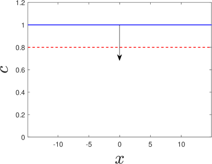
|
\stackinsetl0ptt0pt(b)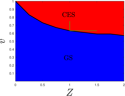
|
\stackinsetl0ptt0pt(c)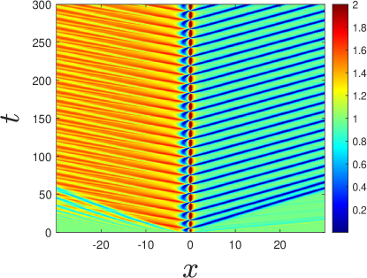
|
\stackinsetl0ptt0pt(d)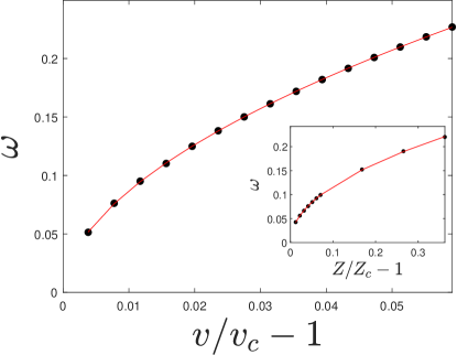
|
This relation is very similar to that between the particle number and phase operators, which we now review following the enlightening discussion of Ref. Mora and Castin (2003). If a phase operator exists, then it satisfies . But
| (135) |
implies that, if is an eigenvalue of , then is also. This violates two fundamental properties of the spectrum of the particle number operator: its positive definiteness and its discreteness. Nevertheless, one can define phase fluctuations in situations involving large particle numbers, where one can neglect the discreteness of the spectrum and states with low occupation number, as in the case of a condensate. In analogy, by identifying energy with particle number and time with phase, one can define time fluctuations for large energies, well above the ground state. Actually, within the formalism, the time operator behaves as a sort of phase operator. This suggests that spontaneous Floquet states should be highly excited states, with a macroscopic energy well above the ground state.
VII Time supersolids: CES state
 |
 |
 |
 |
 |
 |
We now study a specific realization of a spontaneous Floquet state, the so-called CES state de Nova and Sols (2022), which is described by a 1D time-dependent GPG equation (101) of the form:
| (136) |
where the presence of an inhomogeneous external potential explicitly breaks invariance under spatial translations. This guarantees the genuine character of the spontaneous symmetry-breaking of time translation symmetry, avoiding any misidentification of time crystalline behavior as that discussed after Eq. (91). Although the CES state was originally identified from a dynamical phase transition in an analogue gravity context de Nova et al. (2016, 2021), similar scenarios involving soliton emission and periodic self-oscillations are well-known in the literature Hakim (1997); Pavloff (2002); Engels and Atherton (2007); Nguyen et al. (2017); Sels and Demler (2020); Tamura et al. (2023).
In analogy to the case of Sec. IV, the CES state spontaneously breaks and time-translation symmetries. Such a state has been denoted as a time supersolid, combining superfluidity with time crystalline behavior, and has been recently observed in a magnonic BEC Autti et al. (2018). We remark that, while strictly speaking the cnoidal wave is not a supersolid because it is not at equilibrium Martone et al. (2021), time crystals are necessarily out-of-equilibrium states as a consequence of the celebrated no-go theorem Watanabe and Oshikawa (2015).
The CES state satisfies typical time-crystal criteria of robustness, independence from the initial condition, and universality de Nova and Sols (2022). In this work, we focus on a specific realization in which a localized attractive delta barrier is quenched at within a subsonic homogeneous condensate flowing with velocity , described by a GP wavefunction . A schematic depiction of the initial setup is displayed in Fig. 1a. The quench in the external potential induces a deterministic dynamics in the condensate, numerically computed by integrating the time-dependent GP equation (20). The asymptotic behavior of the system is described by a dynamical phase diagram which is a function solely of , Fig. 1b, exhibiting only two possible final states: the nonlinear ground state (GS) Michel and Parentani (2013) or the CES state. Specifically, for initial velocities larger than the critical velocity , or, equivalently, for barrier amplitudes larger than the critical amplitude , the GP condensate wavefunction asymptotically approaches the CES state,
| (137) |
where it oscillates periodically. This periodic behavior is globally displayed both upstream and downstream, as seen in Fig. 1c, and not just in the traveling cnoidal wave downstream (whose time periodicity is rather trivial, as previously argued). We note that the CES state is a macroscopically excited state, as expected from the discussion at the end of Sec. VI.3, since the initial state is shifted an energy with respect to a condensate at rest.
The GS/CES phase diagram is an example of dynamical phase transition Moeckel and Kehrein (2008); Sciolla and Biroli (2010); Lang et al. (2018), where the GS is the symmetry unbroken phase, with continuous time translation symmetry, while the CES state is the time-crystalline phase, with discrete time translation symmetry. The oscillation frequency displays a critical behavior close to the phase boundary, where the critical exponents for (obtained from a fit in Fig. 1d) are both approximately , in agreement with those for a square well de Nova and Sols (2022), potentially suggesting a possible analytical derivation.
 |
 |
We now go beyond mean-field and explicitly compute the dynamics of the quantum fluctuations by using the Truncated Wigner method Sinatra et al. (2002); Carusotto et al. (2008); all technical details behind the numerical simulations and the specific implementation of the Truncated Wigner method can be found in Refs. de Nova et al. (2016); de Nova and Sols (2022, 2023). As initial quantum state, we take the ground state in the comoving frame of the condensate. Regarding the observables of interest, we focus on computing the density-density correlations
| (138) |
with the density fluctuations. In the laboratory, density-density correlations can be measured through in situ imaging after averaging over ensembles of repetitions of the experiment Steinhauer (2016); de Nova et al. (2019); Kolobov et al. (2021).
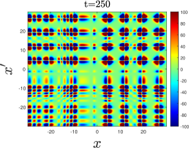
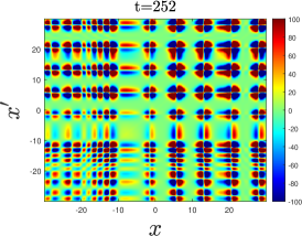
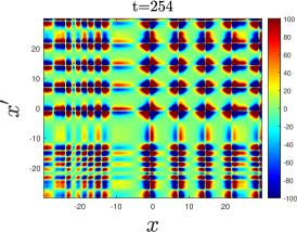
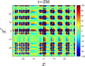
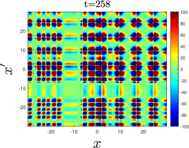
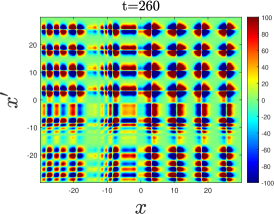
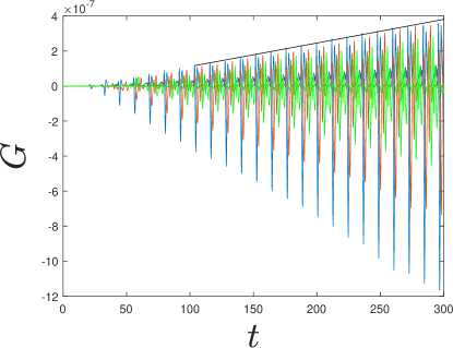
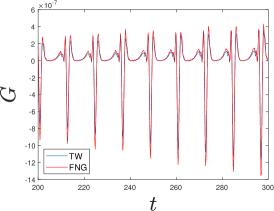
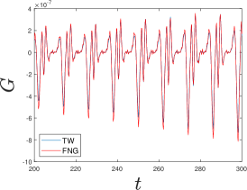
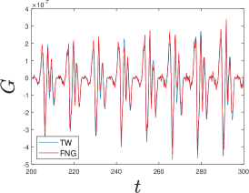
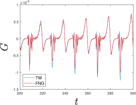
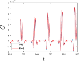
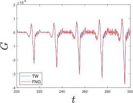
After some transient, and once in the CES state, the correlations exhibit a seemingly periodic behavior, as shown in Fig. 2, where sharp correlation features arise due to the emission of shock waves (solitons) into the upstream (downstream) region. Further insight is obtained in Fig. 3, where we plot the time dependence of the correlations between symmetric upstream and downstream points for different values of , marked as color dots in Fig. 2. We observe that the amplitude of the correlation function is indeed quasi-periodic, with periodic oscillations whose amplitude grows in time.
 |
 |
 |
 |
 |
 |
This behavior can be understood using our spontaneous Floquet theory, developed in Sec. VI. After expanding the field operator around the CES wavefunction as in Eq. (107), we find that the density fluctuations read at linear order in as
| (139) |
Plugging the expansion of Eq. (VI) into this expression yields
with the density amplitude associated to . The FNG mode associated to the phase does not couple to the density, . Thus, only the temporal FNG mode contributes to the correlation function . Moreover, its amplitude grows linearly in time, so it eventually dominates the correlations,
| (141) |
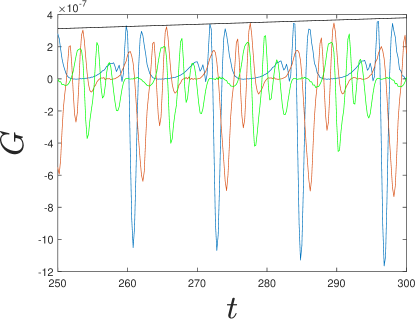
As a result, we expect a quadratic polynomial dependence for , . This fits well the observed growth, black lines in Fig. 3. A more detailed comparison is presented in Fig. 4, where we directly compare the numerical results for from the Truncated Wigner method with the theoretical prediction of Eq. (141), combining the previous fit of with a computation of from the time derivative of the mean-field CES wavefunction itself. A remarkable agreement is observed, confirming the linear growth of the quantum amplitude of the temporal FNG mode as the mechanism responsible for the quasi-periodic correlations.
Based on these results, we propose an experimental scheme to observe the temporal FNG mode using standard techniques in analogue gravity setups Steinhauer (2016); de Nova et al. (2019); Kolobov et al. (2021). We consider an elongated quasi-1D condensate that is essentially homogeneous far from the edges, along which a localized obstacle is swept with velocity . By Galilean invariance, this is equivalent to launching the condensate against the obstacle with the same velocity. For values of above the critical velocity, a CES state will be reached. Another possibility is to confine the condensate in a long ring Eckel et al. (2018) and rotate a localized potential. In both cases, at late times once in the CES regime, when the temporal FNG mode dominates the Bogoliubov dynamics, high-resolution imaging can be then used to measure the time evolution of the density profile and the density-density correlations, from where the FNG mode is extracted as in Fig. 4.
We note that the protocol used here to reach the CES state is fully deterministic at the mean-field level, which fixes the value of the global time origin of the spontaneous Floquet state. Thus, even though there is a temporal FNG mode, technically speaking the symmetry breaking of time translation invariance is not spontaneous. This is because the quenching protocol fixes a origin in the GP equation. However, at late times, due to interactions, the system enters the CES self-oscillating regime where it forgets about the initial condition, exhibiting all the features of a spontaneous Floquet state. We can qualitatively understand this behavior by drawing an analogy with a conventional spatial crystal growing in the -direction on top of a rigid substrate, which fixes a plane that breaks continuous spatial translation symmetry. In the bulk of the grown crystal, the system becomes insensitive to the boundary and recovers the usual properties of a crystalline structure.
Nevertheless, the phase locking of actually helps to measure the FNG mode since, if were spontaneously chosen in each realization of the experiment, then would represent an angular average over , therefore suppressing its time dependence. In that case, one would need to resort to the complete correlation function
| (142) |
which, at the very least, requires the use of non-destructive imaging in order to measure the density at two consecutive times Smits et al. (2018). This distinction is not needed in the usual symmetry breaking, where each realization of the experiment is insensitive to the condensate phase because observables always commute with the total particle number, the generator of global phase transformations.
VIII Discussion and perspectives
We proceed to critically discuss the results of this work and how they inscribe within the literature, exploring in the process futures avenues. We have examined how the general results from Goldstone’s theorem applied to variational descriptions, Sec. II, can be translated to many-body systems when several symmetries are simultaneously broken, focusing on the specific case of a BEC close to zero temperature for illustrative purposes. We have found that the correct description of the problem is provided in terms of the generalized Gibbs ensemble, which treats all broken symmetries on equal grounds. The Lagrange multipliers associated to each conserved charge behave as generalized velocities along the orbits of the symmetry transformations, extending the well-known result that the chemical potential is the velocity of the phase. We also prove fundamental results in Thermodynamics for the symmetry-broken state, such as the first principle and the Gibbs-Duhem relation.
The Nambu-Goldstone modes associated to each spontaneous symmetry-breaking emerge as zero-energy modes of the Bogoliubov spectrum. Each Nambu-Goldstone mode is paired with a Gibbs mode, arising from fluctuations of the condensate wavefunction with respect to the corresponding conserved charge. Interestingly, the orthogonalization of the Goldstone-Gibbs sector involves the Berry-Gibbs connection, which is the usual Berry connection when applied to the macroscopic condensate wavefunction, here depending on the conserved charges, which are not intrinsic parameters of the Hamiltonian. This geometrical interpretation is extended to describe the quantization of the amplitudes of the Nambu-Goldstone/Gibbs modes using a symplectic structure, finding that they behave as coordinate/momentum operators. This relation is also observed in the dynamics, where the momenta are conserved due to the symmetries of the Hamiltonian, while the coordinates grow linearly in time with velocities proportional to the momenta. Finally, we show that the Goldstone-Gibbs sector can be diagonalized, leading to a new set of independent Nambu-Goldstone modes. Remarkably, this diagonalization only involves thermodynamic considerations, and describes how the original Nambu-Goldstone modes mix within the different Bogoliubov branches in the low-frequency limit.
The coordinate-momentum analogy between the NG and the Gibbs amplitude was originally established in Ref. Lewenstein and You (1996) in the context of the -symmetry breaking and the phase diffusion of a condensate. This approach was extended in Ref. Dziarmaga (2004) to also quantize the position of a soliton and study its quantum diffusion. The present work generalizes those approaches to an arbitrary number of spontaneously broken symmetries, providing a general and systematic framework with the help of the generalized Gibbs ensemble and the Berry-Gibbs connection, which in addition allows to understand the role of the Nambu-Goldstone and Gibbs modes at a more fundamental level. To the best of our knowledge, the framework developed in Sec. III is original from this work and not present in the literature.
As a particular application of the developed formalism, we have studied in Sec. IV the case of a cnoidal wave in a superfluid, which spontaneously breaks and spatial translation symmetry, extending the work of Refs. Dziarmaga (2004); Martone et al. (2021) into the generalized Gibbs ensemble. We have explicitly checked the validity of the predictions of Sec. III.
The results of Secs. III, IV can then be of interest for the study of systems which spontaneously break several symmetries, such as supersolids Léonard et al. (2017); Li et al. (2017) or quantum droplets Chomaz et al. (2016); Cabrera et al. (2018); Zin et al. (2021). However, the generality of the formalism allows for a straightforward adaptation to other systems. For instance, within the quantum Hall phase diagram in graphene, states with two spontaneously broken symmetries were predicted within a HF description de Nova and Zapata (2017), of which some experimental evidence was recently reported Coissard et al. (2022). Indeed, Ref. de Nova and Zapata (2017) established the correspondence between the BdG and TDHFA equations, and translated Goldstone theorem to the specific context of the HF equations using similar techniques to those of this work.
The formalism developed for stationary states in Secs. II-III is adapted to spontaneous Floquet states in Secs. V, VI. Specifically, from the general results of Sec. II, we prove that the usual Nambu-Goldstone modes with zero energy are now translated into Floquet-Nambu-Goldstone modes with zero quasi-energy. Moreover, since spontaneous Floquet states break time-translational symmetry, a genuine temporal Floquet-Nambu-Goldstone mode emerges. This is a distinctive signature of a spontaneous Floquet state, completely absent in conventional Floquet systems.
In order to correctly describe the dynamics of spontaneous Floquet states, we develop what we denote as the formalism, which extends the usual formalism. In combination with the generalized Gibbs ensemble, we provide a thermodynamical description of spontaneous Floquet states analogous to that of stationary states, which we denote as Floquet thermodynamics. This is possible because spontaneous Floquet states also have a well-defined energy, which enables the existence of the Floquet charge. The Floquet thermodynamics is another hallmark of spontaneous Floquet states, in addition to the presence of a temporal Floquet-Nambu-Goldstone mode. In fact, both features are the sides of the same coin, since they arise, via Goldstone and Noether theorems, from the continuous time-translation symmetry of the underlying time-independent Hamiltonian.
The quantization procedure of the FNG modes goes along the same lines as in the stationary case, involving a Berry-Gibbs connection and a symplectic form. Nevertheless, we now have a novel temporal FNG mode, whose amplitude can be regarded as an effective time coordinate, with a conjugate momentum given by the energy fluctuations. Therefore, we can identify the quantum amplitude of the temporal FNG mode as a rare realization of a time operator in Quantum Mechanics.
We stress that the use of the generalized Gibbs ensemble in combination with the formalism is essential for a correct description of the problem. Interestingly, within this framework, a remarkable correspondence between stationary states and spontaneous Floquet states can be established, consisting of replacing stationary states by periodic states, frequencies by quasi-frequencies, and conserved charges by their angular average.
Finally, we apply our formalism to a specific realization of spontaneous Floquet state, the CES state, which spontaneously breaks and continuous time-translation symmetry, behaving as a time supersolid. We propose an experimental scheme, based on standard analogue gravity techniques Steinhauer (2016); de Nova et al. (2019); Kolobov et al. (2021), to observe the temporal FNG mode, which does couple to the density in contrast to the usual FNG mode associated to the phase. In particular, we predict that the density-density correlations are dominated at late times by the growth of the FNG mode, from where it can be extracted. Numerical results from a Truncated Wigner simulation show a remarkable agreement with the theory.
The results of Secs. V-VII can be used to describe simultaneous symmetry breaking in conventional Floquet systems. They also find a major application in the field of time crystals, since a spontaneous Floquet state represents a particular realization of a continuous time crystal Wilczek (2012); Autti et al. (2018); Kongkhambut et al. (2022); Greilich et al. (2024). Indeed, an important point of the analysis presented in Sec. IV is that it suggests that certain periodic systems identified as time crystals may not genuinely break continuous time translation symmetry, such as constant motion along a ring. Thus, the observation of a genuine temporal FNG mode, arising from a spontaneous breaking of continuous time-translation symmetry, should be regarded as a characteristic signature of any bona fide time crystal.
Some other results of our work are connected with the time crystal literature. For instance, the role of the generalized Gibbs ensemble in dissipative time crystals was thoroughly discussed in Ref. Booker et al. (2020). The emergence of continuous time crystals from excited eigenstates, in the same fashion as spontaneous Floquet states, was already predicted in Ref. Syrwid et al. (2017). Time supersolids, like the CES state, were originally observed in Ref. Autti et al. (2018).
Although we have focused on atomic condensates, our Floquet formalism can be also extrapolated to magnonic condensates Mäkinen et al. (2023). In general, spontaneous Floquet states extend the field of nonlinear Floquet waves Kreil et al. (2019); Träger et al. (2021) to scenarios without external driving. Nonlinear optical fibers Drummond and Hillery (2014) and quantum fluids of light Carusotto and Ciuti (2013) are also natural candidates to exhibit spontaneous Floquet states, since they obey equations of motion similar to the GP equation. Spontaneous Floquet states in fermionic systems described by HF approaches, such as quantum Hall states, are also plausible. There, our formalism can be straightforwardly adapted due to the BdG/TDHFA correspondence de Nova and Zapata (2017). In addition, self-consistent BCS-type theories are known to display periodic oscillations in momentum space Barankov et al. (2004); Foster et al. (2014); Perfetto and Stefanucci (2020).
Future extensions of the present work should include finite temperature effects and quantum corrections beyond linearity, both for stationary and spontaneous Floquet states exhibiting simultaneous symmetry breaking. Of particular interest is the general study of the quantum diffusion of the spontaneously broken symmetries, generalizing the works of Refs. Lewenstein and You (1996); Dziarmaga (2004). In the case of the temporal Floquet-Nambu-Goldstone mode, this could lead to suggestive concepts such as time diffusion or time eigenstates, in analogy with the phase of a condensate Leggett and Sols (1991); Sols (1994). A subject of ongoing research de Nova et al. is the achievement of a fully quantum time crystal from the CES state that spontaneously breaks time-translation symmetry, without phase locking its time origin as in the present work. This can be done by either approaching the GS-CES phase transition, where quantum fluctuations become critical, or by starting from a quantum black-hole laser de Nova and Sols (2023).
Acknowledgements.
We thank C. Cabrera and M. A. García-March for useful discussions. This project has received funding from European Union’s Horizon 2020 research and innovation programme under the Marie Skłodowska-Curie Grant Agreement No. 847635, from Spain’s Agencia Estatal de Investigación through Grant No. PID2022-139288NB-I00, and from Universidad Complutense de Madrid through Grant No. FEI-EU-19-12.Appendix A Cnoidal waves in the GPG equation
A.1 Elliptic functions
We briefly review here some basic notions of elliptic functions. We begin by defining the Jacobi elliptic functions
| (143) |
where is the inverse function of the incomplete elliptic integral of the first kind for fixed ,
| (144) |
In turn, the incomplete and complete elliptic integrals of the first kind are
| (145) |
As a consequence of these relations, , and thus are periodic functions with period . The complete and incomplete elliptic integrals of the second kind are
| (146) |
Finally, the incomplete and complete elliptic integrals of the third kind are
| (147) |
Of interest are also the integrals
| (148) | |||||
which appear when evaluating the particle number or the energy of a cnoidal wave. They can be shown to obey the inter-recursive relations:
| (149) | |||||
which yield
| (150) |
with .
A.2 GPG solutions in a ring
Since the GPG equation can be rewritten as Eq. (78), we first study in detail the solutions to the stationary GP equation
| (151) |
This equation is solved by decomposing the wavefunction in amplitude and phase as , finding
| (152) | |||||
The second equation simply yields the conservation of the current, , with the 1D density and the flow velocity. When plugged into the first equation, we obtain something of the form , which can be thought as the equation of motion of a fictitious particle in a potential , where plays here the role of time. Energy conservation then implies:
| (153) | |||||
Using instead the density , we find that the wavefunction is determined by the set of differential equations
| (154) |
where the three densities , , are the roots of the polynomial
| (155) |
These densities are related to the more physical chemical potential , the particle current , and the amplitude energy as
| (156) | |||||
Finally, one integrates first the equation for in Eq. (154) and then that of the phase, obtaining the cnoidal wave (79). From its expression, we can compute the pure cnoidal contribution to the momentum
| (157) |
Since , it is immediately found that the total momentum is simply
| (158) |
Moreover, , and thus the total particle number is directly obtained from the integral of the cnoidal density. With the help of these results, one arrives at Eq. (87). The trick to solve that equation is to express all roots in terms of , , achieving thus a equation for a single real parameter . For that purpose, one combines the first two lines of Eq. (87) to express in terms of , and invokes the definition of itself, Eq. (80), to obtain . Inserting these results into the third line of Eq. (87) yields a single equation for , which can be easily numerically solved as . Once is obtained, the densities are computed, and the complete GPG wavefunction and the total energy are determined.
Finally, we show that the Berry-Gibbs connection (52) automatically vanishes in our gauge choice. By decomposing the GPG wavefunction in phase and amplitude, , it is easily seen that in general
| (159) |
In the specific case of the 1D GPG cnoidal wave, Eq. (85), . Moreover, the second line of Eq. (86),
| (160) |
imposes that the crystal momentum is fixed by the winding number and does not depend on the charges, so . As in our particular gauge is an even periodic function, then is an odd periodic function, and thus identically vanishes by parity symmetry.
References
- Callen (1985) H. B. Callen, Thermodynamics and an Introduction to Thermostatistics (Wiley, New York, 1985).
- Léonard et al. (2017) J. Léonard, A. Morales, P. Zupancic, T. Esslinger, and T. Donner, Nature 543, 87 (2017).
- Li et al. (2017) J.-R. Li, J. Lee, W. Huang, S. Burchesky, B. Shteynas, F. Ç. Top, A. O. Jamison, and W. Ketterle, Nature 543, 91 (2017).
- Chomaz et al. (2016) L. Chomaz, S. Baier, D. Petter, M. J. Mark, F. Wächtler, L. Santos, and F. Ferlaino, Phys. Rev. X 6, 041039 (2016).
- Cabrera et al. (2018) C. R. Cabrera, L. Tanzi, J. Sanz, B. Naylor, P. Thomas, P. Cheiney, and L. Tarruell, Science 359, 301 (2018).
- Zin et al. (2021) P. Zin, M. Pylak, and M. Gajda, New Journal of Physics 23, 033022 (2021).
- Wilczek (2012) F. Wilczek, Phys. Rev. Lett. 109, 160401 (2012).
- Watanabe and Oshikawa (2015) H. Watanabe and M. Oshikawa, Phys. Rev. Lett. 114, 251603 (2015).
- Choi et al. (2017) S. Choi, J. Choi, R. Landig, G. Kucsko, H. Zhou, J. Isoya, F. Jelezko, S. Onoda, H. Sumiya, V. Khemani, et al., Nature 543, 221 (2017).
- Zhang et al. (2017) J. Zhang, P. Hess, A. Kyprianidis, P. Becker, A. Lee, J. Smith, G. Pagano, I.-D. Potirniche, A. C. Potter, A. Vishwanath, et al., Nature 543, 217 (2017).
- Smits et al. (2018) J. Smits, L. Liao, H. T. C. Stoof, and P. van der Straten, Phys. Rev. Lett. 121, 185301 (2018).
- Rovny et al. (2018) J. Rovny, R. L. Blum, and S. E. Barrett, Phys. Rev. Lett. 120, 180603 (2018).
- Kyprianidis et al. (2021) A. Kyprianidis, F. Machado, W. Morong, P. Becker, K. S. Collins, D. V. Else, L. Feng, P. W. Hess, C. Nayak, G. Pagano, N. Y. Yao, and C. Monroe, Science 372, 1192 (2021).
- Randall et al. (2021) J. Randall, C. E. Bradley, F. V. van der Gronden, A. Galicia, M. H. Abobeih, M. Markham, D. J. Twitchen, F. Machado, N. Y. Yao, and T. H. Taminiau, Science 374, 1474 (2021).
- Mi et al. (2022) X. Mi, M. Ippoliti, C. Quintana, A. Greene, Z. Chen, J. Gross, F. Arute, K. Arya, J. Atalaya, R. Babbush, et al., Nature 601, 531 (2022).
- Frey and Rachel (2022) P. Frey and S. Rachel, Science Advances 8, eabm7652 (2022).
- Autti et al. (2018) S. Autti, V. B. Eltsov, and G. E. Volovik, Phys. Rev. Lett. 120, 215301 (2018).
- Kongkhambut et al. (2022) P. Kongkhambut, J. Skulte, L. Mathey, J. G. Cosme, A. Hemmerich, and H. Keßler, Science 377, 670 (2022).
- Liu et al. (2023) T. Liu, J.-Y. Ou, K. F. MacDonald, and N. I. Zheludev, Nature Physics , 1 (2023).
- Greilich et al. (2024) A. Greilich, N. Kopteva, A. Kamenskii, P. Sokolov, V. Korenev, and M. Bayer, Nature Physics , 1 (2024).
- Sacha (2015) K. Sacha, Phys. Rev. A 91, 033617 (2015).
- Else et al. (2016) D. V. Else, B. Bauer, and C. Nayak, Phys. Rev. Lett. 117, 090402 (2016).
- Shirley (1965) J. H. Shirley, Phys. Rev. 138, B979 (1965).
- Sambe (1973) H. Sambe, Phys. Rev. A 7, 2203 (1973).
- Grifoni and Hänggi (1998) M. Grifoni and P. Hänggi, Physics Reports 304, 229 (1998).
- Peng et al. (2021) P. Peng, C. Yin, X. Huang, C. Ramanathan, and P. Cappellaro, Nature Physics 17, 444 (2021).
- Lindner et al. (2011) N. H. Lindner, G. Refael, and V. Galitski, Nature Physics 7, 490 (2011).
- Prosen and Ilievski (2011) T. c. v. Prosen and E. Ilievski, Phys. Rev. Lett. 107, 060403 (2011).
- Murakami et al. (2018) Y. Murakami, M. Eckstein, and P. Werner, Phys. Rev. Lett. 121, 057405 (2018).
- Pieplow et al. (2019) G. Pieplow, C. E. Creffield, and F. Sols, Phys. Rev. Res. 1, 033013 (2019).
- Mateos et al. (2023) J. Mateos, C. E. Creffield, and F. Sols, New Journal of Physics 25, 063006 (2023).
- de Nova and Sols (2022) J. R. M. de Nova and F. Sols, Phys. Rev. A 105, 043302 (2022).
- de Nova et al. (2016) J. R. M. de Nova, S. Finazzi, and I. Carusotto, Phys. Rev. A 94, 043616 (2016).
- de Nova et al. (2021) J. R. M. de Nova, P. F. Palacios, I. Carusotto, and F. Sols, New Journal of Physics 23, 023040 (2021).
- Cazalilla (2006) M. A. Cazalilla, Phys. Rev. Lett. 97, 156403 (2006).
- Rigol et al. (2007) M. Rigol, V. Dunjko, V. Yurovsky, and M. Olshanii, Phys. Rev. Lett. 98, 050405 (2007).
- Langen et al. (2015) T. Langen, S. Erne, R. Geiger, B. Rauer, T. Schweigler, M. Kuhnert, W. Rohringer, I. E. Mazets, T. Gasenzer, and J. Schmiedmayer, Science 348, 207 (2015).
- Lewenstein and You (1996) M. Lewenstein and L. You, Phys. Rev. Lett. 77, 3489 (1996).
- Dziarmaga (2004) J. Dziarmaga, Phys. Rev. A 70, 063616 (2004).
- Peskin and Moiseyev (1993) U. Peskin and N. Moiseyev, The Journal of Chemical Physics 99, 4590 (1993).
- Heimsoth et al. (2012) M. Heimsoth, C. Creffield, L. Carr, and F. Sols, New Journal of Physics 14, 075023 (2012).
- Sinatra et al. (2002) A. Sinatra, C. Lobo, and Y. Castin, J. Phys. B: At. Mol. Opt. Phys 35, 3599 (2002).
- Carusotto et al. (2008) I. Carusotto, S. Fagnocchi, A. Recati, R. Balbinot, and A. Fabbri, New J. Phys. 10, 103001 (2008).
- Steinhauer (2016) J. Steinhauer, Nature Physics 12, 959 (2016).
- de Nova et al. (2019) J. R. M. de Nova, K. Golubkov, V. I. Kolobov, and J. Steinhauer, Nature 569, 688 (2019).
- Kolobov et al. (2021) V. I. Kolobov, K. Golubkov, J. R. M. de Nova, and J. Steinhauer, Nature Physics 17, 362 (2021).
- Goldstone et al. (1962) J. Goldstone, A. Salam, and S. Weinberg, Phys. Rev. 127, 965 (1962).
- DeAngelis and Gatoff (1991) A. R. DeAngelis and G. Gatoff, Phys. Rev. C 43, 2747 (1991).
- Pitaevskii and Stringari (2016) L. Pitaevskii and S. Stringari, Bose-Einstein Condensation and superfluidity (Clarendon Press, Oxford, 2016).
- Giuliani and Vignale (2005) G. Giuliani and G. Vignale, Quantum Theory of the Electron Liquid, Masters Series in Physics and Astronomy (Cambridge University Press, 2005).
- Jaksch et al. (1998) D. Jaksch, C. Bruder, J. I. Cirac, C. W. Gardiner, and P. Zoller, Phys. Rev. Lett. 81, 3108 (1998).
- Caillat et al. (2005) J. Caillat, J. Zanghellini, M. Kitzler, O. Koch, W. Kreuzer, and A. Scrinzi, Phys. Rev. A 71, 012712 (2005).
- Alon et al. (2008) O. E. Alon, A. I. Streltsov, and L. S. Cederbaum, Phys. Rev. A 77, 033613 (2008).
- Caleffi et al. (2020) F. Caleffi, M. Capone, C. Menotti, I. Carusotto, and A. Recati, Phys. Rev. Research 2, 033276 (2020).
- Thouless (2014) D. J. Thouless, The quantum mechanics of many-body systems (Courier Corporation, 2014).
- Fetter and Walecka (2003) A. Fetter and J. Walecka, Quantum Theory of Many-particle Systems, Dover Books on Physics (Dover Publications, 2003).
- Menotti and Stringari (2002) C. Menotti and S. Stringari, Phys. Rev. A 66, 043610 (2002).
- Martone et al. (2021) G. I. Martone, A. Recati, and N. Pavloff, Phys. Rev. Res. 3, 013143 (2021).
- Lignier et al. (2007) H. Lignier, C. Sias, D. Ciampini, Y. Singh, A. Zenesini, O. Morsch, and E. Arimondo, Phys. Rev. Lett. 99, 220403 (2007).
- Kierig et al. (2008) E. Kierig, U. Schnorrberger, A. Schietinger, J. Tomkovic, and M. K. Oberthaler, Phys. Rev. Lett. 100, 190405 (2008).
- Gaul et al. (2011) C. Gaul, E. Díaz, R. P. A. Lima, F. Domínguez-Adame, and C. A. Müller, Phys. Rev. A 84, 053627 (2011).
- Rapp et al. (2012) A. Rapp, X. Deng, and L. Santos, Phys. Rev. Lett. 109, 203005 (2012).
- Stöferle et al. (2004) T. Stöferle, H. Moritz, C. Schori, M. Köhl, and T. Esslinger, Phys. Rev. Lett. 92, 130403 (2004).
- Mora and Castin (2003) C. Mora and Y. Castin, Phys. Rev. A 67, 053615 (2003).
- Hakim (1997) V. Hakim, Phys. Rev. E 55, 2835 (1997).
- Pavloff (2002) N. Pavloff, Phys. Rev. A 66, 013610 (2002).
- Engels and Atherton (2007) P. Engels and C. Atherton, Phys. Rev. Lett. 99, 160405 (2007).
- Nguyen et al. (2017) J. H. V. Nguyen, D. Luo, and R. G. Hulet, Science 356, 422 (2017).
- Sels and Demler (2020) D. Sels and E. Demler, Annals of Physics 412, 168021 (2020).
- Tamura et al. (2023) H. Tamura, S. Khlebnikov, C.-A. Chen, and C.-L. Hung, arXiv preprint arXiv:2304.10667 (2023).
- Michel and Parentani (2013) F. Michel and R. Parentani, Phys. Rev. D 88, 125012 (2013).
- Moeckel and Kehrein (2008) M. Moeckel and S. Kehrein, Phys. Rev. Lett. 100, 175702 (2008).
- Sciolla and Biroli (2010) B. Sciolla and G. Biroli, Phys. Rev. Lett. 105, 220401 (2010).
- Lang et al. (2018) J. Lang, B. Frank, and J. C. Halimeh, Phys. Rev. Lett. 121, 130603 (2018).
- de Nova and Sols (2023) J. R. M. de Nova and F. Sols, Phys. Rev. Res. 5, 043282 (2023).
- Eckel et al. (2018) S. Eckel, A. Kumar, T. Jacobson, I. B. Spielman, and G. K. Campbell, Phys. Rev. X 8, 021021 (2018).
- de Nova and Zapata (2017) J. R. M. de Nova and I. Zapata, Phys. Rev. B 95, 165427 (2017).
- Coissard et al. (2022) A. Coissard, D. Wander, H. Vignaud, A. G. Grushin, C. Repellin, K. Watanabe, T. Taniguchi, F. Gay, C. B. Winkelmann, H. Courtois, et al., Nature 605, 51 (2022).
- Booker et al. (2020) C. Booker, B. Buča, and D. Jaksch, New Journal of Physics 22, 085007 (2020).
- Syrwid et al. (2017) A. Syrwid, J. Zakrzewski, and K. Sacha, Phys. Rev. Lett. 119, 250602 (2017).
- Mäkinen et al. (2023) J. T. Mäkinen, S. Autti, and V. B. Eltsov, arXiv preprint arXiv:2312.10119 (2023).
- Kreil et al. (2019) A. J. E. Kreil, H. Y. Musiienko-Shmarova, S. Eggert, A. A. Serga, B. Hillebrands, D. A. Bozhko, A. Pomyalov, and V. S. L’vov, Phys. Rev. B 100, 020406 (2019).
- Träger et al. (2021) N. Träger, P. Gruszecki, F. Lisiecki, F. Groß, J. Förster, M. Weigand, H. Głowiński, P. Kuświk, J. Dubowik, G. Schütz, M. Krawczyk, and J. Gräfe, Phys. Rev. Lett. 126, 057201 (2021).
- Drummond and Hillery (2014) P. D. Drummond and M. Hillery, The quantum theory of nonlinear optics (Cambridge University Press, 2014).
- Carusotto and Ciuti (2013) I. Carusotto and C. Ciuti, Rev. Mod. Phys. 85, 299 (2013).
- Barankov et al. (2004) R. A. Barankov, L. S. Levitov, and B. Z. Spivak, Phys. Rev. Lett. 93, 160401 (2004).
- Foster et al. (2014) M. S. Foster, V. Gurarie, M. Dzero, and E. A. Yuzbashyan, Phys. Rev. Lett. 113, 076403 (2014).
- Perfetto and Stefanucci (2020) E. Perfetto and G. Stefanucci, Phys. Rev. Lett. 125, 106401 (2020).
- Leggett and Sols (1991) A. J. Leggett and F. Sols, Foundations of physics 21, 353 (1991).
- Sols (1994) F. Sols, Physica B: Condensed Matter 194, 1389 (1994).
- (91) J. R. M. de Nova et al., to be published .
