Autonomous Emergency Braking With Driver-In-The-Loop: Torque Vectoring for Active Learning

Abstract

Autonomous Emergency Braking (AEB) potentially brings significant improvements in automotive safety due to its ability to autonomously prevent collisions in situations where the driver may not be able to do so. Driven by the poor performance of the state of the art in recent testing, this work provides an online solution to identify critical parameters such as the current and maximum friction coefficients. The method introduced here, namely Torque Vectoring for Active Learning (TVAL), can perform state and parameter estimation whilst following the driver’s input. Importantly with less power requirements than normal driving. Our method is designed with a crucial focus on ensuring minimal disruption to the driver, allowing them to maintain full control of the vehicle. Additionally, we exploit a rain/light sensor to drive the observer resampling to maintain estimation certainty across prolonged operation. Then a scheme to modulate TVAL is introduced that considers powertrain efficiency, safety, and availability in an online fashion. Using a high-fidelity vehicle model and drive cycle we demonstrate the functionality of TVAL controller across changing road surfaces where we successfully identify the road surface whenever possible.

I Introduction

Autonomous Emergency Braking (AEB) systems are gradually penetrating into main stream, mass production vehicles. However literature is limited with significant problems reported in testing of commercial systems. Recent (2022) testing conducted by the American Automobile Association (AAA) and National Highway Traffic Safety Administration (NHTSA) found that, at an approach speed of $40mph$, AEB systems only prevented $30\%$ of collisions and in some common scenarios, preventing collisions was not achieved at all [1]. To achieve safe control of a vehicle, the tyre-road surface interaction is critical to understand in real time. Advanced Driver Assistance features, such as the Anti-Lock Brake system (ABS) [2] or Electronic Stability Control (ESC) are required to control the vehicle at the limits of adhesion which can rely on accurate identification of the vehicle states and tyre model when maximizing the tyre friction. In the case of more automated or autonomous features, such as AEB, this information must be known prior to the emergency braking and with a high degree of confidence to avoid collision. Overestimation of the current and maximum achievable friction leads to collision since the controller believes that greater deceleration is possible. Under-estimation results in poor confidence and creates a lack of trust from the driver in the vehicles active safety features, potentially leading to misuse or deactivation. The optimal identification of the tyre model and road surface is challenged by the wide range of operating conditions a typical vehicle may experience. These include changing road surfaces e.g. from dry to wet to ice, then the tyre itself may behave differently due to tread wear, temperature or inflation variations and the vehicle may operate at across a wide range of states such as high or low velocities. Our method, namely Torque Vectoring for Active Learning (TVAL) addresses these obstacles and identifies both the current and maximum friction coefficient whilst reducing the uncertainty. Since there is emphasis on having a high degree of confidence required to take control of the vehicle during an emergency. Critically, our method performs identification before an emergency situation and can be used to accurately identify the optimal stopping distance while minimizing any perturbations on the driver.

While direct observation of the friction coefficient through tire force sensors, as demonstrated in [3], is possible, it proves prohibitively expensive and impractical for mass production vehicles. Our work establishes that such an approach is unnecessary, since we achieve comparable results with low-cost, readily available sensors. Friction estimation is primarily considered by existing research using passive means, that is, using the input from the driver to learn the friction state. These use either local (effect) methods to estimate the current friction at the tyre contact patch, or predictive (causal) methods to find the future maximum friction coefficient. Predictive methods overwhelmingly utilize cameras e.g. [4], to identify and segment the road surface according to its friction properties. It has been acknowledged that optical based methods alone are unable to determine the friction coefficient with sufficient accuracy [5]. These methods largely rely on classifying road conditions into a limited set of categories with attributed friction properties. In practice, this approach can lead to substantial estimation errors. For example, a wet road may have a maximum friction coefficient between $0.3-0.9$ [6]. In [7] the road type classification using 5 categories of road surface is demonstrated to have an accuracy of 95%. [8] developed an AEB estimation method to jointly estimate the road grade and road type using dry, wet or snow classifiers with between $75\%-85\%$ identification success.

Early methods for local friction estimation initially focused on whole vehicle friction estimation, providing an average estimate for the whole vehicle, as seen in works such as [9] [10]. This approach later evolved into methods that target individual wheel estimation e.g. [11]. In [12], a Kalman Filter was used to directly identify the current tyre friction coefficient but without identifying a tyre model. A novel tyre model was developed in [13] and was successfully identified using a Square Root Cubature Kalman Filter but requires manufacturers to parameterize their tyres according to the new model. Similarly [14] presents an offline method using 3 minutes of drifting making it unsuitable for normal driving. Others identified the Brush tyre model which requires fewer parameters but comes at the expense of accuracy [15]. In comparison, our work identifies the widely accepted Magic Formula tyre model which can model a large range of tyres.

Although there has been significant interest in passive identification methods that use normal driver inputs to identify the friction coefficients, active methods, where additional vehicle inputs such as braking or driving torque are necessary for identification at large slip angles. This is particularly necessary where the relationship becomes nonlinear (where peak friction occurs). Active learning through tyre force excitation is known to improve the estimation quality [16]. However very few researchers acknowledge this by designing active learning friction identification methods. The aim of these methods is to perturb the behavior of the wheel above what the driver provides as inputs to the vehicle but without disturbing the driver. The authors of [17] acknowledge this and investigate how different excitation strategies influence the identification accuracy for longitudinal only vehicular motion. Although yielding useful insights, such as the choice of tyre model required different levels of excitation to achieve suitable accuracy, with the Magic formula requiring the lowest level of excitation, this optimization approach is not suitable for real-time control as it is limited by its batch approach. This work does not consider when tyre force excitation should commence and provides a barrier for physical implementation since it may not be safe to always be actively exciting the vehicle, although is addressed in our work. An approach using PID control is shown in [18], but it only tracks a step torque input which is supplied to each wheel (with opposite signs) and achieves an acceleration error of $0.7m/s^{2}$. Since opposite torques are used, tyre forces become unbalanced at high values of slip and asymmetric vehicle loading. An offline nonlinear least squares method was used to fit the measurements to a brush tyre model. Among the literature surveyed, none of the methods accomplishes this identification whilst considering a non-zero acceleration input from the driver; however, our method successfully achieves this capability.

In this regard, our method is well equipped to work with similar vehicle control systems that utilize torque vectoring, namely those used for stability control, which has increased growth in the last 5 years due to the adaptation of electrified vehicles [19]. These methods encounter challenges as they necessitate highly accurate prior tire and vehicle information for effective operation.

The contributions of this work are as follows. We present a novel TVAL control scheme (see Fig. 1) that identifies the current and maximum road surface friction coefficients while following the driver’s input. This is done by identifying the parameters of the Magic formula in a gain free manner. Unique to this work, rain/light sensor (used for windscreen wipers) is used as part of a resampling scheme to drive the on-line estimator. Then, we introduce a new method for regulating active learning by incorporating considerations of tyre force availability, energy efficiency and safety. This enhancement significantly augments the applicability of the scheme for real world deployment. Notably, a hysteresis switch-based strategy for intelligently distinguishing when TVAL can improve the system belief of the peak friction coefficient is presented. An approach for predicting the understeer gradient of a vehicle during TVAL is also utilised, effectively mitigating instability caused by unexpected lateral disturbances. A smooth transition between active learning and purely driver inputs is also introduced. Finally, the complete control scheme is demonstrated in simulation using a 7DOF vehicle dynamics model of a Jaguar XE and a driver model. Here a mixture of road surfaces, including dry, wet, and snowy road surfaces, is investigated in simulation.

The rest of the paper is organized as follows. In Section II the vehicles dynamic and tyre model are presented. Then in Section III a motivation for active learning is shown with TVAL being introduced in Section IV. Section V presents the TVAL modulation approach with the full TVAL scheme demonstrated in simulation in Section VI and conclusions in Section VII.

Figure 1: TVAL system architecture for AEB with the novel contribution shown in red. A Global Navigation Satellite System (GNSS) e.g. GPS gives vehicle speed measurements and Dual Control for Exploration-Exploitation (DCEE) is used as part of our control strategy.

II Vehicle Dynamics

This work focuses on the braking only behaviour of the vehicle, hence an 7 DOF model (see Fig. 2) is presented including the suspension dynamics with bounce and pitching moments. The model presented here follows the SAE (Society of Automotive Engineers) frame of reference [20] and validated against a real vehicle [21] using parameters in [2].

Figure 2: 7 DOF vehicle dynamics model.

II-A Vehicle body

The contribution of all longitudinal ($x$ direction) and vertical ($z$ direction) tyre forces $F_{x,j}$ is found using the vehicle mass $m$ while considering the movement of the centre of gravity (COG), denoted as $\left[x_{G},y_{G},z_{G}\right]$, indicating

$$\sum^{4}_{j=1}F_{x,j}=m\left(\frac{dU}{dt}+Wq\right)-m\left(x_{G}q^{2}-z_{G}\frac{dq}{dt}\right)$$ (1)

$$\sum^{4}_{j=1}F_{z,j}=m\left(\frac{dW}{dt}-Uq\right)-m\left(z_{G}q^{2}+x_{G}\frac{dq}{dt}\right)$$ (2)

where $U$ and $W$ are the velocities of the vehicle body (at the COG) in the longitudinal and vertical directions, $q$ is the rate of change in pitch of the vehicle body and $j$ denotes the location of the wheel, i.e, $j\in\left[1,2,3,4\right]$. Furthermore, the rotation about the y-axis can be calculated by (3) using the moment of inertia about the $yy$ axis, $I_{yy}$. The moments produced by the forces at each wheel, $M_{y,j}$ are found as:

$$\sum^{4}_{j=1}M_{y,j}=I_{yy}\frac{dq}{dt}+mz_{G}\left(\frac{dU}{dt}+Wq\right)-mx_{G}\left(\frac{dW}{dt}-Uq\right)$$ (3)

Next we introduce the suspension model as a mass-spring damper using spring stiffnesses for the front and rear $k_{f,r}$ and damping coefficient $c_{f,r}$:

$$F_{z,f}=k_{\mathrm{f}}\left(z_{G}-|a|\phi\right)+c_{\mathrm{f}}\left(W-|a|q\right)$$ (4)

$$F_{z,r}=k_{\mathrm{r}}\left(z_{G}+|b|\phi\right)+c_{\mathrm{r}}\left(W+|b|q\right)$$ (5)

where $a$ and $b$ are the distances between the front and rear axles to the COG such that the sum is equal to the wheelbase $l$. Additionally the pitch angle is denoted as $\phi$.

II-B Wheels and Tyre Model

The wheel dynamics are found using the wheel rotational acceleration, $\dot{\omega}_{j}$ and the contribution from braking or accelerating the vehicle, applied as torque $T_{j}$. Hence,

$$I_{w}\dot{\omega}_{j}=T_{j}-RF_{x,j},$$ (6)

where $I_{w,j}$ is the wheel inertia and $R$ is the radius of the wheel. The tyre force is simply the product of the wheel vertical load and the friction coefficient between the tyre and road surface:

$$F_{x,j}=\mu(\kappa_{j})F_{z,j}.$$ (7)

In this work the Magic formula tyre model is used with parameters $B,C,D$ and $E$ that are the stiffness, shape, peak and curvature factors respectively, as

$$\mu_{j}=D\sin[C\arctan({B\kappa_{j}-E(B\kappa_{j}-\arctan B\kappa_{j})})]$$ (8)

Note that we consider a single tyre model for all four tyres, but each wheel slip is independent from one another. Using this tyre model allows for the encompassment of many different tyres on different road surfaces including dry, wet and snow. Then the longitudinal slip ratio, $\kappa_{j}$, is generated as the tyre carcass begins to deform because of the difference in linear speed of rolling and body velocity:

$$\kappa_{j}=\frac{\omega_{j}R-U}{U}$$ (9)

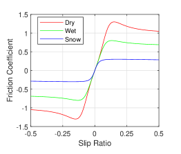
The relationship between the road-tyre friction coefficient and wheel slip is shown in Fig. 3 for both braking and driving cases (i.e., negative and positive slip respectively).

Figure 3: Wheel slip - friction coefficient relationship for positive and negative slips.

III Passive vs Active Learning with Dual Control

An estimator may also be able to quantify the uncertainty of an estimation, e.g. covariance matrix in Kalman filter or particle weights in a Particle filter, when evaluating a state or parameter. Yet no explicit action is taken to reduce this so long as the control reference/objective is achieved. Therefore, in traditional control, the issue of cognitive dissonance, that is, the contradiction between system belief and observation is not addressed when selecting an appropriate control policy. Similarly, the separation principle whereby an optimal controller and an optimal observer are designed separately is often utilized e.g [22]. However, this introduces more instability in the observer which causes issues in the controller when tracking an estimated state. Dual Control for Exploration and Exploitation (DCEE) is well placed in this regard since it actively takes actions to reduce the stress caused by persistent uncertainty of working in unknown environments whilst following an objective (duality) (e.g[23]).

Traditionally, Dual Control [24] was intractable and difficult to achieve real time implementation, while DCEE is not. Furthermore, in practical goal orientated control systems, the reference may not be known, yet only the high level mission is specified. Hence the reference is required to be estimated during the operation of the controller and within an unknown or unfamiliar environment. In this sense, the DCEE approach is more beneficial than Reinforcement Learning that is limited when dealing with changing tasks [25]. DCEE takes this idea of an initially unknown reference into consideration and due to the duality of the method, the uncertainty associated with it is in an exploration/exploitation manner. Furthermore, TVAL makes improvements on the issue of cognitive dissonance by considering both the estimator uncertainty and controller uncertainty when deciding on whether to do active learning or not.

Figure 4: Identification of both current friction coefficient (top) and maximum available friction (bottom) over a varying road surface shown by the change in true maximum friction coefficient (red). Note that the blue curve is the mean value of the estimation, while the green and purple curves show the upper bound and the lower bound of the estimation.

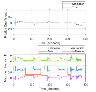
One may argue that an estimator (a particle filter for example) may in fact be able to eventually identify a parameter whilst only requiring the passive stimulus from the driver of a road vehicle e.g. throttle or brake input. However separating the belief update and control action selection does not always perform accurate identification as shown in Fig. 4 where the road surface friction coefficient and parameter D (maximum road friction) of the Magic formula are estimated over a changing road surface. This uses the particle filter and simulation vehicle discussed in the remainder of this paper. The particle filter represents its belief using a distribution of particles and associated weights that are updated upon receiving a new measurement. The estimation is therefore the weighted mean of the distribution. We can see that the current friction coefficient is estimated well after a short identification period. However parameter $D$, vital in the emergency braking procedure, is not estimated well due to the fact that the vehicle hasn’t adequately explored the state space.

In this example the stress (or uncertainty) of the observer is shown using the range of the particle distribution (green and purple lines) that never improves toward the expected value shown in blue. Convergence of the particles is expected if the estimator is behaving as intended. In this regard, given the uncertainty is very high, no control policy could be confidently derived from it. Furthermore, the estimation frequently transitions between estimation periods that are stable and unstable. Thus, the motivation for actively choosing a control policy that explores the agent state and parameter space is necessary, taking into account the belief, hence an active learning approach, such as DCEE is necessary.

IV Torque Vectoring for Active Learning

Identification of the peak friction coefficient is achievable when using the exploration-exploitation nature of DCEE e.g. as part of the Anti-lock Brake System (ABS) in [2]. However, when planning if emergency braking is required, both the peak and current friction coefficients must be known a-priori. Periodically applying ABS is not possible since extreme braking is not acceptable as part of normal, driver controlled, driving. Thus we present a method using the DCEE framework [23] to achieve this. The control scheme can be divided into two parts, firstly an observer which updates the belief and performs the identification of the partially observable states and parameters. This is briefly discussed in this section although full description can be found in [2]. Secondly the whole vehicle torque vectoring for active learning (TVAL) is introduced that updates the action in an exploration-exploitation fashion whilst following the driver’s reference.

IV-A Torque Vectoring Control Strategy

This work assumes that states and parameters of the Magic Formula tyre model (8) are unknown and should be estimated in an online manner. A Regularized Particle Filter observer is used to generate a belief in the augmented state given sequential sensor observations of the vehicle states. The system dynamics is described in (10) using the vehicle state $\mathbf{x}$ that are the vehicle body velocity $v$ and the front and rear axle wheel speeds $\omega_{f,r}$ i.e. $\mathbf{x}=\left[v,\omega_{f},\omega_{r}\right]^{T}$. In addition, $\mathbf{u}$ represents the control input for each wheel, i.e., brake or throttle, while $\mathbf{\Theta}=\left[B,C,D,E\right]^{T}$ denotes the parameters of the tyre model. No lateral motion of the vehicle is assumed and hence only braking or driving is considered.

$$\mathbf{x}_{k} =f\left(\mathbf{x}_{k-1},{\mathbf{u}}_{k-1},\mathbf{\Theta}_{k-1}\right)$$ (10)

$$\mathbf{y}_{k} =\mathbf{x}_{k}+\mathbf{V}_{k}$$

Remark 1

During normal driving, lateral vehicular accelerations are higher than forward accelerations hence the state space can be explored more using just a passive input. Therefore the longitudinal only motion that we consider here presents a more challenging scenario to perform identification.

The measurements of the vehicle states, $\mathbf{y}$, have independent additive Gaussian noise, $\mathbf{V}$. The augmented state matrix is defined as the states of the vehicle, i.e., body and wheel speeds and all four Magic formula parameters:

$$\mathbf{\chi}_{k}=\begin{bmatrix}\mathbf{x}_{k}\\ \mathbf{\Theta}_{k}\end{bmatrix}=\begin{bmatrix}f\left(\mathbf{x}_{k-1},\mathbf{u}_{k-1},\mathbf{\Theta}_{k-1}\right)\\ \mathbf{\Theta}_{k-1}\end{bmatrix}$$ (11)

A simplified discrete time 3DOF, longitudinal model is used here for estimation and prediction where we account for front and rear wheels along with the normal load that we assume to be known a-priori. Since there is no lateral load transfer, the right and left wheels on each axle produce the same tyre force. Using the Forward Euler Method, the predicted ego body velocity is found as:

$${v}_{k}=\frac{2\Delta t}{m}\left[{F}_{k-1,f}+{F}_{k-1,l}\right]+{v}_{k-1}$$ (12)

Similarly each wheel speed can be calculated by

$${\omega}_{k,\{f,l\}}=\frac{\Delta t}{I_{w}}\left[u_{k-1,\{f,l\}}-{F}_{k-1,\{f,l\}}R\right]+{\omega}_{k-1,\{f,l\}}$$ (13)

where $\Delta t$ is the sampling period and we assume that the wheel inertia is the same between each wheel. The parameters are assumed to be piece-wise constants, i.e., $\mathbf{\Theta}_{k}=\mathbf{\Theta}_{k-1}$. Then using (7)-(9) the predicted tyre force can be found using the vertical load on the tyre.

Using the Particle filter formulation from [2], the augmented state matrix is estimated at every discrete time step $k$ using $i$ number of particles:

$$\bar{\chi}_{k}=\mathbb{E}\left[\mathbf{\chi}_{k}\right]=\sum_{i=1}^{n_{i}}W_{k}^{i}\mathbf{\chi}_{k}^{i}$$ (14)

In this work we use $10,000$ particles although this may be tuned to trade-off between computational speed and accuracy.

The DCEE framework [23] acknowledges that a future action will change the future observation. Hence using the aforementioned system model one may predict the observation of the vehicle’s tyre forces. For efficiency, we hypothesise over a finite set of discrete actions $\mathcal{T}$ and allows for us to incorporate the rate limitations of the actuator dynamics into the control policy. In this case we use the following action set; $\mathcal{T}\in\left[0,\pm 1,\pm 10,\pm 100\right]$. The use of electrified powertrains allows the application of torque to be achieved much faster and more accurately [26] than traditional vehicles. Furthermore the use of individual motors for each wheel is more effective than active differentials which is traditionally the case [27]. This makes the use of torque vectoring and the selection of our actions realistic and realisable for improving the stability of vehicles.

TVAL aims to drive the vehicle to explore the epistemic uncertainty of the maximum tyre at one axle, then using the wheels at the other axle to provide a reactive force and achieve the acceleration demand from the driver. The objective for the vehicle can be expressed as:

$$ma_{ref}=\sum^{4}_{j=1}F_{xj}$$ (15)

where $a_{ref}$ is the driver acceleration demand from the or brake and throttle inputs. Thus, this work aims to provide an autonomous means to explore the road surface without interfering with the driver. However our goal orientated approach is to explore the maximum limits of adhesion thus we do not use (15) as the subject of our control scheme. Instead, we aim to find a policy that drives the rear wheel towards the maximum tyre force that is unknown but can be predicted. Additionally, due to the dual nature of this controller, the uncertainty of the tyre being at the maximum tyre force is also evaluated in the same optimization framework. We therefore reduce the cognitive dissonance of the system in an online manner by giving action to the perception and reducing uncertainty.

The optimization routine is outlined in (16) where the objective is to track the predicted future tyre force at the rear wheel, $F_{k+1\mid k,r}^{*}$. This is estimated using the posterior estimate of the maximum friction coefficient (that is parameter $D$ from the Magic Formula tyre model). The predicted friction coefficient ${\mu}_{k+1\mid k,r}$ can then be used similarly with the vertical tyre load to find the predicted tyre force $F_{k+1\mid k,r}$. Since we use predicted observations to inform the likelihood of predicted states, predicted tyre force measurements are generated using the aforementioned system model and the future expected state found using (14).

$$\min_{\mathbf{U}_{tv,k}}J\left(\mathbf{U}_{tv,k}\right)=\min_{\mathbf{U}_{tv,k}}\mathbb{E}_{\mathbf{\Theta}_{k}}\left[\mathbb{E}_{y_{k+1|k}}\left[\big{|}F_{k+1\mid k,r}-F_{k+1\mid k,r}^{*}\big{|}\mid\bar{\mathbf{\chi}}_{k},\mathbf{y}_{k}\right]\right]$$ (16a)

Subject to:

DCEE Wheel

$${F}_{k+1\mid k,f} ={\mu}_{k+1\mid k,f}F_{k+1\mid k,fz}$$ (16b)

$${F}_{k+1\mid k,f}^{*} ={D}_{k+1\mid k}F_{k+1\mid k,fz}$$ (16c)

$$F_{k+1\mid k,fz} =F_{k,fz}$$ (16d)

$${\Theta}_{k+1\mid k} ={\Theta}_{k}$$ (16e)

$${u}_{k,d} ={u}_{k-1,d}+{\tau}_{k}$$ (16f)

$${\tau}_{k} \in\mathcal{T}$$ (16g)

Reactive Wheel

$${F}_{k+1\mid k,r} ={\mu}_{k+1\mid k,r}F_{k+1\mid k,rz}$$ (16h)

$$\mathbf{U}_{tv,k} =\left[u_{k,a},u_{k,d}\right]$$ (16i)

Driver Intention

$$F_{k,ref} =a_{k,ref}F_{k,fz}$$ (16j)

$$F_{k+1\mid k,f}\left(u_{f}\right) =F_{k,ref}-{F}_{k+1\mid k,r}\left(u_{k,r}\right)$$ (16k)

Note that we make the same assumptions as we did for the observer that the parameters are piecewise constants. Furthermore we also assume that the vertical tyre load doesn’t change over the one step prediction.

IV-B Sensor Driven Resampling

Perpetuated operation of the observer, as is the case in real world systems, leads to belief perseverance in the estimated state which is detrimental to sudden changes in the operating point. Similar concepts include perceptual narrowing in neuroscience disciplines. In other words, the believed uncertainty in the identification of the state estimation becomes exceptionally low when the observer has generated a very high belief, and the estimation space converges to a very small region. Using resampling based upon uncertainties therefore becomes degenerate if the road surface does not change for an extended period and the passive stimulus from the driver is small. This behaviour is clear by looking at Fig. 3 since at low slip ratios it is challenging to distinguish between which road surface the vehicle is travelling on. This phenomenon led to the Retrogressive resampling procedure, introduced in previous work [2]. Different to previous Retrogressive resampling applications, this work requires the observer to provide estimations over significantly longer periods of time. Compared to [2] that demonstrated short estimation period (i.e., less than $4s$) over a single road surface change, this work however acknowledges that normal journey times are significantly longer and over different road surfaces.

The resampling procedure is required to avoid immediate degeneracy upon changing to different road surfaces. Motivated by the idea of using commonly available vehicular sensors, we use the rain and light sensor found on most passenger vehicles. This sensor, typically located behind the rear-view mirror, is used as a driver assistance system to activate or adjust the frequency of the windscreen wiper, leaving the driver to focus on the road. Although these group of sensors may be viewed as rudimentary, other sensors such as humidity or temperature sensors may also be used to recognize a change in road surface however sophisticated vision based systems have also found practical application e.g. [28]. We therefore may correlate the detection from the rain/light sensor to a changing road surface and the accumulation of rain or snow on the road surface.

Remark 2

Since the estimation time of the augmented state is very quick, the sensitivity on the controller to frequently changing environments is not significant. However this of course does come at the expense of any existing belief in the tyre and environment which must be re-identified at the cost of vehicle battery power.

We can therefore modify the Retrogressive resampling algorithm to reset the parameter estimation to their initial, diverse state. This is shown in Algorithm 1.

Algorithm 1 Retrogressive Resampling

Input: ${\mathbf{x}}^{i}_{k},\mathbf{\Theta}_{0}^{i},\mathbf{\Theta}_{k}^{i},w^{i}_{0},w_{k}^{i},\rho_{k},\rho_{k-1}$
    Output: ${\mathbf{x}}^{i}_{k},\mathbf{\Theta}_{k}^{i},w_{k}^{i}$

1:  if $\rho_{k}\neq\rho_{k-1}$ then

2:     $\mathbf{\Theta}_{k}^{i}\leftarrow\mathbf{\Theta}_{0}^{i}$

3:     ${\mathbf{x}}_{k}^{i}\leftarrow\mathbf{x}^{i}_{k}$

4:     ${w}_{k}^{i}\leftarrow w^{i}_{0}$

5:  else

6:     $\mathbf{\Theta}_{k}^{i}\leftarrow\mathbf{\Theta}_{k}^{i}$

7:     ${\mathbf{x}}_{k}^{i}\leftarrow\mathbf{x}^{i}_{k}$

8:     ${w}_{k}^{i}\leftarrow w^{i}_{k}$

9:  end if

V Torque Vectoring Demand Regulation

Continuous active learning is inefficient, unnecessary, and potentially unsafe. Here the availability, energy consumption and safety of performing TVAL is considered. Additionally, a smooth integration scheme between active and passive (driver only) is required.

V-A Energy Consumption

Torque vectoring requires significant energy since it requires energy to perform additional tasks above those required to drive or brake the vehicle. Hence management of resource consumption must be addressed particularly since consumers place high weighting on battery range. One method to quantify this would be to compute the work done by each wheel and find the energy consumption above that required by the driver then defining a minimization policy. However, this is not a goal orientated approach to resource management, rather solely a resource management approach which is unaware of the identification goal of the controller. If the system can generate a belief of high confidence in the friction coefficient and associated parameters, then it does not need to continuously operate since we may not be able to improve the estimation further. A comparison of different activation thresholds based on measurement and estimation error, $v_{error}$ (pink line), sensor accuracy $S^{2}_{y,k}$ and estimation uncertainty $S^{2}_{k}$ (green line), and estimation and prediction uncertainty $S^{2}_{k+1\mid k}$ (blue line) is presented in Fig. 5 while estimating parameter D over $400s$ using the Extra-Urban Drive Cycle (EUDC). It is clear to observe that the most effective way to activate TVAL is to compare the measurement uncertainty with the predicted one calculated using

$$S_{k+1\mid k}^{2}=Var\left(\bar{F}_{k+1\mid k}^{*}\right)$$ (17)

If the uncertainty in the maximum force prediction becomes less than that in the estimated maximum force, then the system is required to improve the estimation through the exploration and exploitation effort. This can be achieved using the covariances $S^{2}$ and the following relationship:

$$\tau_{p}=S^{2}_{k}>S^{2}_{k+1\mid k}$$ (18)

which when satisfied, requires the DCEE to be actived in learning the new system states and thus improving the estimate of augmented state matrix.

Figure 5: Comparison of different TVAL activation strategies. Results using sensor $S_{y,k}^{2}$ and estimation $S_{k}^{2}$ uncertainty are shown in green, error between sensor measurement and estimation is compared against a threshold of $1$ in pink and the result using estimation and prediction uncertainty is shown in blue.

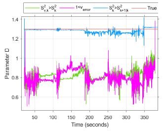
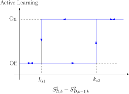
However, this can result in unnecessary chattering around the threshold that does not improve the estimation. Hence although a reduction in the uncertainty caused by a selected action may temporarily reduce the uncertainty, it may not have reached a steady state. Therefore we employ a Hysteresis switch to manage the activation of the TVAL scheme, as shown in Fig. 6. Here the reset point $k_{s1}$ determines when TVAL is no longer required and driver only operation is requested. Then a switching point $k_{s2}$ indicates the threshold where the system is suitably uncertain or stressed and hence the TVAL is activated.

Figure 6: Energy saving Hysteresis switch design. The error between uncertainties on predicted and estimated maximum tyre forces is used to switch between On and Off active learning states. Two gains, $k_{s1}$ and $k_{s2}$ are used to govern the behaviour.

V-B Vehicle Stability

Vehicle understeer or oversteer is the phenomena of a vehicle not following a curved path from a constant steer input. In the case of understeer, the vehicle turns less than the reference input and conversely an oversteering vehicle rotates more. In our longitudinal only problem, this remains an important consideration since the high forces experienced by the tyre during torque vectoring reduces the responsiveness to steering inputs. This instability can be estimated using the understeer gradient and is dependent on the cornering stiffness of the front (and rear) tyres $C_{\alpha f}$ (and $C_{\alpha r}$) as

$$K_{us}=\left(\frac{F_{zf0}}{C_{\alpha f}}-\frac{F_{zr0}}{C_{\alpha r}}\right)$$ (19)

where $F_{zf0}$ (and $F_{zr0}$) represents the static load at the front (and rear) axle [29]. $K_{us}$ represents the understeer gradient. If $k_{us}>0$ then the vehicle is said to be understeering and if $k_{us}<0$, then the vehicle is oversteering. Although both phenomena are undesirable, oversteer is unstable and considered to have greater risks since advanced driver behaviours are required to regain control. Conversely, escaping understeer is achieved by reducing the vehicle velocity. The critical speed $v_{crit}$, used to determine at what speed oversteer occurs, is calculated by

$$v_{crit}=\sqrt{\frac{gl}{\mid K_{us}\mid}},$$ (20)

where $g$ is the gravity constant. This allows us to compare current or predicted ego vehicle velocities to the critical velocity and determine instability in an online fashion. According to [29] we can find the individual cornering stiffness as a function of the friction coefficient $\mu_{k}$, vertical $F_{k,z}$ and longitudinal $F_{k,x}$ loads for each wheel:

$$C_{k,\alpha}\left(\mu_{k},F_{k,z},F_{k,x}\right)=\varphi_{k,x\alpha}\left[C_{k,\alpha}\left(F_{k,z}\right)-\frac{1}{2}\mu_{k}F_{k,z}\right]+\frac{1}{2}\left(\mu_{k}F_{k,z}-F_{k,x}\right)$$ (21)

where

$$\varphi_{k,x\alpha}=\left[1-\left(\frac{F_{k,x}}{\mu_{k}F_{k,z}}\right)^{n}\right]^{1/n}$$ (22)

using $n$ between $2-8$. Additionally, the cornering coefficient as a function of the vertical load (only) is found using the coefficients of the Magic Formula $c_{1}$ and $c_{2}$ and nominal load $F_{z0}$:

$$C_{k,F\alpha}=c_{1}c_{2}F_{zo}\sin\left\{2\arctan\left(\frac{F_{k,z}}{c_{2}F_{zo}}\right)\right\}$$ (23)

Therefore to enforce the stability, the following constraint should be applied:

$$\tau_{k,s}=v_{k+1\mid k}<v_{k+1\mid k,crit}$$ (24)

Note that we consider predicting if the vehicle has the potential to oversteer. Since torque vectoring places additional demand on the vehicle, it is important to recognize that the drivers input can be unpredictable. Hence the above constraint is necessary for (partially) autonomous systems such as automated driving.

V-C Tyre Force Availability

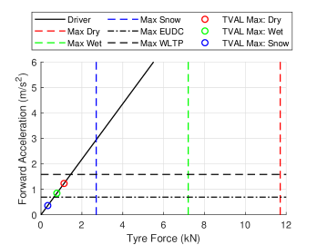
If the maximum friction coefficient is known, or in this case estimated, the maximum permissible acceleration of the vehicle is known across any road surface. Since this information is available to our controller, we can determine whether the acceleration request from the driver is achievable whilst also performing identification of the augmented state vector. This idea is shown in Fig. 7 where the acceleration and deceleration limits are shown when performing active learning (coloured circles) and when the vehicle is operating without (dashed) i.e. driver only. This limitation is found as a result of the weight distribution of the vehicle. If the vehicle were to be excessively front loaded i.e. all the vehicles weight were over the front axle, then a much greater acceleration would be possible. Since their would be a smaller maximum tyre force at the rear required to explored (for the purposes of actively learning the road surface) and therefore much more tyre force at the front to equal this and also achieve the acceleration request from the driver.

In Fig. 7 the solid black line shows the tyre force required for just achieving the desired acceleration. We can see that TVAL comes at the expense of not being able to achieve the driver’s request. For example, if the driver wanted to accelerate at $1m/s^{2}$, TVAL would only be achievable on a dry road surface. Yet without TVAL, the vehicle could achieve this on any road surface discussed here as shown by the coloured dashed lines. While decelerating, only the friction limits of the road surface constrain the controller.

Remark 3

This further highlights the need for active learning, since only at the extreme acceleration of $\pm 11.7m/s^{2}$ would the driver exploit the full friction of the dry road.

One may argue that TVAL is too limited to work within the operation of normal driving behaviours. This however is not the case when considering drive cycle descriptions of human behaviour. In the case of the maximum accelerations found in the EUDC (demonstrated in Section VI) and the WLTP (Worldwide Harmonised Light Vehicles Test Protocol), the vast majority of driving allows for the use of TVAL, depending on the surface. The peak acceleration found in each of these cycles is shown on Fig 7 as dash-dotted and dashed lines repectively.

Hence a constraint (7) is chosen to govern the activation and deactivation considering the maximum availability of tyre force using the estimated friction coefficients $\bar{F}^{*}_{fx}$.

$$\tau_{a,k}=\frac{m}{2}a_{ref,k}\geq\bar{F}^{*}_{fx,k}+\bar{F}^{*}_{rx,k}$$ (25)

Figure 7: Available tyre force on different road surfaces (using road surface data in Fig. 3). Maximum acceleration when using TVAL (coloured circle) and the required demand when just the driver is in control (black line).

V-D Input Management

Figure 8: Activation modulation scheme.

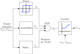
The request for active learning is simply if all Eqs. (18), (24) and (25) are satisfied. Switching on or off between active learning and driver controls, after the tyre model has been identified and TVAL constraints satisfied is not a suitable strategy since the sudden deactivation could lead to front wheel torque inputs to rapidly decrease or increase. This leads to an increase in acceleration and thus greater discomfort on the driver.

Remark 4

This highlights the challenge associated with higher level autonomous driving such as SAE level 3 autonomous driving [30]. Changing between driver and autonomous control cannot be as straightforward as on or off and must be managed carefully to ensure smooth, controllable handover.

To mitigate this and control the learning activation rate, a linear mapping between the two controllers is now presented, that is, between the driver and our torque vectoring scheme. This is shown in (26) using the wheel inputs as calculated by the torque vectoring controller, $\mathbf{U}_{tv,k}$, and the driver input $\mathbf{U}_{driver,k}$:

$$\mathbf{U}_{veh,k}=w_{1,k}\mathbf{U}_{tv,k}+\left(1-w_{1,k}\right)\mathbf{U}_{driver,k}$$ (26)

Using weight $w_{1,k}$ to moderate the transition between the two systems. This rejects small changes in the road surface from causing TVAL to become active. It additionally prevents chattering from the combined effort of each constraint, forcing a pause between torque vectoring identification effort. Simply, if the request for active learning ($\tau_{r,k}==1$) is satisfied most of the time, then torque vectoring should become activated. Conversely, if there is no demand for active learning i.e. $\tau_{r,k}==0$ is satisfied most of the time, then only the drivers input should be passed to the vehicle. This request counter relationship, $f_{k}$ is captured using equation (27):

$$f_{k}=f_{k-1}+\left(\tau_{r,k}==1\right)-\left(\tau_{r,k}==0\right).$$ (27)

To ensure that the weighting is bound between $0$ and $1$, the request counter function is bounded as well:

$$f_{k}=\begin{dcases}0,&f_{k}=0\\ f_{k},&0<f_{k}<\Delta P\\ \Delta P,&f_{k}\geq\Delta P\end{dcases}$$ (28)

Finally, the weighting function can be found using the request gradient, and $\Delta P$ is tuneable depending on the desired transition period. The tuning methodology follows that one should select $\Delta P$ to be the transition time between either inputs which may be in the order of a few seconds. Finally, the time dependant weighting can be found as:

$$w_{1,k}=\frac{f_{k}}{\Delta P}$$ (29)

The modulation of the active learning is shown in Fig. 8 that is a combination of all three constraints which drives the application of the driver and torque vectoring inputs (26) to the vehicle.

VI Drive Cycle Performance

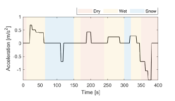
In lieu of comparative studies, we demonstrate our controller using a drive cycle and show that the energy and power consumption is significantly reduced whilst maintaining an accurate estimate of both current friction and maximum friction. A changing road surface (see Fig. 9) is also tested to further show the ability to maintain a stable estimation and adapt to changes in the environment. In this scenario we assume that a GPS and wheel speed senors are used with zero bias Gaussian noise i.e. $\mathbf{V}_{k}\sim\mathcal{N}\left(\left[0,0,0\right]^{T},diag\left(0.2,0.5,0.5\right)\right)$. We are required to use a driver model to track the reference acceleration profile when active learning is not engaged and respond to changes in acceleration. This driver model is formed of two parts, a drive cycle that models the intended reference over the entire simulation and a PI controller that responds to the tracking error. This model is shown in Fig. 1. The EUDC was chosen over the most recent WLTP since it has simpler behaviours thus as to not excessively passively perturb the system. This in turn requires our controller to actively explore the system more and hence shows a more challenging scenario. The associated proportional and integral gains are $k_{P}=0.01$ and $k_{I}=15$ respectively. The Particle Filter is initialized with the properties in Table I.

Figure 9: The EUDC acceleration profile across changing road conditions for dry (red), wet (yellow) and snow (blue) road surfaces.

TABLE I: Particle Filter range of initial values.

$v_{0}$	$w_{f0}$	$w_{r0}$	$B_{0}$
$\left[0.5,4.5\right]$	$\left[2.0,9.0\right]$	$\left[2.0,9.0\right]$	$\left[4.0,21\right]$
$C_{0}$	$D_{0}$	$E_{0}$
$\left[1.3,1.7\right]$	$\left[0.2,1.6\right]$	$\left[2.0,-12\right]$

VI-A Controller Stability

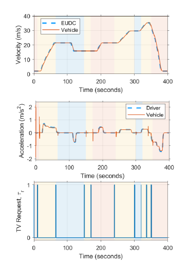
Whilst the standard EUDC model has prolonged initial and final periods of stationary behaviour, we offset the velocity and initialize the vehicle starting at $2m/s$. This is beneficial for demonstration since TVAL is not required when the vehicle is stationary. It is assumed that the vehicle is running on an unknown road surface thus must actively probe the environment through TVAL to reduce the uncertainty in its belief of the friction. Large uncertainty in beliefs of the augmented state is represented by a wide initial distribution of particles in our particle filter setting. In Fig. 10, TVAL is shown to activate immediately and follow a constant velocity on the initially dry road surface. Overall the acceleration of the ego vehicle tracks that of the driver with only transient increases either upon traversing a new surface or initially in the scenario where ego state estimates are converging. Here the torque vectoring is exploring the road surface and performing those actions to minimize the exploration-exploitation objective, which in turn, improve the ability to follow the reference. Although the acceleration tracking error experiences temporary tracking error, this does not impact the velocity of the overall vehicle or cause a deviation of from the original EUDC reference. That is also shown in Fig. 10. Compared to similar works [18] that operate for small slip angles, our method performs better since in this work an acceleration error of $0.7m/s^{2}$ is reported. Furthermore, as is shown in Fig. 11, the tyre forces are higher on a dry road and if the estimation accuracy is poorer, the vehicle can quickly generate higher accelerations. Additionally the affect of our input management mapping is clear since at $320s$ where the surface changes from snow to wet and a brief request for TVAL as a result. Therefore due to the unavailability of the tyre force, torque vectoring and identification of the road surface cannot be achieved. However because we limit the rate at which TVAL can begin active learning, the availability constraint becomes violated shortly after and hence doesn’t fully engage which minimizes any impact from the increase in torque to the vehicle.

Figure 10: Vehicle velocity (top) compared with the EUDC (desired) reference, vehicle acceleration (middle) against the drivers acceleration request and TVAL request, $\tau_{r}$ (bottom).

Figure 11: Front and rear vehicle tyre forces with the activation weight $w_{1,k}$ overlaid as a colormap where dark blue represents full active learning input to the vehicle and white shows driver only. The maximum tyre forces for front and rear are also shown.

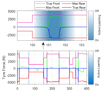
The front and rear tyre forces rise uniformly upon activation of TVAL as shown in Fig. 11 with the active learning weighting shown as a colormap. Immediately upon changing road surface, the maximum possible tyre force increases and the TVAL request begins to transition from driver to active learning. Here the tyre force slowly builds until shortly after the initial activation. The delay transition gradient is set to $\Delta P=1$ where it can be seen that after this period, the rear tyre force reaches the maximum. In the example shown in Fig. 11, TVAL takes only $0.5s$ to identify the Magic formula parameters where the complete active learning cycle (driver to driver) lasts approximately 2.5s. Noting that of this, $2.0s$ is tunable depending on rate of transition between torque vectoring and driver inputs.

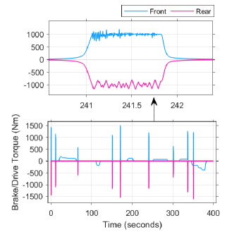
This steady transition is evident in the vehicle torque inputs shown in Fig. 12 and both front and rear reach a steady state for the duration of the active learning, with smooth transition leading up to and back to the driver. Although the front wheel shows a constant torque input the rear, which is performing the exploration-exploitation action has more steady state oscillation. This is due to the exploration nature of the DCEE controller. Despite that there are larger oscillations, this does not have a significant impact on the tyre force since at this maximum, changes in slip (driven by the changes in the control input) do not have as significant impact compared to lower (elastic) slip ratios. This is clear from the slip-$\mu$ relationship in Fig. 3.

Figure 12: Front and rear wheel control input during changing road conditions.

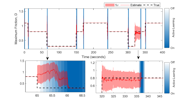
VI-B Friction Estimation and Tyre Force Uncertainty

The change of the maximum road surface friction coefficient may be considered extreme, changing 9 times in 400s however this exhibits the control systems ability to identify a range of conditions and hold its belief. The estimation of parameter D is shown in Fig. 13. On low friction (snow) surfaces the maxima is less well defined that makes it the most challenging of all road surfaces selected here. At $65s$ the estimation stabilizes to $D=0.284$ giving an error of $0.016$ (i.e. $5\%$) before switching to the driver since it believes it has generated a good belief in the augmented state. Then at $320s$ TVAL activates for a very short period and doesn’t reduce the uncertainty enough which can be noticed from the fluctuating estimation until the forward acceleration request from the driver reduces to where TVAL becomes available. This $320-345s$ (Fig. 13) period shows how the estimated maximum friction and uncertainty (pink) persists until TVAL reduces the estimation error and shrinking the confidence interval before handing over to the driver in a short period of time.

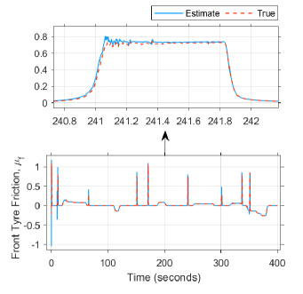
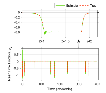
The estimated friction coefficient, shown in Fig. 14 and Fig. 15 and is estimated well throughout the scenario, even while the driver is in full control. Performance suffers very slightly when the friction reaches the maximum on a dry road however the observer quickly converges back to the ground truth. On wet and snow surfaces, the particle filter has no issue in estimating the current friction.

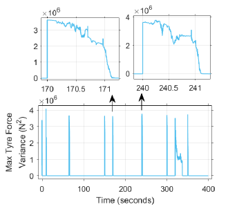
Since this work uses a dual approach, we consider both the reference tracking and performance in reducing the uncertainty of the system. In Fig. 16 the estimation uncertainty in the maximum tyre force over the scenario is shown and highlights how the uncertainty decreases as the active learning (TVAL) is used. In all cases where TVAL is fully active, the uncertainty decreases. One can see that during the first second ($\Delta_{p}$) the uncertainty decrease but at a slow oscilitory manner. However once TVAL becomes fully engaged (after $1s$) the uncertainty drastically reduces. Notable the steady state uncertainty is reduced more than $99.998\%$ of the original value, yielding $6.8N$ standard deviation on the road surface staring at $170s$.

Figure 13: Estimation of the maximum road surface friction (parameter D) over changing surfaces (black dash), shown with the estimation uncertainty as shaded pink area (1 standard deviation) and active learning activation weight shown in blue. Note that the time taken to reach active learning fully on i.e.$w_{1,k}=1$, is tuneable where here this is set to 1 second i.e.$\Delta P=1$.

Figure 14: Rear tyre friction coefficient estimation from the Particle Filter.

Figure 15: Front tyre friction coefficient estimation from the Particle Filter.

Figure 16: Maximum tyre force uncertainty found from the Particle Filter estimation.

VI-C Safety and Tyre Wear

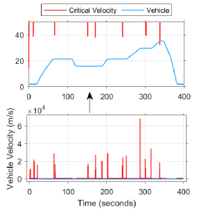
TVAL was predicted to exceed the critical velocity at high velocities on wet road surfaces which is to be expected given the limited available tyre force. The vehicle is travelling at $35.3m/s$ ($79mph$) during this stage which is outside normal driving for most vehicles however shows the ability of our method to operate at high speeds and low speeds ($4mph$). This part of the scenario is also made more challenging since the driver is accelerating here. Therefore the simulation results show that TVAL was able to prevent the scenario that put the vehicle into a state where oversteer would have occurred if there were to be a lateral disturbance. The estimation of the critical velocity and ego vehicle velocities are shown in Fig. 17.

Figure 17: Critical velocity used to activate TVAL.

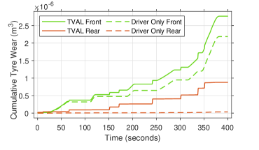
Tyre wear is increased when performing tyre excitation and discussed here using Archard’s wear model [31]. Despite this, since TVAL considers the deactivation of the active learning, it is only engaged for as long as is necessary to learn the friction properties. Therefore the period of maximum tyre wear is typically limited to less than $0.6s$ across the scenario where active learning is fully engaged. Furthermore, high friction surfaces generate the largest wear (higher tyre forces) yet this is where the best braking performance for AEB can be achieved. Hence future work may consider that when high wear is experienced, active learning may be relaxed to preserve the tyres.

Figure 18: Tyre wear comparison between driver only and our (TVAL) method using Archard’s tyre wear method. Note that during driver only mode, the vehicle is front wheel drive only compared to TVAL that is all wheel drive.

VI-D Power and Energy Consumption

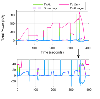
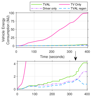
As with any torque vectoring controller, additional energy is expended to achieve additional control tasks. The power and energy consumption is presented in Fig. 19 and Fig. 20 respectively. A $96\%$ reduction in the energy consumption is made when compared to applying torque vectoring without regulation (TVAL) i.e. torque vectoring only. Additionally, TVAL requires on average $1.5$ times the energy that normal driving requires. One should consider that the vehicle is very unlikely to experience such challenging weather conditions, changing 9 times in 400s however this scenario is chosen to show the robustness of our method. Importantly, regenerative braking, which is the recovery of energy used in braking, can be applied here (as is the case for most electric vehicles) and is also included within Fig. 19 and Fig. 20. Typically one may expect the efficiency of regenerative braking under heavy braking to be $0.7$ which significantly offsets the active learning effort [32]. This is particularly noticeable in Fig. 20 where it can be seen that assuming this recovery efficiency, our method requires less energy than normal driving with non-regenerative braking. Hence we argue that TVAL can effectively be used without causing excessive additional range anxiety to consumers, particularly given the benefit TVAL brings to active safety.

Further shown in Fig. 19 is the power consumption that increases for very short periods of time when doing the exploration/exploitation action. A summary of the average power consumption is shown in Table II.

Figure 19: Vehicle power consumption shown for our scheme (TVAL), TVAL with regenerative braking, full torque vectoring for the entire scenario i.e. always torque vectoring (TV Only) and driver only (no torque vectoring). The full torque vectoring (blue) is computed using theoretical maximum tyre forces since full torque vectoring isn’t practically achievable in this scenario which explains the transient overshoot of TVAL over the torque vectoring.

Figure 20: Cumulative power consumption shown for our scheme (TVAL), TVAL with regenerative braking, full torque vectoring for the entire scenario i.e. always torque vectoring (TV Only) and driver only (no torque vectoring).

TABLE II: Mean power consumption.

Method	Average Power ($kW$)
Driver Only	6.84
TV	247
TVAL	10.4
TVAL with Regenerative Braking	1.93

VII Conclusion

TVAL is capable at identifying some of the major components required for emergency braking features such as AEB. Knowing the current friction, peak friction coefficient and tyre model, the decision-making process for extreme braking manoeuvres is significantly improved. Utilizing regenerative braking, we show that our work does this with less energy consumption than non-regenerative normal driving. We look in future work to event driven TVAL including alerting the driver and delivering a holistic AEB system using this approach. This work, although applied to an Automotive use case, is applicable to the broader field of robotics. TVAL can be used where the ego vehicle reference is known and the broad behaviour of the vehicle that excites the identification of a given parameter, is also known. In this case, braking or accelerating toward the friction limits. An example for further investigation includes exploiting upcoming drive-by-wire systems that are due to be introduced into mainstream production and identifying lateral tyre dynamics.

References

- [1] “Automatic Emergency Braking Performance in the Context of Common Crash Scenarios,” American Automobile Association, Tech. Rep., Sep 2022. [Online]. Available: https://newsroom.aaa.com/page/8/?aaa_asset_type=post&s#038;s
- [2] B. Sullivan, J. Jiang, G. Mavros, and W.-H. Chen, “An exploration-exploitation approach to anti-lock brake systems,” 2023.
- [3] V. Mazzilli, D. Ivone, S. De Pinto, L. Pascali, M. Contrino, G. Tarquinio, P. Gruber, and A. Sorniotti, “On the benefit of smart tyre technology on vehicle state estimation,” Vehicle System Dynamics, pp. 1–26, oct 2021.
- [4] J. Casselgren, S. Rosendahl, and J. Eliasson, “Road surface information system,” in 16th SIRWEC conference, no. May, 2012, pp. 23–25.
- [5] L. Svensson and M. Torngren, “Fusion of Heterogeneous Friction Estimates for Traction Adaptive Motion Planning and Control,” IEEE Conference on Intelligent Transportation Systems, Proceedings, ITSC, vol. 2021-Septe, pp. 424–431, 2021.
- [6] T. S, “Testing and understanding of tire–road interaction on wet roads,” Proceedings of the 13th Symposium Reifen und Fahrwerk, 2015.
- [7] L. Cheng, X. Zhang, and J. Shen, “Road surface condition classification using deep learning,” Journal of Visual Communication and Image Representation, vol. 64, p. 102638, oct 2019.
- [8] X. Wang, J. Wang, W. Sun, Y. Wang, F. Xie, and D. Guo, “Development of AEB control strategy for autonomous vehicles on snow-asphalt joint pavement,” International Journal of Crashworthiness, vol. 27, no. 6, pp. 1601–1621, nov 2022.
- [9] F. Gustafsson, “Slip-based tire-road friction estimation,” Automatica, vol. 33, no. 6, pp. 1087–1099, jun 1997.
- [10] K. Yi, K. Hedrick, and S.-C. Lee, “Estimation of Tire-Road Friction Using Observer Based Identifiers,” Vehicle System Dynamics, vol. 31, no. 4, pp. 233–261, 1999.
- [11] R. Rajamani, G. Phanomchoeng, D. Piyabongkarn, and J. Y. Lew, “Algorithms for Real-Time Estimation of Individual Wheel Tire-Road Friction Coefficients,” IEEE/ASME Transactions on Mechatronics, vol. 17, no. 6, pp. 1183–1195, dec 2012.
- [12] L. R. Ray, “Nonlinear Tire Force Estimation and Road Friction Identification: Simulation and Experiments,” Automatica, vol. 4, no. 97, pp. 1819–1833, 1997.
- [13] Z. Zhang, L. Zheng, H. Wu, Z. Zhang, Y. Li, and Y. Liang, “An estimation scheme of road friction coefficient based on novel tyre model and improved SCKF,” Vehicle System Dynamics, vol. 60, no. 8, pp. 2775–2804, aug 2022.
- [14] F. Djeumou, J. Y. M. Goh, U. Topcu, and A. Balachandran, “Autonomous Drifting with 3 Minutes of Data via Learned Tire Models,” in IEEE Conference on Robotics and Automation, 2023, pp. 968–974.
- [15] B. Ma, C. Lv, Y. Liu, M. Zheng, Y. Yang, and X. Ji, “Estimation of Road Adhesion Coefficient Based on Tire Aligning Torque Distribution,” Journal of Dynamic Systems, Measurement, and Control, vol. 140, no. 5, 2018.
- [16] J. Prokeš, A. Albinsson, and L. Laine, “Quantification of excitation required for accurate friction estimation,” IEEE Conference on Intelligent Transportation Systems, pp. 2551–2558, dec 2016.
- [17] A. Albinsson, F. Bruzelius, B. Jacobson, and J. Fredriksson, “Design of tyre force excitation for tyre–road friction estimation,” Vehicle System Dynamics, vol. 55, no. 2, pp. 208–230, feb 2017.
- [18] A. Albinson, F. Bruzelius, and B. Jacobson, “Identification of tyre characteristics using active force excitation,” in The Dynamics of Vehicles on Roads and Tracks. London: CRC Press, mar 2016, pp. 519–528.
- [19] G. Warth, M. Frey, and F. Gauterin, “Design of a central feedforward control of torque vectoring and rear-wheel steering to beneficially use tyre information,” Vehicle System Dynamics, vol. 58, no. 12, pp. 1789–1822, Dec 2020.
- [20] J. C. Dixon, Tires, Suspension and Handling, Second Edition. SAE International, 1996.
- [21] G. Mavros, “A study on the influences of tyre lags and suspension damping on the instantaneous response of a vehicle,” Proceedings of the Institution of Mechanical Engineers, Part D: Journal of Automobile Engineering, vol. 222, no. 4, pp. 485–498, apr 2008.
- [22] Z. Qin, C. Liang, M. Hu, and X. Chen, “A Lateral and Longitudinal Dynamics Control Framework of Autonomous Vehicles Based on Multi-Parameter Joint Estimation,” IEEE TRANSACTIONS ON VEHICULAR TECHNOLOGY, vol. 71, no. 6, p. 5837, 2022.
- [23] W. H. Chen, C. Rhodes, and C. Liu, “Dual Control for Exploitation and Exploration (DCEE) in autonomous search,” Automatica, vol. 133, p. 109851, Nov 2021.
- [24] A. A. Feldbaum, “Dual control theory. i,” Automation Remote Control, vol. 21, no. 9, pp. 1240–1249, 1960.
- [25] W. H. Chen, “Perspective view of autonomous control in unknown environment: Dual control for exploitation and exploration vs reinforcement learning,” Neurocomputing, vol. 497, pp. 50–63, aug 2022.
- [26] M. Heerwan, B. Peeie, H. Ogino, and Y. Oshinoya, “Skid control of a small electric vehicle with two in-wheel motors: simulation model of ABS and regenerative brake control,” International Journal of Crashworthiness, vol. 21, no. 5, pp. 396–406, 2016.
- [27] L. De Novellis, A. Sorniotti, P. Gruber, and A. Pennycott, “Comparison of Feedback Control Techniques for Torque-Vectoring Control of Fully Electric Vehicles,” IEEE Transactions on Vehicular Technology, vol. 63, no. 8, pp. 3612–3623, Oct 2014.
- [28] C. Tian, D. Jin, B. Leng, and L. Xiong, “Reliable Identification of Road Surface Condition Considering Shadow Interference; Reliable Identification of Road Surface Condition Considering Shadow Interference,” 2021 IEEE International Intelligent Transportation Systems Conference (ITSC), 2021.
- [29] H. Pacejka, Tire and Vehicle Dynamics. Elsevier, 2012.
- [30] O.-R. A. D. O. Committee, Taxonomy and Definitions for Terms Related to Driving Automation Systems for On-Road Motor Vehicles, apr 2021.
- [31] J. F. Archard, “Contact and Rubbing of Flat Surfaces,” Journal of Applied Physics, vol. 24, no. 8, pp. 981–988, aug 1953.
- [32] A. Doyle and T. Muneer, “Traction energy and battery performance modelling,” in Electric Vehicles: Prospects and Challenges. Elsevier, 2017, pp. 93–124.