A Noisy Beat is Worth 16 Words: a Tiny Transformer for Low-Power Arrhythmia Classification on Microcontrollers

Abstract

Wearable systems for the long-term monitoring of cardiovascular diseases are becoming widespread and valuable assets in diagnosis and therapy. A promising approach for real-time analysis of the electrocardiographic (ECG) signal and the detection of heart conditions, such as arrhythmia, is represented by the transformer machine learning model. Transformers are powerful models for the classification of time series, although efficient implementation in the wearable domain raises significant design challenges, to combine adequate accuracy and a suitable complexity.

In this work, we present a tiny transformer model for the analysis of the ECG signal, requiring only 6k parameters and reaching 98.97% accuracy in the recognition of the 5 most common arrhythmia classes from the MIT-BIH Arrhythmia database, assessed considering 8-bit integer inference as required for efficient execution on low-power microcontroller-based devices. We explored an augmentation-based training approach for improving the robustness against electrode motion artifacts noise, resulting in a worst-case post-deployment performance assessment of 98.36% accuracy. Suitability for wearable monitoring solutions is finally demonstrated through efficient deployment on the parallel ultra-low-power GAP9 processor, where inference execution requires 4.28ms and 0.09mJ.

I Introduction

According to the World Health Organization, cardiovascular diseases are the first cause of death worldwide [1]. The electrocardiographic (ECG) signal represents the commonly accepted non-invasive diagnostic and monitoring tool for the detection and recognition of anomalies in the functioning of the heart, whose early detection can help reduce their consequences and provide adequate treatment.

It is established that wearable solutions are of great importance for allowing continuous monitoring of chronic conditions while reducing the burden on clinicians and hospital structures [2]. In this context, where the privacy of the data is a relevant concern, near-sensor edge processing represents an increasingly attractive option. Particular benefits would result from continuous monitoring for the detection of arrhythmia, which represents an anomaly of the heartbeat, showing an irregular or abnormal rhythm.

Neural network-based classification has been successfully exploited for arrhythmia recognition, reaching very high accuracy levels exploiting Convolutional Neural Networks (CNNs) [3]. Even better results have been obtained recently with the use of large-size transformers [4, 5], involving a computational workload not suitable for efficient execution on wearable monitoring devices.

In this work, we plan to combine the advantages deriving from the attention mechanism exploited in transformers with actual execution on wearable devices for long-term monitoring. To this aim, we have designed a lightweight transformer architecture that can be executed on microcontrollers, focusing on limited footprint and complexity. Moreover, we have considered motion artifact noise resilience as a main objective within the overall design process, using signals with artifacts to augment the dataset during training.

We start with a review of the state of the art of classification approaches in Section II. In Section III, we provide a general overview of the considered ECG monitoring system and describe its components, focusing on the architecture of the proposed transformer-based classifier. Section III-C summarizes the specifications of the datasets targeted for this study, whereas Section III-D provides the definition of the evaluation metrics considered for the assessment of the results, namely sensitivity and precision. The assessment of the classification performance is presented in Section IV, including in Section IV-C a post-deployment evaluation, considering the impact of noise resulting from electrode movement artifacts and accuracy drop due to data quantization. Finally, we report in Section V the evaluation of the on-hardware performance of the proposed model deployed on the GAP9 low-power multicore microcontroller unit (MCU).

The main contributions of this work can be summarized in the following points:

• we present a tiny transformer model for arrhythmia recognition, reaching accuracy aligned with the state of the art of transformer-based classifiers, with 60$\times$ fewer parameters and 300$\times$ fewer required operations;

• we evaluate the robustness of our proposed classifier considering common issues of real-time execution, resulting from the presence of artifacts and noise in the signal acquisition;

• we provide an efficient implementation on a low-power commercial MCU, resulting in less than 0.09mJ per inference obtained with quantization up to 8-bit precision and parallel execution on 8 cores, thus showing the proposed model is suitable for long-term wearable monitoring.

II Related Work

Work	Year	Classes	Task	Model	Accuracy	Footprint	Inference	Energy	Hardware Target	Noise
							Time	Consumption		Addition
[5]	2019	4	intra-patient	ViT	99.62%	3MB*	365MOPs*1	-	-	✗
[6]	2022	4	intra-patient	ViT	99.3%	-	-	-	Xilinx Alveo	✗
									U50 FPGA
[4]	2022	4	intra-patient	Transformer	99.49%	20MB	70.53MOPs1	-	-	✗
[7]	2022	5	intra-patient	MLP	$>$ 99%	-	30.41MOPs1	-	-	✗
[3]	2022	8	intra-patient	CNN	99.54%	16MB	-	-	-	✗
[8]	2023	4	intra-patient	CNN	99%	2.2MB	-	-	-	✗
[9]	2022	5	intra-patient	CNN	98.89%	96kB	215 ms	0.66 mJ	ARM Cortex-M4	✗
[10]	2023	3	inter-patient	CNN	98.18%	15kB	1ms	-	Cortex-ARMv8	✓
this work	2024	5	intra-patient	ViT 32-bit	99.05%					✗
				ViT 8-bit	98.97%	49kB	4.28ms	0.09mJ	GAP9	✗
				ViT 8-bit	98.36%					✓

• Estimated from paper.

• The paper reports the model complexity in terms of number of required operations. Our proposed model requires the execution of 0.97 MOPs/inference.

TABLE I: State of the art on the MIT-BIH Arrhythmia database.

Table I summarizes the recent works presenting neural network-based models for arrhythmia recognition on the MIT-BIH dataset [11, 12]. For each of the listed works, we report in subsequent columns the publication year, the number of arrhythmia classes considered, the specific task addressed, the classification model, and the test accuracy obtained. The ”Footprint”, ”Inference Time”, and ”Energy consumption” columns summarize the performance evaluated on the target platform, reported in the ”Hardware Target” column. Finally, for each work, we indicate whether the degradation of the classification accuracy in the presence of growing levels of noise has been explored.

As can be noted, classification based on CNNs reaches remarkable results. In [3] the authors present a CNN adapted from the EfficientNet family, focusing on the 8-class arrhythmia recognition task and reaching 99.54% accuracy with around 5.3M parameters. A 1D-CNN exploiting 2M parameters is presented in [8], reporting 99% accuracy in the 4-class recognition problem. As an alternative, the work of [7] presents arrhythmia classification based on a Multi-Layer-Perceptron (MLP) model, scoring a classification accuracy higher than 99.47% for each of the 5 classes considered.

Tiny CNN models have also been exploited for real-time arrhythmia detection on resource-constrained devices. Ref. [9] presents two alternative CNNs for arrhythmia recognition on a commercial low-power microcontroller, reaching up to 98.69% and 98.89% accuracy in the 5-class recognition problem, with 18K and 93K parameters. The efficiency of inference execution was evaluated on the ST Sensortile microcontroller, where it requires 215ms and 0.66mJ. Hybrid models resulting from the combination of the CNN topology with the MLP, such as in [13], or the Long-Short-Term-Memory (LSTM) network, such as in [14], were also considered for binary classification, to distinguish between normal and ventricular, or generally abnormal, heartbeats. The proposed models reach up to 98.5% and 97% accuracy.

We also include as a reference the work of [10], addressing the more challenging inter-patient classification problem, where the classifier is trained and tested on the data from separate sets of patients. The author presents a CNN working on the first derivative of the ECG signal and exploiting matched filters reproducing the different arrhythmia classes within the convolutional layers. The model also exploits the processing of the RR intervals (the distance between consecutive heartbeat peaks in the signal) through a stack of fully connected layers, obtaining 98.18% accuracy with a 15kB memory footprint. Edge deployment on a Raspberry Pi equipped with a Cortex-ARMv8 64-bit System on Chip results in less than 1ms inference time. This work explores the robustness against increasing levels of noise, considering white noise addition up to 3db Signal to Noise Ratio (SNR).

Another relevant contribution to the issue of inter-patient variability is presented in [15], introducing BioAIP, a specialized processor for biological signal processing. Through the use of an adaptive learning engine, it provides the possibility to refine a CNN-based global classification model considering a small subset of patient-specific data, registering up to 7.5% accuracy improvement on tests following the leave-one-patient-out approach, reaching up to 99.16% classification accuracy.

The state of the art for transformer-based classification is established by the work of [5]. The authors presented a Vision Transformer (ViT) consisting of 3 encoding blocks and 4 parallel heads in the attention layer. They obtained 99.62% accuracy, exploiting a denoising and baseline-wandering removal step, and concatenating the information about the RR intervals within the last classification layer. An interesting approach is presented in the work of [4]. The proposed model is applied on 3s-long windows of signal and provides the positioning and classification of the heartbeats occurring during that period, reaching 99.86% heartbeat positioning accuracy, and 99.49% classification accuracy. The best model exploits 5M parameters, but competitive results were obtained with a similar architecture based on 0.75MB of parameters, reaching 99.05% accuracy.

Other relevant examples are represented by the work of [6], reaching 99.3% accuracy on the MIT-BIH dataset, and the transformer architectures presented in [16, 17, 18], which were designed and tested on different datasets, considering multiple-lead acquisition.

To the best of our knowledge, the transformer-based classifiers in the literature have storage and computational requirements non-compatible with efficient deployment on low-power MCUs. To better motivate this statement, we consider as a reference for wearable deployment a typical storage size of 512kB, which is the available space in the L2 memory of microcontroller-based platforms such as GAP8 [19] and BioWolf [20]. The more recent GAP9, which is further described in Section V, embeds a larger storage space, up to 1.5MB in the L2 memory level, which is still not enough for the allocation of the model in [5]. Finally, the authors of [6] describe an FPGA implementation, but the size and complexity of the model, as well as the inference time and energy consumption, are not reported.

In this work, we thus present an efficient transformer architecture, targeting accurate arrhythmia detection on low-power wearable devices, and extending the performance assessment to the typical challenges of real-time wearable operating conditions. As most of the referenced works, with the exception of [10], we refer to the intra-patient classification problem, where each heartbeat in the dataset is considered independently, and randomly assigned to the training, validation, or test set.

III ECG Classifier Design

A typical ECG signal is shown in Figure 1, referring to acquisition from a single electrode. Each heartbeat is defined by a complex wave around a peak (R) in the amplitude, commonly known as the QRS complex. The shape of the wave around the R-peak, and the intervals between consecutive peaks (pre-RR and post-RR intervals), highlighted in the figure, are both meaningful diagnostic elements.

Figure 1: Typical ECG signal. Highlighted is the considered window around a single heartbeat, the R peak position and the definition considered in the following for pre- and post- RR intervals.

Figure 2 describes a general overview of the real-time monitoring system that would be executed on a wearable device. The input to the system is represented by the continuous ECG signal. As reported in the plot, our proposed classification system exploits two main information elements: a window of the acquired signal selected around a single heartbeat, and a pair of values representing the pre-RR and post-RR intervals. The identification and processing of these two elements is the result of the peak preparation block, which involves a denoising step and a peak detection step. The ECG window and the pre-RR and post-RR intervals are thus provided to the transformer-based classifier, for the recognition of the considered classes of arrhythmia.

In the following, we describe in Section III-A the details of the data preparation block. The architectural description of our proposed transformer model for heartbeat classification is reported in Section III-B. Finally, Section III-C presents the main characteristics of the reference datasets considered for the design optimization and assessment.

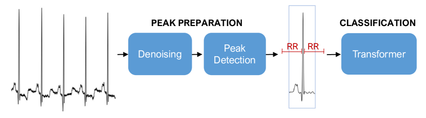
Figure 2: Overview of the ECG monitoring system.

III-A Peak preparation

The raw ECG signal goes through a denoising block performing baseline-wandering and noise removal. This block was structured according to the scheme suggested in [5], which includes two main filtering steps. The baseline wandering component is identified thanks to two median filters with respectively 200ms and 600ms window length, and subtracted from the signal. At this point, a low-pass filter with a cut-off frequency of 35Hz is exploited for powerline noise removal.

The clean signal is then processed for the identification of the window of interest around the R peak. Among the common QRS detection algorithms in the literature, here we refer to the well-known Pan-Tompkins detection algorithm, which allows the detection of 99.67% of the heartbeats in the considered dataset [21].

III-B Transformer for Arrhythmia recognition

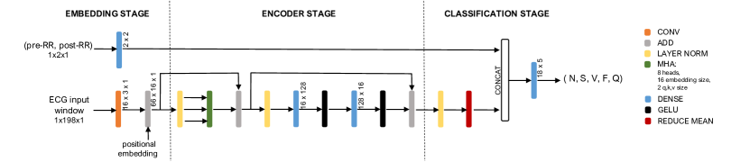
Figure 3: Architecture of the proposed transformer model for arrhythmia classification.

The proposed classifier is a Vision Transformer [22, 23], adapted for the processing of 1D medical signals, similarly to the approaches of [24, 25]. The model proposed in this work was developed starting from the architecture presented in [25], and further optimized for the arrhythmia recognition task. In alignment with the choice in [9], the input size is selected equal to 198 samples, equally distributed on the left and on the right of the considered R peak position within the heartbeat, and corresponding to roughly 0.5s of data based on the sampling frequency of the considered dataset.

The structure of the model is represented in Figure 3, and the values of the architectural parameters are reported in Table II. A typical ViT model consists of three main stages, an embedding stage, an encoder stage, and a classification stage. The embedding stage performs a data preparation task, producing as output a sequence of patches, inspired by the tokens of an input text, and including the positional information. In our model, this processing is obtained with a convolution stage, as proposed in [24]. The size k of the filtering kernels, applied considering no overlap with stride $s=k$, defines the length $S$ of the resulting sequence, whereas the size of each patch, the embedding size $E$, results from the selection of the number of output channels.

This sequence represents the input to the encoder stage, where most of the data processing is performed. The encoder is constituted by a stack of blocks including a Multi-Head-Attention (MHA) layer and a Feed Forward network, exploiting residual connections.

The MHA represents the most important mechanism within the transformer, allowing the evaluation of the mutual relevance between two points within the observed time series. As a first step for the attention evaluation, the input sequence of patches is projected into three different spaces, known as queries Q, keys K, and values V. The first two projections are used for the evaluation of the attention matrix, whose items allow to give weight to the elements within the third V projection, according to the Equation in 1, where $d$ represents the size of the Q, K, and V projections.

$$Attention(\textbf{{Q}},\textbf{{K}},\textbf{{V}})=Softmax(\frac{\textbf{{QK}}^{T}}{\sqrt{d}})\textbf{{V}}$$ (1)

The attention mechanism is usually replicated considering multiple parallel executions, called heads, where independent projections of the input are evaluated. In MHA, a final linear projection is performed in order to restore the embedding data size. In Table II, the number of heads is indicated with $H$.

The most relevant parameters impacting the computational load of the MHA layer were selected based on an exploration process aiming to maximize the accuracy on the target dataset, under a defined storage constraint. We considered as a first target a maximum of 512kB memory footprint, but we finally aimed at a more efficient topology that could fit the 128kB of the L1 memory of the targeted GAP9 processor. The exploration involved the selection of the embedding dimension $E$, the number of heads $H$, and the sequence length $S$ evaluated within the attention layer, deriving from the choice of the kernel size $k$ and stride $s$ within the embedding convolution layer. We also evaluated the dimension of the hidden layer of the encoder feed-forward network.

The final classification stage is usually implemented as an MLP or a Dense layer. Based on the results reported in the literature [10, 26, 4, 5], we considered the benefits of including the information about the RR intervals to differentiate the considered arrhythmia classes. We thus followed the example of [5] and introduced an additional input to the traditional transformer topology, representing the distance between the current R peak and the previous and following one. This second input is first linearly projected within the embedding stage and then concatenated to the output of the encoder which processes the ECG window around the heartbeat.

The tuple of values representing the RR intervals is normalized into the range [-2,2], to resemble the distribution of the encoder output at the concatenation level, thus simplifying the quantization process.

Stage	Layer	Output	Parameters
Embedding	Convolution	16$\times$66$\times$1	k: 3$\times$1
			s: 3
	Add Pos. Embedding	16$\times$66$\times$1
	Dense	1$\times$2
Encoder	Layer Norm	16$\times$66$\times$1
	Multi-Head-Attention	16$\times$66$\times$1	E: 16
			S: 66
			d: 2
			H: 8
	Layer Norm	16$\times$66$\times$1
	Dense	128$\times$66$\times$1
	Gelu	128$\times$66$\times$1
	Dense	16$\times$66$\times$1
	Gelu	16$\times$66$\times$1
Classification	Layer Norm	16$\times$66$\times$1
	Reduce Mean	1$\times$16
	Dense	1$\times$5

TABLE II: Parameters of the proposed transformer model for arrhythmia classification.

III-C Reference Datasets

As a main reference for this study, we considered the MIT-BIH Arrhythmia Database [11, 12], which collects the ECG recordings of 47 subjects into 48 records, lasting 30 minutes. The data included in the dataset is a composition of randomly selected ambulatory recordings from Boston’s Beth Israel Hospital, and recordings selected to include the clinically relevant arrhythmia examples. Each record reports the signal acquired by two channels, usually modified limb lead II (MLII) and V1, with a 360Hz sampling frequency. We refer in the following to processing based on the signal acquired by the MLII.

In alignment with most of the works in the literature [4, 5, 10, 26], we excluded from the training and test sets the records containing paced beats, namely ”102”, ”104”, ”107”, ”217”. Furthermore, we referred to the AAMI standard [27] to identify the 5 most relevant classification groups for the arrhythmia recognition problem: N (non-ectopic beats), S (supra-ventricular ectopic beats), V (ventricular ectopic beats), F (fusion beat), Q (unclassifiable beat).

Real-time heartbeat classification on wearable monitoring devices can be affected by different sources of noise. The MIT-BIH Noise Stress Test Database [28, 12] collects noise samples originating from three main sources, baseline wander, muscle artifacts, and electrode motion artifacts. In the following, we limit the analysis to the noise resulting from electrode motion artifacts, as it can modify significantly the appearance of the heartbeat and is not easily filtered out [28].

Here we describe the process leading to the creation of the noise-corrupted datasets referenced in the Experimental Section IV-C. The corruption of the signal is indicated as different Signal-to-Noise ratio (SNR) levels, expressed in dB. For brevity, we indicate as noiseless the original signal, with no additional noise deriving from electrode motion artifacts. Given a noiseless signal $S$ from the MIT-BIH Arrhythmia Database and a noise component $N$ from the MIT-BIH Noise Stress Test Database, the noise was scaled by a scaling factor $\alpha$ calculated based on the desired SNR, according to Equation 2.

$$\alpha=\sqrt{\frac{\text{mean}(|S|^{2})}{\text{mean}(|N|^{2})\times 10^{\frac{\text{desired SNR}}{10}}}}$$ (2)

The resulting noisy signal $Y$ is generated in Equation 3, where the scaling factor $\alpha$ results from Equation 2.

$$Y=S+\alpha\times N$$ (3)

Each noisy ECG signal is annotated with the original arrhythmia labels from the MIT-BIH Arrhythmia Database.

III-D Evaluation Metrics

As will be further detailed, Table III reports the typical composition of the training and test sets from the MIT-BIH dataset. As can be noticed, the dataset is highly unbalanced, presenting a majority of normal heartbeats and a different number of instances for each of the represented classes. Due to this reason, for the performance assessment, we not only considered the overall classification accuracy but also the sensitivity and precision on each of the targeted arrhythmia classes. The definition we referenced for these metrics is reported in equations 4 and 5, where we apply them to class N:

$$Sens_{N}=\frac{TN_{N}}{TN_{N}+FS_{N}+FV_{N}+FF_{N}+FQ_{N}}$$ (4)

$$Prec_{N}=\frac{TN_{N}}{TN_{N}+FN_{S}+FN_{V}+FN_{F}+FN_{Q}}$$ (5)

where the notation $TN_{N}$ indicates a normal sample, correctly classified as normal, $FS_{N}$ indicates a normal sample which is classified as a supra-ventricular ectopic beat, and finally $FN_{S}$ indicates a supra-ventricular ectopic beat classified as normal. A similar logic can be applied to the interpretation of the other symbols in the equations.

IV Experimental Results

In the following, we summarize the outcome of the tests performed to evaluate the performance of our proposed arrhythmia classifier.

IV-A Intra-patient arrhythmia recognition

We assessed the performance of our proposed model in the intra-patient classification task, based on 5-fold cross-validation. The ECG records in the dataset were segmented around each heartbeat corresponding to one of the NSVFQ arrhythmia classes, considering the dataset annotations for the heartbeat positioning. All collected segments were shuffled and randomly split into a training set, a validation set, and a test set, with a 7:1:2 ratio, to enable a direct comparison with the literature [5]. The composition of the dataset and a typical train-valid-test split is reported in Table III.

Arrhytmia Class	# Samples	Train	Valid	Test
N	90098	63022	9057	18019
S	2781	1967	273	541
V	7007	4919	664	1424
F	802	573	75	154
Q	15	12	1	2

TABLE III: Composition of the MIT-BIH dataset and typical training - validation - test split considered.

The training of the classifier was performed on one NVIDIA T4 Tensor Core GPU, using the TensorFlow framework inside the Google Colab environment. We exploited 200 epochs training, with Adam optimizer, adaptive reduce-on-plateau learning rate with starting value $2e-3$, and batch size 128.

The classification performance for full-precision inference is reported in Table V, in terms of mean value and standard deviation across the 5 tests considered. The performance of the model is only slightly impacted by the extremely low sensitivity and precision registered for the Q class, which is very under-represented in the dataset, and excluded from most studies [5, 4]. Our proposed model reaches an average of 99.05% accuracy on the 5 splits considered. Table V reports the summary confusion matrix referring to the cross-validation test. As can be derived from Table V, the main weakness is represented by a reduced sensitivity in the recognition of the F class.

Class	Sensitivity	Precision
N	99.74% (0.08)	99.38% (0.04)
S	88.79% (2.02)	94.14% (1.72)
V	96.91% (0.58)	97.59% (0.24)
F	76.92% (5.48)	88.99% (1.93)
Q	10% (20)	10% (20)
Accuracy tot	99.05% (0.08)

TABLE IV: Test classification performance, when no additional noise is applied to the signal. We report mean values and standard deviation in 5-fold cross-validation with full-precision inference.

True Labels	N	89867	119	79	31	2
	S	289	2468	23	1	0
	V	139	31	6783	45	0
	F	120	4	62	616	0
	Q	10	0	4	0	1
		N	S	V	F	Q
		Predicted Labels

TABLE V: Confusion matrix summarizing performance on the considered splits for the full-precision model, when no additional noise is applied to the signal.

IV-B Ablation Study

We report in the following the ablation study of the different data pre-processing choices explored, summarized in Table VI, limiting the analysis to a single train-test split.

The first line in the Table reports the accuracy of the selected model, depicted in Figure 3 of Section III-B. We started from the removal of the concatenation of the second input, representing the RR interval information, which helps in the arrhythmia class discrimination, as reported in several previous studies [10, 26, 4, 5]. The result was a 0.36% accuracy drop, reported in the second line.

We assessed at this point the relevance of the denoising step. We report in the third line the performance obtained when considering the RR information, but the selected topology was trained, validated, and tested on unfiltered data, not pre-processed with the denoising step in Figure 2. The resulting accuracy is lower than the best obtained by 0.51% points. To confirm this result, we finally removed both the RR concatenation and the denoising step, thus obtaining the performance reported in the fourth line. As can be observed, there is no further accuracy degradation compared to the number reported in the third line, showing how the RR information only provides a relevant advantage when combined with an effective denoising approach.

Model	Test Accuracy
Selected Model	99.17%
no RR	98.81%
no denoising	98.66%
no RR and no denoising	98.69%

TABLE VI: Comparison of test performance on a single 7:1:2 split, based on different input processing choices. Accuracy numbers refer to tests performed with no additional noise applied to the signal.

IV-C Post-deployment evaluation

This work targets wearable devices for real-time heartbeat classification, we thus present in this section the assessment of the performance degradation deriving from two main challenges of wearable deployment, namely increasing levels of noise corrupting the ECG signal and accuracy loss due to data quantization.

IV-C1 Noise degradation

As a first step for the noise degradation analysis, we used as a baseline the accuracy reported in Table VI, deriving from the evaluation on the noiseless signal, and the corresponding specific train-test split. We repeated the same test using noise-augmented versions of the dataset samples in training and in test, to create Figure 4. Different lines correspond to different levels of noise used for augmenting the training set, while different evaluation points in each line correspond to a different level of noise in the test. Considered levels are noiseless, 24dB SNR, 10dB SNR, 3dB SNR, and balanced mix, where noiseless corresponds to the original non-augmented dataset samples and balanced mix corresponds to an equally partitioned test set, with different noise levels applied to each subset, to emulate real-life conditions where the noise level is expected to vary over an evaluation.

The solid grey line shows the results obtained when performing classification on different test conditions with the model trained on the non-corrupted signal. As can be observed, in this case, the accuracy is dramatically affected by the noise, with up to almost 8% points drop registered with high noise levels and test SNR equal to 3dB.

In order to improve robustness during real-time inference, we considered the effect of including examples of corrupted signals during the training process, represented by the other lines in the plot. As can be observed, augmenting with a specific level of noise improves the resilience of the classification algorithm when a similar noise level is considered in the test, although in general, it determines a slight degradation for lower noise levels. The balanced mix strategy, on the other hand, performs better than specific levels in most evaluation points and especially in the leftmost one, representing real-life conditions. It reduces the accuracy drop on the most corrupted signal (SNR = 3dB) to less than 1.2% points. This gain in the robustness to high noise levels does not compromise the classification accuracy on the noiseless signal, which is only 0.02% lower than the highest one reported in Table VI. The results thus confirmed the advantages of a training approach considering a variable noise level for augmentation.

Based on these findings, we repeated 5-fold cross-validation using training data augmentation and reported the results in Table IX. The first two columns summarize the performance for the classification of the noiseless signal. The average accuracy is 99.07%, thus no degradation is observed compared to the un-augmented training approach. The confusion matrix is also included for completeness and reported in Table IX.

	Noiseless Test		Balanced Mix Test
Class	Sensitivity	Precision	Sensitivity	Precision
N	99.73% (0.08)	99.42% (0.08)	99.59% (0.12)	99.15% (0.08)
S	89.13% (1.1)	93.64% (1.34)	84.08% (1.2)	91.34% (1.62)
V	97% (0.42)	98.01% (0.33)	95.7% (0.42)	96.59% (0.47)
F	78.73% (4.97)	88.63% (3.42)	71.05% (4.34)	84.62% (5.15)
Q	4% (8)	10% (20)	2% (4)	2.5% (5)
Accuracy	99.07% (0.06)		98.65% (0.07)

TABLE VII: Test classification performance, reporting mean values and standard deviation in 5-fold cross-validation with full-precision inference, when training data augmentation with varying noise levels is exploited.

True Labels	N	89858	136	50	37	17
	S	278	2479	22	2	0
	V	130	33	6789	44	2
	F	104	1	64	631	2
	Q	11	0	3	0	1
		N	S	V	F	Q
		Predicted Labels

TABLE VIII: Confusion matrix summarizing noiseless test performance on the considered splits for the full-precision model, when training data augmentation with varying noise levels is exploited.

True Labels	N	358901	710	483	232	66
	S	1630	9355	130	8	1
	V	807	182	26802	192	9
	F	596	4	325	2278	5
	Q	47	0	11	0	2
		N	S	V	F	Q
		Predicted Labels

TABLE IX: Confusion matrix summarizing balanced mix test performance on the considered splits for the full-precision model, when training data augmentation with varying noise levels is exploited.

On the other hand, a significant advantage was obtained on the balanced mix test. In this scenario, 98.65% was achieved on average on the 5 train-test splits considered. The corresponding cumulative confusion matrix is reported in Table IX. As can be observed, each test sample was replicated in order to represent a different noise condition in real-time inference. The resulting evaluation metrics are summarized in the right columns of Table IX. The comparison with the performance on the noiseless test shows a generally reduced sensitivity and precision, especially in the recognition of the S and F classes.

Figure 4: Test classification performance considering increasing levels of noise deriving from electrode motion artifacts.

IV-C2 Quantization

Finally, in order to optimize the storage requirements of our model and exploit at best the byte processing resources on edge-processing platforms, we made use of the Quantlab framework [29] to obtain 8-bit quantization. To this aim, we considered the models trained with noise augmentation and whose full-precision performance is summarized in Table IX. We exploited 15 epochs of quantization-aware fine-tuning, obtaining an average test accuracy of 98.97% on the clean noiseless signal, with a limited 0.1% drop from the accuracy of the full-precision models. The performance metrics are summarized in the first two columns of Table XII, whereas the confusion matrix is reported in Table XII. The accuracy drop resulted from restricting all computations to integer type, and it mostly affects the sensitivity of the S class, as can be observed from the table.

We finally tested the performance on the classification of noise-corrupted signal, with the balanced mix test. The outcome is reported in the third and fourth columns of Table XII, and a summary confusion matrix is reported in Table XII. The assessment resulted in an average 98.36% accuracy, which we can consider as a worst-case post-deployment real-time performance prediction.

	Noiseless Test		Balanced Mix Test
Class	Sensitivity	Precision	Sensitivity	Precision
N	99.74% (0.05)	99.3% (0.08)	99.41% (0.14)	99.01% (0.1)
S	84.73% (1.1)	94.65% (0.87)	78.3% (1.55)	92.12% (0.8)
V	97.52% (0.42)	97.24% (0.45)	96.34% (0.53)	94.11% (1.26)
F	76.58% (3.52)	89.56% (2.57)	68.94% (2.62)	81.33% (4.45)
Q	9% (11.14)	40% (48.99)	5.75% (7.57)	4.48% (6.84)
Accuracy	98.97% (0.04)		98.36% (0.08)

TABLE X: Test classification performance, reporting mean values and standard deviation in 5-fold cross-validation with 8-bit inference, when training data augmentation with varying noise levels is exploited.

True Labels	N	89860	115	88	32	3
	S	388	2356	37	0	0
	V	115	17	6825	40	1
	F	121	1	66	614	0
	Q	10	0	3	0	2
		N	S	V	F	Q
		Predicted Labels

TABLE XI: Confusion matrix summarizing noiseless test performance on the considered splits for the 8-bit model, when training data augmentation with varying noise levels is exploited.

True Labels	N	358267	647	1061	344	73
	S	2126	8708	282	7	1
	V	743	93	26971	169	16
	F	645	3	345	2211	4
	Q	46	0	9	0	5
		N	S	V	F	Q
		Predicted Labels

TABLE XII: Confusion matrix summarizing balanced mix test performance on the considered splits for the 8-bit model, when training data augmentation with varying noise levels is exploited.

IV-D Comparison with the state of the art

We discuss at this point how our proposed solution compares to the state-of-the-art context, considering as a main reference the work of [5], which represents the most accurate alternative. Table XIII summarizes the most relevant performance figures for the comparison. The first line refers to full-precision inference performed on noiseless data, as we indicate the data not corrupted with electrode motion noise. A limited accuracy drop is observed when evaluating the performance of the 8-bit model, in the second line. Our result presents only a slight degradation with respect to the performance of the state-of-the-art transformer model, corresponding to only a 0.65% accuracy drop, despite the reduced complexity in terms of the number of parameters and memory footprint, reported in the fifth and sixth lines.

Finally, although a direct comparison with the reference model is not possible, we provide an assessment of worst-case performance considering a deployment scenario corrupted by different levels of noise. The training data augmentation allowed us to limit the accuracy drop to 0.4% points for full-precision inference, whereas post-deployment assessment of the quantized model results in 98.36% average accuracy, which we report in Table I as the worst-case expected real-time deployment performance.

Metric	This Work	[5]
32-bit Accuracy Noiseless	99.05%	99.62%
8-bit Accuracy Noiseless	98.97%	-
32-bit Accuracy Noisy	98.65%	-
8-bit Accuracy Noisy	98.36%	-
Parameters	6649	405711 1
Footprint	49kB	3MB1

• Estimated from the paper.

TABLE XIII: Comparison with the state-of-the-art transformer model for arrhythmia recognition.

V Deployment

In this section, we assess the efficiency of the proposed transformer classifier, considering its deployment on the parallel ultra-low power (PULP) GAP9 processor [19]. This commercial platform embeds a computing cluster of 8 parallel processors, accessing a shared 128kB L1 memory to enable efficient parallel execution. The offload of computations to the cluster is handled by an additional core, working as a Fabric Controller. The memory system includes also a 1.5MB L2 memory and supports voltage and frequency tuning for power management. Based on the recent assessment on the tiny-ML benchmarks [30], GAP9 shows exceptional energy efficiency, with as low as 0.33mW/GOP, thus representing a perfect fit for long-term wearable monitoring tasks. Furthermore, the computational workload of the transformer model is intrinsically parallel, thus the computing cluster can be efficiently exploited to reduce inference time during real-time execution.

For efficient deployment, we considered the 8-bit model reported in Table XIII. We exploited the Dory code generation tool [31] for assisted implementation on the target platform. As depicted in Figure 5, over 67% of the computing time is occupied by the MHA layer, whose implementation exploits the parallel resources on the platform by balancing the computation among the cores of the computing cluster: each head is mapped into one of the eight cores, according to the strategy described in [32]. Measured on-hardware performance results in as low as 4.28ms/inference and 0.09mJ energy consumption, for parallel execution exploiting 8 cores at 240MHz working frequency. As can be noticed from the measurements reported in Table XIV, this operating configuration was selected as the most energy-efficient one. The power measurements were performed with a Power Profiler Kit II (PPK2) connected to the GAP9 Evaluation Kit, resulting in an average power consumption of 20.33mW.

Figure 5: Composition of the computational workload of the different operators in the proposed model, expressed as percentage of the total inference time.

	GAP9
Frequency	370 MHz	240 MHz
Time/Inf	2.85 ms	4.28 ms
Power	42.60 mW	20.33 mW
Energy/Inf	0.12 mJ	0.09 mJ

TABLE XIV: On-hardware performance on the GAP9 processor for parallel execution on the 8 cores of the computing cluster.

VI Conclusions

In this work, we presented an efficient transformer model for arrhythmia classification, reaching 99.05% accuracy in the classification of the 5 most common arrhythmia classes from the MIT-BIH Arrhythmia database. The classification performance was assessed considering different inference conditions, resembling real-time disturbance, by introducing different levels of noise corruption deriving from electrode motion artifacts, based on the noise samples from the MIT-BIH Noise Stress Test database.

Integer 8-bit inference resulted in 98.97% accuracy on the noiseless signal, which is only 0.65% lower than the state-of-the-art transformer model, although reducing by 60$\times$ the number of parameters, and by 300$\times$ the number of operations. The lean topology of the proposed model can be efficiently deployed on low-power devices for wearable monitoring, as it is demonstrated by the performance evaluated on the GAP9 parallel processor, where inference is executed in 4.28ms, with 0.09mJ energy consumption.

References

- [1] W. H. Organization, “Cardiovascular diseases,” June 2023. [Online]. Available: https://www.who.int/health-topics/cardiovascular-diseases#tab=tab_1
- [2] S. M. A. Iqbal, I. Mahgoub, E. Du, M. A. Leavitt, and W. Asghar, “Advances in healthcare wearable devices,” npj Flexible Electronics, vol. 5, no. 9, 2021. [Online]. Available: https://doi.org/10.1038/s41528-021-00107-x
- [3] C.-F. Zhao, W.-Y. Yao, M.-J. Yi, C. Wan, and Y.-l. Tian, “Arrhythmia classification algorithm based on a two-dimensional image and modified efficientnet,” Computational Intelligence Neuroscience, 2022.
- [4] R. Hu, J. Chen, and L. Zhou, “A transformer-based deep neural network for arrhythmia detection using continuous ecg signals,” Computers in Biology and Medicine, vol. 144, p. 105325, 2022. [Online]. Available: https://www.sciencedirect.com/science/article/pii/S0010482522001172
- [5] G. Yan, S. Liang, Y. Zhang, and F. Liu, “Fusing transformer model with temporal features for ecg heartbeat classification,” in 2019 IEEE International Conference on Bioinformatics and Biomedicine (BIBM), 2019, pp. 898–905.
- [6] P. K. Singh, N. Shukla, A. Pandey, A. P. Shukla, and S. C. Neupane, “Ecg-vit: A transformer-based ecg classifier for energy-constraint wearable devices,” Journal of Sensors, p. 2449956, 2022. [Online]. Available: https://doi.org/10.1155/2022/2449956
- [7] W. Wang, J. Guan, X. Che, and W. Wang, “Ms-mlp: Multi-scale sampling mlp for ecg classification,” in 2022 30th European Signal Processing Conference (EUSIPCO), 2022, pp. 1288–1292.
- [8] A. A. Ahmed, W. Ali, T. A. A. Abdullah, and S. J. Malebary, “Classifying cardiac arrhythmia from ecg signal using 1d cnn deep learning model,” Mathematics, vol. 11, no. 3, 2023. [Online]. Available: https://www.mdpi.com/2227-7390/11/3/562
- [9] M. A. Scrugli, D. Loi, L. Raffo, and P. Meloni, “An adaptive cognitive sensor node for ecg monitoring in the internet of medical things,” IEEE Access, vol. 10, pp. 1688–1705, 2022.
- [10] M. M. Farag, “A tiny matched filter-based cnn for inter-patient ecg classification and arrhythmia detection at the edge,” Sensors, vol. 23, no. 3, 2023. [Online]. Available: https://www.mdpi.com/1424-8220/23/3/1365
- [11] G. Moody and R. Mark, “The impact of the mit-bih arrhythmia database,” IEEE Engineering in Medicine and Biology Magazine, vol. 20, no. 3, pp. 45–50, 2001.
- [12] A. Goldberger, L. Amaral, L. Glass, J. Hausdorff, P. C. Ivanov, R. Mark et al., “Physiobank, physiotoolkit, and physionet: Components of a new research resource for complex physiologic signals.” Circulation, vol. 101, p. e215–e220, 2000.
- [13] D. L. T. Wong, Y. Li, D. John, W. K. Ho, and C.-H. Heng, “Low complexity binarized 2d-cnn classifier for wearable edge ai devices,” IEEE Transactions on Biomedical Circuits and Systems, vol. 16, no. 5, pp. 822–831, 2022.
- [14] G. Sivapalan, K. K. Nundy, S. Dev, B. Cardiff, and D. John, “Annet: A lightweight neural network for ecg anomaly detection in iot edge sensors,” IEEE Transactions on Biomedical Circuits and Systems, vol. 16, no. 1, pp. 24–35, 2022.
- [15] J. Liu, J. Fan, Z. Zhong, H. Qiu, J. Xiao, Y. Zhou, Z. Zhu, G. Dai, N. Wang, Q. Liu, Y. Xie, H. Liu, L. Chang, and J. Zhou, “An ultra-low power reconfigurable biomedical ai processor with adaptive learning for versatile wearable intelligent health monitoring,” IEEE Transactions on Biomedical Circuits and Systems, vol. 17, no. 5, pp. 952–967, 2023.
- [16] C. Che, P. Zhang, M. Zhu, Y. Qu, and B. Jin, “Constrained transformer network for ecg signal processing and arrhythmia classification,” BMC Medical Informatics and Decision Making, p. 184, 2021. [Online]. Available: https://doi.org/10.1186/s12911-021-01546-2
- [17] A. Natarajan, Y. Chang, S. Mariani, A. Rahman, G. Boverman, S. Vij, and J. Rubin, “A wide and deep transformer neural network for 12-lead ecg classification,” in 2020 Computing in Cardiology, 2020, pp. 1–4.
- [18] L. Meng, W. Tan, J. Ma, R. Wang, X. Yin, and Y. Zhang, “Enhancing dynamic ecg heartbeat classification with lightweight transformer model,” Artificial Intelligence in Medicine, vol. 124, p. 102236, 2022. [Online]. Available: https://www.sciencedirect.com/science/article/pii/S093336572200001X
- [19] Greenwaves, “Ultra low power gap processors,” August 2023. [Online]. Available: https://greenwaves-technologies.com/low-power-processor/
- [20] V. Kartsch, G. Tagliavini, M. Guermandi, S. Benatti, D. Rossi, and L. Benini, “Biowolf: A sub-10-mw 8-channel advanced brain–computer interface platform with a nine-core processor and ble connectivity,” IEEE Transactions on Biomedical Circuits and Systems, vol. 13, no. 5, pp. 893–906, 2019.
- [21] J. Pan and W. J. Tompkins, “A real-time qrs detection algorithm,” IEEE Transactions on Biomedical Engineering, vol. BME-32, no. 3, pp. 230–236, 1985.
- [22] D. Alexey, B. Lucas, K. Alexander, W. Dirk, Z. Xiaohua, U. Thomas, D. Mostafa, M. Matthias, H. Georg, G. Sylvain, U. Jakob, and H. Neil, “An image is worth 16x16 words: Transformers for image recognition at scale,” International Conference on Learning Representations, 2021.
- [23] A. Vaswani et al., “Attention is all you need,” Advances in Neural Information Processing Systems, vol. 2017-December, p. 5999 – 6009, 2017.
- [24] A. Burrello, F. B. Morghet, M. Scherer, S. Benatti, L. Benini, E. Macii, M. Poncino, and D. J. Pagliari, “Bioformers: Embedding transformers for ultra-low power semg-based gesture recognition,” IEEE 2022 DATE, 2022.
- [25] P. Busia, A. Cossettini, T. M. Ingolfsson, S. Benatti, A. Burrello, M. Scherer, M. A. Scrugli, P. Meloni, and L. Benini, “Eegformer: Transformer-based epilepsy detection on raw eeg traces for low-channel-count wearable continuous monitoring devices,” in 2022 IEEE Biomedical Circuits and Systems Conference (BioCAS), 2022, pp. 640–644.
- [26] T. Wang, C. Lu, Y. Sun, M. Yang, C. Liu, and C. Ou, “Automatic ecg classification using continuous wavelet transform and convolutional neural network,” Entropy, vol. 23, no. 1, 2021. [Online]. Available: https://www.mdpi.com/1099-4300/23/1/119
- [27] A. for the Advancement of Medical Instrumentation American National Standards Institute, Testing and Reporting Performance Results of Cardiac Rhythm and ST-segment Measurement Algorithms, ser. ANSI/AAMI. The Association, 1999. [Online]. Available: https://books.google.it/books?id=gzPdtgAACAAJ
- [28] M. R. Moody G.B., Muldrow W.E., “A noise stress test for arrhythmia detectors.” Computers in Cardiology, vol. 11, pp. 381–384, 1984.
- [29] M. Spallanzani, G. Rutishauser, M. Scherer, A. Burrello, F. Conti, and L. Benini, “QuantLab: a Modular Framework for Training and Deploying Mixed-Precision NNs,” https://cms.tinyml.org/wp-content/uploads/talks2022/Spallanzani-Matteo-Hardware.pdf, March 2022.
- [30] ML Commons, “Inference: tiny. v1.0 Results,” 2023, Accessed: 01-08-2023. [Online]. Available: https://mlcommons.org/en/inference-tiny-10/
- [31] A. Burrello, A. Garofalo, N. Bruschi, G. Tagliavini, D. Rossi, and F. Conti, “Dory: Automatic end-to-end deployment of real-world dnns on low-cost iot mcus,” IEEE Transactions on Computers, pp. 1–1, 2021.
- [32] A. Burrello, M. Scherer, M. Zanghieri, F. Conti, and L. Benini, “A microcontroller is all you need: Enabling transformer execution on low-power iot endnodes,” 2021 IEEE International Conference on Omni-Layer Intelligent Systems (COINS), pp. 1–6, 2021.