The simulation of distributed quantum algorithms

Abstract

We study distributed quantum computing (DQC), the use of multiple quantum processing units to simulate quantum circuits and solve quantum algorithms. The nodes of a distributed quantum computer consist of both local qubits, essential for local circuit operations, and communication qubits, extending circuit capabilities across nodes. We created a distributed quantum circuit simulator (DQCS) written in Qiskit, which we use to simulate a quantum circuit on multiple nodes, show its applicability for distributed quantum phase estimation, amplitude estimation. We use DQCS to study the scaling of DQC for the quantum state preparation of a probability (normal) distribution.

1 Introduction

To make quantum computing advantageous in industry, the scalability of available quantum computing hardware needs to be greatly increased. Distributed quantum computing (DQC) [1, 2] provides a way to scale by using several quantum processing units (QPUs) are connected through communication links (optical fibers or superconducting wires) [3, 4] to increase the available computational resources. The schema for DQC is shown in Fig. 1, where the nodes consist of local processing units and communication units. The local processing units consist of local qubits, and the communication unit consists of communication qubits that could be entangled between the nodes [5, 6].

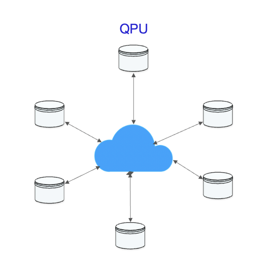
Figure 1: Distributed quantum computer with multiple quantum processing units (QPU)

In this paper, we describe a distributed quantum computing simulator (DQCS) that uses non-local quantum gates between the nodes, creates distributed quantum circuits, and evaluates their performance in the presence of noise [7]. We use the DQCS to study distributed quantum algorithms [8, 9, 10], show the applicability of the dynamic quantum circuits in DQC that reduce the resource overhead, and help achieve high fidelity with the example of distributed quantum phase estimation (DQPE). We study the probability distribution loading in DQC, scaling with the number of nodes. We use the DQCS to run the distributed quantum amplitude estimation (DQAE) algorithm on multiple nodes. The DQCS contains modules that provide users various ways to study, run, and evaluate the performance of quantum algorithms in distributed quantum computer [9]. When we increase the number of qubits in the same device, the noise from the cross-talk reduces the fidelity of the quantum algorithm. DQC provides a approach where we could use multiple QPUs with fewer qubits to run quantum algorithms. The DQCS provides a platform to study their performance.

2 Distributed quantum computing simulator

The DQCS is a comprehensive package that consists of the following modules:

• Non-local quantum gates: This module facilitates the application of non-local quantum gates [7] between qubits residing in different nodes. It enables quantum gates to span across nodes, allowing for the execution of more complex distributed quantum algorithms.

• Distributed circuits: The distributed circuits module enables users to effortlessly create distributed quantum circuits using a node dictionary and a quantum circuit. It automatically handles communication registers, preventing users from explicitly specifying them.

• Create distributed circuits: For advanced users seeking more control, this module offers flexibility where the user can provide input to the communication register, allowing us to simulate complicated quantum circuits.

• Noise model: To enhance the fidelity of simulations, the library offers optional noise model module. This component incorporates realistic noise modeling, including single-qubit and two-qubit errors, providing a more accurate representation of real-world quantum systems.

The steps to run the simulator are as follows:

1. Create a quantum circuit using Qiskit. Instantiate the distributed circuits with your quantum circuit and the nodes to obtain the distributed quantum circuit.

   ⬇

   from qiskit import QuantumCircuit

   import distributed

   qc = QuantumCircuit(3)

   qc.h(0)

   qc.h(1)

   qc.cx(0, 2)

   nodes = {"1": [0, 1], "2": [2]}

   gate_app, circuit = distributed.DistributedCircuits(qc, nodes). create_circuit()

   The circuit gives the distributed quantum circuit the parameter $gate\textunderscore app=1$ for the successful creation of the distributed quantum circuit.

2. Alternatively, use the $CreateDistributedCircuits$ instance with the quantum circuit, communication qubits, nodes, and the probability $p$ (coupling efficiency for the node) to create the distributed quantum circuit. Let us consider the example to illustrate the module.

   ⬇

   from qiskit import QuantumCircuit

   from qiskit import QuantumRegister, ClassicalRegister

   import distributed

   q_0 = QuantumRegister(2, ’a’)

   q_1 = QuantumRegister(2, ’b’)

   qc = QuantumCircuit(q_0, q_1)

   nodes = {"1": [q_0[0], q_0[1]], "2": [q_1[0]], "3": [q_1[1]]}

   qc.h(q_0[0])

   qc.cx(q_0[1], q_1[1])

   #Define an empty circuit with communication registers

   comm = QuantumRegister(4, ’c’)

   c = ClassicalRegister(4, ’cl’)

   circ = QuantumCircuit(q_0, q_1, comm, c)

   gate_app, circuit = distributed.CreateDistributedCircuits(qc, c, circ, comm, nodes, 1). create_circuit()

   The probability p=1 in the above example is the qubit-node coupling efficiency.

3. Instantiate the noise model with your distributed quantum circuit, specifying parameters such as the number of shots, repetitions, and error probabilities (single, two-qubit gate, measurement, reset errors).

2.1 Noise model

The noise in the quantum computation can be simulated using Qiskit’s noise model [11]. Here, we give a brief description of the noise model. The depolarization channel $E$ acts on the quantum state of $n$ qubits $\rho$, $\rho\rightarrow E(\rho)$,

$$E(\rho)=(1-\lambda)\rho+\lambda Tr(\rho)\otimes\frac{I_{2^{n}}}{2^{n}},$$ (1)

where $\lambda$ is the depolarization rate, $Tr(\rho)$ is the partial trace of $n$ qubits, and $I_{2^{n}}$ is the identity $2^{n}\times 2^{n}$ matrix, respectively. The single qubit gate error channel $E$ could be obtained using the depolarization channel for $n=1$. Here, $\rho$ is the quantum state before the application of the single qubit quantum gate ($U$) on the $i$th qubit. The channel gives $U_{i}\rho U_{i}^{\dagger}\rightarrow\rho^{\prime}$,

$$\rho^{\prime}=(1-\epsilon_{d})U_{i}\rho U_{i}^{\dagger}+\epsilon_{d}Tr_{i}(\rho)\otimes\frac{I_{2}}{2},$$ (2)

where $\epsilon_{d}$ is the single qubit gate error rate and $Tr_{i}$ is the partial trace of the $i^{th}$ qubit. Let us consider a two-qubit quantum gate $U_{i,j}$ (between the qubits $i$ and $j$). The two-qubit gate error channel could be obtained for $n=2$ that applies the transformation $U_{ij}\rho U_{ij}^{\dagger}\rightarrow\rho^{\prime\prime}$.

$$\rho^{\prime\prime}=(1-\epsilon_{g})U_{ij}\rho U_{ij}^{\dagger}+\epsilon_{g}Tr_{i,j}(\rho)\otimes\frac{I_{4}}{4}$$ (3)

where $\epsilon_{g}$ is the two-qubit gate error rate and $Tr_{i,j}$ is the partial trace of the qubits $(i,j)$. The fidelity of the quantum circuit after one successful implementation of the non-local CNOT gate (up to the first order) is $\epsilon\approx(\epsilon_{d}+\epsilon_{g})$. If we consider $\epsilon_{m}$, to denote the measurement reset error, we may approximate the fidelity for $N$ distributed quantum gates, $F\approx{(1-(\epsilon_{d}+\epsilon_{g}+2\epsilon_{m}))}^{N}$.

3 Distributed quantum algorithms

Quantum algorithms are utilized to achieve speedup for various applications, including machine learning, optimization [12], credit risk analysis [13], and option pricing using Monte Carlo integration [14, 15, 16]. We consider the simulation of two distributed quantum algorithms, DQPE and DQAE, respectively.

3.1 Distributed dynamic quantum phase estimation

In the distributed quantum circuit, there is opportunity to replace non-local quantum gates with dynamic quantum circuits, which is advantageous for quantum algorithms. We demonstrate the dynamic quantum Fourier transform without two-qubit quantum gates. Let’s consider a quantum circuit for the QFT on three qubits in Fig. 2.

@C=1.0em @R=0.2em @!R q_0 & H 1       P(-π/2) 2
q_1 H       P(-π/4) 1       P(-π/2)
q_2 H

Figure 2: Quantum Fourier transform on three qubits

The corresponding dynamic quantum circuit is shown in the Fig. 3.

@C=2.0em @R=1em @!R q_0 & H
q_1 P(-π/2) [-1] H
q_2 P(-π/4) [-1] P(-π/2) [-1] H

Figure 3: Dynamic quantum Fourier transform on three qubits

We can now illustrate the application of distributed dynamic QFT in quantum phase estimation (QPE). This problem involves determining the eigenvalue of the unitary gate that acts as $U|\psi\rangle=e^{2i\pi y}|\psi\rangle$, where $|\psi\rangle$ is the eigen-state of $U$, and $y$ is a fraction corresponding to the eigenvalue. The quantum circuit used to implement QPE is shown in Fig. 4.

@C=1.5em @R=0.8em @!R —0⟩ & H 3 H
—0⟩ H 2 P(-π/2) [-1] H
—0⟩ H 1 P(-π/4) [-1] P(-π/2) [-1] H
—ψ⟩ U^2^2 U^2^1 U^2^0

Figure 4: Distributed dynamic quantum phase estimation

We can obtain the fraction $y$ using the measurement outcome. Suppose we obtain the measurement outcome $y_{0}y_{1}y_{2}$, where $y_{i}\in\{0,1\}$, then the fraction $y$ is given by $(y_{0}y_{1}y_{2})_{10}/2^{3}$. Let us consider the example of the implementation of QPE for the unitary $U=R_{X}(\pi)\otimes R_{Y}(\pi)$ gate acting on two qubits; one of the eigenvalues for the operators is $-1$ ($y=1/2$, which corresponds to the measurement output = $100$). We prepare the eigen-state $|\psi\rangle$, create the distributed QPE (DQPE) for the following qubit distributions: 1: [0, 1, 2], 2: [3, 4], and apply the dynamic QFT to the distributed quantum circuit. The probability of the outcome is shown in Fig. 5.

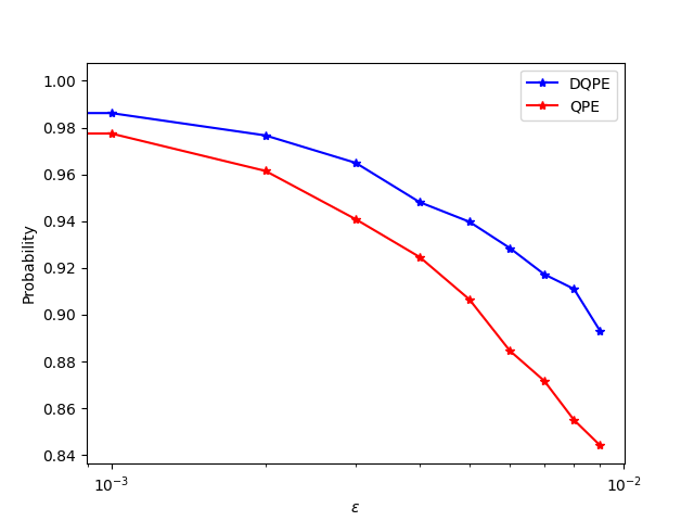
Figure 5: The probability of the outcome for the distributed QPE (DQPE) (blue) vs. QPE (red) in the presence of noise $\epsilon_{d}=\epsilon_{g}=\epsilon$, $\epsilon_{m}=0$

3.2 Distributed quantum amplitude estimation

Quantum amplitude estimation (QAE) is used to calculate the unknown amplitude of a quantum state, which has applications such as the calculation of the expectation value of the discrete linear function, quantum Monte Carlo integration [14, 16], quantum risk analysis, and portfolio optimization. Here, we use the DQCS to simulate distributed QAE (DQAE) using multiple nodes. There are multiple approaches to performing QAE. We study the problem of DQAE using the maximum likelihood estimation [17] that does not use the QFT to achieve quadratic speedup over classical Monte Carlo algorithms in DQC. We show that the estimation error for the DQAE [17], simulated using the DQCS, achieves the Cramer-Rao bound, which provides a way to scale QAE using multiple QPUs. We provide a brief introduction to QAE, the unitary operator $A$.

$$A|0\rangle_{n+1}=\sqrt{1-a}|\psi_{0}\rangle_{n}|0\rangle+\sqrt{a}|\psi_{1}\rangle_{n}|1\rangle,$$ (4)

where $a$ is the unknown amplitude to be estimated, and $|\psi_{0}\rangle_{n}$ and $|\psi_{1}\rangle_{n}$ are (normalized) good and bad states, respectively, that correspond to the probability of measurement of $0\rangle$ and $|1\rangle$ in the last qubit, respectively. We could prepare the $A$ operator, using the probability distribution loading $P(x)$ [14], that loads a discrete probability distribution to a quantum state, the bounded function $f(x)$ constructed from the samples of $P(x)$ realized using multiple controlled-$R_{y}$ gates with controlled-$R_{y}(f(i))$ on gate on the $ith$ qubit [14]. The probability of the measurement of $|1\rangle$ on the last qubit gives the expectation value $\mathrm{E}[f(x)]$.

$$\mathrm{E}[f(x)]=\sum_{i=0}^{2^{n}-1}p(x_{i})f(x_{i}),$$ (5)

Suppose P(x) is a uniform distribution, the probability of measuring $|1\rangle$ on the last qubit is given by $\frac{1}{2^{n}}\sum_{i=0}^{2^{n}-1}f(x_{i})$ for $x_{i}=i/2^{n}$ [15]. For QAE, we construct the $Q$ operator such that $Q=-AS_{0}A^{-1}S_{X}$. The operator $S_{X}$ leaves the good states unchanged and includes a phase $(-1)$ on the bad states. $S_{X}|\psi_{0}\rangle|0\rangle=|\psi_{0}\rangle|0\rangle$, $S_{X}|\psi_{1}\rangle|1\rangle=-|\psi_{1}\rangle|1\rangle$, the operator $S_{0}$ attaches a phase (-1) to $|0\rangle_{n}$, leave other basis states unchanged, the repeated application of $Q$, $m$ times on the state $A|0\rangle$ give

$$Q^{m}|\psi\rangle=\cos(2m+1)\theta|\psi_{0}\rangle|0\rangle+\sin(2m+1)\theta|\psi_{1}\rangle|1\rangle,$$ (6)

QAE requires multiple controlled-unitary gates for the implementation of the reflection operators. We could write multiple CNOT gates (with $n$ control qubits and a single-qubit unitary) with single-qubit gates and $\leq(20n-38)$ CNOT gates [18, 7]. We consider the QAE without phase estimation that uses the maximum likelihood estimate [17] for the integration of $\int_{0}^{c}\sin^{2}(x)$ in DQC. We compare the estimated error values against the Cramer-Rao bound [17], where $P(x)$ is a uniform distribution obtained by applying Hadamard gates to all the qubits. The function $f(x)$ is prepared with $a=c/2^{n-1},b=c/2^{n}$ using 1 $R_{y}$ gate and $n$ controlled-Ry gates, $Ry(c/2^{n-i})$ [17]. It could be seen in Fig. 6 (($c=\frac{\pi}{3}$)) that DQAE could be simulated, and the estimated value achieves the Cramer-Rao bound.

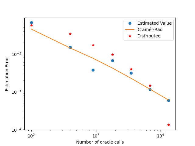
Figure 6: The estimated value in quantum computer (1 node), distributed quantum computer (2 nodes), Cramer-Rao bound [17]

3.3 Probability distribution loading in DQC

We will now consider the quantum state preparation of a normal distribution in DQC. The normal distribution

$$P(X=x)=\frac{1}{\sqrt{2\pi\sigma^{2}}}e^{\frac{-(x-\mu)^{2}}{\sigma^{2}}},$$ (7)

loaded to quantum state $|p\rangle=\sum_{i=0}^{2^{d-1}}\sqrt{p_{i}}|x_{i}\rangle$, where $p_{i}$ is sampled from $P(x)$ with $2^{d}$ points [14, 15]. We use DQCS to simulate the quantum state preparation of a probability distribution. We consider the normal distribution with $8$ qubits with the mean $\mu=1$ and $\sigma=2$ in DQCS, with $n=1,2,4,8$ nodes, to obtain the Heilinger fidelity in Fig. 7.

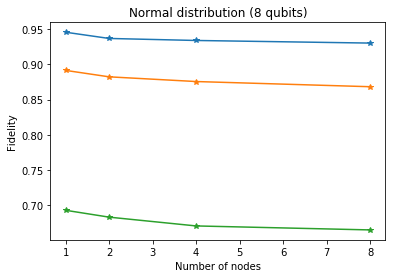
Figure 7: The Heilinger fidelity of a normal distribution with 8 qubits with different numbers of nodes, where $\epsilon=(0.002,0.005,0.009)$

4 Conclusion

We described a distributed quantum circuit simulator [19, 20, 21, 22] written in the Qiskit, utilizing multiple interconnected quantum processing units (QPUs) with local and communication qubits. We simulated distributed quantum algorithms, analyzed their performance under noise, and showed the applicability of dynamic quantum circuits in DQC. We considered quantum Monte Carlo integration, which is applicable to other problems such as portfolio optimization and credit risk analysis using the DQCS. We studied the scaling of the probability distribution loading in DQC in the presence of imperfection. It is also possible to use DQCS to study quantum algorithms in quantum networks [23] [24]. In the future, we could study distributed quantum machine learning algorithms for classification and regression [25].

References

- [1] M.. al. “Towards Distributed Quantum Computing by Qubit and Gate Graph Partitioning Techniques” In arXiv:2310.03942, 2023
- [2] Laszlo Gyongyosi and Sandor Imre “Scalable distributed gate-model quantum computers” In Scientific Reports 11, 2021, pp. 5172
- [3] Yuan Liang Lim, Almut Beige and Leong Chuan Kwek “Repeat-Until-Success Linear Optics Distributed Quantum Computing” In Physical Review Letters 95, 2005, pp. 030505
- [4] Jingjing Niu et al. “Low-loss interconnects for modular superconducting quantum processors” In Nature Electronics 6, 2023, pp. 235–241
- [5] S Olmschenk et al. “Quantum Teleportation Between Distant Matter Qubits” In Science 323, 2009, pp. 486–489
- [6] V Krutyanskiy et al. “Light-matter entanglement over 50 km of optical fibre” In npj quantum information 5, 2019, pp. 72
- [7] J. Eisert, K. Jacobs, P. Papadopoulos and M.. Plenio “Optimal local implementation of nonlocal quantum gates” In Physical Review A 62, 2000, pp. 052317
- [8] Xu Zhou, Daowen Qiu and Le Luo “Distributed exact Grover’s algorithm” In Frontiers of Physics 18, 2023, pp. 51305
- [9] J.. Cirac, A.. Ekert, S.. Huelga and C. Macchiavello “Distributed quantum computation over noisy channels” In Physical Review A 59, 1999, pp. 4249–4254
- [10] Anocha Yimsiriwattana and Samuel J Lomonaco Jr. “Distributed quantum computing: a distributed Shor algorithm” In Proc.SPIE 5436, 2004, pp. 360–372
- [11] “https://qiskit.org/ecosystem/aer/tutorials/4_custom_gate_noise.html”
- [12] Sam Gutmann Edward Farhi “A Quantum Approximate Optimization Algorithm” In arXiv:1411.4028, 2014
- [13] Daniel J. Egger, Ricardo Garcia Gutierrez, Jordi Cahue Mestre and Stefan Woerner “Credit Risk Analysis Using Quantum Computers” In IEEE Transactions on Computers 70, 2021, pp. 2136
- [14] Nikitas Stamatopoulos et al. “Option Pricing using Quantum Computers” In Quantum 4, 2020, pp. 291
- [15] Almudena Carrera Vazquez and Stefan Woerner “Efficient State Preparation for Quantum Amplitude Estimation” In Physical Review Applied 15, 2021, pp. 034027
- [16] Steven Herbert “Quantum Monte Carlo Integration: The Full Advantage in Minimal Circuit Depth” In Quantum 6, 2022, pp. 823
- [17] Yohichi Suzuki al. “Amplitude estimation without phase estimation” In Quantum Information Processing 75, 2020
- [18] Rafaella Vale al. “Decomposition of Multi-controlled Special Unitary Single-Qubit Gates” In arXiv:2302.06377, 2023
- [19] Davide Ferrari, Angela Sara Cacciapuoti, Michele Amoretti and Marcello Caleffi “Compiler Design for Distributed Quantum Computing” In IEEE Transactions on Quantum Engineering 2, 2021, pp. 1
- [20] Stephen DiAdamo Rhea Parekh Andrea Ricciardi “Quantum Algorithms and Simulation for Parallel and Distributed Quantum Computing” In arXiv:2106.06841v3, 2021
- [21] Thomas Häner, Damian S. Steiger, Torsten Hoefler and Matthias Troyer “Distributed quantum computing with QMPI” In Proceedings of the International Conference for High Performance Computing, Networking, Storage and Analysis ACM, 2021, pp. 1–13
- [22] Daniele Cuomo, Marcello Caleffi and Angela Sara Cacciapuoti “Towards a distributed quantum computing ecosystem” In IET Quantum Communication 1, 2020, pp. 3–8
- [23] Marcello Caleffi al. “Distributed Quantum Computing: a Survey” In arXiv:2212.10609, 2022
- [24] Sreraman Muralidharan et al. “Optimal architectures for long distance quantum communication” In Scientific Reports 6, 2016, pp. 20463
- [25] Hao Tang et al. “Communication-Efficient Quantum Algorithm for Distributed Machine Learning” In Physical Review Letters 130, 2023, pp. 150602