Black-Hole-to-Halo Mass Relation From UNIONS Weak Lensing

Abstract

This letter presents, for the first time, direct constraints on the black-hole-to-halo-mass relation using weak gravitational lensing measurements. We construct type I and type II Active Galactic Nuclei (AGNs) samples from the Sloan Digital Sky Survey (SDSS), with a mean redshift of $0.4$ $(0.1)$ for type I (type II) AGNs. This sample is cross-correlated with weak lensing shear from the Ultraviolet Near Infrared Northern Survey (UNIONS). We compute the excess surface mass density of the halos associated with $36,181$ AGNs from $94,308,561$ lensed galaxies and fit the halo mass in bins of black-hole mass. We find that more massive AGNs reside in more massive halos. We see no evidence of dependence on AGN type or redshift in the black-hole-to-halo-mass relationship when systematic errors in the measured black-hole masses are included. Our results are consistent with previous measurements for non-AGN galaxies. At a fixed black-hole mass, our weak-lensing halo masses are consistent with galaxy rotation curves, but significantly lower than galaxy clustering measurements. Finally, our results are broadly consistent with state-of-the-art hydro-dynamical cosmological simulations, providing a new constraint for black-hole masses in simulations.

1 Introduction

Supermassive black holes (SMBHs), with typical masses of $10^{6}-10^{10}M_{\odot}$, are among the most mysterious objects in the Universe. It is widely accepted that most galaxies have an SMBH in their center (Kormendy & Richstone, 1995). Though the formation and evolution of SMBHs remain unclear, there is already a large amount of evidence indicating a coevolution between SMBHs and their host galaxies, (see for a review Kormendy & Ho, 2013). In addition, galaxy properties are expected and have been shown to be closely related to their host dark-matter halos, as this is where they form and evolve (Wechsler & Tinker, 2018, e.g.). These observational results suggest that a close connection between halos, galaxies, and SMBHs needs to be established to understand the coevolution of these different classes of objects (Zhang et al., 2023b, a). The gravitational potential of a halo determines the accretion of baryons and star formation of galaxies into the halo. Several mechanisms in galaxies, such as bar instabilities, conduct cold gas into galaxy centers, feeding the accretion of supermassive black holes. The energetic feedback of the accretion can push baryons outside the galaxy or even the halo, which will suppress the SMBH growth and star formation. Such complex interplay among halos, galaxies, and SMBHs plays a crucial role in galaxy formation and evolution and is still under exploration.

The first step towards understanding the connection between halos, galaxies, and SMBHs is to build statistical relationships between these three types of objects based on observational data. Much effort has been devoted to this aspect in previous decades. The pioneering work was initiated by Dressler & Richstone (1988), who noted a positive correlation between the black-hole mass and the spheroid luminosity. Subsequent studies with more extensive data sets found a tight correlation between black-hole mass $M_{\bullet}$ and various galaxy properties, such as bulge mass and stellar velocity dispersion, across several orders of magnitude (Magorrian et al., 1998; Ferrarese & Merritt, 2000; Gebhardt et al., 2000; Kormendy & Ho, 2013; Saglia et al., 2016). There are also many studies on the galaxy-halo scaling relations, with the stellar mass-halo mass relation, see Yang et al. (2008) as a representative example.

The relation between SMBHs and their host halos has yet to be extensively studied. Ferrarese (2002) used the maximum rotational velocity of late-type galaxies, $v_{\rm c}$, as a tracer of the halo mass, and the central velocity dispersion, $\sigma_{*}$, of their bulges as a tracer of the black-hole mass. This led to the first measurement of the $M_{\bullet}$-$M_{\rm h}$ relation. This relation for galaxies was further confirmed in larger samples (Baes et al., 2003; Pizzella et al., 2005; Volonteri et al., 2011) with a similar method, which used $\sigma_{*}$ and $v_{\rm c}$ as tracers of black-hole and halo mass. Sabra et al. (2015), Davis et al. (2019), and Marasco et al. (2021) used direct dynamical black-hole mass instead of $\sigma_{*}$ and found a correlation between SMBH mass and dynamical halo mass. These works based on dynamics are limited to small galaxy samples and rely on strong assumptions about the kinematic state of the gas, and the density profile of the dark matter halo. There is also evidence for the opposite idea that the SMBH mass does not correlate with halo mass, as seen in bulgeless galaxies (Kormendy & Bender, 2011).

Unlike quiescent SMBHs in normal galaxies, Active Galatic Nuclei (AGN) are SMBHs that are actively accreting matter. The trigger, growth, and feedback of AGNs are critical issues in the halo-galaxy-SMBH connection. For the $M_{\bullet}$-$M_{\rm h}$ relation in AGN samples, the halo mass in different bins of $M_{\bullet}$ is typically inferred from the spatial two-point correlation function of AGNs together with empirical models such as Halo Occupation Distribution (HOD) and abundance matching (e.g. Krumpe et al., 2015; Powell et al., 2018; Shankar et al., 2020; Powell et al., 2022; Krumpe et al., 2023). Using gas dynamics, the $M_{\bullet}$-$M_{\rm h}$ relation has been measured from $z=0$ to $z=6$ using reverberation-mapping and virial black-hole masses (Robinson et al., 2021; Shimasaku & Izumi, 2019). More massive AGNs were more likely found in more massive halos. However, the methods used to estimate the halo mass in the works listed above are indirect and strongly model-dependent.

Gravitational lensing, an effect directly related to the density field, has been emerging as the most direct and clean method to measure halo mass (Mandelbaum et al., 2006; Luo et al., 2018). For galaxies, Bandara et al. (2009) and Zhang et al. (2023c) inferred black-hole masses from the $M_{\bullet}$-$\sigma_{*}$ relation, and measured halo masses with strong lensing and weak lensing, respectively. Their results significantly differ from the $M_{\bullet}$-$M_{\rm h}$ relation from AGN clustering. Previous weak-lensing studies on AGNs focused on the $M_{*}$-$M_{\rm h}$ relation, using samples with limited size (Mandelbaum et al., 2009; Leauthaud et al., 2015; Luo et al., 2022). In this work, we use, for the first time, weak lensing to constrain the AGN $M_{\bullet}$-$M_{\rm h}$ relation. We utilize the Sloan Digital Sky Survey (SDSS) AGN sample together with the galaxy shape catalog derived from the Ultraviolet Near Infrared Optical Northern Survey (UNIONS) imaging data, achieving a high signal-to-noise ratio measurement of the $M_{\bullet}$-$M_{\rm h}$ relation.

This paper is organized as follows: Sect. 2 introduces the AGN lens samples and weak-lensing galaxy shape catalogs, Sect. 3 presents our methodology, before we show and discuss our results in Sect. 4.

Throughout this work, we assume a Planck18 cosmology (Planck Collaboration et al., 2020).

2 Data

2.1 Lens sample

In this work, we construct type I and type II AGN/quasar samples as our lens samples based on three SDSS spectroscopic cataloguess, described in the following sections.

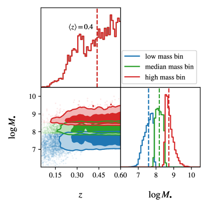
Figure 1: Joint and marginalised redshift and black-hole mass distribution of the type I samples. Low, median, and high black-hole mass bins are shown in blue, green, and red, respectively. We use the redshift-distribution weights $w_{\rm l,nofz}$ and the lensing efficiency weights $(\overline{\Sigma^{-1}_{\textrm{cr}}})^{2}$ for the 1D and 2D distributions.

2.1.1 SDSS type I AGNs

Based on the SDSS DR16 quasar catalog (Lyke et al., 2020), Wu & Shen fitted the spectrum of $750,414$ quasars in the redshift range $0.1<z<6$ and measured virial black-hole masses. As an update to Shen et al. (2011), they used the FWHM of H$\beta$, Mg II, and C IV broad emission lines (combined with the broad-line-region radius inferred from continuum luminosity) for their estimates. Here, we adopt their black-hole masses based on $H\beta$. The mean statistical error in $\log M_{\bullet}$ is much smaller than the systematic error of the virial black-hole mass ($\sim 0.4$ dex, see Shen, 2013).

As a complement to Wu & Shen (2022) at low black-hole masses, we use the AGN catalog from Liu et al. (2019), a complete AGN sample including both quasars and Seyfert galaxies from SDSS DR7. Black-hole masses are measured with H$\alpha$ and H$\beta$, and we adopt the $H\beta$ mass. This catalog contains $14,584$ AGNs at $z<0.35$.

We merge the two catalogs and remove duplicate objects. As a consistency check, we compare the fiducial black-hole mass of duplicate objects from both catalogs and find no significant systematic bias. In this work, we use AGNs with redshifts $0.05<z<0.6$ in the overlapping sky region between SDSS and UNIONS, resulting in $14,649$ lenses, three times larger than the sample size of previous type I AGN weak lensing studies (Luo et al., 2022). We divide the sample into low ($\log M_{\bullet}/M_{\odot}<7.9$), median ($7.9<\log M_{\bullet}/M_{\odot}<8.5$) and high ($\log M_{\bullet}/M_{\odot}>8.5$) black-hole mass bins. We introduce a weight $w_{\rm l,nofz}$ such that the weighted redshift distributions of the low and median mass bins equal the high-mass bin. This allows for a fair comparison between the mass bins free of redshift evolution or selection biases. The weighted distributions of the three bins are shown in Fig. 1.

2.1.2 SDSS type II AGNs

In addition to the type I catalog, we construct a type II AGN sample from the SDSS DR7 MPA-JHU catalog (Kauffmann et al., 2003; Brinchmann et al., 2004). We identify galaxies classified as AGNs using the BPT diagram (Baldwin et al., 1981) within the catalog. We estimate black-hole masses from the velocity dispersion using the $M_{\bullet}$-$\sigma_{*}$ relation proposed by Saglia et al. (2016). To correct for the aperture effect of velocity dispersion, we adopt the method outlined by Cappellari et al. (2006): First, we cross-match the sample with the NYU-VAGC catalog (Blanton et al., 2005) to obtain the $r$-band effective radius $R_{\rm e}$. Subsequently, we compute the aperture-corrected velocity dispersion, $\sigma_{*}$, using the formula $\sigma_{*}=\sigma_{\rm ap}(R_{\rm e}/R_{\rm ap}/8)^{-0.066}$, where $\sigma_{\rm ap}$ is the fiber velocity dispersion, and $R_{\rm ap}=3\arcsec$ is the fiber aperture for SDSS spectra. Finally, we restrict the sample to $21,532$ AGNs within the redshift range $z\in[0,0.2]$, black-hole mass range $\log M_{\bullet}/M_{\odot}\in[6.67,9.33]$, and falling in the UNIONS footprint. The type II sample exhibits lower redshifts ($\langle z\rangle\simeq 0.1$) than the type I sample.

2.2 Source sample

The shape catalogs serving as the background source sample in this work are the v1.3 ShapePipe and v1.0 lensfit catalogs of UNIONS. UNIONS is an ongoing multi-band wide-field imaging survey conducted with three telescopes (Canada-France-Hawai’i Telescope for $u$ and $r$ bands, Subaru telescope for $g$ and $z$ bands, and Pan-STARRS for the $i$ band) in Hawai’i. UNIONS will cover $4,800$ square degrees of the Northern sky with deep exposures and high-quality images. The depth (limiting magnitude with point source 5-sigma in a $2\arcsec$ diameter aperture) reaches $24.3$, $25.2$, $24.9$, $24.3$, and $24.1$ in $u,r,g,i$ and $z$, respectively.

At the time when the shear catalogs were produced (beginning of 2022), the survey covered an area of around $3,500$ square degrees in the $r$-band (the galaxy shapes were measured in this band). We did not have photometric redshifts for each source galaxy in the catalog at this stage of the UNIONS processing since the observations and calibration of the multi-band photometry are still ongoing. Instead, we estimated the overall redshift distribution by a method based on self-organizing maps. See Appendix A for more details about photometric redshifts.

The ShapePipe catalog was processed with the ShapePipe software package (Farrens et al., 2022). It contains $98$ million galaxies over an area of $3,200$ square degrees effective area. An earlier version of the ShapePipe catalog was published in Guinot et al. (2022). Some updates in processing were implemented for the v1.3 shear catalog used here, as follows. First, to model the PSF, instead of PSFEx (Bertin, 2011) we used MCCD (Liaudat et al., 2021) that performs a non-parametric Multi-CCD fit of the PSF over the entire focal plane. Second, we reduced the minimum area to detect an object from $10$ to $3$ pixels via the SExtractor configuration keyword DETECT_MINAREA = 3. This leads to a smaller galaxy selection bias on the ensemble shear estimates. Third, we added the section on the relative size between galaxies, $T_{\textrm{gal}}$, and the PSF, $T_{\textrm{PSF}}$, as $T_{\textrm{gal}}/T_{\textrm{PSF}}<3$ to avoid contamination by very diffuse, mostly low-signal-to-noise objects which tend to be artefacts.

The lensfit shape catalog was created with the THELI processing and lensfit software (Miller et al., 2007). It contains $109$ million galaxies in a $2,100$ square degree sky area. The effective area and number density of the ShapePipe and lensfit catalogs are different due to masking and processing choices. In the following, we use the more conservative lensfit mask for both shape catalogs, defining the common UNIONS footprint in which SDSS AGNs are selected. Both lensfit and ShapePipe catalogs are based on the same image data.

3 Methods

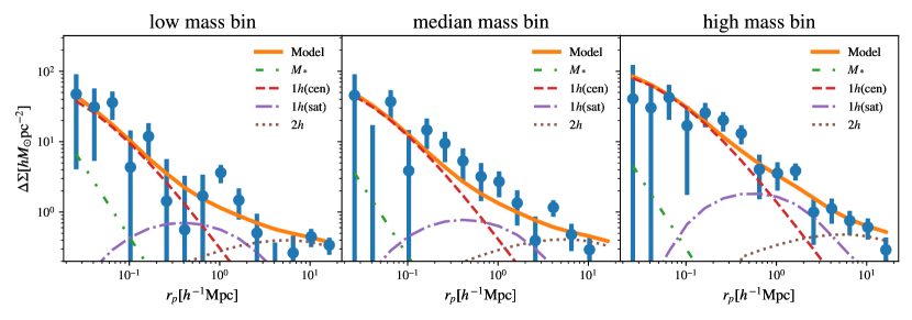
Figure 2: Galaxy-galaxy lensing excess surface mass density of three black-hole mass bins from ShapePipe. The best-fit HOD models are presented in orange lines. The baryon contribution, one-halo term of centrals, one-halo term of satellites, and two-halo term are plotted in green, red dashed, purple dash-dotted, and brown dotted lines, respectively. The measurements from the lensfit catalog are similar.

3.1 Galaxy-galaxy lensing technique

Galaxy-galaxy lensing denotes the shape distortions of background source galaxies due to the gravitational field of matter associated with foreground lens galaxies (see for a review Kilbinger, 2015). The main physical quantity related to galaxy-galaxy lensing is the excess surface density (ESD), $\Delta\Sigma$, at a projected distance $R$, defined as the mean surface density within a disk of radius $R$ minus a boundary term, which is the mean surface mass at radius $R$,

$$\Delta\Sigma(R)=\bar{\Sigma}(<R)-\Sigma(R).$$ (1)

The main observable for galaxy-galaxy lensing is the tangential shear, $\gamma_{\textrm{t}}$, of a source sample induced by a lens at projected distance $R$. This observable is related to the ESD via

$$\Delta\Sigma(R)=\Sigma_{\textrm{cr}}\gamma_{\textrm{t}}(R),$$ (2)

where the critical surface mass density $\Sigma_{\textrm{cr}}$ is defined as

$$\Sigma_{\textrm{cr}}(z_{\textrm{l}},z_{\textrm{s}})=\frac{c^{2}}{4\pi G}\frac{d(z_{\textrm{s}})}{d(z_{\textrm{l}})\,d(z_{\textrm{l}},z_{\textrm{s}})}\frac{1}{(1+z_{\textrm{l}})^{2}}.$$ (3)

Here, $z_{\textrm{s}}$ ($z_{\textrm{l}}$) is the source (lens) redshift, and $d(z_{\textrm{s}})$, $d(z_{\textrm{l}})$, and $d(z_{\textrm{l}},z_{\textrm{s}})$ are the angular diameter distance from the observer to the source, to the lens, and the lens-source distance, respectively. The constants are the speed of light $c$ and the Newtonian gravitational constant $G$.

3.2 Estimators

An estimator for the tangential shear of a background source sample around a lens galaxy population is

$$\left\langle\gamma_{\textrm{t}}(R)\right\rangle=\frac{\sum_{\rm ls}w_{\rm l}w_{\rm s}\epsilon_{\rm t,s}1_{b(R)}(|\vec{r}_{\rm l}-\vec{r}_{\rm s}|)}{\sum_{\rm ls}w_{\rm l}w_{\rm s}}.$$ (4)

This estimator is a weighted sum over the observed tangential ellipticities, $\epsilon_{\rm t,s}$, of source galaxies around lens galaxies. Source galaxies have a weight, $w_{\rm s}$, stemming from the galaxy shape estimation that indicates measurement uncertainties. Lens weights, $w_{\rm l}\equiv w_{\rm l,nofz}$, are introduced to homogenize the redshift distribution across lens samples as discussed in Sect. 2.2. The indicator function $1_{S}(x)$ of the set $S$ is unity if $x\in S$ and zero otherwise. In the above equation, this function selects galaxy pairs in a bin $b(R)$ around the projected separation $R$ of the pair; the shape of the function $b$ is chosen to be logarithmic.

Since we do not have photometric redshifts of individual background galaxies in the shape catalog, we compute an effective surface mass density by averaging Eq. (3) over the source redshift distribution. Inserting this effective value into Eq. (2) results in an average excess surface mass density. Since we cannot select sources to be strictly behind the lens sample, this leads to a divergence of $\Sigma_{\rm cr}$ when $z_{\textrm{s}}\to z_{\textrm{l}}$. A practical solution is to compute the inverse effective critical surface mass density,

$$\overline{\Sigma^{-1}_{\textrm{cr}}}(z_{\textrm{l}})=\frac{4\pi G}{c^{2}}\,d(z_{\textrm{l}})(1+z_{\textrm{l}}^{2})\,\int_{0}^{z_{\textrm{lim}}}\textrm{d}z_{\textrm{s}}\,n(z_{\textrm{s}})\,\frac{\,d(z_{\textrm{l}},z_{\textrm{s}})}{d(z_{\textrm{s}})}.$$ (5)

This quantity is the inverse of the critical surface mass density $\Sigma_{\textrm{cr}}$, Eq. (3), weighted by the source redshift distribution (see Sect. 2). The effective excess surface mass density is then

$$\overline{\Delta\Sigma}(R)=\gamma_{\textrm{t}}\left[\overline{\Sigma^{-1}_{\textrm{cr}}}(z_{\textrm{l}})\right]^{-1}.$$ (6)

Using Eq. (5), a first estimator for the excess surface mass density is readily derived as

$$\left\langle\Delta\Sigma(R)\right\rangle^{\prime}=\frac{\sum_{\rm ls}w_{\rm l}w_{\rm s}\epsilon_{\rm t,s}\left[\overline{\Sigma^{-1}_{\textrm{cr}}}(z_{\textrm{l}})\right]^{-1}1_{b(R)}(|\vec{r}_{\rm l}-\vec{r}_{\rm s}|)}{\sum_{\rm ls}w_{\rm l}w_{\rm s}}.$$ (7)

When using the effective surface mass density, the weights for a given lens can be updated by multiplication with the square of the inverse effective critical surface mass density Eq. (3), to down-weigh lenses with a low lensing efficiency, $w_{l}\to w_{\rm l}\left(\overline{\Sigma_{\textrm{cr}}^{-1}}(z_{\rm l})\right)^{2}$. With this, we write our final estimator of the excess surface mass density as

$$\left\langle\Delta\Sigma(R)\right\rangle=\frac{\sum_{\rm ls}w_{\rm l}\,\overline{\Sigma_{\textrm{cr}}^{-1}}(z_{\rm l})\,w_{\rm s}\,\epsilon_{\rm t,s}1_{b(R)}(|\vec{r}_{\rm l}-\vec{r}_{\rm s}|)}{\sum_{\rm ls}w_{\rm l}w_{\rm s}\left(\overline{\Sigma_{\textrm{cr}}^{-1}}(z_{\rm l})\right)^{2}}.$$ (8)

We also conduct a series of systematic tests and apply the boost factor correction $\left\langle\Delta\Sigma(R)^{\textrm{c}}\right\rangle=B(R)\left\langle\Delta\Sigma(R)\right\rangle$. We refer to Appendix B for details.

3.3 AGN lens model

Our lens sample contains both central and satellite AGN host galaxies, and we need to consider contributions to the excess surface density from both. We adopt a HOD model from Guzik & Seljak (2002) to describe the average ESD around the AGN sample,

$$\Delta\Sigma=\Delta\Sigma_{\rm b}+(1-f_{\rm sat})\Delta\Sigma_{\rm h,cen}+f_{\rm sat}\Delta\Sigma_{\rm h,sat}+\Delta\Sigma_{2\mathrm{h}},$$ (9)

where $f_{\rm sat}$ is the satellite galaxy fraction of the sample, left as a free parameter. $\Delta\Sigma_{\rm b}$ is the contribution from baryons in the host galaxy, containing the stellar mass $M_{*}$. $\Delta\Sigma_{\rm h,cen}$ and $\Delta\Sigma_{\rm h,sat}$ are the one-halo terms of the central and satellite galaxy, respectively. $\Delta\Sigma_{2\mathrm{h}}$ is the two-halo term. The terms are described in Appendix C in detail.

4 Results and Discussion

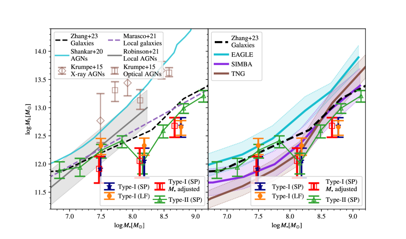
Figure 3: Black-Hole-to-Halo Mass Relation. In both panels, the dark blue stars and orange-filled circles are our type I results from the ShapePipe and lensfit catalogs, respectively. The blank red squares are type I ShapePipe results with an adjustment on BH mass. Blank green triangles correspond to the type II results with ShapePipe. Left Panel: Comparison with observational results from the literature. Brown squares and rhombuses are AGN clustering results for optically selected and X-ray selected samples from Krumpe et al. (2015), respectively. Cyan and grey lines show AGN clustering and dynamics results from Shankar et al. (2020) and Robinson et al. (2021), respectively. Results for normal galaxies are shown as dashed lines (purple line from Marasco et al. (2021) and black line from Zhang et al. (2023c)). Right Panel: Results from EAGLE, TNG, and SIMBA hydro-simulations are shown in cyan, brown, and purple lines with the $16-84$ percentiles displayed as shaded areas.

4.1 AGN black-hole-to-halo mass relation

The measured galaxy-galaxy lensing ESD profiles for the type I sample are shown in Fig. 2. We measure the ESD with a high signal-to-noise ratio (SNR) from ShapePipe (lensfit), with values of $24$ ($34$), $26$ ($36$), and $31$ ($41$) in the three bins, respectively. Our measurements are well reproduced by the HOD models with three free parameters. The amplitude of the ESD increases with $M_{\bullet}$, indicating that more massive SMBHs are situated in more massive halos. A similar trend is observed in the type II sample.

Fig. 3 shows the $M_{\bullet}$ - $M_{\textrm{h}}$ relation. Systematic errors in the shape measurements contribute to the total error budget at a comparable level to statistical errors, as indicated by the disparity between the type I ShapePipe and lensfit results. This underscores the robustness of our analysis across different shape catalogs.

We observe that more massive AGNs inhabit larger dark-matter halos, consistent with previous findings from dynamical (Robinson et al., 2021) and clustering analyses (Krumpe et al., 2015; Shankar et al., 2020). Robinson et al. (2021) employed reverberation mapping to determine black-hole masses and utilized HI FWHM to estimate halo masses for $24$ local AGNs. Our results are consistent with Robinson et al. (2021) at low masses but at $\log M_{\bullet}/M_{\odot}\simeq 8$, we find a lower halo mass. Our measured halo masses in the high-mass regime for both type I and type II samples are also systematically lower than the clustering results reported in Krumpe et al. (2015) and Shankar et al. (2020). The discrepancy between clustering and lensing halo masses was noticed in previous works (Mandelbaum et al., 2009). The clustering method leverages the monotonic relation between halo mass and halo bias, while weak lensing directly probes the matter overdensity around the tracers. It has long been known that the clustering strength of halos also depends on their secondary properties, such as the halo structure and the halo assembly history, which is called the halo assembly bias or the secondary halo bias (Gao & White, 2007; Wang et al., 2024). Therefore, if the host galaxies of AGNs prefer to live in dark-matter halos with biased secondary properties, it will alter the clustering strength without changing the host halo mass, while lensing is free of this effect.

In our results, both type I and type II samples exhibit similar $M_{\bullet}$-$M_{\rm h}$ relations despite their distinct classifications and redshift ranges. At higher black-hole masses, type I AGNs have a lower halo mass compared to type II. This difference may be interpreted as a systematic error in virial black-hole mass estimation. Recent spectroscopic interferometer measurements (GRAVITY Collaboration et al., 2024) of the AGN size-luminosity relation, upon which the virial mass measurement of type I AGNs relies, exhibit a significantly lower slope than the one proposed by Bentz et al. (2006) from reverberation mapping. Our type I black-hole masses are calculated by Wu & Shen (2022) using the H$\beta$ prescription from Vestergaard & Peterson (2006), which is based on Bentz et al. (2006). To account for the new measurements of (GRAVITY Collaboration et al., 2024), we use their size-luminosity slope to derive a black-hole mass prescription with the same sample and the same method as Vestergaard & Peterson (2006) and get the updated relation

$$\begin{split}\log\left(\frac{M_{\bullet}}{M_{\odot}}\right)=6.88&+2\log\left(\frac{\text{FWHM}_{\text{H}\beta}}{1000\,\text{km s}^{-1}}\right)\\ &+0.30\log\left(\frac{\lambda L_{\text{5100}}}{10^{44}\,\text{erg s}^{-1}}\right),\end{split}$$ (10)

where $\log{\lambda L_{\text{5100}}}$ is the luminosity of the continuum at $5100\text{\AA}$. We then adjust the average black-hole mass of the type I sample, as shown in Fig. 3. The black-hole mass of the high-mass bin changes the most, and moves the black-hole-halo-mass relation closer to the type II line. In conclusion, we find no evidence of type- or redshift-dependence in the $M_{\bullet}$-$M_{\rm h}$ relationship.

Furthermore, we compare our results to those of normal (non-AGN) galaxies. Marasco et al. (2021) measured halo masses through globular cluster dynamics and galaxy rotation curves in 55 nearby galaxies with directly measured black-hole masses. Zhang et al. (2023c) used the Dark Energy Camera Legacy Survey (Dey et al., 2019, DECaLS) shape catalog (Zhang et al., 2022) to measure galaxy-galaxy lensing of quiescent galaxies for $z<0.2$ for different $\sigma_{*}$ bins. We plot their result with black-hole masses inferred from the $M_{\bullet}$-$\sigma_{*}$ relation of Saglia et al. (2016). Compared to these results, we find that both type I and type II are broadly consistent with normal galaxies, suggesting no intrinsic difference in the $M_{\bullet}$-$M_{\rm h}$ relation between non-AGN galaxies and AGNs.

4.2 Constraint on black-hole mass in simulations

In state-of-the-art cosmological hydro-dynamical simulations, black-hole growth fed by gas accretion is a crucial factor in driving AGN feedback, which, in turn, is a major mechanism to suppress star formation activities in massive galaxies (Davé et al., 2019). However, these simulations cannot resolve the detailed accretion process. Instead, empirical subgrid recipes are employed to model this process, and the free parameters in these recipes need to be calibrated using observational scaling relations, such as the $M_{\bullet}$-$M_{*}$ relation (Habouzit et al., 2021).

However, we note that stellar mass itself is subject to several subgrid processes, including the stellar feedback and the AGN feedback, which makes the calibration process quite complicated. In contrast, halo masses are relatively robust and less sensitive to baryonic processes. Therefore, the black-hole-to-halo mass relation is a better scaling relation to calibration subgrid parameters in these simulations, and our work takes the first step to establish this relation in observation.

To compare our measurements with simulations, we used the RefL0100N1054 run for EAGLE (Schaye et al., 2015), the TNG100 run for IllustrisTNG (Springel et al., 2017), and the m100n1024 run for SIMBA (Davé et al., 2019). We calculated AGN luminosity from Eq. 1 in Habouzit et al. (2021) and selected central subhalos with $L_{\rm BH}/L_{\rm Edd}>0.001$ as the “AGN” sample in the simulation. We used the snapshot with $z\sim 0.4$, which is the average redshift of our type I AGN sample. We find no significant evolution between $z=0.4$ and $z=0.1$ in the three simulations, which is consistent with our observation. We also compared the “AGN” sample and central galaxy sample in the simulation and found no statistically significant difference between their $M_{\bullet}$-$M_{\rm h}$ relations. The AGN $M_{\bullet}$-$M_{\rm h}$ relations from the three simulations are plotted in the right panel of Fig. 3.

Although the three simulations calibrate their models to be in good agreement with observed relations (McConnell & Ma, 2013; Kormendy & Ho, 2013) between $M_{\bullet}$ and stellar mass of the galaxy, $M_{*}$, or of the bulge, $M_{\rm bulge}$, their $M_{\bullet}$-$M_{\rm h}$ relations do not perfectly match our measurements. The difference among the simulations under similar calibration clearly reflects how different black-hole accretion and AGN feedback mechanisms shape the black-hole masses in simulations. The predicted halo mass from EAGLE is consistent with ours at low masses but is significantly higher than ours at $\log M_{\bullet}/M_{\odot}>8$. However, TNG and SIMBA predict lower halo masses at fixed black-hole masses compared to EAGLE, which are more consistent with our observations (both type I and type II). Among the three simulations, SIMBA has the $M_{\bullet}$-$M_{\rm h}$ relation that is the closest to ours, with all differences within one sigma.

4.3 Future prospects

Current data suffers from a small AGN sample size and limited accuracy of black-hole mass estimation. Large spectroscopic surveys such as DESI (Levi et al., 2013) and PFS will provide larger quasar samples with reliable virial black-hole mass measurements. Already now integral field spectroscopy and reverberation mapping observations are improving the virial black-hole mass measurement accuracy. From the perspective of weak-lensing data, we will soon get the $4,800$ square degrees shape catalog with photo-$z$s from the completed UNIONS survey.

Future weak-lensing surveys such as Euclid (Euclid Collaboration et al., 2020), Rubin-LSST (Željko Ivezić et al., 2019), Roman (Spergel et al., 2015), CSST (Gong et al., 2019), and WFST (WFST Collaboration et al., 2023), will provide galaxy samples with accurate shape measurements to higher redshifts, covering larger sky areas. This will enable us to measure the $M_{\bullet}$-$M_{\rm h}$ relation with higher accuracy, as well as its dependency on the host galaxy properties.

Appendix A Estimation of the redshift distribution

From UNIONS $r$-band observations, we follow three steps to estimate the redshift distribution of our weak-lensing source sample. The first step is assigning multi-band photometry to UNIONS galaxies. Using the overlap of UNIONS $r$-band observations with the CFHTLenS (Canada-France-Hawaii Telescope Lensing Survey; Heymans et al., 2012; Erben et al., 2013) W3 field ($\sim 44.2$ sq. deg), we assign $ugriz$ magnitudes by cross-matching. This can be done since CFHTLenS has deeper photometry (Hildebrandt et al., 2012) than UNIONS, basically all CFIS (UNIONS $r$-band) objects are also visible in CFHTLenS, and the underlying redshift distribution is assumed to be the same after matching.

We calibrate the redshifts distribution with spectroscopic calibration samples which are constructed from DEEP2 (DEEP2 Galaxy Redshift Survey; Newman et al., 2013), VVDS (VIMOS VLT Deep Survey; Le Fèvre et al., 2005), and VIPERS (VIMOS Public Extragalactic Redshift Survey; Scodeggio et al., 2018). These surveys are also observed with CFHTLenS $ugriz$ photometry. With the multi-band photometry of the spectroscopic sample, we then train self-organising maps (SOM; Kohonen, 1982; Masters et al., 2015) to organise the sample in high dimensional magnitude space. The SOM splits the matched sample into subsamples in its so-called SOM cells. The initial SOM cell grid has a resolution of 101 $\times$ 101 cells and is then hierarchically clustered into $5,000$ resolution elements for reliable statistics lateron, shown in Fig. 4. We then populate the SOM with the UNIONS weak lensing sources with $ugriz$ photometry.

For every SOM cell $i$, a weight $w_{i}^{\mathrm{SOM}}$ is defined, which is the ratio of the number of UNIONS objects (weighted by their shape weights) over the number of spectroscopic objects (Wright et al., 2020). Finally, we get the UNIONS $p(z)$ by re-weighting the spectroscopic redshift distribution $p^{\rm spec}(z)$ according to the weights $w_{i}^{\mathrm{SOM}}$ in the $i$’th SOM cells (Wright et al., 2020),

$$p(z)=\int w^{\mathrm{SOM}}(z)p^{\rm spec}(z)\mathrm{d}z=\sum w_{i}^{\mathrm{SOM}}p_{i}^{\mathrm{spec}}(z),$$ (A1)

where $p_{i}^{\mathrm{spec}}(z)$ is the histogram of spectroscopic objects per SOM cell $i$. $p^{\rm Spec}(z)$ and $p(z)$ are shown in Fig. 4.

Figure 4: In panel (a), the trained SOM coloured by the counts of the spectroscopic sample is shown. In panel (b), the blinded redshift distributions $p^{\rm spec}(z)$ and $p(z)$ are plotted with green and purple bars, respectively.

Appendix B Systematic Tests for Galaxy-galaxy Lensing Measurements

To validate our galaxy-galaxy lensing measurement, we conducted two null tests and measured the boost factor.

B.1 Cross-shear ($\Delta\Sigma_{\times}$) test

Weak gravitational lensing does not produce shape distortions in the cross direction, therefore the cross component of the shear $\gamma_{\times}$ or “cross excess surface density” $\Delta\Sigma_{\times}$ is expected to be zero in the absence of systematics. Thus, $\Delta\Sigma_{\times}$ can be interpreted as a null test of systematics in the lensing measurement process. We measure $\Delta\Sigma_{\times}$ with the same method and sample as for $\Delta\Sigma$,

$$\left\langle\Delta\Sigma(R)^{w}_{\times}\right\rangle =\frac{\sum_{\rm ls}w_{\rm l}\,\overline{\Sigma_{\textrm{cr}}^{-1}}(z_{\rm l})\,w_{\rm s}\,\epsilon_{\times,{\rm s}}1_{b(R)}(|\vec{r}_{\rm l}-\vec{r}_{\rm s}|)}{\sum_{\rm ls}w_{\rm l}w_{\rm s}\left(\overline{\Sigma_{\textrm{cr}}^{-1}}(z_{\rm l})\right)^{2}}.$$ (B1)

The results of the $\Delta\Sigma_{\times}$ test are shown in Fig. 5. All data points are consistent with zero at three sigma, and $\sim 70\%$ are zero within one sigma. No evidence is found of any significant systematic errors.

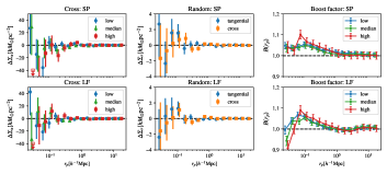
Figure 5: Systematic tests of lensing measurements. The top (bottom) column shows tests for ShapePipe (lensfit). The left two panels correspond to $\Delta\Sigma_{\rm x}$. Low-, median-, and high-mass bins of type I sample are shown in blue circles, green triangles, and red rectangles in each panel. The middle two panels show the excess surface density and cross excess surface density around a random sample. The right two panels present the boost factor of the type I sample. Low-, median-, and high-mass bins are shown in blue, green, and red points. In all panels, some results are slightly displaced in the $x$-direction to make the figure clear.

B.2 Random lens test

We also measure lensing signals around a random sample as a null test. This sample is constructed by randomly sampling the SDSS footprint and then selecting the sub-sample in the sky region overlapping with UNIONS. To match the redshift distribution, we randomly assign the redshifts of the high-mass bin lens sample (the other two bins have the same $p(z)$ after weighting) to the random sample. Our random sample contains $543,402$ “galaxies”.

Following the same procedure as before, we measure both tangential and cross components with respect to the random sample with the ShapePipe and lensfit shape catalogs. The results are presented in Fig. 5. The lensing signals are in good consistency with zero, indicating that systematic errors in the measurement are not significant.

B.3 Boost factor

Galaxy-galaxy lensing signals are diluted by galaxies physically associated with lens galaxies, whose shapes are not affected by lensing. Since we can not exclude these galaxies without photo-$z$s in this work, it is important to quantify this effect. With the same random sample as in the random lens test, we calculate the boost factor (Hirata et al., 2004), which is defined as $B(r)=(N_{\rm rs}\sum_{\rm ls}w_{\rm ls})/(N_{\rm ls}\sum_{\rm rs}w_{\rm rs})$, where $N_{\rm ls}$ and $N_{\rm rs}$ are the number of lens-source pairs and random-source pairs, respectively, and $w_{\rm ls}$ and $w_{\rm rs}$ are corresponding lensing weights. The results are shown in Fig. 5. We apply the boost factor correction to the lensing signals we use in this work.

Appendix C Details of the HOD model

C.1 Baryonic contribution

For source-lens separations (at the lens redshifts) that are much larger than the size of a typical galaxy, that galaxy can be considered as a point mass. The baryonic contribution to the excess surface density, which contains stars, dust and gas, can then be written as

$$\Delta\Sigma_{\textrm{b}}(R)=\frac{M_{*}}{\pi R^{2}}.$$ (C1)

C.2 One-halo central galaxy contribution

We adopt a Navarro-Frenk-White (NFW) model to describe the density profile of the host halo for central galaxies,

$$\rho(r)=\frac{\rho_{0}}{(r/r_{\textrm{s}})(1+r/r_{\textrm{s}})^{2}},$$ (C2)

with $\rho_{0}=200\,\rho_{\textrm{m}}/(3I_{c})$ and $I_{c}=c^{-3}\int_{0}^{c}\textrm{d}x\,x(1+x)^{-2}$. Here, $\rho_{\textrm{m}}$ is the mean density of the Universe, and $c$ is the halo concentration parameter, defined as the ratio between the virial radius $r_{200}$ and scale radius $r_{\textrm{s}}$ of the halo, $c=r_{200}/r_{\textrm{s}}$. Assuming that the halo center is located at the central galaxy, the excess surface density $\Delta\Sigma_{\rm NFW}$ of the halo within a disk of radius $R$ is

$$\Delta\Sigma_{\textrm{h,cen}}(R)=\Delta\Sigma_{\rm NFW}(R)=\bar{\Sigma}_{\rm NFW}(<R)-\Sigma_{\rm NFW}(R)=\frac{M_{\rm h}}{2\pi r_{\textrm{s}}^{2}I}\left[g(R/r_{\textrm{s}})-f(R/r_{\textrm{s}})\right],$$ (C3)

where $M_{\rm h}$ is the halo mass. The functions $f(x)$ and $g(x)$ are defined as

$$f(x)=\left\{\begin{array}[]{lr}\frac{1}{x^{2}-2}\left[1-\frac{\ln[(1+\sqrt{1-x^{2}})/x]}{\sqrt{1-x^{2}}}\right],&x<1\\ \frac{1}{3},&x=1\\ \frac{1}{x^{2}-1}\left[1-\frac{\arctan(\sqrt{x^{2}-1})}{\sqrt{x^{2}-1}}\right];&x>1\end{array}\right.,\qquad g(x)=\left\{\begin{array}[]{lr}\frac{2}{x^{2}}\left[\ln{x/2}+\frac{\ln[(1+\sqrt{1-x^{2}})/x]}{\sqrt{1-x^{2}}}\right],&x<1\\ 2-2\ln 2,&x=1\\ \frac{2}{x^{2}}\left[\ln{x/2}+\frac{\arctan(\sqrt{x^{2}-1})}{\sqrt{x^{2}-1}}\right],&x>1\end{array}\right..$$ (C4)

C.3 One-halo satellite galaxy contribution

We use the NFW model also for the host halo of satellites. Compared to the central-galaxy term, the satellite halo has a spatial offset. First, the excesses surface density given the projected distance between the satellite galaxy and the halo center, $R_{\textrm{sat}}$, is

$$\Delta\Sigma_{\rm off}(R|M_{\rm h,sat},R_{\rm sat})=\frac{1}{2\pi}\int_{0}^{2\pi}\Delta\Sigma_{\rm NFW}\left((R^{2}+R_{\rm sat}^{2}+2RR_{\rm sat}\cos\theta)^{\frac{1}{2}}|M_{\rm h,sat}\right)\textrm{d}\theta.$$ (C5)

We integrate this equation over the distribution functions of $M_{\rm h,sat}$ and $R_{\rm sat}$ to obtain the effective one-halo satellite term as

$$\Delta\Sigma_{\rm h,sat}(R)=\iint\Delta\Sigma_{\rm off}(R|M_{\rm h,sat},R_{\rm sat})P(R_{\rm sat}|M_{\rm h,sat})P(M_{\rm h,sat})\textrm{d}R_{\rm sat}\textrm{d}M_{\rm h,sat}$$ (C6)

We assume that satellite galaxies follow the spatial distribution of dark matter, which is the NFW density profile. We set

$$P(R_{\rm sat}|M_{\rm h,sat})\propto\Sigma_{\rm NFW}(R_{\rm sat},M_{\rm h,sat})\cdot 2\pi R_{\rm sat}\textrm{d}R_{\rm sat}=\frac{M_{\rm h,sat}}{2\pi r_{\textrm{s}}^{2}(M_{\rm h,sat})I}f[R_{\rm sat}/r_{\textrm{s}}(M_{\rm h,sat})]\cdot 2\pi R_{\rm sat}\textrm{d}R_{\rm sat}.$$ (C7)

Following Guzik & Seljak (2002), we use a halo occupation distribution (HOD) model to infer

$$P(M_{\rm h,sat}|M_{\rm sub})\propto P(M_{\rm sub}|M_{\rm h,sat})P(M_{\rm h,sat})\propto\langle N_{\rm sat}(M_{\rm h,sat})\rangle F_{\rm h}(M_{\rm h,sat}),$$ (C8)

where $F_{\rm h}(M_{\rm h})$ is halo mass function and $\langle N_{\rm sat}(M_{\rm h})\rangle$ is the halo occupation function of satellite galaxies. In this work, we use the halo mass function from Tinker et al. (2008) and the HOD model from Guzik & Seljak (2002).

C.3.1 Two-halo term

For the two-halo term, we use the Tinker et al. (2010) halo bias model to infer the halo-matter correlation function $\xi_{\rm hm}=b_{\rm h}\xi_{\rm mm}$ based on the dark-matter correlation function $\xi_{\rm mm}$. From that, we can calculate the surface density as

$$\Sigma_{\rm 2h}(R)=b_{\rm h}(M_{\rm h,cen})\times 2\bar{\rho}\int_{R}^{\infty}\xi_{\rm mm}(r)\frac{r\textrm{d}r}{\sqrt{r^{2}-R^{2}}}.$$ (C9)

C.4 Lens model validation

To validate the model, we cross-match the type II sample with the Yang et al. (2007) SDSS group catalog to select a purely central-galaxy subsample. Subsequently, we measure the ESD for both the type II sample and the central-galaxy subsample using the ShapePipe catalog. Next, we fit the central-galaxy subsample lensing signals with the lens model (Sect. 3.3), but set the satellite fraction to zero. This allows us to make two consistency tests. First, we compare the contributions of central galaxies from the entire type II sample by using the best-fit central ESD term to the ESD measured from the central-galaxy subsample. We find that they are broadly consistent. Second, we compare the inferred halo masses. They are consistent within one sigma across all mass ranges considered in this work, indicating that our lens model is reliable.

References

- Baes et al. (2003) Baes, M., Buyle, P., Hau, G. K. T., & Dejonghe, H. 2003, MNRAS, 341, L44, doi: 10.1046/j.1365-8711.2003.06680.x
- Baldwin et al. (1981) Baldwin, J. A., Phillips, M. M., & Terlevich, R. 1981, PASP, 93, 5, doi: 10.1086/130766
- Bandara et al. (2009) Bandara, K., Crampton, D., & Simard, L. 2009, ApJ, 704, 1135, doi: 10.1088/0004-637X/704/2/1135
- Bentz et al. (2006) Bentz, M. C., Peterson, B. M., Pogge, R. W., Vestergaard, M., & Onken, C. A. 2006, ApJ, 644, 133, doi: 10.1086/503537
- Bertin (2011) Bertin, E. 2011, in Astronomical Society of the Pacific Conference Series, Vol. 442, Astronomical Data Analysis Software and Systems XX, ed. I. N. Evans, A. Accomazzi, D. J. Mink, & A. H. Rots, 435
- Blanton et al. (2005) Blanton, M. R., Schlegel, D. J., Strauss, M. A., et al. 2005, AJ, 129, 2562, doi: 10.1086/429803
- Brinchmann et al. (2004) Brinchmann, J., Charlot, S., White, S. D. M., et al. 2004, MNRAS, 351, 1151, doi: 10.1111/j.1365-2966.2004.07881.x
- Cappellari et al. (2006) Cappellari, M., Bacon, R., Bureau, M., et al. 2006, MNRAS, 366, 1126, doi: 10.1111/j.1365-2966.2005.09981.x
- Davé et al. (2019) Davé, R., Anglés-Alcázar, D., Narayanan, D., et al. 2019, MNRAS, 486, 2827, doi: 10.1093/mnras/stz937
- Davis et al. (2019) Davis, B. L., Graham, A. W., & Combes, F. 2019, ApJ, 877, 64, doi: 10.3847/1538-4357/ab1aa4
- Dey et al. (2019) Dey, A., Schlegel, D. J., Lang, D., et al. 2019, AJ, 157, 168, doi: 10.3847/1538-3881/ab089d
- Dressler & Richstone (1988) Dressler, A., & Richstone, D. O. 1988, The Astrophysical Journal, 324, 701, doi: 10.1086/165930
- Erben et al. (2013) Erben, T., Hildebrandt, H., Miller, L., et al. 2013, MNRAS, 433, 2545, doi: 10.1093/mnras/stt928
- Euclid Collaboration et al. (2020) Euclid Collaboration, Blanchard, A., Camera, S., et al. 2020, A&A, 642, A191, doi: 10.1051/0004-6361/202038071
- Farrens et al. (2022) Farrens, S., Guinot, A., Kilbinger, M., et al. 2022, A&A, 664, A141, doi: 10.1051/0004-6361/202243970
- Ferrarese (2002) Ferrarese, L. 2002, ApJ, 578, 90, doi: 10.1086/342308
- Ferrarese & Merritt (2000) Ferrarese, L., & Merritt, D. 2000, ApJ, 539, L9, doi: 10.1086/312838
- Gao & White (2007) Gao, L., & White, S. D. M. 2007, MNRAS, 377, L5, doi: 10.1111/j.1745-3933.2007.00292.x
- Gebhardt et al. (2000) Gebhardt, K., Bender, R., Bower, G., et al. 2000, ApJ, 539, L13, doi: 10.1086/312840
- Gong et al. (2019) Gong, Y., Liu, X., Cao, Y., et al. 2019, ApJ, 883, 203, doi: 10.3847/1538-4357/ab391e
- GRAVITY Collaboration et al. (2024) GRAVITY Collaboration, Amorim, A., Bourdarot, G., et al. 2024, arXiv e-prints, arXiv:2401.07676, doi: 10.48550/arXiv.2401.07676
- Guinot et al. (2022) Guinot, A., Kilbinger, M., Farrens, S., et al. 2022, A&A, 666, A162, doi: 10.1051/0004-6361/202141847
- Guzik & Seljak (2002) Guzik, J., & Seljak, U. 2002, MNRAS, 335, 311, doi: 10.1046/j.1365-8711.2002.05591.x
- Habouzit et al. (2021) Habouzit, M., Li, Y., Somerville, R. S., et al. 2021, MNRAS, 503, 1940, doi: 10.1093/mnras/stab496
- Heymans et al. (2012) Heymans, C., Van Waerbeke, L., Miller, L., et al. 2012, MNRAS, 427, 146, doi: 10.1111/j.1365-2966.2012.21952.x
- Hildebrandt et al. (2012) Hildebrandt, H., Erben, T., Kuijken, K., et al. 2012, MNRAS, 421, 2355, doi: 10.1111/j.1365-2966.2012.20468.x
- Hirata et al. (2004) Hirata, C. M., Mandelbaum, R., Seljak, U., et al. 2004, MNRAS, 353, 529, doi: 10.1111/j.1365-2966.2004.08090.x
- Kauffmann et al. (2003) Kauffmann, G., Heckman, T. M., White, S. D. M., et al. 2003, MNRAS, 341, 33, doi: 10.1046/j.1365-8711.2003.06291.x
- Kilbinger (2015) Kilbinger, M. 2015, Reports on Progress in Physics, 78, 086901, doi: 10.1088/0034-4885/78/8/086901
- Kohonen (1982) Kohonen, T. 1982, Biological cybernetics, 43, 59
- Kormendy & Bender (2011) Kormendy, J., & Bender, R. 2011, Nature, 469, 377, doi: 10.1038/nature09695
- Kormendy & Ho (2013) Kormendy, J., & Ho, L. C. 2013, Annual Review of Astronomy and Astrophysics, 51, 511, doi: 10.1146/annurev-astro-082708-101811
- Kormendy & Ho (2013) Kormendy, J., & Ho, L. C. 2013, ARA&A, 51, 511, doi: 10.1146/annurev-astro-082708-101811
- Kormendy & Richstone (1995) Kormendy, J., & Richstone, D. 1995, ARA&A, 33, 581, doi: 10.1146/annurev.aa.33.090195.003053
- Krumpe et al. (2015) Krumpe, M., Miyaji, T., Husemann, B., et al. 2015, ApJ, 815, 21, doi: 10.1088/0004-637X/815/1/21
- Krumpe et al. (2023) Krumpe, M., Miyaji, T., Georgakakis, A., et al. 2023, The spatial clustering of ROSAT all-sky survey Active Galactic Nuclei: V. The evolution of broad-line AGN clustering properties in the last 6 Gyr. https://arxiv.org/abs/2304.02036
- Le Fèvre et al. (2005) Le Fèvre, O., Vettolani, G., Garilli, B., et al. 2005, A&A, 439, 845, doi: 10.1051/0004-6361:20041960
- Leauthaud et al. (2015) Leauthaud, A., J. Benson, A., Civano, F., et al. 2015, MNRAS, 446, 1874, doi: 10.1093/mnras/stu2210
- Levi et al. (2013) Levi, M., Bebek, C., Beers, T., et al. 2013, arXiv e-prints, arXiv:1308.0847, doi: 10.48550/arXiv.1308.0847
- Liaudat et al. (2021) Liaudat, T., Bonnin, J., Starck, J.-L., et al. 2021, A&A, 646, A27, doi: 10.1051/0004-6361/202039584
- Liu et al. (2019) Liu, H.-Y., Liu, W.-J., Dong, X.-B., et al. 2019, ApJS, 243, 21, doi: 10.3847/1538-4365/ab298b
- Luo et al. (2018) Luo, W., Yang, X., Lu, T., et al. 2018, ApJ, 862, 4, doi: 10.3847/1538-4357/aacaf1
- Luo et al. (2022) Luo, W., Silverman, J. D., More, S., et al. 2022, arXiv e-prints, arXiv:2204.03817, doi: 10.48550/arXiv.2204.03817
- Lyke et al. (2020) Lyke, B. W., Higley, A. N., McLane, J. N., et al. 2020, The Astrophysical Journal Supplement Series, 250, 8, doi: 10.3847/1538-4365/aba623
- Magorrian et al. (1998) Magorrian, J., Tremaine, S., Richstone, D., et al. 1998, AJ, 115, 2285, doi: 10.1086/300353
- Mandelbaum et al. (2009) Mandelbaum, R., Li, C., Kauffmann, G., & White, S. D. M. 2009, MNRAS, 393, 377, doi: 10.1111/j.1365-2966.2008.14235.x
- Mandelbaum et al. (2006) Mandelbaum, R., Seljak, U., Kauffmann, G., Hirata, C. M., & Brinkmann, J. 2006, MNRAS, 368, 715, doi: 10.1111/j.1365-2966.2006.10156.x
- Marasco et al. (2021) Marasco, A., Cresci, G., Posti, L., et al. 2021, MNRAS, 507, 4274, doi: 10.1093/mnras/stab2317
- Masters et al. (2015) Masters, D., Capak, P., Stern, D., et al. 2015, ApJ, 813, 53, doi: 10.1088/0004-637X/813/1/53
- McConnell & Ma (2013) McConnell, N. J., & Ma, C.-P. 2013, ApJ, 764, 184, doi: 10.1088/0004-637X/764/2/184
- Miller et al. (2007) Miller, L., Kitching, T. D., Heymans, C., Heavens, A. F., & van Waerbeke, L. 2007, MNRAS, 382, 315, doi: 10.1111/j.1365-2966.2007.12363.x
- Newman et al. (2013) Newman, J. A., Cooper, M. C., Davis, M., et al. 2013, ApJS, 208, 5, doi: 10.1088/0067-0049/208/1/5
- Pizzella et al. (2005) Pizzella, A., Corsini, E. M., Dalla Bontà, E., et al. 2005, ApJ, 631, 785, doi: 10.1086/430513
- Planck Collaboration et al. (2020) Planck Collaboration, Aghanim, N., Akrami, Y., et al. 2020, A&A, 641, A6, doi: 10.1051/0004-6361/201833910
- Powell et al. (2018) Powell, M. C., Cappelluti, N., Urry, C. M., et al. 2018, ApJ, 858, 110, doi: 10.3847/1538-4357/aabd7f
- Powell et al. (2022) Powell, M. C., Allen, S. W., Caglar, T., et al. 2022, arXiv e-prints, arXiv:2209.02728. https://arxiv.org/abs/2209.02728
- Robinson et al. (2021) Robinson, J. H., Bentz, M. C., Courtois, H. M., et al. 2021, ApJ, 912, 160, doi: 10.3847/1538-4357/abedaa
- Sabra et al. (2015) Sabra, B. M., Saliba, C., Akl, M. A., & Chahine, G. 2015, The Astrophysical Journal, 803, 5, doi: 10.1088/0004-637X/803/1/5
- Saglia et al. (2016) Saglia, R. P., Opitsch, M., Erwin, P., et al. 2016, ApJ, 818, 47, doi: 10.3847/0004-637X/818/1/47
- Schaye et al. (2015) Schaye, J., Crain, R. A., Bower, R. G., et al. 2015, MNRAS, 446, 521, doi: 10.1093/mnras/stu2058
- Scodeggio et al. (2018) Scodeggio, M., Guzzo, L., Garilli, B., et al. 2018, A&A, 609, A84, doi: 10.1051/0004-6361/201630114
- Shankar et al. (2020) Shankar, F., Allevato, V., Bernardi, M., et al. 2020, Nature Astronomy, 4, 282, doi: 10.1038/s41550-019-0949-y
- Shen (2013) Shen, Y. 2013, Bulletin of the Astronomical Society of India, 41, 61, doi: 10.48550/arXiv.1302.2643
- Shen et al. (2011) Shen, Y., Richards, G. T., Strauss, M. A., et al. 2011, ApJS, 194, 45, doi: 10.1088/0067-0049/194/2/45
- Shimasaku & Izumi (2019) Shimasaku, K., & Izumi, T. 2019, The Astrophysical Journal Letters, 872, L29, doi: 10.3847/2041-8213/ab053f
- Spergel et al. (2015) Spergel, D., Gehrels, N., Baltay, C., et al. 2015, arXiv e-prints, arXiv:1503.03757, doi: 10.48550/arXiv.1503.03757
- Springel et al. (2017) Springel, V., Pakmor, R., Pillepich, A., et al. 2017, Monthly Notices of the Royal Astronomical Society, 475, 676, doi: 10.1093/mnras/stx3304
- Tinker et al. (2008) Tinker, J., Kravtsov, A. V., Klypin, A., et al. 2008, ApJ, 688, 709, doi: 10.1086/591439
- Tinker et al. (2010) Tinker, J. L., Robertson, B. E., Kravtsov, A. V., et al. 2010, ApJ, 724, 878, doi: 10.1088/0004-637X/724/2/878
- Vestergaard & Peterson (2006) Vestergaard, M., & Peterson, B. M. 2006, ApJ, 641, 689, doi: 10.1086/500572
- Volonteri et al. (2011) Volonteri, M., Natarajan, P., & Gültekin, K. 2011, ApJ, 737, 50, doi: 10.1088/0004-637X/737/2/50
- Wang et al. (2024) Wang, K., Mo, H. J., Chen, Y., et al. 2024, MNRAS, 528, 2046, doi: 10.1093/mnras/stae163
- Wechsler & Tinker (2018) Wechsler, R. H., & Tinker, J. L. 2018, Annual Review of Astronomy and Astrophysics, 56, 435, doi: 10.1146/annurev-astro-081817-051756
- WFST Collaboration et al. (2023) WFST Collaboration, Wang, T., Liu, G., et al. 2023, arXiv e-prints, arXiv:2306.07590, doi: 10.48550/arXiv.2306.07590
- Wright et al. (2020) Wright, A. H., Hildebrandt, H., van den Busch, J. L., & Heymans, C. 2020, A&A, 637, A100, doi: 10.1051/0004-6361/201936782
- Wu & Shen (2022) Wu, Q., & Shen, Y. 2022, ApJS, 263, 42, doi: 10.3847/1538-4365/ac9ead
- Yang et al. (2008) Yang, X., Mo, H. J., & van den Bosch, F. C. 2008, ApJ, 676, 248, doi: 10.1086/528954
- Yang et al. (2007) Yang, X., Mo, H. J., van den Bosch, F. C., et al. 2007, ApJ, 671, 153, doi: 10.1086/522027
- Zhang et al. (2023a) Zhang, H., Behroozi, P., Volonteri, M., et al. 2023a, arXiv e-prints, arXiv:2305.19315, doi: 10.48550/arXiv.2305.19315
- Zhang et al. (2023b) —. 2023b, MNRAS, 518, 2123, doi: 10.1093/mnras/stac2633
- Zhang et al. (2022) Zhang, J., Liu, C., Vaquero, P. A., et al. 2022, AJ, 164, 128, doi: 10.3847/1538-3881/ac84d8
- Zhang et al. (2023c) Zhang, Z., Wang, H., Luo, W., et al. 2023c, arXiv e-prints, arXiv:2305.06803, doi: 10.48550/arXiv.2305.06803
- Željko Ivezić et al. (2019) Željko Ivezić, Kahn, S. M., Tyson, J. A., et al. 2019, The Astrophysical Journal, 873, 111, doi: 10.3847/1538-4357/ab042c