Conformalized Credal Set Predictors

Abstract

Credal sets are sets of probability distributions that are considered as candidates for an imprecisely known ground-truth distribution. In machine learning, they have recently attracted attention as an appealing formalism for uncertainty representation, in particular due to their ability to represent both the aleatoric and epistemic uncertainty in a prediction. However, the design of methods for learning credal set predictors remains a challenging problem. In this paper, we make use of conformal prediction for this purpose. More specifically, we propose a method for predicting credal sets in the classification task, given training data labeled by probability distributions. Since our method inherits the coverage guarantees of conformal prediction, our conformal credal sets are guaranteed to be valid with high probability (without any assumptions on model or distribution). We demonstrate the applicability of our method to natural language inference, a highly ambiguous natural language task where it is common to obtain multiple annotations per example.

Keywords Conformal Prediction  $\cdot$ Uncertainty Representation  $\cdot$ Credal Sets

1 Introduction

Representing and quantifying uncertainty is becoming increasingly important in machine learning (ML), particularly as ML models are employed in safety-critical application domains such as medicine or autonomous driving. In such domains, a distinction between so-called aleatoric uncertainty and epistemic uncertainty is often useful (Hora, 1996). Broadly speaking, aleatoric uncertainty is due to the inherent randomness of the data-generating process, whereas epistemic uncertainty stems from the learner’s lack of knowledge about the best predictive model. Thus, while the former is irreducible, the latter can in principle be reduced through additional information, e.g., by gathering additional data to learn from.

Representation of aleatoric and epistemic uncertainty requires formalism more expressive than standard probability distributions (Hüllermeier and Waegeman, 2021). One such formalism which prevails in the recent ML literature is second-order probability distributions. Essentially, in a classification setting, these are distributions over distributions over classes. Models producing second-order distributions as predictions can be learned in a classical Bayesian way (Kendall and Gal, 2017; Depeweg et al., 2018) or using more recent approaches such as evidential deep learning (Sensoy et al., 2018). Yet, approaches of that kind are not unproblematic and have been subject to criticism (Bengs et al., 2022, 2023). Another formalism suitable for representing both types of uncertainty is the concept of a credal set, which is well-established in the field of imprecise probability theory (Walley, 1991) and meanwhile also attracted attention in ML (Shaker and Hüllermeier, 2020; Hüllermeier et al., 2022). Credal sets are (convex) sets of probability distributions that can be considered as candidates for an imprecisely known ground-truth distribution. Figure 1 shows examples of credal sets in a three-class scenario, where the space of distributions can be visualized by the two-dimensional probability simplex. Broadly speaking, the larger the credal set, the higher the epistemic uncertainty, and the more “in the middle” the set is located, i.e., the closer it is to the uniform distribution, the higher the aleatoric uncertainty.

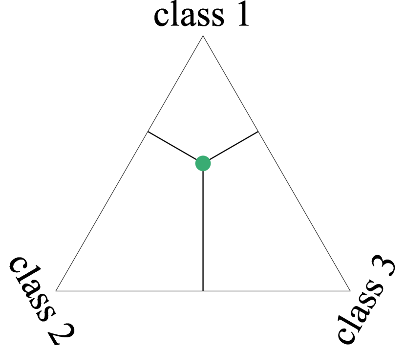
Figure 1: For the three-class classification setting, the space of probability distributions can be illustrated by a two-dimensional simplex: each point in the simplex corresponds to a probability distribution so that credal sets can be depicted as regions. The left case corresponds to the special case of a singleton (credal) set, i.e., a precise probability distribution, signifying aleatoric but no epistemic uncertainty. The case in the middle represents partial knowledge with a certain degree of (epistemic) uncertainty about the true distribution, and the right one corresponds to the case of complete ignorance, where nothing is known about the distribution.

Premise a child is on the ground crying. Hypothesis A child on the ground crying as others look on. True dist. $[0.06,0.94,0.00]$

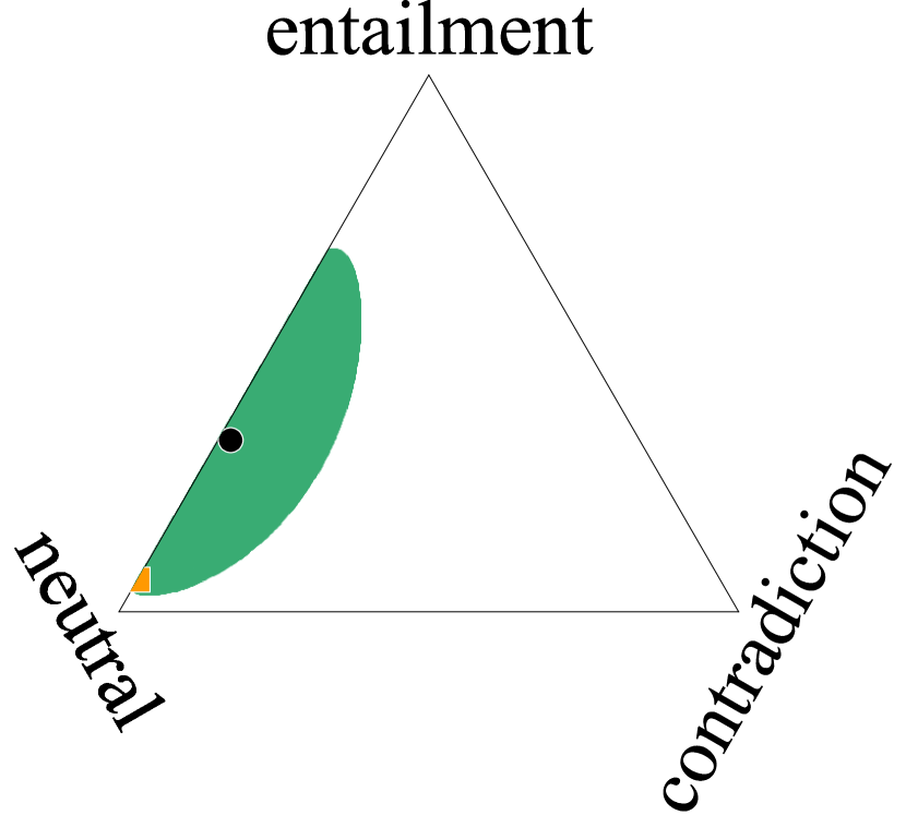
Premise uh-huh and is it true i mean is it um Hypothesis It is absolutely correct. True dist. $[0.31,0.52,0.17]$

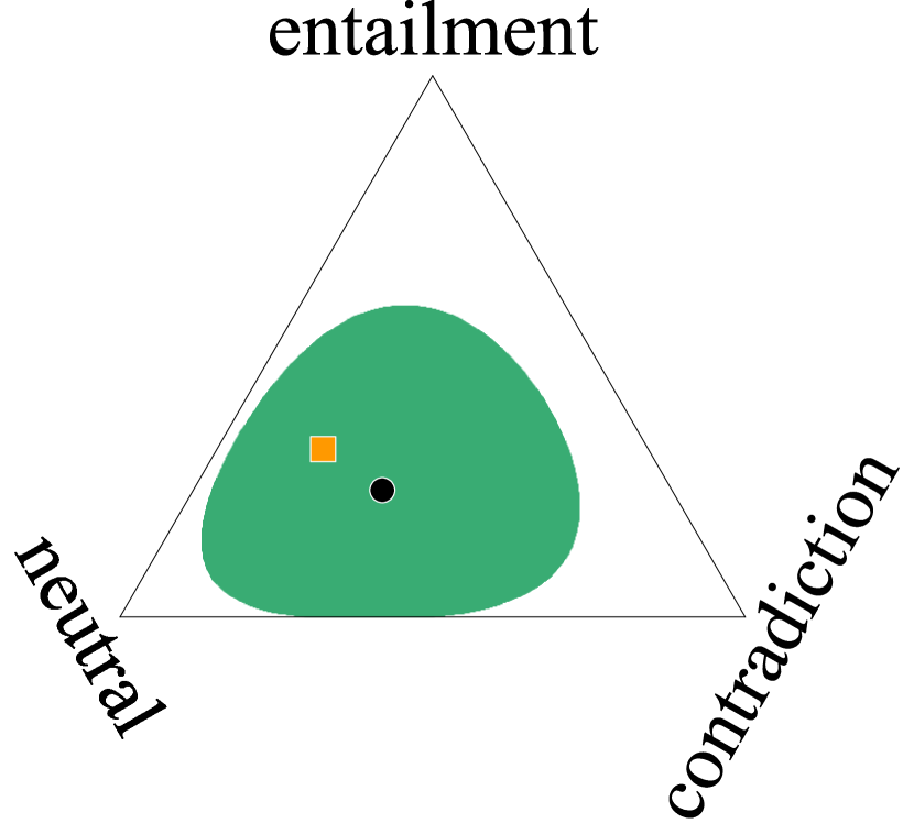
Figure 2: An illustration of our proposed conformalized credal sets on two instances from the ChaosNLI dataset (Nie et al., 2020). Green regions indicate credal sets, while the true and the predicted distributions are marked with orange squares and black circles, respectively.

Learning to predict second-order representations, such as credal sets or second-order distributions, from standard “zero-order” supervised data — training instances together with observed class labels — is a difficult endeavor. For the case of second-order probabilities, it is even provably impossible to predict uncertainty in an “unbiased” way, i.e., without imposing strong prior assumptions on the epistemic uncertainty (Bengs et al., 2022, 2023). In this paper, we assume “first-order” training data, i.e., instances associated with probability distributions over the class labels. In other words, instances are labeled probabilistically instead of being assigned a deterministic class label. Obviously, this type of data facilitates second-order learning. Not less importantly, it is becoming increasingly available in practice, for example, in the form of aggregations over multiple annotations per data instance, and hence increasingly relevant in applications (Uma et al., 2022; Stutz et al., 2023b)

Our method leverages the framework of conformal prediction (CP), a non-parametric approach for set-valued prediction rooted in classical frequentist statistics (Vovk et al., 2022). Based on relatively mild assumptions, CP is able to provide theoretical guarantees in the form of marginal coverage: Predicted sets are guaranteed to cover the true target with high probability. Since our method inherits these coverage guarantees, our conformal credal sets are guaranteed to be valid with high probability (without any assumptions on model or distribution).

Our main contribution is the proposal of a novel, conformal method to construct credal set predictors from first-order training data:

• We propose a CP based method to construct conformal credal sets. To this end, we make use of two types of nonconformity functions based on distance resp. likelihood, and leveraging first-order resp. second-order probability predictors.

• On ChaosNLI (Nie et al., 2020), a very ambiguous natural language inference task with multiple annotations per example, we show that our conformal credal sets are indeed valid, i.e., include the true ground truth distribution with high probability (see Figure 2 for an illustration). We also compare the efficiency of predictions (size of the predicted sets) for different nonconformity functions.

• We complement this study with controlled experiments on synthetic data, specifically investigating the performance of credal set prediction in the presence of label noise.

2 Related Work

Credal sets are widely used as models for representing uncertainty, notably within the domain of imprecise probabilities (Walley, 1991). As already mentioned, they can represent both types of uncertainty, aleatoric and epistemic. In the context of data analysis and statistical inference, credal sets are often used as robust models of prior information, namely for modeling imprecise information about the prior in Bayesian inference (Walley, 1996).

In machine learning, credal sets have been used for generalizing some of the standard methods, including naive Bayes (Zaffalon, 2002; Corani and Zaffalon, 2008), Bayesian networks (Corani et al., 2012), and decision trees (Abellán and Moral, 2003). Typically, these approaches generalize simple frequentist inference to robust Bayesian inference, making use of an imprecise version of the Dirichlet model (a conjugate prior for the multinomial distribution). Compared to our approach, these methods are learning on standard (zero-order) training data. Moreover, despite representing uncertainty in predictions, they do not provide any formal guarantees.

Conformal prediction (Vovk et al., 2022), briefly introduced in Section 3.2 below, has recently gained attention for various applications in machine learning, especially for classification tasks (Sadinle et al., 2019; Romano et al., 2020; Angelopoulos et al., 2020; Stutz et al., 2021; Fisch et al., 2022). These methods mostly focus on split conformal prediction using a held-out calibration set (Papadopoulos et al., 2002), overcoming computational limitations of earlier transductive or bagging approaches (Vovk et al., 2022; Vovk, 2015; Steinberger and Leeb, 2016; Barber et al., 2021; Linusson et al., 2020). While tackling classification tasks, our method for constructing conformal credal sets has more similarity with conformal regression (Romano et al., 2019; Sesia and Romano, 2021), particularly in multivariate settings (Dietterich and Hostetler, 2022), as we essentially conformalize the simplex space of categorical distributions. Our conformity scores differ, however, in that they are specific for distributions rather than considering general multivariate spaces. This work also relates to work on appropriate measures of inefficiency (Vovk et al., 2017) as measuring the inefficiency of our conformal credal sets is non-trivial. Most closely related to our work is the recent work by Stutz et al. (2023b), who consider conformal prediction in settings with high aleatoric uncertainty. However, we explicitly target the construction of conformal credal sets, while Stutz et al. (2023b) mainly focus on constructing confidence sets of classes.

First-order data. In settings with high aleatoric uncertainty, labeling each example with a single, unique class is clearly insufficient. In practice, this is typically captured by high disagreement among annotators – a problem particularly common in natural language tasks (Reidsma and op den Akker, 2008; Aroyo and Welty, 2014, 2015; Schaekermann et al., 2016; Dumitrache et al., 2019; Pavlick and Kwiatkowski, 2019; Röttger et al., 2022; Abercrombie et al., 2023). Handling this disagreement has received considerable attention lately (Uma et al., 2021) as it offers to go beyond this zero-order information. For example, recent work on evaluation with disagreeing annotators (Stutz et al., 2023a) argues the use of these annotations to get approximate first-order information for evaluation. This approach is becoming more and more viable with crowdsourcing tools (Kovashka et al., 2016; Sorokin and Forsyth, 2008; Snow et al., 2008) being an integral component of the benchmark, making multiple annotations per data instance more accessible. We follow a similar approach in our construction of conformal credal sets.

3 Background

3.1 Supervised Learning and Predictive Uncertainty

We consider the setting of (polychotomous) classification with label space $\mathcal{Y}=\{1,\ldots,K\}$ and an instance space $\mathcal{X}$. As usual, we assume an underlying data-generating process in the form of a probability distribution $P$ on $\mathcal{X}\times\mathcal{Y}$, so that observations $(X,Y)$ are i.i.d. samples from $P$. We denote by $\boldsymbol{\lambda}^{\boldsymbol{x}}\in\Delta^{K}$ the conditional probability distribution $P(\cdot\,|\,X=\boldsymbol{x})$, which we also consider as an element of the $(K-1)$-simplex

$$\Delta^{K}:=\left\{\boldsymbol{\lambda}=(\lambda_{1},\ldots,\lambda_{K})^{\top}\,|\,\lambda_{k}\geq 0,\|\boldsymbol{\lambda}\|_{1}=1\right\}\subset\mathbb{R}^{K}\,.$$

Thus, for each class label $k\in\mathcal{Y}$, the probability to observe $Y=k$ as an outcome for $\boldsymbol{x}\in\mathcal{X}$ is given by $\lambda^{\boldsymbol{x}}_{k}$.

Since the dependency between instances $X$ and outcomes $Y$ is non-deterministic, the prediction of $Y$ given $X=\boldsymbol{x}$ is necessarily afflicted with uncertainty, even if the ground-truth distribution $\boldsymbol{\lambda}^{\boldsymbol{x}}$ is known. As already said, this uncertainty is commonly referred to as aleatoric (Hüllermeier and Waegeman, 2021). Intuitively, the closer $\boldsymbol{\lambda}^{\boldsymbol{x}}$ to the uniform distribution $\boldsymbol{p}_{\text{uni}}=(1/K,\ldots,1/K)^{\top}$, the higher the uncertainty, and the closer it is to a degenerate (Dirac) distribution assigning all probability mass to a single class (a corner point in $\Delta^{K}$), the lower the uncertainty. Various measures have been proposed to quantify this uncertainty in numerical terms, with Shannon entropy as the arguably best-known representative (Depeweg et al., 2018).

Instead of assuming $\boldsymbol{\lambda}^{\boldsymbol{x}}$ to be known, suppose now that only a prediction $\hat{\boldsymbol{\lambda}}^{\boldsymbol{x}}$ of this distribution is available. Epistemic uncertainty refers to the uncertainty about how well the latter approximates the former, and hence to the additional uncertainty in the prediction of outcome $Y$ that is caused by the discrepancy between $\hat{\boldsymbol{\lambda}}^{\boldsymbol{x}}$ and the ground-truth $\boldsymbol{\lambda}^{\boldsymbol{x}}$. We seek to capture this discrepancy by means of credal sets

$$Q\in\mathcal{Q}_{K}\subset\Delta^{K}\,,$$

with the idea that $Q\ni\boldsymbol{\lambda}^{\boldsymbol{x}}$ holds with high probability. Typically, credal sets are assumed to be convex, and further restrictions might be imposed on $\mathcal{Q}_{K}$ for practical and computational reasons, for example, a restriction to convex polygons (with a finite number of extreme points).

3.2 Conformal Prediction

Conformal prediction provides a general framework for producing set-valued predictions with a certain guarantee of validity. In a supervised setting, consider data points of the form $Z=(X,U)\in\mathcal{X}\times\mathcal{U}$, and the task is to predict $U$ given $X=\boldsymbol{x}$. We assume the space $Z$ to be equipped with a nonconformity measure $f:\,\mathcal{Z}\longrightarrow\mathbb{R}$ that quantifies the “strangeness” of $\boldsymbol{z}$, i.e., the higher $f(\boldsymbol{z})$, the less normal or expected the data point. Let $\mathcal{D}_{\text{calib}}\subset\mathcal{Z}$ be a (randomly generated) set of data points, called calibration data, and $Z$ another data point that remains unobserved. Under the assumption of exchangeability, i.e., that the calibration data and the query point $Z$ have been generated by an exchangeable process, we want to construct a so-called confidence set $C\subseteq\mathcal{U}$ that guarantees coverage:

$$\mathbb{P}(U\in C)\geq 1-\alpha.$$ (1)

By a simple combinatorial argument (Vovk et al., 2022), the confidence set $C$ can be constructed as

$$C(\boldsymbol{x}):=\big{\{}\,u\in\mathcal{U}\,|\,f(\boldsymbol{x},u)<q(\mathcal{E},\alpha^{\prime})\,\big{\}}\,,$$ (2)

where $\alpha^{\prime}=|\mathcal{E}|^{-1}\lceil(1+|\mathcal{E}|)(1-\alpha)\rceil$, and $q(\mathcal{E};\alpha^{\prime})$ denotes the $\alpha^{\prime}$-quantile of $\mathcal{E}$.

Importantly, the guarantee (2) holds regardless of the nonconformity function $f(\cdot)$, which, however, has an influence on the efficiency of the prediction: The more appropriate the function, the smaller the prediction set $C$ tends to be. Normally, $f(\cdot)$ is not predefined but constructed in a data-driven way using training data $\mathcal{D}_{\text{train}}$. For example, a common approach is to train a predictor $\pi:\,\mathcal{X}\longrightarrow\mathcal{U}$ and then define $f(\boldsymbol{x},u)$ in terms of $d(u,\pi(\boldsymbol{x}))$, where $d(\cdot,\cdot)$ is an appropriate distance function on $\mathcal{U}$. Replacing the point-prediction $\pi(\boldsymbol{x})\in\mathcal{U}$ by the prediction set $C(\boldsymbol{x})\subset\mathcal{U}$ can then be seen as “conformalizing” the predictor $\pi$: Using the calibration data, CP estimates a high-probability upper bound on the distance between point-predictions and actual outcomes, and corrects the former correspondingly.

4 Conformal Credal Set Prediction

Recall the setting and notation from Section 3.1. Our goal is to learn a credal set predictor $h:\,\mathcal{X}\longrightarrow\mathcal{Q}_{K}$, that is, a model that makes predictions in the form of credal sets, thereby representing both aleatoric and epistemic uncertainty. To this end, we assume probabilistic training data of the form

$$\mathcal{D}=\left\{\big{(}\boldsymbol{x}_{1},\boldsymbol{\lambda}^{\boldsymbol{x}_{1}}\big{)},\ldots,\big{(}\boldsymbol{x}_{N},\boldsymbol{\lambda}^{\boldsymbol{x}_{N}}\big{)}\right\}\subset\mathcal{X}\times\Delta^{K}\,.$$ (3)

The model $h$ should be able to predict the (probabilistic) outcomes for new query instances in a reliable way. More specifically, suppose that $\boldsymbol{x}_{\text{new}}$ is a new query instance (following the same distribution as the training data) for which a prediction is sought. The credal prediction $Q=h(\boldsymbol{x}_{\text{new}})$ should then be valid in the sense that $Q\ni\boldsymbol{\lambda}^{\boldsymbol{x}_{\text{new}}}$ with high probability. At the same time, the prediction should be informative in the sense that the (epistemic) uncertainty reflected by $Q$ is as small as possible. Again, various measures for quantifying the latter can be found in the literature (Klir and Wierman, 1999; Sale et al., 2023).

We aim to construct the credal set predictor $h$ by means of (inductive) conformal prediction. Following the conformalization recipe outlined in Section 3.2, we partition $\mathcal{D}$ into $\mathcal{D}_{\text{train}}$ and $\mathcal{D}_{\text{calib}}$, using the former for model training and the latter for calibration. Regarding the training step, we explore two learning strategies, connected with two ways of defining a nonconformity function, which is pivotal in the calibration step.

The first approach is based on training a standard (first-order) probability predictor, i.e., a probabilistic classifier $g:\,\mathcal{X}\longrightarrow\Delta^{K}$ that maps instances to the (first-order) probability distribution on $\mathcal{Y}$. This can be achieved, for example, by minimizing the cross-entropy loss between the ground truth and the predicted distributions, i.e.,

$$g=\operatornamewithlimits{argmin}_{\bar{g}\in\mathcal{H}}\sum_{(\boldsymbol{x}_{i},\boldsymbol{\lambda}^{\boldsymbol{x}_{i}})\in\mathcal{D}_{\text{train}}}-\sum_{k=1}^{K}\lambda^{\boldsymbol{x}_{i}}_{k}\log(\bar{g}(\boldsymbol{x}_{i})_{k}),$$

where $\mathcal{H}$ is a hypothesis space. Given a predictor $g(\cdot)$ of this kind, nonconformity is naturally defined in terms of distance:

$$f_{1}(\boldsymbol{x},\boldsymbol{\lambda}^{\boldsymbol{x}}):=d(\boldsymbol{\lambda}^{\boldsymbol{x}},g(\boldsymbol{x}))\,,$$ (4)

where $d(\cdot,\cdot)$ is a suitable distance function on $\Delta^{K}$, such as total variation, Wasserstein distance, etc.

An alternative approach is motivated by recent work on (epistemic) uncertainty representation via second-order probability distributions. A second-order learner $G:\,\mathcal{X}\longrightarrow\mathbb{P}(\Delta^{K})$ maps each input $\boldsymbol{x}$ to a distribution over $\Delta^{K}$. Given the training data, meaningful learning in this context can be accomplished, for instance, by parameterizing the second-order distributions using Dirichlet distributions. Specifically, one can assume that each $\boldsymbol{x}$ is associated with a Dirichlet distribution characterized by the parameter vector $\boldsymbol{\theta}^{\boldsymbol{x}}\in\mathbb{R}^{K}_{+}$ with the probability density function

$$P(\boldsymbol{\lambda}\,|\,\boldsymbol{\theta}^{\boldsymbol{x}})=\frac{1}{B({\boldsymbol{\theta}^{\boldsymbol{x}}})}\prod_{k=1}^{K}\lambda_{k}^{\theta^{\boldsymbol{x}}_{k}-1}\,,$$ (5)

where $B(\cdot)$ is the multivariate beta function. This way, $\boldsymbol{\lambda}^{\boldsymbol{x}}$ can be thought of as a sample from that distribution, i.e., $\boldsymbol{\lambda}^{\boldsymbol{x}}\sim\text{Dir}(\boldsymbol{\theta}^{\boldsymbol{x}})$. Our model then essentially yields a prediction $\hat{\boldsymbol{\theta}}^{\boldsymbol{x}}$ of the true parameter $\boldsymbol{\theta}^{\boldsymbol{x}}$ for every $\boldsymbol{x}$, and its optimization involves minimizing the negative log-likelihood loss

$$\sum_{(\boldsymbol{x}_{i},\boldsymbol{\lambda}^{\boldsymbol{x}_{i}})\in\mathcal{D}_{\text{train}}}\bigg{(}\log(B(\hat{\boldsymbol{\theta}}^{\boldsymbol{x}_{i}}))-\sum_{k=1}^{K}(\hat{\theta}^{\boldsymbol{x}_{i}}_{k}-1)\log(\lambda^{\boldsymbol{x}_{i}}_{k})\bigg{)}.$$

Given a second-order predictor $\hat{\boldsymbol{\theta}}^{\boldsymbol{x}}$, nonconformity can be defined as a decreasing function of likelihood, e.g., as 1 minus relative likelihood:

$$f_{2}(\boldsymbol{x},\boldsymbol{\lambda}^{\boldsymbol{x}})=1-\frac{P(\boldsymbol{\lambda}^{\boldsymbol{x}}\,|\,\hat{\theta}^{\boldsymbol{x}})}{\max_{\boldsymbol{\lambda}\in\Delta^{K}}P(\boldsymbol{\lambda}\,|\,\hat{\theta}^{\boldsymbol{x}})}.$$ (6)

Using the nonconformity function $f_{i}(\cdot)$ ($i\in\{1,2\}$), we obtain the set of nonconformity scores by

$$\mathcal{E}_{i}:=\Big{\{}f_{i}(\boldsymbol{x}_{j},\boldsymbol{\lambda}^{\boldsymbol{x}_{j}})\,|\,(\boldsymbol{x}_{j},\boldsymbol{\lambda}^{\boldsymbol{x}_{j}})\in\mathcal{D}_{\text{calib}}\Big{\}}.$$ (7)

Accordingly, the credal set can be defined as

$$h_{i}(\boldsymbol{x}_{\text{new}}):=\big{\{}\,\boldsymbol{\lambda}\in\Delta^{K}\,|\,f_{i}(\boldsymbol{x}_{\text{new}},\boldsymbol{\lambda})<q(\mathcal{E}_{i},\alpha^{\prime})\,\big{\}}\,.$$ (8)

Algorithm 1 Conformal Credal Set Prediction

  Input:

  

• Data $\mathcal{D}$; error rate $\alpha$; query instance $\boldsymbol{x}_{\text{new}}$.

  Process:

  

• Partition $\mathcal{D}$ into $\mathcal{D}_{\text{train}}$ and $\mathcal{D}_{\text{calib}}$.

• Train a first-order ($i=1$) or a second-order ($i=2$) predictor using $\mathcal{D}_{\text{train}}$.

• Choose a nonconformity function $f_{i}$ as in (4) or (6) that suits the trained predictor to obtain the set of scores $\mathcal{E}_{i}$.

• Set $\alpha^{\prime}=|\mathcal{E}_{i}|^{-1}\lceil(1+|\mathcal{E}_{i}|)(1-\alpha)\rceil$.

  Output:

• $h_{i}(\boldsymbol{x}_{\text{new}})=\big{\{}\,\boldsymbol{\lambda}\in\Delta^{K}\,|\,f_{i}(\boldsymbol{x}_{\text{new}},\boldsymbol{\lambda})<q(\mathcal{E}_{i},\alpha^{\prime})\,\big{\}}\,.$

Algorithm 1 outlines a summary of the proposed methods. In the following theorem, we state the validity of the predicted set, that is, the restatement of the conformal coverage guarantee (Vovk et al., 2022) adjusted to our setting.

Theorem 4.1.

Let $\mathcal{P}$ denote the joint probability distribution on $(X,\Lambda)\in\mathcal{X}\times\Delta^{K}$. If data points in $\mathcal{D}_{\text{calib}}$ and $(\boldsymbol{x}_{\text{new}},\boldsymbol{\lambda}^{\boldsymbol{x}_{\text{new}}})$ are drawn i.i.d. (exchangeably) from $\mathcal{P}$, then the conformal credal sets in (8) are valid, i.e.,

$$\mathbb{P}\big{(}\boldsymbol{\lambda}^{\boldsymbol{x}_{\text{new}}}\in h_{i}(\boldsymbol{x}_{\text{new}})\big{)}\geq 1-\alpha\,,~{}\text{ for }i\in\{1,2\}.$$

4.1 Noisy Observations

So far, we (implicitly) assumed that ground-truth probability distributions $\boldsymbol{\lambda}^{\boldsymbol{x}_{i}}$ will be provided as training (and calibration) data. Needless to say, this assumption will rarely hold true in practice. Instead, observations will rather be noisy versions $\tilde{\boldsymbol{\lambda}}^{\boldsymbol{x}_{i}}$ of the true probabilities, i.e., the data will be of the form

$$\mathcal{D}=\left\{\big{(}\boldsymbol{x}_{1},\tilde{\boldsymbol{\lambda}}^{\boldsymbol{x}_{1}}\big{)},\ldots,\big{(}\boldsymbol{x}_{N},\tilde{\boldsymbol{\lambda}}^{\boldsymbol{x}_{N}}\big{)}\right\}\subset\mathcal{X}\times\Delta^{K}\,.$$ (9)

Notably, such datasets emerge in scenarios where each data instance $\boldsymbol{x}$ is annotated by multiple human experts, which recently have attracted a lot of attention in the context of machine learning and also conformal prediction (Stutz et al., 2023b; Javanmardi et al., 2023). In this context, $\tilde{\boldsymbol{\lambda}}^{\boldsymbol{x}}$ denotes the distribution derived from aggregating annotator disagreements concerning the label of instance ${\boldsymbol{x}}$. Of course, conformal prediction can still be applied to noisy data of that kind, but the coverage guarantee will then only hold for the noisy labeling:

$$\mathbb{P}\left(\tilde{\boldsymbol{\lambda}}^{\boldsymbol{x}_{\text{new}}}\in h(\boldsymbol{x}_{\text{new}})\right)\geq 1-\tilde{\alpha}.$$ (10)

Practically, one may expect that the guarantees will hold for the ground-truth as well, simply because calibration on noisy instead of clean data will tend to make prediction regions larger and hence more conservative. Moreover, since nonconformity is derived from a predictive model $g(\cdot)$ that seeks to recover ground-truth probabilities, the latter should conform at least as well as noisy distributions. Of course, this intuition is not a formal guarantee. In order to provide such a guarantee for the ground-truth probabilities, one obviously needs to make some assumptions. Concretely, let us make the following bounded noise assumption for the labeling process: The labeling noise is (stochastically) bounded in the sense that, given the nonconformity function $f$ and a (small) probability $\delta>0$, there exists a tolerance $\epsilon>0$ such that

$$\mathbb{P}\left(|f(\boldsymbol{x},\boldsymbol{\lambda}^{\boldsymbol{x}})-f(\boldsymbol{x},\tilde{\boldsymbol{\lambda}}^{\boldsymbol{x}})|<\epsilon\right)\geq 1-\delta$$ (11)

all $\boldsymbol{x}\in\mathcal{X}$.

Theorem 4.2.

Let $\alpha>0$ be any miscoverage rate, and suppose the bounded noise assumption holds. Let $q=q(\mathcal{E},\tilde{\alpha})$ be the critical threshold on the noisy calibration data $\mathcal{D}_{\text{calib}}$ for miscoverage rate

$$\tilde{\alpha}=\frac{\alpha-\delta}{1-\delta}\,.$$

Then, for any new query $\boldsymbol{x}_{\text{new}}\in\mathcal{X}$,

$$\mathbb{P}\big{(}f(\boldsymbol{x}_{\text{new}},{\boldsymbol{\lambda}}^{\boldsymbol{x}_{\text{new}}})<q+\epsilon\big{)}\geq 1-\alpha\,.$$

The proof is deferred to Appendix A.. As a consequence of this result, a conformal predictor learned on the noisy data with modified miscoverage rate $\tilde{\alpha}$ can be turned into a valid predictor (with miscoverage rate $\alpha$) for the ground-truth data by increasing the learned rejection threshold by $\epsilon$, provided the bounded noise property (11) can be ascertained. Thus, if we denote the corresponding credal set predictor by $h_{\epsilon}$, we can guarantee that

$$\mathbb{P}\big{(}\boldsymbol{\lambda}^{\boldsymbol{x}_{\text{new}}}\in h_{\epsilon}(\boldsymbol{x}_{\text{new}})\big{)}\geq 1-\alpha\,.$$ (12)

5 Experiments

In this section, we evaluate the performance of our proposed methods using both synthetic and real datasets. In vanilla conformal prediction, the performance of a method is usually assessed based on the average prediction set size, aka efficiency, and the average coverage on the test set. It is more appealing to have the promised coverage with smaller sets. In our scenario, the analytical calculation of credal sets is not feasible. Therefore, for the sake of illustration as well as other analyses, such as efficiency calculation, we resort to approximations. We discretize the simplex with a resolution of $0.005$, yielding $M=19969$ distributions. This enables the straightforward construction of credal sets, as defined in (8). The efficiency is gauged by considering the fraction of all $M$ distributions that lie within the predicted credal sets. All implementations and experiments can be found in the technical supplement of this work.

5.1 Learning Model

Table 1: Summary of the nonconformity functions used in experiments.

Name Formulation Predictor TV $\frac{1}{2}\sum_{k=1}^{K}|\lambda_{k}^{\boldsymbol{x}}-g(\boldsymbol{x})_{k}|$ first-order WS - first-order KL $\sum_{k=1}^{K}\lambda_{k}^{\boldsymbol{x}}\log(\frac{\lambda_{k}^{\boldsymbol{x}}}{g(\boldsymbol{x})_{k}})$ first-order Inner $1-\sum_{k=1}^{K}\lambda_{k}^{\boldsymbol{x}}g(\boldsymbol{x})_{k}$ first-order SO as in (6) second-order

In our experiments, we employ a deep neural network as the learner. Specifically, the model consists of three hidden layers with $256$, $64$, and $16$ units, utilizing ReLU as the activation function. Prior to the output layer, a dropout layer with a rate of $0.3$ is incorporated. The same model architecture serves both first- and second-order predictors, differing only in the activation functions of the output layers. For the first-order predictor, softmax is used, while for the second-order predictor, ReLU is employed. Learning is facilitated using the Adam optimizer with a learning rate of $10^{-4}$, utilizing cross-entropy as the loss function for the first-order predictor and negative log-likelihood for the second-order predictor.

5.2 Nonconformity Functions

CP should work regardless of the choice of nonconformity score function, while this choice can affect the efficiency and geometry of the prediction set. For the sake of comparison, we examine different nonconformity functions in our experiments. When utilizing a first-order predictor, besides total variation (TV) and the First Wasserstein (WS) distance, we also investigate the Kullback–Leibler (KL) divergence and 1 minus the inner product (Inner) as nonconformity functions. For the second-order predictor, we consider 1 minus the relative likelihood (SO) as defined in (6). Table 1 offers a summary of all five nonconformity functions employed in our experiments.

5.3 Real Data

We focus on the ChaosNLI dataset (Nie et al., 2020), an English Natural Language Inference (NLI) dataset that captures the inherent variability in human judgments of textual entailment. Here, the classes are entailment, neutral, and contradiction for each premise-hypothesis pair. Instances in this dataset are selected from the development sets of SNLI (Bowman et al., 2015), MNLI (Williams et al., 2018), and AbductiveNLI (Bhagavatula et al., 2019), for which the majority vote was less than three among the five human annotators. These instances were then given to $100$ independent humans for annotation, given strict annotation guidelines.

We combine the chaos-SNLI and chaos-MNLI subsets, resulting in a dataset of $3113$ datapoints. For model training, we leverage a language model from the Hugging Face transformers library (Wolf et al., 2019), initially trained on SNLI and MultiNLI datasets for classification tasks. We utilize the last hidden layer output of this model to embed the premise-hypothesis pairs from our $3113$ instances, serving as inputs for our deep neural network. To split the data, we randomly select $500$ instances for calibration, $500$ for testing, and the remaining for training. This process is repeated ten times with different random seeds. In Figure 3, we compare the resulting credal sets of different nonconformity functions for three specific instances. Figure 4 summarizes the overall performance of the proposed methods on this data under different miscoverage rates ($\alpha$). Notably, the mean of the average coverage over the test data across various random seeds aligns with or exceeds the nominal value, consistent with the conformal prediction guarantee.

Premise-Hypothesis pair	TV	KL	WS	Inner	SO
Premise: A man in a bar drinks from a pitcher while a man in a green hat looks on and a woman in a black shirt drink from a glass. Hypothesis: The women is drinking water.
	$0.24$	$0.18$	$0.28$	$0.36$	$0.06$
Premise: The streets are busy and people contemplate their futures. Hypothesis: People are screaming
	$0.33$	$0.20$	$0.33$	$0.41$	$0.47$
Premise: A photographer snaps a midair action shot of a snowboarder. Hypothesis: The midair shot snaps at a boarder of snow.
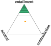
	$0.31$	$0.27$	$0.26$	$0.34$	$0.08$

Figure 3: Various credal sets obtained for three instances from ChaosNLI dataset (Nie et al., 2020). The ground truth distributions are denoted by orange squares. Black circles indicate model predictions in cases employing a first-order learner (first four columns). For the last column, utilizing a second-order learner, the predicted second-order distributions are represented through contour plots. The miscoverage rate is $\alpha=0.2$, and the efficiency of each credal set is written below it.

Figure 4: Coverage and efficiency results of different nonconformity functions applied on the ChaosNLI dataset (Nie et al., 2020). The horizontal dashed lines indicate the nominal coverage levels.

5.4 Synthetic Data

The primary objective of conducting experiments with synthetic data is to illustrate the impact of noisy observations, particularly to showcase the behavior of the proposed credal sets when we only have access to an approximation of the ground truth distributions. Our experiment revolves around a $K$-class classification task with $K\in\{3,4,6,8,10\}$. For each $K$, we consider $10$-dimensional features $X\in\mathbb{R}^{10}$, where each $X_{1},\ldots,X_{10}$ are independent standard normal random variables. Subsequently, we generate a random matrix $\beta\in\mathbb{R}^{10\times K}$, with its elements drawn independently from the standard normal distribution. To define the ground truth probability over the classes for object $X$, we use the following formulation:

$$\lambda_{k}^{\boldsymbol{x}}:=\mathbb{P}(Y=k|\boldsymbol{x})=\frac{Z_{j}(\boldsymbol{x})}{\sum_{j}Z_{j}(\boldsymbol{x})},$$

where $Z(\boldsymbol{x}):=\exp(\boldsymbol{x}^{\top}\beta)$. Employing this data-generating process, we generate $N=1500$ samples to construct the dataset $\mathcal{D}^{K}=\{(\boldsymbol{x}_{i},\boldsymbol{\lambda}^{\boldsymbol{x}_{i}})\}_{i=1}^{N}$.

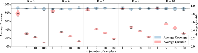
Figure 5: Coverage and quantile results for synthetic data, where the ground truth distributions are approximated by observing $m$ samples from them. The horizontal dashed line indicates the nominal coverage levels $1-\alpha=0.9$.

To obtain noisy versions of $\mathcal{D}^{K}$, we employ a sampling approach. Specifically, we independently sample each distribution $\boldsymbol{\lambda}^{\boldsymbol{x}_{i}}$ $m$ times and utilize relative frequencies to create its noisy counterpart $\tilde{\boldsymbol{\lambda}}_{m}^{\boldsymbol{x}_{i}}$. We represent the resulting dataset as $\mathcal{D}^{K}_{m}=\{(\boldsymbol{x}_{i},\tilde{\boldsymbol{\lambda}}_{m}^{\boldsymbol{x}_{i}})\}_{i=1}^{N}$. We repeat this process four times with $m\in\{1,5,10,100\}$.

Given each dataset $\mathcal{D}^{K}_{m}$, we randomly partition data points equally into training, calibration, and test sets and perform the proposed methodologies accordingly. Again, we repeat this process ten times with different random seeds for each dataset $\mathcal{D}^{K}_{m}$. Due to the computational complexity in calculating efficiency for cases with $K>3$, we utilize the quantile of the calibration nonconformity scores as an efficiency metric. In Figure 5, we represent the overall result for TV under different $K$ and $m$ values. It can be observed that the coverage is fulfilled across almost all scenarios, including $m=1$ with degenerate distributions. This observed behavior is somewhat intuitive. The model endeavors to learn the underlying probabilistic relationship between $X$ and $Y$, even given the noisy data . Consequently, during calibration with noisy instances, the nonconformity scores of noise-free instances are mostly upper-bounded by the scores of their noisy counterparts, resulting in more conservative sets that effectively cover the ground-truth distributions. It can also be seen that the quantile of the nonconformity scores shrinks as $m$ increases. Results for other nonconformity functions, along with some visualizations for the specific case of $K=3$, can be found in Appendix B..

6 Limitations

The methods we proposed are promising but still subject to certain limitations. One challenge, for example, lies in the representation of credal sets as subsets of the probability simplex. For the nonconformity functions we used in this work, there are no closed-form equations for the resulting credal sets. Instead, the sets are only represented implicitly (through the nonconformity threshold). Numerical approximation is feasible but essentially limited to scenarios with a small number of classes.

The issue of representation is also connected to the computation of uncertainty measures, i.e., numerical measures quantifying the total, aleatoric, and epistemic uncertainty associated with a credal set (Klir and Wierman, 1999). Computation of these measures involves the computation of specific characteristics of the set, such as its distance from the center of the simplex or its volume (Sale et al., 2023).

Our generalization to the case of noisy training data, i.e., labelings $\tilde{\boldsymbol{\lambda}}$ that only approximate the ground-truth probabilities $\boldsymbol{\lambda}$, provides guarantees under the bounded noise assumption. While this assumption is plausible, and in a sense always achievable with a sufficiently large $\epsilon$, its practical use requires a meaningful choice of $\epsilon$ and $\delta$, which leads to inference that is both valid and efficient. This will be difficult in cases of limited knowledge about the labeling noise. If labels are constructed from relative frequencies (like in the case of multiple annotators), classical statistical methods might be applicable. In general, however, an appropriate choice of $\epsilon$ and $\delta$ for practical problems is still an open problem.

7 Conclusion and Future Work

Conformal credal set prediction connects machine learning with imprecise probability theory and offers a novel data-driven approach to constructing predictions that effectively capture both aleatoric and epistemic uncertainty. Thereby, it provides the basis of a new approach to reliable, uncertainty-aware machine learning. Leveraging the inherent validity of the conformal prediction framework, our conformalized credal sets are assured to cover the ground truth distributions with high probability. We have explored different nonconformity functions within this novel setting and evaluated their performance through numerical experiments.

A natural next step is to explore alternative approaches for defining nonconformity functions, with the goal of devising formulations amenable to closed-form solutions for credal sets. Besides, the nonconformity has a strong influence on the efficiency and hence the uncertainty of credal set predictions. Obviously, there is a preference for nonconformity functions leading to higher efficiency and lower uncertainty.

Another interesting direction is to extend the learning of credal set predictors to standard (zero-order) training data. As already mentioned, learning a second-order predictor from data of that kind turns out to be difficult in the case of second-order probability distributions. Broadly speaking, this is due to the inherent ambiguity of the missing first-order information, which cannot be resolved due to certain averaging effects (Bengs et al., 2022, 2023). For the case of credal predictors, the situation is still less clear.

Appendix Appendix A. Proof of Theorem 4.2

Proof.

Let $A$ denote the event $f(\boldsymbol{x}_{\text{new}},{\boldsymbol{\lambda}}^{\boldsymbol{x}_{\text{new}}})<q+\epsilon$ and $\tilde{A}$ the event $f(\boldsymbol{x}_{\text{new}},{\tilde{\boldsymbol{\lambda}}}^{\boldsymbol{x}_{\text{new}}})<q$. We have

$$P(A) \geq P(A\wedge\tilde{A})$$

$$=P(\tilde{A})\cdot P(A\,|\,\tilde{A})$$

$$=P(\tilde{A})\cdot(1-P(\neg A\,|\,\tilde{A}))$$

Since $\neg A$ means that $f(\boldsymbol{x}_{\text{new}},{\boldsymbol{\lambda}}^{\boldsymbol{x}_{\text{new}}})\geq q+\epsilon$, the conditional event $\neg A\,|\,B$ implies a violation of the closeness condition in (11), wherefore the probability $P(\neg A\,|\,B)$ is upper-bounded by $\delta$ according to (11). Therefore, noting that $P(\tilde{A})\geq 1-\tilde{\alpha}$ is the standard guarantee by CP,

$$P(A) \geq P(\tilde{A})\cdot(1-P(\neg A\,|\,\tilde{A}))$$

$$\geq(1-\tilde{\alpha})\cdot(1-\delta)$$

$$=1-\alpha\,.$$

∎

Appendix Appendix B. More Results for the Synthetic Data

Figure 6 depicts the overall coverage and quantile comparison between four different nonconformity functions TV, KL, WS, and Inner. In Figure 7, we illustrate the evolution of the credal sets as $m$ changes from $1$ to $100$ for different nonconformity functions when $K=3$. For this case, the full comparison of efficiency and coverage across various nonconformity functions is provided in Figure 8.

(a) TV

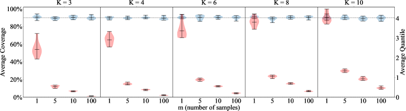
(b) KL

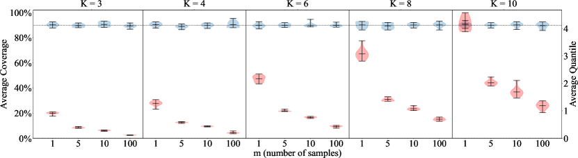
(c) WS

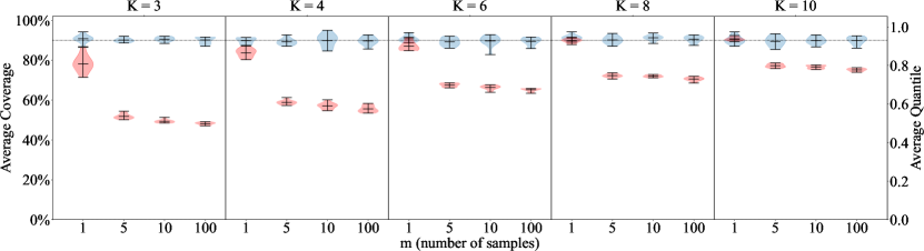
(d) Inner

Figure 6: Coverage and quantile results for synthetic data, where the ground truth distributions are approximated by observing $m$ samples from them. The horizontal dashed lines indicate the nominal coverage levels $1-\alpha=0.9$.

$m$	TV	KL	WS	Inner	SO
1
	$1.00$	$1.00$	$0.70$	$1.00$	$1.00$
5
	$0.46$	$0.67$	$0.39$	$0.22$	$1.00$
10
	$0.64$	$0.58$	$0.68$	$0.00$	$0.74$
100
	$0.06$	$0.09$	$0.09$	$0.00$	$0.43$

Figure 7: Credal sets derived for a synthetic data instance using various credal set predictors. Rows correspond to the number of samples utilized for distribution estimation. The ground truth distribution is marked by an orange square, and its noisy versions are denoted by red squares. In cases employing a first-order learner (first four columns), model predictions are denoted by black circles. The predicted second-order distributions are illustrated via contour plots in the last column, where a second-order learner is employed. The miscoverage rate is $\alpha=0.05$, and the efficiency of each credal set is indicated below it.

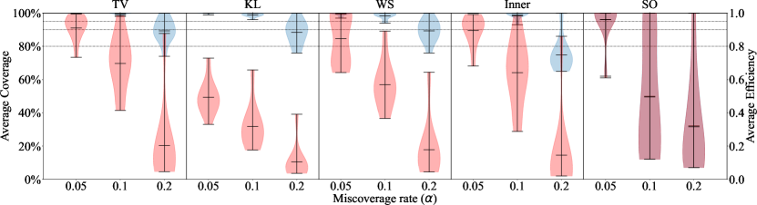
(a) $m=1$.

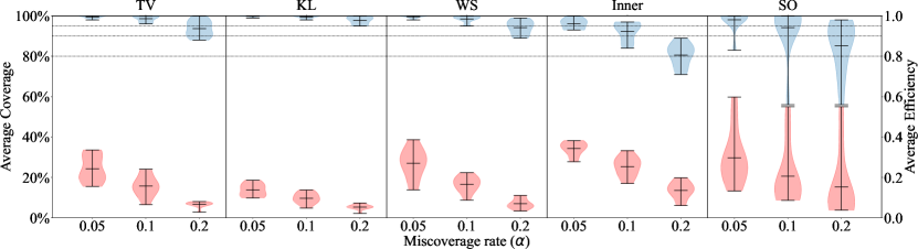
(b) $m=5$.

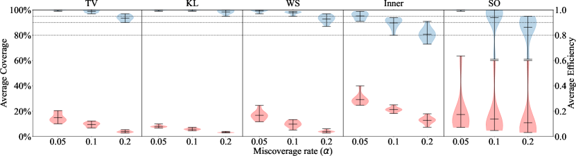
(c) $m=10$.

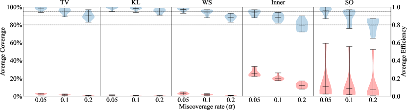
(d) $m=100$.

Figure 8: Coverage and efficiency results of different nonconformity functions applied on the synthetic data with $K=3$. The horizontal dashed lines indicate the nominal coverage levels.

References

- Abellán and Moral [2003] Joaquín Abellán and Serafín Moral. Building classification trees using the total uncertainty criterion. International Journal of Intelligent Systems, 2003.
- Abercrombie et al. [2023] Gavin Abercrombie, Verena Rieser, and Dirk Hovy. Consistency is key: Disentangling label variation in natural language processing with intra-annotator agreement. arXiv preprint arXiv:2301.10684, 2023.
- Angelopoulos et al. [2020] Anastasios Angelopoulos, Stephen Bates, Jitendra Malik, and Michael I Jordan. Uncertainty sets for image classifiers using conformal prediction. arXiv preprint arXiv:2009.14193, 2020.
- Aroyo and Welty [2014] Lora Aroyo and Chris Welty. The three sides of crowdtruth. Human Computation, 1, 2014.
- Aroyo and Welty [2015] Lora Aroyo and Chris Welty. Truth is a lie: Crowd truth and the seven myths of human annotation. AI Magazine, 36, 2015.
- Barber et al. [2021] Rina Foygel Barber, Emmanuel J Candès, Aaditya Ramdas, and Ryan J Tibshirani. Predictive inference with the jackknife+. The Annals of Statistics, 49, 2021.
- Bengs et al. [2022] Viktor Bengs, Eyke Hüllermeier, and Willem Waegeman. Pitfalls of epistemic uncertainty quantification through loss minimisation. In Advances in Neural Information Processing Systems, volume 35, 2022.
- Bengs et al. [2023] Viktor Bengs, Eyke Hüllermeier, and Willem Waegeman. On second-order scoring rules for epistemic uncertainty quantification. In Proceedings of the 40th International Conference on Machine Learning, 2023.
- Bhagavatula et al. [2019] Chandra Bhagavatula, Ronan Le Bras, Chaitanya Malaviya, Keisuke Sakaguchi, Ari Holtzman, Hannah Rashkin, Doug Downey, Wen-tau Yih, and Yejin Choi. Abductive commonsense reasoning. In International Conference on Learning Representations, 2019.
- Bowman et al. [2015] Samuel R. Bowman, Gabor Angeli, Christopher Potts, and Christopher D. Manning. A large annotated corpus for learning natural language inference. In Proceedings of the 2015 Conference on Empirical Methods in Natural Language Processing. Association for Computational Linguistics, 2015.
- Corani and Zaffalon [2008] Giorgio Corani and Marco Zaffalon. Learning reliable classifiers from small or incomplete data sets: The naive credal classifier 2. Journal of Machine Learning Research, 2008.
- Corani et al. [2012] Giorgio Corani, Alessandro Antonucci, and Marco Zaffalon. Bayesian networks with imprecise probabilities: Theory and application to classification. Data Mining: Foundations and Intelligent Paradigms: Volume 1: Clustering, Association and Classification, 2012.
- Depeweg et al. [2018] Stefan Depeweg, Jose-Miguel Hernandez-Lobato, Finale Doshi-Velez, and Steffen Udluft. Decomposition of uncertainty in bayesian deep learning for efficient and risk-sensitive learning. In International Conference on Machine Learning. PMLR, 2018.
- Dietterich and Hostetler [2022] Thomas G Dietterich and Jesse Hostetler. Conformal prediction intervals for markov decision process trajectories. arXiv preprint arXiv:2206.04860, 2022.
- Dumitrache et al. [2019] Anca Dumitrache, FD Mediagroep, Lora Aroyo, and Chris Welty. A crowdsourced frame disambiguation corpus with ambiguity. In Proceedings of NAACL-HLT, 2019.
- Fisch et al. [2022] Adam Fisch, Tal Schuster, Tommi Jaakkola, and Regina Barzilay. Conformal prediction sets with limited false positives. In International Conference on Machine Learning. PMLR, 2022.
- Hora [1996] Stephen C Hora. Aleatory and epistemic uncertainty in probability elicitation with an example from hazardous waste management. Reliability Engineering & System Safety, 54, 1996.
- Hüllermeier and Waegeman [2021] Eyke Hüllermeier and Willem Waegeman. Aleatoric and epistemic uncertainty in machine learning: An introduction to concepts and methods. Machine Learning, 110, 2021.
- Hüllermeier et al. [2022] Eyke Hüllermeier, Sébastien Destercke, and Mohammad Hossein Shaker. Quantification of credal uncertainty in machine learning: A critical analysis and empirical comparison. In Uncertainty in Artificial Intelligence. PMLR, 2022.
- Javanmardi et al. [2023] Alireza Javanmardi, Yusuf Sale, Paul Hofman, and Eyke Hüllermeier. Conformal prediction with partially labeled data. In Conformal and Probabilistic Prediction with Applications. PMLR, 2023.
- Kendall and Gal [2017] Alex Kendall and Yarin Gal. What uncertainties do we need in bayesian deep learning for computer vision? Advances in neural information processing systems, 30, 2017.
- Klir and Wierman [1999] George Klir and Mark Wierman. Uncertainty-based information: elements of generalized information theory, volume 15. Springer Science & Business Media, 1999.
- Kovashka et al. [2016] Adriana Kovashka, Olga Russakovsky, Li Fei-Fei, Kristen Grauman, et al. Crowdsourcing in computer vision. Foundations and Trends® in computer graphics and Vision, 10, 2016.
- Linusson et al. [2020] Henrik Linusson, Ulf Johansson, and Henrik Boström. Efficient conformal predictor ensembles. Neurocomputing, 397, 2020.
- Nie et al. [2020] Yixin Nie, Xiang Zhou, and Mohit Bansal. What can we learn from collective human opinions on natural language inference data? In Proceedings of the 2020 Conference on Empirical Methods in Natural Language Processing (EMNLP). Association for Computational Linguistics, 2020.
- Papadopoulos et al. [2002] Harris Papadopoulos, Kostas Proedrou, Volodya Vovk, and Alex Gammerman. Inductive confidence machines for regression. In Machine Learning: ECML 2002: 13th European Conference on Machine Learning. Springer, 2002.
- Pavlick and Kwiatkowski [2019] Ellie Pavlick and Tom Kwiatkowski. Inherent disagreements in human textual inferences. Transactions of the Association for Computational Linguistics, 7, 2019.
- Reidsma and op den Akker [2008] Dennis Reidsma and Rieks op den Akker. Exploiting ‘subjective’annotations. In Coling 2008: Proceedings of the workshop on Human Judgements in Computational Linguistics, pages 8–16, 2008.
- Romano et al. [2019] Yaniv Romano, Evan Patterson, and Emmanuel Candes. Conformalized quantile regression. Advances in neural information processing systems, 32, 2019.
- Romano et al. [2020] Yaniv Romano, Matteo Sesia, and Emmanuel Candes. Classification with valid and adaptive coverage. Advances in Neural Information Processing Systems, 2020.
- Röttger et al. [2022] Paul Röttger, Bertie Vidgen, Dirk Hovy, and Janet Pierrehumbert. Two contrasting data annotation paradigms for subjective nlp tasks. In Proceedings of the 2022 Conference of the North American Chapter of the Association for Computational Linguistics: Human Language Technologies, 2022.
- Sadinle et al. [2019] Mauricio Sadinle, Jing Lei, and Larry Wasserman. Least ambiguous set-valued classifiers with bounded error levels. Journal of the American Statistical Association, 2019.
- Sale et al. [2023] Yusuf Sale, Michele Caprio, and Eyke Höllermeier. Is the volume of a credal set a good measure for epistemic uncertainty? In Uncertainty in Artificial Intelligence. PMLR, 2023.
- Schaekermann et al. [2016] Mike Schaekermann, Edith Law, Alex C Williams, and William Callaghan. Resolvable vs. irresolvable ambiguity: A new hybrid framework for dealing with uncertain ground truth. In 1st Workshop on Human-Centered Machine Learning at SIGCHI, volume 2016, 2016.
- Sensoy et al. [2018] Murat Sensoy, Lance Kaplan, and Melih Kandemir. Evidential deep learning to quantify classification uncertainty. Advances in neural information processing systems, 31, 2018.
- Sesia and Romano [2021] Matteo Sesia and Yaniv Romano. Conformal prediction using conditional histograms. Advances in Neural Information Processing Systems, 34, 2021.
- Shaker and Hüllermeier [2020] Mohammad Hossein Shaker and Eyke Hüllermeier. Aleatoric and epistemic uncertainty with random forests. In International Symposium on Intelligent Data Analysis. Springer, 2020.
- Snow et al. [2008] Rion Snow, Brendan O’connor, Dan Jurafsky, and Andrew Y Ng. Cheap and fast–but is it good? evaluating non-expert annotations for natural language tasks. In Proceedings of the 2008 conference on empirical methods in natural language processing, 2008.
- Sorokin and Forsyth [2008] Alexander Sorokin and David Forsyth. Utility data annotation with amazon mechanical turk. In 2008 IEEE computer society conference on computer vision and pattern recognition workshops. IEEE, 2008.
- Steinberger and Leeb [2016] Lukas Steinberger and Hannes Leeb. Leave-one-out prediction intervals in linear regression models with many variables. arXiv preprint arXiv:1602.05801, 2016.
- Stutz et al. [2021] David Stutz, Krishnamurthy Dj Dvijotham, Ali Taylan Cemgil, and Arnaud Doucet. Learning optimal conformal classifiers. In International Conference on Learning Representations, 2021.
- Stutz et al. [2023a] David Stutz, Ali Taylan Cemgil, Abhijit Guha Roy, Tatiana Matejovicova, Melih Barsbey, Patricia Strachan, Mike Schaekermann, Jan Freyberg, Rajeev Rikhye, Beverly Freeman, et al. Evaluating ai systems under uncertain ground truth: a case study in dermatology. arXiv preprint arXiv:2307.02191, 2023a.
- Stutz et al. [2023b] David Stutz, Abhijit Guha Roy, Tatiana Matejovicova, Patricia Strachan, Ali Taylan Cemgil, and Arnaud Doucet. Conformal prediction under ambiguous ground truth. Transactions on Machine Learning Research, 2023b.
- Uma et al. [2022] Alexandra Uma, Dina Almanea, and Massimo Poesio. Scaling and disagreements: Bias, noise, and ambiguity. Frontiers in Artificial Intelligence, 2022.
- Uma et al. [2021] Alexandra N Uma, Tommaso Fornaciari, Dirk Hovy, Silviu Paun, Barbara Plank, and Massimo Poesio. Learning from disagreement: A survey. Journal of Artificial Intelligence Research, 72, 2021.
- Vovk [2015] Vladimir Vovk. Cross-conformal predictors. Annals of Mathematics and Artificial Intelligence, 74, 2015.
- Vovk et al. [2017] Vladimir Vovk, Ilia Nouretdinov, Valentina Fedorova, Ivan Petej, and Alex Gammerman. Criteria of efficiency for set-valued classification. Annals of Mathematics and Artificial Intelligence, 81, 2017.
- Vovk et al. [2022] Vladimir Vovk, Alexander Gammerman, and Glenn Shafer. Algorithmic Learning in a Random World. Springer Nature, 2022.
- Walley [1991] Peter Walley. Statistical reasoning with imprecise probabilities, volume 42. Springer, 1991.
- Walley [1996] Peter Walley. Inferences from multinomial data: learning about a bag of marbles. Journal of the Royal Statistical Society Series B: Statistical Methodology, 1996.
- Williams et al. [2018] Adina Williams, Nikita Nangia, and Samuel Bowman. A broad-coverage challenge corpus for sentence understanding through inference. In Proceedings of the 2018 Conference of the North American Chapter of the Association for Computational Linguistics: Human Language Technologies, Volume 1 (Long Papers). Association for Computational Linguistics, 2018.
- Wolf et al. [2019] Thomas Wolf, Lysandre Debut, Victor Sanh, Julien Chaumond, Clement Delangue, Anthony Moi, Pierric Cistac, Tim Rault, Rémi Louf, Morgan Funtowicz, et al. Huggingface’s transformers: State-of-the-art natural language processing. arXiv preprint arXiv:1910.03771, 2019.
- Zaffalon [2002] Marco Zaffalon. The naive credal classifier. Journal of statistical planning and inference, 2002.