Resonance of Gravitational Axions-like Particles

Abstract

The motion of gravitational axion-like particles (ALP) around a Kerr black hole is analyzed, paying attention to resonance and distribution of spectral radiation. We first discuss the computation of $\sqrt{g}{\tilde{R}}_{\mu\nu\rho\rho\sigma}R^{\mu\nu\rho\sigma}$ and its implications with Pontryagin’s theorem and a detailed analysis of Teukolsky’s master equation is done. After carefully analyzing the Teukolsky master equation, we show that this system exhibits resonance when $\omega\gtrsim\mu$ where $\mu$ is the mass of the ALP. A skew-normal distribution can approximate the energy distribution, and we can calculate the mean lifetime of the resonance for black holes with masses between 100 to 1000 $M\textsubscript{$\odot$}$. This range corresponds to a duration between $10^{-1}$s and $10^{41}$s, the observation range used in LIGO data.

I Introduction

Dark matter permeates much of the current cosmology and particle physics research because it can help solve many long-standing problems. However, the search for dark matter encounters difficulties along the way, and so far, one of the most plausible candidates is of very light particles called axions.

Axions are pseudoscalars that were proposed in peccei ; weinberg ; wilczek to solve the strong CP problem and have become the cornerstone of modern particle physics and cosmology.

The axion is described by

$${\cal L}\subset\frac{1}{2}(\partial\varphi)^{2}-\frac{1}{2}m^{2}\varphi^{2}+g\varphi{\tilde{F}}_{\mu\nu}F^{\mu\nu}+\cdots,$$ (1)

where ${\tilde{F}}_{\mu\nu}F^{\mu\nu}$ is the Pontryaguin density for electromagnetic field, $F_{\mu\nu}=\partial_{\mu}A_{\nu}-\partial_{\nu}A_{\mu}$ and $g$ is a coupling constant with dimension $-1$.

The nature of the interaction $\varphi{\tilde{F}}_{\mu\nu}F^{\mu\nu}$ implies that $\varphi$ is a pseudoscalar and the solutions of the equation (plus Maxwell equations)

$$(\Box^{2}+m^{2})\varphi=g\varphi{\tilde{F}}_{\mu\nu}F^{\mu\nu},$$ (2)

provide the ingredients for axion detection arguments sikivie .

In this research, we would like to focus on a different coupling; namely, let us consider the replacement

$$F^{\mu\nu}{\tilde{F}}_{\mu\nu}\to R^{\mu\nu\rho\sigma}{\tilde{R}}_{\mu\nu\rho\sigma},$$ (3)

where $R^{\mu\nu\rho\sigma}{\tilde{R}}_{\mu\nu\rho\sigma}$ is the Pontryaguin-Riemann density, which is

$$R^{\mu\nu\rho\sigma}{\tilde{R}}_{\mu\nu\rho\sigma}=\epsilon^{\rho\sigma\alpha\beta}R_{\mu\nu\rho\sigma}R^{\mu\nu}_{\alpha\beta}.$$ (4)

This kind of system will obey the following system of equations

$$\left(\Box^{2}+m^{2}\right)\varphi = {\bar{g}}R^{\mu\nu\rho\sigma}{\tilde{R}}_{\mu\nu\rho\sigma},$$ (5)

$$G^{\mu\nu}+C^{\mu\nu} = T^{\mu\nu},$$ (6)

where $\Box^{2}=\frac{1}{\sqrt{-g}}\partial_{\mu}(g^{\mu\nu}\partial_{\nu})$ is the Laplace-Beltrami operator, ${\bar{g}}$ is a coupling constant and $C^{\mu\nu}$ is defined as jackiw (Cotton’s tensor)

$$C^{\mu\nu}=\nabla_{\alpha}\varphi\,\epsilon^{\mu\beta\gamma(\mu}\nabla_{\gamma}R^{\nu)}_{\beta}+\left(\nabla_{\sigma}\nabla_{\lambda}\right)\varphi{\tilde{R}}^{\lambda(\mu\nu)\sigma},$$ (7)

with $T_{\mu\nu}$ the energy-momentum tensor for the (pseudo)scalar field in a curved background.

At first sight, the system above retains many properties of the conventional axion but also differs substantially because when coupled to gravity, it becomes dynamically a very different system, These gravitational axions will be denoted generically as ALP. Additionally, the coupling (3) is physically well-motivated witten by the gravitational anomaly and, in analogy with the chiral anomaly where $\pi_{0}\to 2\gamma$ adler ; jack1 , we might also expect the decay $\varphi\to 2g$, where $g$ are gravitons.

In this paper, we will study the problem of ALP in a Kerr black-hole background, and we will focus mainly on resonance and radiation. There are two reasons to consider carefully the phenomenon of resonance; the first is because our research is probably the first example in which Teukolsky’s master equation can be explicitly worked out order by order, and resonance could be a manifest phenomenon; the second reason is that the careful analysis of the resonance allows not only to extract information about the properties of the ALPs but also –if the resonance occurs– it can be seen directly from the spectral radiation curves.

It’s important to note that while Detweiler also examined Kerr’s black holes in a different context in detweiler , his findings are not relevant to our current discussion due to various technical reasons that are unique to the Pontryaguin source we are utilizing.

The paper is structured as follows: in section II, we will begin by studying scalar perturbations and focus on the technical details of the problem. Section III will consider scalar perturbations and their implications with ALP. We will also explain the separation of variables of the Teukolsky equation. Section IV will explain the radial equation with a source in detail and solve it asymptotically. In section V, we will study the emission of gravitational radiation by axion-like particles and numerically calculate the spectral distribution of radiation. Finally, in section VI, we will give our discussions and conclusions. The $S_{\ell}(x)$ properties and essential formulas are in an appendix.

II Axions as scalar perturbations

In this section, we address the problem of solving the equation for axion-like particles in a Kerr background with a Pontryaguin source. The no-source case has been discussed for a long time by Press and Teukolsky press and Damour et al damour , Dolan in dolan , and an updated reference can be found in myung ; yamada .

However, Detweiler in det3 developed a calculation strategy that seems to us to better fit our purpose and that we will use here. Basically, the idea developed in detweiler ; det3 is to consider a Klein-Gordon equation in a Kerr background, and instead of looking for exact solutions, asymptotic solutions can be analyzed to capture the essential physical aspects.

The action is

$$S=\int d^{4}x\sqrt{-g}\left[R+\bar{g}\,R^{\mu\nu\rho\sigma}{\tilde{R}}_{\mu\nu\rho\sigma}+(\partial\varphi)^{2}+\cdots\right].$$ (8)

with $\bar{g}$ the coupling constant. The Kerr metric is assumed, and in Boyer-Lindquist coordinates, it is

$$ds^{2} = -\left(1-\frac{2Mr}{\rho^{2}}\right)dt^{2}-\frac{4Ma\,r}{\rho^{2}}\sin^{2}\theta d\phi dt$$ (9)

$$+ \left(r^{2}+a^{2}+\frac{2Mra^{2}\sin^{2}\theta}{\rho^{2}}\right)\sin^{2}\theta\,d\phi^{2}+\frac{\rho^{2}}{\Delta}dr^{2}+\rho^{2}\,d\theta^{2},$$

where

$$\rho^{2} = r^{2}+a^{2}\cos^{2}\theta,$$

$$\Delta = r^{2}-2Mr+a^{2},$$ (10)

and $a=\frac{J}{M}$ relates the angular momentum with the mass of the black hole.

Note that when $a\to 0$, the angular momentum vanishes, and the metric (10) reduces to the Schwarschild one. The singularities appear when $\Delta=0$, and we have the event horizons

$$r_{\pm}=M\pm\sqrt{M^{2}-a^{2}},$$ (11)

which correspond to the inner and outer event horizons.

The relation $\rho=0$ implies that for $r\to 0$ and $\theta\to\frac{\pi}{2}$, the metric component $g_{tt}\to\infty$. is the true singularity of the Kerr metric. Indeed, the Kretschmann scalar $K=R_{\alpha\beta\gamma\mu}R^{\alpha\beta\gamma\mu}$ for $r\to 0$ is $K_{r\to 0}\propto M^{2}\,\sec^{6}\theta$, showing that $\theta\to\pi/2$ (together with $r\to 0$) is a singularity independent of coordinates.

The calculation of the source term for the scalar field given the action (8), in the Kerr background, yields yunes

$$\sqrt{-g}R^{\mu\rho\sigma}{\tilde{R}}_{\mu\nu\rho\sigma}=-96M^{2}a\,\frac{r\cos\theta\sin\theta}{(r^{2}+a^{2}\cos^{2}\theta)^{5}}(3r^{2}-a^{2}\cos^{2}\theta)(r^{2}-3a^{2}\cos^{2}\theta).$$ (12)

II.1 Pontryagin theorem and subtleties

Equation (12), although correct, cannot be complete because, otherwise, the topological properties of a Kerr black hole would have no physical effect. Several reasons indicate that this is not the case and vorticity is an example that indicates that a turbulent stage of a Kerr black hole must be important in the final dynamics.

Although we will not address the turbulence problem, we would like to point out that the analog of quantized circulation is

$$\int d^{4}x~{}\sqrt{-g}~{}R^{\mu\rho\sigma}{\tilde{R}}_{\mu\nu\rho\sigma}=n,$$ (13)

where $n=0,\pm 1,\pm 2,\cdots$ and (13) is a standard theorem in geometry eguchi .

In our case, the direct calculation yields

$$\int d^{3}x~{}\sqrt{-g}~{}R^{\mu\rho\sigma}{\tilde{R}}_{\mu\nu\rho\sigma}=0,$$ (14)

since due to (12) the Pontryagin density depends only on $r$ and $\theta$.

The first feeling is that a static metric (stationary in this case) does not induce topological properties and, therefore (14) vanishes and the winding number $n=0$.

However, if $n\neq 0$, the integral (14) is not well defined for a stationary metric, and we should regularize it using some reasonableness criterion. Which criterion?, We think it is enough that Pontryagin’s theorem is satisfied.

Thus, we propose the following modification for the Kerr metric

$$\sqrt{-g}~{}R^{\mu\rho\sigma}{\tilde{R}}_{\mu\nu\rho\sigma}\to\sqrt{-g}~{}R^{\mu\rho\sigma}{\tilde{R}}_{\mu\nu\rho\sigma}\delta(x_{0}),$$ (15)

which is consistent with (13).

The above result has a very interesting physical implication because the factor $\delta(t)$ correctly defines the integral on the four-manifold and induces an initial condition to produce gravitational radiation.

Two technical aspects are responsible for these consequences, namely. i) since the source depends on $r$ and $\theta$, the angular momentum along $\varphi$ is conserved, and the general solution of the Teukolsky master equation is a function of $r,\theta$ and $t$; ii) since the LHS is time-dependent, the presence of the $\delta$-function in the RHS becomes mandatory.

III Scalar Perturbations

After discussing these mathematical issues, scalar perturbations for a Kerr black hole can all be written in terms of the Teukolsky master equation teukolsky , which, for the scalar case, reads

$$\frac{\partial}{\partial r}\left(\Delta\frac{\partial\Phi}{\partial r}\right)-\frac{a^{2}}{\Delta}\frac{\partial^{2}\Phi}{\partial\varphi^{2}}-\frac{4Mra}{\Delta}\frac{\partial^{2}\Phi}{\partial\varphi\partial t}-\left(\frac{(r^{2}+a^{2})^{2}}{\Delta}-a^{2}\sin^{2}\theta\right)\frac{\partial^{2}\Phi}{\partial t^{2}}$$

$$+\frac{1}{\sin\theta}\frac{\partial}{\partial\theta}\left(\sin\theta\frac{\partial\Phi}{\partial\theta}\right)+\frac{1}{\sin^{2}\theta}\frac{\partial^{2}\Phi}{\partial\varphi^{2}}-\mu^{2}(r^{2}+a^{2}\cos^{2}\theta)\,\Phi=\kappa\,(r^{2}+a^{2}\cos^{2}\theta)\,{\tilde{R}}_{\mu\nu\rho\sigma}R^{\mu\nu\rho\sigma}\,\delta(t),$$

$$\equiv{T}(x)$$ (16)

with $\kappa$ a constant with canonical dimension $-2$ so that LHS and RHS of the previous equation has dimension ${+1}$.

The source term ${T}(x)$ turns out to be

$$T(x) = 96\kappa M^{2}\,a\frac{r\cos\theta}{(r^{2}+a^{2}\cos^{2}\theta)^{5}}(3r^{2}-a^{2}\cos^{2}\theta)(r^{2}-3a^{2}\cos^{2}\theta)\,\delta(t),$$ (17)

$$\equiv {\cal T}(r,\theta)\,\delta(t).$$

Since the source is $\varphi$-independent, we look for solutions $\Phi(t,r,\theta)$ so that equation (16) reads

$$\frac{\partial}{\partial r}\left(\Delta\frac{\partial\Phi}{\partial r}\right)-\left(\frac{(r^{2}+a^{2})^{2}}{\Delta}-a^{2}\sin^{2}\theta\right)\frac{\partial^{2}\Phi}{\partial t^{2}}-\mu^{2}(r^{2}+a^{2}\cos^{2}\theta)\Phi$$

$$+\frac{1}{\sin\theta}\frac{\partial}{\partial\theta}\left(\sin\theta\frac{\partial\Phi}{\partial\theta}\right) = {\cal T}(r,\theta)\,\delta(t).$$

Then, we look for solutions with the form

$$\Phi(t,r,\theta)=\frac{1}{2\pi}\sum_{\ell}\int e^{\imath{{\omega}}t}R_{\ell}(r)S_{\ell}(c,\theta)\,d\omega,$$ (18)

where the angular function $S_{\ell}(c,\theta)$ satisfies the equation abra ; mike ; lammer2014spheroidal

$$\frac{1}{\sin\theta}\frac{d}{d\theta}\left[\sin\theta\frac{S_{\ell}}{d\theta}\right]+\left(\lambda_{\ell}+c^{2}\cos^{2}\theta\right)S_{\ell}=0,$$ (19)

with $c^{2}=a^{2}(\omega^{2}-\mu^{2})$, and $\lambda_{\ell}$ is the separation constant, which must be determined (see Appendix A for details).

The radial equation reads

$$\frac{d}{dr}\left(\Delta\frac{dR_{\ell}}{dr}\right)+\left[\frac{\omega^{2}(r^{2}+a^{2})^{2}}{\Delta}-(\mu^{2}r^{2}+\omega^{2}a^{2}+\lambda_{\ell})\right]R_{\ell}=A_{\ell}(r),$$ (20)

with $A_{\ell}$ defined through

$$A_{\ell}(r)=\int\,{\cal T}(r,\theta)\,S^{*}_{\ell}(c,\theta)\,d(\cos\theta),$$ (21)

that is, the coefficients of the source, $\cal T$, spanned in the base $S_{\ell}$.

Explicitly,

$$A_{\ell}(r)=96\,\kappa\,M^{2}\,a\,\,r\,\int_{-1}^{1}\frac{x(r^{2}-3a^{2}\,x^{2})}{(r^{2}+a^{2}\,x^{2})^{5}}(3r^{2}-a^{2}\,x^{2})\,{S^{*}}_{\ell}(c,x)dx,$$ (22)

It is hard to find analytical solutions of (20), so let’s do some proper redefinitions. It is convenient to define dimensionless variables.

$$y=\frac{r}{M},\quad\delta=\frac{a}{M},\quad{\bar{\omega}}=\omega\,M,\quad{\bar{\mu}}=\mu\,M,$$

so that the radial equation reads now

$$\frac{d}{dy}\left(\Delta(y)\frac{dR_{\ell}}{dy}\right)+\left[{\bar{\omega}}^{2}\frac{(y^{2}+\delta^{2})^{2}}{\Delta(y)}-({\bar{\mu}}^{2}\,y^{2}+{\bar{\omega}}^{2}\delta^{2}+\lambda_{\ell})\right]R_{\ell}=A_{\ell}(y),$$ (23)

with

$$\Delta(y)=y^{2}-2y+\delta^{2},$$

and

$$A_{\ell}(y)=96\,\frac{\kappa}{M^{2}}\,y\,\delta\,\int_{-1}^{1}\frac{x(y^{2}-3\delta^{2}\,x^{2})}{(y^{2}+\delta^{2}\,x^{2})^{5}}(3y^{2}-\delta^{2}\,x^{2})\,{S^{*}}_{\ell}(c,x)dx.$$

Note that

$$c^{2}=a^{2}(\omega^{2}-\mu^{2})=\delta^{2}({\bar{\omega}}^{2}-{\bar{\mu}}^{2}).$$ (24)

Finally, note also that here $M$ has dimensions of energy^-1 and therefore, $A_{\ell}$ has dimensions of energy, the same dimension as $R_{\ell}(y)$. Then we define

$$Y_{\ell}(y)=\frac{M^{2}}{96\kappa}\,R_{\ell}(My),$$ (25)

and then, the fully dimensionless radial equation can be written as

$$\Delta\frac{d}{dy}\left(\Delta\frac{dY_{\ell}}{dy}\right) + \left[{\bar{\omega}}^{2}(y^{2}+\delta^{2})^{2}-\Delta({\bar{\mu}}^{2}\,y^{2}+{\bar{\omega}}^{2}\delta^{2}+\lambda_{\ell})\right]Y_{\ell}$$ (26)

$$= \frac{M^{2}}{96\kappa}\Delta\,A_{\ell}$$

$$= y\,\delta\,\Delta\,\int_{-1}^{1}\frac{x(y^{2}-3\delta^{2}\,x^{2})}{(y^{2}+\delta^{2}\,x^{2})^{5}}(3y^{2}-\delta^{2}\,x^{2})\,{S^{*}}_{\ell}(c,x)dx.$$

$$\equiv \tilde{A}_{\ell}(y).$$

The following sections are devoted to the study of numerical solutions to this equation, and also to the analysis of asymptotic structure.

IV Radial Equation: Asymptotic analysis

In this section, we will make an asymptotic analysis of the radial equation, which, as we show below, has important physical consequences in the Teukolsky master equation for pseudoscalar fields.

In effect, Pontryagin’s term is a very special source because being in the case that we consider a function of the form $F(r,\theta)$, it implies that for even values of $\ell$ the source vanishes while for odd values, this is not the case.

To analyze the asymptotic regions, we first change coordinates to tortoise coordinates $y_{*}$ defined through

$$\frac{dy_{*}}{dy}=\frac{y^{2}+\delta^{2}}{\Delta(y)}=\frac{y^{2}+\delta^{2}}{y^{2}-2y+\delta^{2}}.$$ (27)

Equation (26) reads

$$(y^{2}+\delta^{2})\frac{d}{dy_{*}}\left((y^{2}+\delta^{2})\frac{dY_{\ell}}{dy_{*}}\right)+\left[{\bar{\omega}}^{2}(y^{2}+\delta^{2})^{2}-\Delta({\bar{\mu}}^{2}\,y^{2}+{\bar{\omega}}^{2}\delta^{2}+\lambda_{\ell})\right]Y_{\ell}=\tilde{A}_{\ell}(y),$$ (28)

where all functions of $y$ are understood as functions of $y_{*}$ trough $y=y(y_{*})$, while $Y_{\ell}(y_{*})\equiv R(y(y_{*}))$. By defining the function $W(y_{*})$ through

$$Y_{\ell}(y_{*})=(y^{2}+\delta^{2})^{-1/2}\,W_{\ell}(y_{*}),$$

equation (28) is

$$\frac{d^{2}\,W_{\ell}}{dy_{*}^{2}}+\left[{\bar{\omega}}^{2}-\frac{\Delta}{(y^{2}+\delta^{2})^{2}}\left({\bar{\mu}}^{2}\,y^{2}+{\bar{\omega}}^{2}\delta^{2}+\lambda_{\ell}+\frac{1}{(y^{2}+\delta^{2})^{2}}\left(\Delta\,\delta^{2}+2y(y^{2}-\delta^{2})\right)\right)\right]\,W_{\ell}=\bar{A}_{\ell}(y_{*}),$$ (29)

with

$$\bar{A}_{\ell}(y_{*})=\frac{\tilde{A}_{\ell}(y)}{(y^{2}+\delta^{2})^{3/2}}.$$ (30)

That is, $W_{\ell}$ satisfies the Schrödinger-type equation

$$\frac{d^{2}\,W_{\ell}}{dy_{*}^{2}}+{V_{\mbox{\tiny{eff}}}}(y_{*})\,W_{\ell}=\bar{A}_{\ell}(y_{*}).$$ (31)

We are interested in the solutions of (31) in the asymptotic regions $y_{*}\to\infty$ (solution at infinity) and $y_{*}\to-\infty$ (the near horizon solution).

We first study the behavior of the source in these limits.

IV.1 The source

Since $S_{\ell}$ is a superposition of Legendre’s polynomial $P_{\ell}(x)$ (see Appendix A), the source in (26) is

$$\tilde{A}_{\ell} = y\,\Delta\,\delta\,\int_{-1}^{1}\frac{x(y^{2}-3\delta^{2}\,x^{2})}{(y^{2}+\delta^{2}\,x^{2})^{5}}(3y^{2}-\delta^{2}\,x^{2})\,{S^{*}}_{\ell}(c,x)dx,$$

$$= y\,\Delta\,\delta\,\sum_{\ell^{\prime}}B_{\ell,\ell^{\prime}}(c)\int_{-1}^{1}\frac{x(y^{2}-3\delta^{2}\,x^{2})}{(y^{2}+\delta^{2}\,x^{2})^{5}}(3y^{2}-\delta^{2}\,x^{2})\,P_{\ell}^{\prime}(x)dx,$$

$$= y\,\Delta\,\delta\,\sum_{\ell^{\prime}=0}B_{\ell,2\ell^{\prime}+1}(c)\int_{-1}^{1}\frac{x(y^{2}-3\delta^{2}\,x^{2})}{(y^{2}+\delta^{2}\,x^{2})^{5}}(3y^{2}-\delta^{2}\,x^{2})\,P_{2\ell^{\prime}+1}(x)dx,$$

$$= \sum_{\ell^{\prime}=0}B_{\ell,2\ell^{\prime}+1}(c)\,{\cal I}_{2\ell^{\prime}+1}(y,\delta),$$ (33)

with

$${\cal I}_{2\ell^{\prime}+1}(y,\delta)=y\,\Delta\,\delta\,\int_{-1}^{1}\frac{x(y^{2}-3\delta^{2}\,x^{2})}{(y^{2}+\delta^{2}\,x^{2})^{5}}(3y^{2}-\delta^{2}\,x^{2})\,P_{2\ell^{\prime}+1}(x)dx.$$ (34)

It can be shown that coefficients $B$ have the following property

$$B_{2m,2n+1}=0=B_{2n+1,2m},\quad m,n\in\{0,1,2,\cdots\},$$ (35)

and, therefore

$$\bar{A}_{2n}=0,\quad n\in\{0,1,2,\cdots\}$$ (36)

In our numerical analysis, we consider $\ell=0,1,2,3$, then the relevant functions for us are ${\cal I}_{1}$ and ${\cal I}_{3}$, shown in Figure 1 for two different values of $\delta$. The maximal contribution occurs in the region $y_{*}\lesssim 0$, that is, toward the outer horizon, while contributions from $y_{*}\to\infty$ are negligible.

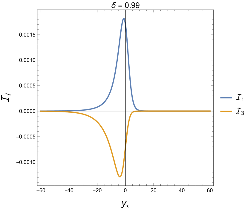
(a) Function ${\cal I}_{\ell}$ vs rescaled tortoise coordinate $y_{*}$ for $\delta=0.99$

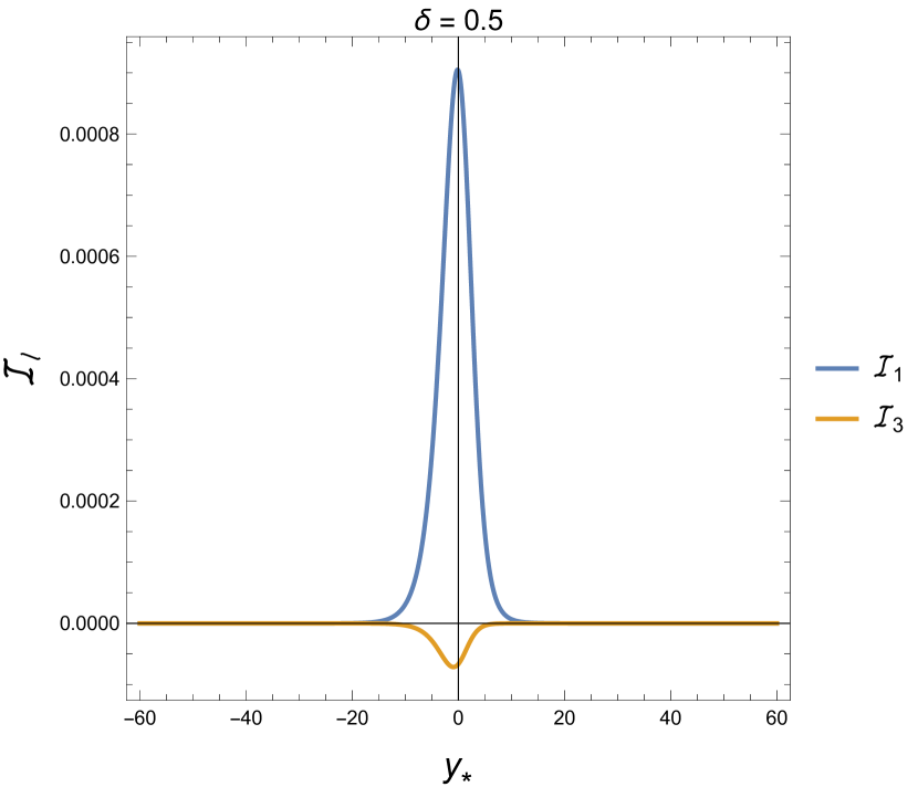
(b) Function ${\cal I}_{\ell}$ vs rescaled tortoise coordinate $y_{*}$ for $\delta=0.5$

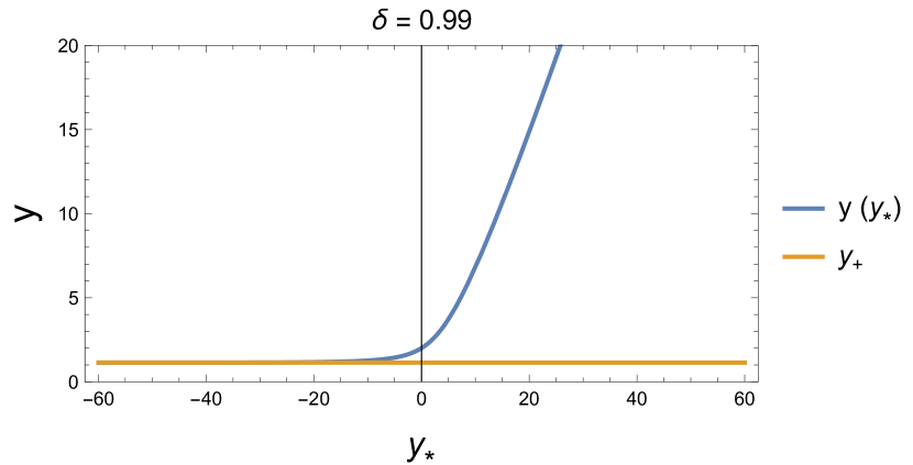
(c) The coordinate $y$ as function of $y_{*}$ and the horizon $y_{+}$.

Figure 1: Panels (a) and (b) show the function ${\cal I}_{\ell}$ defined in (34) for two different black hole’s rotation velocity $\delta=a/M$ for $\ell=1$, and $\ell=3$. Panel (c) shows $y(y_{*})$ and the coincidence of $y_{+}$ (the horizon) with $y_{*}\to-\infty$

In (1(c)) we can check that for $\delta=0.99$, the horizon is reached at $y_{*}\approx 20$. Then, numerically, $|y_{*}|>30$ is a good approximation for the limits $y_{*}\to\pm\infty$.

The source terms in (31) is, therefore, zero for even values of $\ell$, while for the two other cases under analysis, they are

$$\bar{A}_{1}(y_{*}) = (y^{2}+\delta^{2})^{-3/2}(B_{1,1}(c)\,{\cal I}_{1}+B_{1,3}(c)\,{\cal I}_{3}),$$ (37)

$$\bar{A}_{3}(y_{*}) = (y^{2}+\delta^{2})^{-3/2}(B_{3,1}(c)\,{\cal I}_{1}+B_{3,3}(c)\,{\cal I}_{3}),$$ (38)

with $B_{1,1},B_{1,3},B_{3,1},B_{3,3}$ given in Appendix A, and

$${\cal I}_{1} = \frac{2y\delta\Delta(y^{2}-\delta^{2})}{(y^{2}+\delta^{2})^{4}},$$ (39)

$${\cal I}_{3} = \frac{5\Delta}{2\delta^{4}}\tan^{-1}\left(\frac{\delta}{y}\right)-\frac{y\Delta}{6\delta^{3}\left(y^{2}+\delta^{2}\right)^{4}}\left(15y^{6}+55y^{4}\delta^{2}+73y^{2}\delta^{4}+57\delta^{6}\right).$$ (40)

IV.2 Numerical Solutions

The potential ${V_{\mbox{\tiny{eff}}}}$ in the limits previously discussed has the following asymptotic behavior

$${V_{\mbox{\tiny{eff}}}}=\begin{cases}k^{2}+{\cal O}(y^{-1}),&y_{*}\to\infty~{}~{}(y\to\infty),\\ {\bar{\omega}}^{2}+{\cal O}(y-y_{+}),&y_{*}\to-\infty~{}~{}(y\to y_{+}),\end{cases}$$ (41)

with $k^{2}={\bar{\omega}}^{2}-\bar{\mu}^{2}\geq 0$. We can treat the equation as an homogeneous equation in these limits since the source can be taken zero there, as shown in Fig. 1.

The asymptotic solutions are, therefore

$$W^{(+)}(y_{*}) \sim A^{(+)}\,e^{\imath{\bar{\omega}}y_{*}}+C^{(+)}\,e^{-\imath{\bar{\omega}}y_{*}}\quad(y_{*}\to-\infty),$$ (42)

$$W^{(\infty)}(y_{*}) \sim A^{(\infty)}\,e^{\imath ky_{*}}+C^{(\infty)}\,e^{-\imath ky_{*}}\quad(y_{*}\to\infty).$$ (43)

Following (detweiler ), we choose $A^{(+)}=1,C^{(+)}=0$. Numerical solutions for this choice are displayed in Fig (2) for $\ell=0,1$

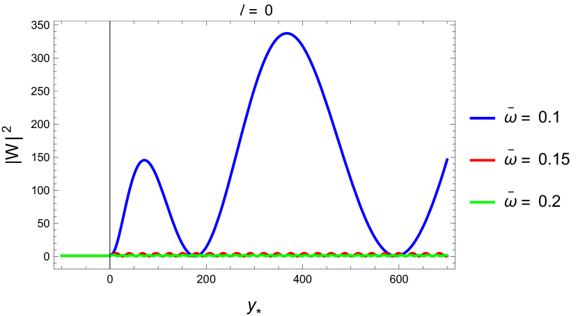
(a) $|W|^{2}$ for ${\bar{\omega}}\sim\bar{\mu}$ and $\ell=0$.

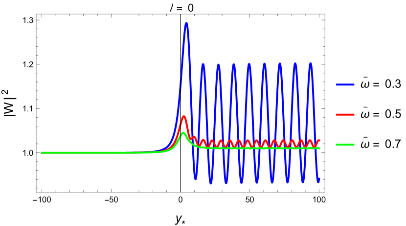
(b) $|W|^{2}$ for ${\bar{\omega}}>\bar{\mu}$ and $\ell=0.$

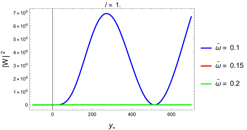
(c) $|W|^{2}$for ${\bar{\omega}}\sim\bar{\mu}$ and $\ell=1$.

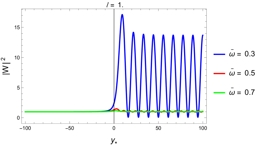
(d) $|W|^{2}$ for ${\bar{\omega}}>\bar{\mu}$ and $\ell=1$.

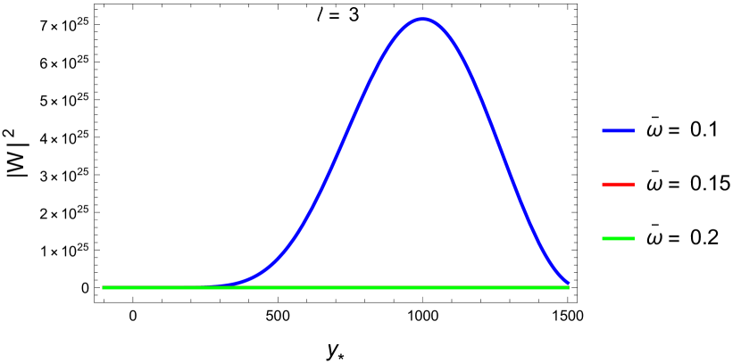
(e) $|W|^{2}$ for ${\bar{\omega}}\sim\bar{\mu}$, and $\ell=3$.

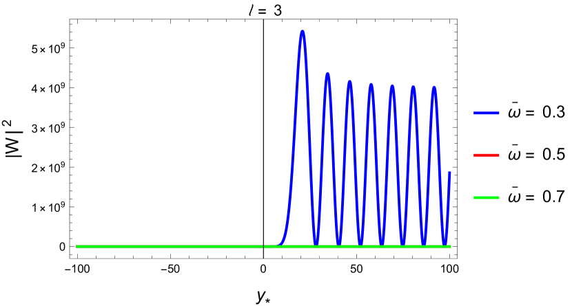
(f) $|W|^{2}$ for ${\bar{\omega}}>\mu$, and $\ell=3$.

Figure 2: The amplitude $|W|^{2}$ for $\delta=0.99$, $\bar{\mu}=0.1$ and $\ell=0,1$ for different values of ${\bar{\omega}}$.

As we pointed out before, the source components $\bar{A}_{\ell}$ are non-zero for $\ell$ odd (shown in Figures 1(a) and 1(b)). It is interesting to compare with the sourceless case.

In Figure 3, we plot the case $\ell=1$ and $\ell=3$ for different values of ${\bar{\omega}}$, comparing the solution with and without source.

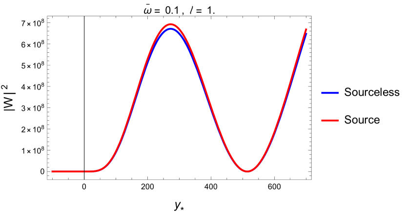
(a) $|W|^{2}$ for ${\bar{\omega}}\sim\bar{\mu}$ and $\ell=1$. Effect of the source term.

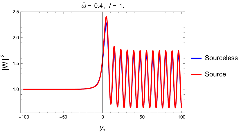
(b) $|W|^{2}$ for ${\bar{\omega}}>\bar{\mu}$ and $\ell=1$. Effect of the source term.

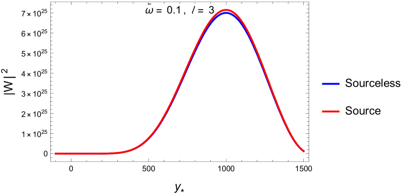
(c) $|W|^{2}$ for ${\bar{\omega}}\sim\bar{\mu}$ and $\ell=3$. Effect of the source term.

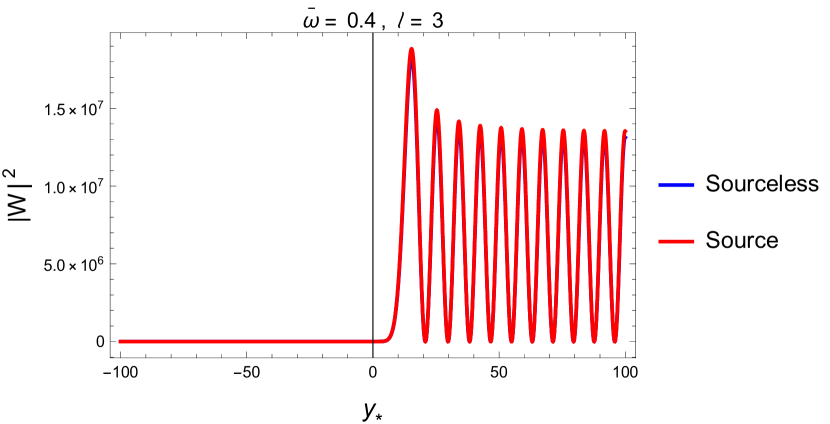
(d) $|W|^{2}$ for ${\bar{\omega}}>\bar{\mu}$ and $\ell=3$. Effect of the source term.

Figure 3: The amplitude $|W|^{2}$ for $\delta=0.99$, $\bar{\mu}=0.1$ and $\ell=1,3$ for the cases with and without source term

The source mainly affects the maxima (peaks) of $|W^{2}|$, but not the position of these peaks. Besides, the amplitude increases for higher values of $\ell$, and the highest amplitudes occur for ${\bar{\omega}}\sim\bar{\mu}$. This last condition, $c\sim 0$, corresponds to the longwave approximation.

Indeed, the equation (22) is analogous to the partial wave method in quantum mechanics theory but spheroidal harmonics instead of Legendre polynomials.

In (24) we can write $c^{2}=a^{2}(\omega^{2}-{\mu}^{2})=a^{2}|{p}|^{2}\sim\left(\frac{a}{\lambda}\right)^{2}$, where $|{p}|$ is the momentum of the scalar field, and therefore the limit $c\to 0$ is equivalent to $a\ll\lambda$, which is the well-known long-wave approximation (LWA) introduced by Isaacson isaacson in gravitational radiation .

In this approximation

$$S_{\ell}(c,x)\approx P_{\ell}(x),$$ (44)

and $\lambda_{\ell}\approx\ell(\ell+1)$.

We can compare the solutions obtained by setting $c=0$ with those coming from the general treatment in the Appendix A. The results are shown in Figure 4.

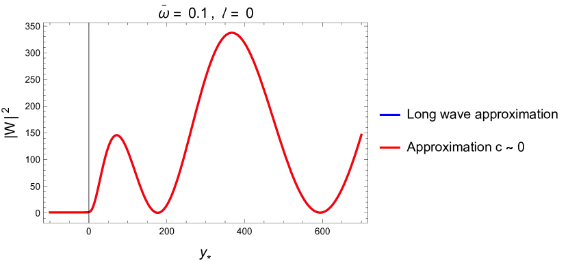
(a) $|W|^{2}$ obtained in the long wave approximation compared with the approximated solution for ${\bar{\omega}}=\bar{\mu}$ and $\ell=0$.

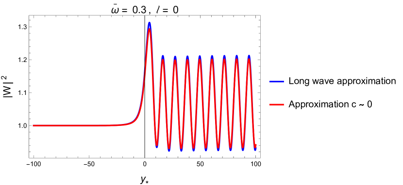
(b) $|W|^{2}$ obtained in the long wave approximation compared with the approximated solution for ${\bar{\omega}}>\bar{\mu}$ and $\ell=0$.

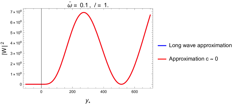
(c) $|W|^{2}$ obtained in the long wave approximation compared with the approximated solution for ${\bar{\omega}}=\bar{\mu}$ and $\ell=1$.

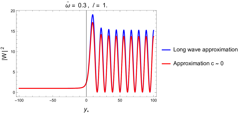
(d) $|W|^{2}$ obtained in the long wave approximation compared with the approximated solution for ${\bar{\omega}}>\mu$ and $\ell=1$.

Figure 4: Compared amplitudes $|W|^{2}$ for $\delta=0.99$, $\bar{\mu}=0.1$ and different $\ell$. In one case, we use the long wave approximation, while the other corresponds to the solution calculated with the perturbative approach described in the Appendix A

The numerical solutions presented in figures 1, 2, 3 and 4 shows that: a) the source considered in the present work is relevant in the region near the horizon, but in the limit $y_{*}\to\pm\infty$, the equation for the scalar field can be safely taken as (31) with the asymptotic form of the effective potential given in (41) and sourceless; b) for numerical purposes, the choice $|y_{*}|\gtrsim 100$ is enough to guarantee we are close enough to the horizon and infinity (depending on the sign of $y_{*}$); c) the case ${{\omega}}\sim\mu$ can be treated using the long wave approximation, or the expressions for $\lambda_{\ell}$ obtained in the Appendix A.

In the following section, we will discuss the radiation pattern of the solutions analyzed here.

V Emission of Radiation

Following detweiler , the emission of axions radiation due to the source (12), per unit frequency interval per solid angle $d\Omega$ is

$$\frac{d^{2}E_{\ell}}{d{\bar{\omega}}d\Omega}=\left(\frac{{S_{\ell}(\theta)}}{\sqrt{2\pi}}\right)^{2}\frac{1}{|2\,A^{(\infty)}(\bar{\omega})|^{2}}\left|\int_{-\infty}^{\infty}W^{(\infty)}(y_{*})\,\bar{A}_{\ell}(y_{*})\,dy_{*}\right|^{2}.$$ (45)

The angular term $S_{\ell}^{2}$ depends on $c^{2}=\omega^{2}-\mu^{2}$ but will omit this in the analysis since it represents a small contribution, as seen in the appendix, where this term is plotted as a function of the frequency.

The term $|A^{(\infty)}(\bar{\omega})|^{-2}\equiv Q(\bar{\omega})$ is obtained from the numerical solution of (31) with initial conditions

$$W(y_{*})=e^{\imath\bar{\omega}y_{*}},\quad W^{\prime}(y_{*})=\imath\bar{\omega}\,e^{\imath\bar{\omega}y_{*}},\quad(y_{*}\to-\infty),$$

and therefore

$$A^{(\infty)}(\bar{\omega})=\lim_{y_{*}\to\infty}\left(\frac{\sqrt{\bar{\omega}^{2}-\bar{\mu}^{2}}\,W(y_{*})-\imath W^{\prime}(y_{*})}{2\sqrt{\bar{\omega}^{2}-\bar{\mu}^{2}}}\right),$$ (46)

Another interesting quantity to characterize the radiation emission is the fractional energy gain from the monochromatic wave sent from infinity. In our case, this quantity is

$$Z=\left|\frac{C^{(\infty)}}{A^{(\infty)}}\right|^{2}-1,$$ (47)

where $C^{(\infty)}$ is calculated in a similar way as $A^{(\infty)}$:

$$C^{(\infty)}(\bar{\omega})=\lim_{y_{*}\to\infty}\left(\frac{\sqrt{\bar{\omega}^{2}-\bar{\mu}^{2}}\,W(y_{*})+\imath W^{\prime}(y_{*})}{2\sqrt{\bar{\omega}^{2}-\bar{\mu}^{2}}}\right),$$ (48)

Figures 5 show $Q$ and $Z$ for $\ell=0$ and $\ell=1$. For the case $\ell=0$ (and for all even values of $\ell$), the source term is zero; however, for even values of $\ell$, the source is relevant. Figures 5(c) and 5(d) show how different the factors $Z$ and $Q$ are when the source is considered.

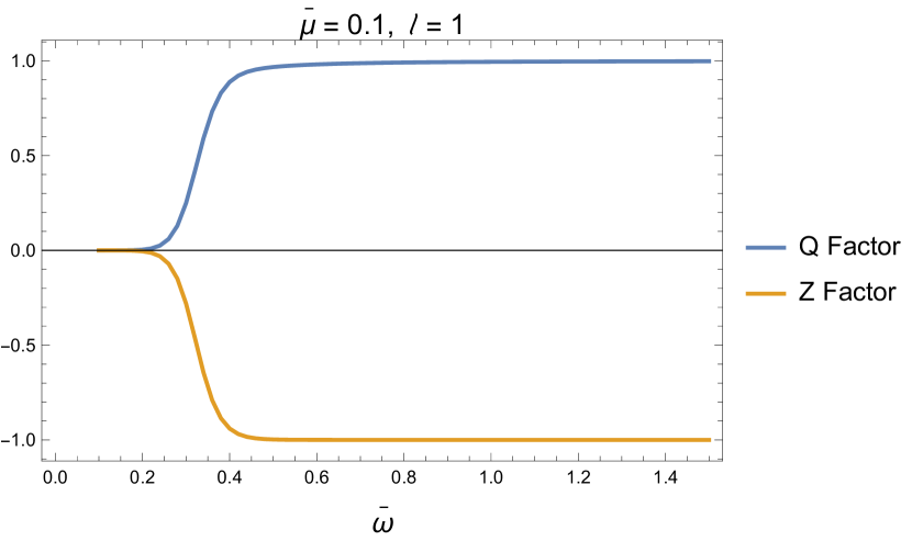
(a) Factors $Q$ and $Z$ for $\bar{\mu}=0.1$ and $\ell=1$.

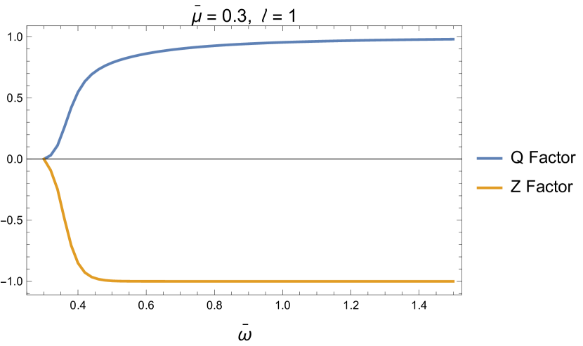
(b) Factors $Q$ and $Z$ for $\bar{\mu}=0.3$ and $\ell=1$

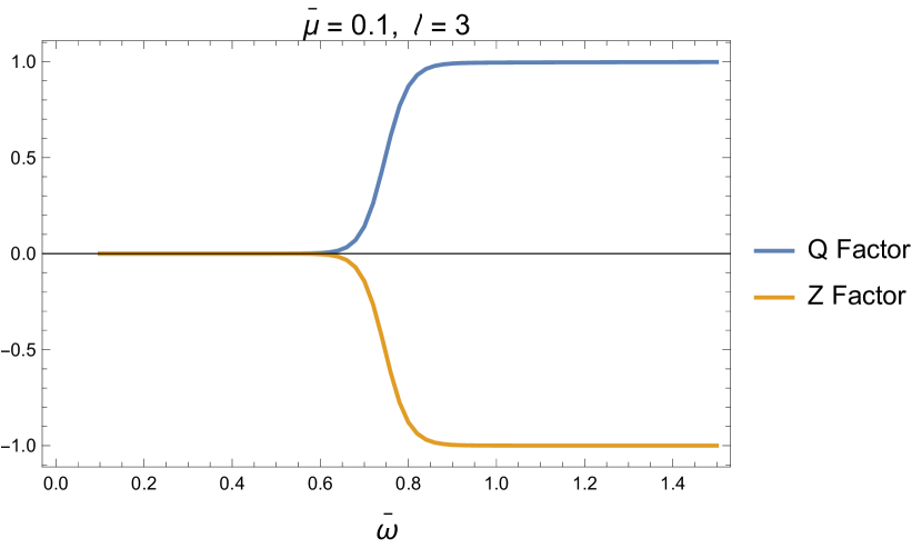
(c) Factors $Q$ and $Z$ for $\bar{\mu}=0.1$ and $\ell=3$

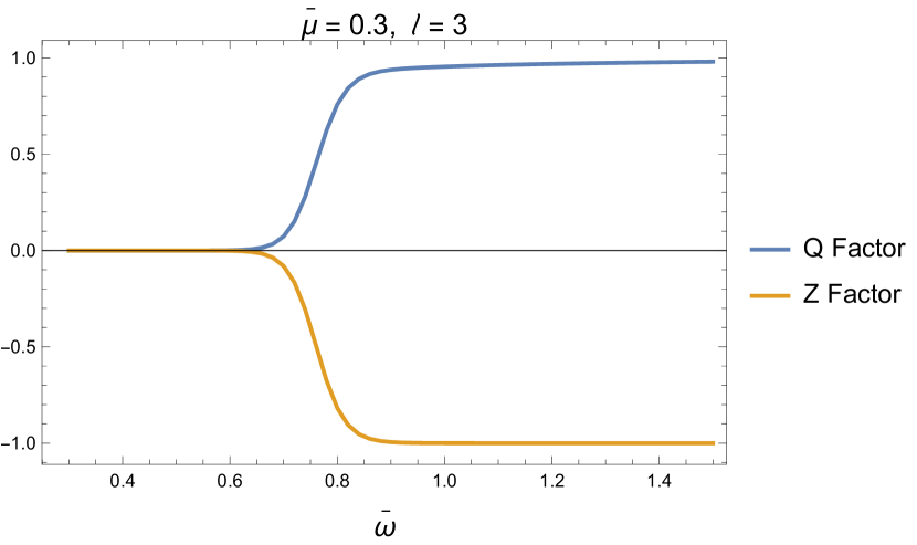
(d) Factors $Q$ and $Z$ for $\bar{\mu}=0.3$ and $\ell=3$.

Figure 5: Factors $Q$ and $Z$ defined in the text for different values of $\ell$ and $\bar{\mu}$. In all panels, $\delta=0.99$.

With these results, we numerically calculate the total energy radiated to infinity up to the constant coming from the solid angle integration, that is

$$\frac{dE}{d{\bar{\omega}}}=\frac{1}{|2\,A^{(\infty)}(\bar{\omega})|^{2}}\left|\int_{-\infty}^{\infty}W^{(\infty)}(y_{*})\,\bar{A}_{\ell}(y_{*})\,dy_{*}\right|^{2},$$ (49)

which is not zero only for odd values of $\ell$. In our case, this is $\ell=1,3$. The results are plotted in Figure 6

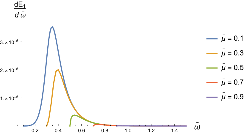
(a) Factors $Q$ and $Z$ for $\ell=0$.

Figure 6: Radiated energy as function of $\bar{\omega}$ for different masses and $\ell=1,\delta=0.99$

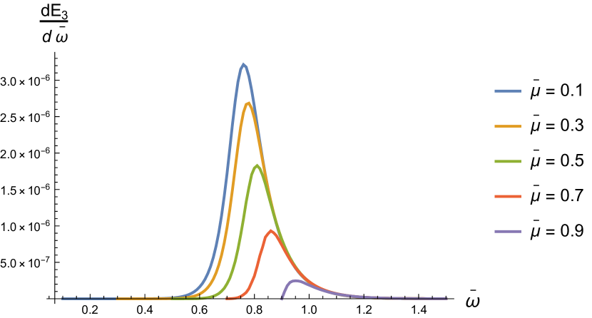
(a) Factors $Q$ and $Z$ for $\ell=0$.

Figure 7: Radiated energy as function of $\bar{\omega}$ for different masses and $\ell=1,\delta=0.99$.

Let us comment on the results shown in this numerical analysis. According to Detweiler in detweiler , a sharp maximum in $Q$ signals a resonant frequency at which a black hole resonance occurs. In our case, this resonance does not happen, as seen in Figure 5.

To understand this, first note that our initial condition (numerical integration condition) is $|W|^{2}=|A^{(+)}|^{2}=1$ near the horizon ($y_{*}\to-\infty$ or, numerically, $y_{*}=-100$). On the other hand, functions $Z$ and $Q$ start from zero at the initial frequency $\bar{\omega}=\bar{\mu}$, then $Z$ increase while $Q$ decrease, which happens during a frequency interval, let’s say $\Delta\bar{\omega}$. By denoting the half of such interval as $\bar{\omega}_{c}$, the function $Z$ behaves as follow

$$Z=\left\{\begin{array}[]{lcl}0&&\bar{\omega}\lessapprox\bar{\omega}_{c}-\Delta\bar{\omega},\\ -1&&\bar{\omega}\gtrapprox\bar{\omega}_{c}+\Delta\bar{\omega},\end{array}\right.$$ (50)

and a similar expression for $Q$, changing the last line to $1$.

From the definition of $Q$ and $Z$, previous behavior is understood due to the following. For $\bar{\omega}\lessapprox\bar{\omega}_{c}-\Delta\bar{\omega}$, the denominator in (46) produces a divergence that is the responsible for $Q\to 0$. Instead, for $Z$, such divergence is not present since $Z$ depends on the ratio $C^{(\infty)}/A^{(\infty)}$ (see the definition of $C^{(\infty)}$ in (48) and then for this frequency range, $|C^{(\infty)}|^{2}\sim|A^{(\infty)}|^{2}$

Instead, for $\bar{\omega}\gtrapprox\bar{\omega}_{c}+\Delta\bar{\omega}$, the condition $|A^{(\infty)}|^{2}\sim 1$ and $|C^{(\infty)}|^{2}\sim 0$ is consistent with the behavior of $Z$ and $Q$ factors.

Since the $Z$ factor is the fractional energy gain of a wave of frequency $k=\sqrt{\bar{\omega}^{2}-\bar{\mu}^{2}}$ sent from the infinity that is scattered from the BH. In the zone where $Z\sim 0$, part of the incoming wave is scattered (indeed, in this frequency range $|C^{(\infty)}|\sim|A^{(\infty)}|$, while in the region in which $Z\to-1$, no scattered wave is present, indicating a complete absorption of the signal.

Therefore, the energy radiated should be centered in the transition zone, the $\Delta\omega$ region. Figures 6 and 7 precisely show this behavior.

VI Conclusions

This research paper explores the movement of gravitational axions in a Kerr black hole background using analytical and numerical methods. One interesting finding is that resonance occurs when $\omega\gtrsim\mu$, similar to the Detweiler-resonance discussed in detweiler . However, the Detweiler-resonance is related to a massless scalar. This research concludes that this resonance always occurs if $\ell$ is odd and a Pontryaguin-like source is present.

Another important observation is that Figures 6 and 7 show that the spectral maxima shifts to the right, and the radiated power decreases with ${\bar{\omega}}$. Additionally, the maximum becomes significantly smaller when $\ell$ grows. However, it is interesting to note qualitatively that the curves can be reasonably approximated as Gaussian for small $\bar{\mu}$.

For $\bar{\mu}\gtrsim 0.3$, the Gaussian starts to be asymmetric with a deviation to the right. We found that the function

$$f(\bar{\omega})=a\,e^{-\frac{(x-\xi)^{2}}{2\,\sigma^{2}}}\left(1+\mbox{\small{erf}}\left(\frac{\alpha\,(x-\xi)}{\sqrt{2}\,\sigma}\right),\right)$$ (51)

is well-fitted to the curves of the radiated power. Here, $\mbox{\small{erf}}(x)$ is the error function

$$\mbox{\small{erf}}(x)=\frac{2}{\sqrt{\pi}}\int_{0}^{x}e^{-t^{2}}\,dt.$$

The function $f$ in (51) is proportional to the probability density of a skew-normal distribution, with proportionality constant $a$ and for this distribution, it is known that the mean value is

$$\mbox{Mean}=\mu+\frac{\sqrt{\frac{2}{\pi}}\alpha\sigma}{\sqrt{1+\alpha^{2}}},$$

and the variance

$$\mbox{Var}=\sigma^{2}\left(1-\frac{2\alpha^{2}}{\pi(1+\alpha^{2})}\right).$$

So, an estimation of the mean width of the curves in Figures 6 and 7 is given by $2\sqrt{\mbox{Var}}$. That is

$$\Delta\bar{\omega}\approx 2\sigma\sqrt{1-\frac{2\alpha^{2}}{\pi(1+\alpha^{2})}}.$$

The following table resumes these results

The mean value and variance for different $\ell$ and $\bar{\mu}$ from Figures 6 and 7

$\ell$	$\bar{\mu}$	$\langle\bar{\omega}\rangle$	$\Delta\bar{\omega}$
1	0.1	0.38	0.16
	0.3	0.44	0.16
	0.5	0.61	0.15
	0.7	0.81	0.15
	0.9	1.01	0.15
3	0.1	0.78	0.15
	0.3	0.80	0.15
	0.5	0.84	0.14
	0.7	0.90	0.14

Estimating the mean lifetime of these resonances as (dimensionful quantities)

$$\tau\approx(\Delta\omega)^{-1}=\frac{M}{\Delta\bar{\omega}}\approx 5\times 10^{38}\left(\frac{M}{M_{\odot}}\right)~{}~{}~{}[{\mbox{s}}]$$

Then, for example, for primordial black holes with the masses ranging from Planck mass ($\sim 10^{-37}M_{\odot}$) to masses of order $10^{3}M_{\odot}$ will cause pulses with a mean lifetime from $10^{-1}$ [s] up to $10^{41}$ [s]$\sim 10^{34}$ years, that is (in the last case) a mean lifetime well beyond the universes’s age.

It’s worth noting that the resonance for gravitational axions discussed in this paper is distinct from the one studied in Detweiler’s work. In Detweiler’s case detweiler , the resonance is observed as a divergence of the factor $Q({\bar{\omega}})$, whereas in our case, $Q({\bar{\omega}})$ approaches 1 as ${\bar{\omega}}$ tends to infinity.

In conclusion, observing very sharp resonances in radiation patterns is possible depending on the black holes’ mass. For instance, if the black holes have masses between 100 and 1000 $M\textsubscript{$\odot$}$, the lifetime of these resonances falls within the range of observability in LIGO soda .

Appendix A The angular equation

In this appendix, we review the solution of (19) following the analysis by S. Teukolsky in (teukolsky ). First, define as usual $x=\cos\theta$, so that the angular equation is now

$$\frac{d}{dx}\left[(1-x^{2})\frac{d{S}}{dx}\right]+(\lambda+c^{2}x^{2}){S}=0.$$ (52)

In reference (teukolsky ), a method for treating the case of any spin $s$ and third component of angular momentum, $m$, is discussed. However, we restrict here to the case of interest for us, that is, $m=0$ and $s=0$, which is just previous equation.

The idea is to treat the $c^{2}x^{2}$ term as a perturbation (not necessarily infinitesimal). The order zero operator is

$$\frac{d}{dx}\left[(1-x^{2})\frac{d{S}}{dx}\right]=-\lambda{S},$$ (53)

with the known (normalized) solution

$${S}_{\ell}(x)=\sqrt{\frac{2\ell+1}{2}}P_{\ell}(x),$$ (54)

with $\lambda=\ell(\ell+1)$ ( $\ell=0,1,2\cdots$), and $P_{\ell}(x)$ the Legendre’s polynomial of degree $\ell$.

The continuation method wasserstrom for calculating eigenfunction and eigenvalues in (52) considers $c$ as a parameter, and then the equation under study is

$$\left[(1-x^{2}){{S}^{\prime}}_{\ell}\right]^{\prime}+(\lambda_{\ell}(c)+c^{2}x^{2}){S}_{\ell}=0,$$ (55)

with ^′ denoting derivatives respect to $x$ and ${S}_{\ell}=S_{\ell}(c,x)$.

By taking the derivative with respect to $c$ in the previous equation (denoted by a dot in what follows), one obtains

$$\left[(1-x^{2})\dot{{S}^{\prime}_{\ell}}\right]^{\prime}+(\dot{\lambda}_{\ell}+2cx^{2}){S}_{\ell}+(\lambda_{\ell}+c^{2}x^{2})\dot{S}_{\ell}=0.$$ (56)

From here, it is possible to find a set of first-order differential equations for $\lambda_{\ell}(c)$ and ${S}_{\ell}$. Indeed, multiplying the last equation by ${S}_{\ell}$ followed by an $x$ integration one gets

$$\int dx{S}_{\ell}\left[(1-x^{2})\dot{{S}^{\prime}_{\ell}}\right]^{\prime}+\int dx{S}_{\ell}(\dot{\lambda}_{\ell}+2cx^{2}){S}_{\ell}+\int dx{S}_{\ell}(\lambda_{\ell}+c^{2}x^{2})\dot{{S}_{\ell}}=0.$$ (57)

The first term can be integrated by parts twice giving (boundary terms cancel)

$$\int dx~{}{S}_{\ell}\left[(1-x^{2})\dot{{S}^{\prime}_{\ell}}\right]^{\prime} = \int dx~{}\dot{{S}}_{\ell}\left[(1-x^{2}){{S}^{\prime}_{\ell}}\right]^{\prime},$$ (58)

$$=- \int dx~{}\dot{{S}}_{\ell}(\lambda_{\ell}+c^{2}x^{2}){S}_{\ell}.$$

Then, the first and second terms cancel in (57). Finally,

$$\dot{\lambda}_{\ell}=-~{}\frac{2c}{|{S}_{\ell}|^{2}}\int dx~{}{S}_{\ell}~{}x^{2}~{}{S}_{\ell},$$ (59)

with $\displaystyle{|{S}_{\ell}|^{2}=\int{S}_{\ell}{S}_{\ell}dx}$.

We repeat the calculation, but multiplying now by ${S}_{\bar{\ell}}$ with $\bar{\ell}\neq\ell$, and performing the integral to obtain

$$\int\dot{{S}}_{\ell}{S}_{\bar{\ell}}~{}dx=-2c\int\frac{{{S}}_{\ell}\,x^{2}\,{S}_{\bar{\ell}}}{\lambda_{\ell}-\lambda_{\bar{\ell}}}dx.$$ (60)

Finally, with the help of completeness relation, one obtains

$$\dot{{S}}_{\ell}=-2c\sum_{\bar{\ell}\neq\ell}\frac{{S}_{\bar{\ell}}(x)}{\lambda_{\ell}-\lambda_{\bar{\ell}}}\int{{S}}_{\ell}(x^{\prime})\,x^{\prime 2}\,{S}_{\bar{\ell}}(x^{\prime})\,dx^{\prime}.$$ (61)

Equations (59) and (61) are a system of differential equations to be solved (numerically) to determine the eigenvalues $\lambda_{\ell}(c)$ and eigenfunctions $S_{\ell}(c,x)$ in equation (52).

In this perturbative approach, the solution of the problem at zero order is given by (54), then we look for solutions of (59) and (61) with the form

$${S}_{\ell}(c,x)=\sum_{\ell^{\prime},\ell^{\prime\prime}}B_{\ell,\ell^{\prime}}(c)\sqrt{\frac{2\ell^{\prime}+1}{2}}P_{\ell^{\prime}}(x),$$ (62)

which, once replaced in the equations, give rise to

$$\frac{d\lambda_{\ell}}{dc} = -\frac{2c}{|B_{\ell,\ell}|^{2}}\sum_{\ell^{\prime},\ell^{\prime\prime}}B_{\ell,\ell^{\prime}}B_{\ell,\ell^{\prime\prime}}\langle\ell^{\prime}|\ell^{\prime\prime}\rangle$$ (63)

$$\frac{dA_{\ell,\ell^{\prime}}}{dc} = -2c\sum_{\begin{subarray}{c}\bar{\ell}\neq\ell\\ L^{\prime},L^{\prime\prime}\end{subarray}}\frac{B_{\bar{\ell},\ell^{\prime}}}{\lambda_{\ell}-\lambda_{\bar{\ell}}}B_{\ell,L^{\prime}}\langle L^{\prime}|L^{\prime\prime}\rangle B_{\bar{\ell},L^{\prime\prime}},$$ (64)

with

$$\langle m|n\rangle=\frac{[(2m+1)(2n+1)]^{1/2}}{2}\int_{-1}^{1}P_{m}(x)\,x^{2}\,P_{n}(x)dx,\quad|A_{\ell,\ell}|^{2}=\sum_{\ell^{\prime}}(A_{\ell,\ell^{\prime}})^{2}.$$

Equations must be solved with the following initial conditions

$$\lambda_{\ell}(0)=\ell(\ell+1),\quad B_{\ell,\ell^{\prime}}(0)=\delta_{\ell,\ell^{\prime}}.$$ (65)

Expressions (63) and (64) are those in (teukolsky ), specified in our case for the massive scalar field and the third component of angular momentum equals zero.

The case $c^{2}<0$ can be treated similarly, and the only effect is a change of signs in the RHS of (63) and (64). However, this case is not interesting since it produces divergent solutions for $r\gg r_{+}$.

Our analysis focuses on the cases $c\geq 0$. The numerical solutions are obtained by summing up to $\ell^{\prime}=10$ in (62) and subsequent expressions. The solutions are fitted to a polynomial function, and we found that the best fit (for $0<c<5$) is obtained for order five or higher polynomials.

The results for eigenvalues $\lambda_{\ell}$ with $\ell=0,1,2,3$ are the following

$$\lambda_{0}(c) = -0.0298\,c-0.297\,c^{2}-0.00746\,c^{3}-0.0372\,c^{4}+0.00352\,c^{5}$$ (66)

$$\lambda_{1}(c) = 2-0.00112\,c-0.6\,c^{2}+0.00294\,c^{3}-0.00964\,c^{4}+0.000834\,c^{5}$$ (67)

$$\lambda_{2}(c) = 6+0.00412\,c-0.5350\,c^{2}+0.00998\,c^{3}-0.00844\,c^{4}+0.000553\,c^{5}$$ (68)

$$\lambda_{3}(c) = 12+0.0018\,c-0.513\,c^{2}-0.00176\,c^{3}+0.00572\,c^{4}-0.000794\,c^{5}$$ (69)

The coefficients $B$ in (62), on the other hand, are the following

$$B_{1,1}(c) = 1-0.000774\,c+0.00169\,c^{2}-0.00104\,c^{3}-0.000193\,c^{4}+0.0000372\,c^{5}$$ (70)

$$B_{1,3}(c) = 0.00156\,c+0.022\,c^{2}+0.00366\,c^{3}-0.00148\,c^{4}+0.000105\,c^{5}$$ (71)

$$B_{3,1}(c) = -0.00144\,c-0.0223\,c^{2}-0.00339\,c^{3}+0.00139\,c^{4}-0.0000965\,c^{5}$$ (72)

$$B_{3,3}(c) = 1-0.000666\,c+0.00143\,c^{2}-0.000842\,c^{3}-0.000355\,c^{4}+0.0000446\,c^{5}$$ (73)

These coefficients are the non-zero ones, which are relevant to our approximation. For example,

$${S}_{1} = \sqrt{\frac{1}{2}}\,B_{1,1}(c)\,P_{1}(\cos\theta)+\sqrt{\frac{5}{2}}\,B_{1,3}(c)\,P_{3}(\cos\theta)+\cdots,$$

$${S}_{3} = \sqrt{\frac{3}{2}}\,B_{3,1}(c)\,P_{1}(\cos\theta)+\sqrt{\frac{7}{2}}\,B_{3,3}(c)\,P_{3}(\cos\theta)+\cdots.$$

Finally, note that for the radiation emission, the quantities of interest are $|S_{\ell}|^{2}$, which, once integrated into the solid angle, will be $1$. However, our approach has an explicit dependence on $c$

$$\int_{-1}^{1}|{S}_{1}|^{2}\,d(\cos\theta) = |\,B_{1,1}(c)|^{2}+|B_{1,3}(c)|^{2}+\cdots,$$

$$\int_{-1}^{1}|{S}_{3}|^{2}\,d(\cos\theta) = |B_{3,1}(c)|^{2}+|B_{3,3}(c)|^{2}+\cdots.$$

Figure 8 shows that even if there is such a dependence, these integrals can be approximated to 1 in our numerical analysis.

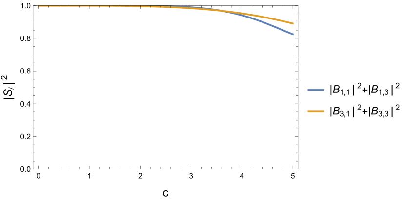
Figure 8: Contribution of $c=\delta\sqrt{\bar{\omega}^{2}-\bar{\mu}^{2}}$ to the normalization of $S_{\ell}$ functions

References

(1) R. D. Peccei and H. R. Quinn,
Phys. Rev. Lett. 38 (1977), 1440-1443.
(2) S. Weinberg,
Phys. Rev. Lett. 40 (1978), 223-226
(3) F. Wilczek,
Phys. Rev. Lett. 40 (1978), 279-282.
(4) P. Sikivie,
Phys. Rev. Lett. 51 (1983), 1415-1417
[erratum: Phys. Rev. Lett. 52 (1984), 695].
(5) R. Jackiw and S. Y. Pi,
Phys. Rev. D 68 (2003), 104012.
(6) L. Alvarez-Gaume and E. Witten,
Nucl. Phys. B 234 (1984), 269.
(7) S. L. Adler,
Phys. Rev. 177 (1969), 2426-2438.
(8) J. S. Bell and R. Jackiw,
Nuovo Cim. A 60 (1969), 47-61.
(9)
S. L. Detweiler,
Proc. Roy. Soc. Lond. A 352 (1977), 381-395.
(10) W. H. Press and S. A. Teukolsky, Nature 238, 211-212 (1972)
(11) T. Damour, N. Deruelle and R. Ruffini, Lett. Nuovo Cim. 15, 257-262 (1976).
(12) S. R. Dolan,
Phys. Rev. D 76 (2007), 084001.
(13) T. Fujita, I. Obata, T. Tanaka and K. Yamada,
Class. Quant. Grav. 38 (2021) no.4, 045010.
(14) For a recent discussion and references, see,
Y. S. Myung,
[arXiv:2208.14609 [gr-qc]].
(15) S. L. Detweiler,
Proc. Roy. Soc. Lond. A 349 (1976), 217-230
(16)
S. Alexander and N. Yunes,
Phys. Rept. 480 (2009), 1-55.
(17) T. Eguchi, P. B. Gilkey and A. J. Hanson,
Phys. Rept. 66 (1980), 213.
(18) S. A. Teukolsky,
Astrophys. J. 185 (1973), 635-647.
(19) Handbook of Mathematical Functions with Formulas, Graphs, and Mathematical Tables, edited bu M. Abramowitz and I. Stegun, pag. 751 (1968), Dover.
(20) R. A. Breuer , M. P. Ryan and S. Waller,
Proc Roy. Soc. 358, 71 (1977).
(21) C. Flammer, Spheroidal Wave Functions, Flammer, C. (Dover Publications, 2014.
(22) R. A. Isaacson,
Phys. Rev. 166 (1968), 1263-1271, ibid, Phys. Rev. 166 (1968), 1272-1279.
(23) S. Jung, T. Kim, J. Soda and Y. Urakawa,
Phys. Rev. D 102 (2020) no.5, 055013
doi:10.1103/PhysRevD.102.055013