Dark Energy Survey: Galaxy Sample for the Baryonic Acoustic Oscillation Measurement from the Final Dataset

Abstract

In this paper we present and validate the galaxy sample used for the analysis of the baryon acoustic oscillation (BAO) signal in the Dark Energy Survey (DES) Y6 data. The definition is based on a color and redshift-dependent magnitude cut optimized to select galaxies at redshifts higher than 0.6, while ensuring a high-quality photo-$z$ determination. The optimization is performed using a Fisher forecast algorithm, finding the optimal $i$-magnitude cut to be given by $i<19.64+2.894z_{\rm ph}$. For the optimal sample, we forecast an increase in precision in the BAO measurement of $\sim$25% with respect to the Y3 analysis. Our BAO sample has a total of 15,937,556 galaxies in the redshift range $0.6<z_{\rm ph}<1.2$, and its angular mask covers 4,273.42 deg² to a depth of $i=22.5$. We validate its redshift distributions with three different methods: directional neighborhood fitting algorithm (DNF), which is our primary photo-$z$ estimation; direct calibration with spectroscopic redshifts from VIPERS; and clustering redshift using SDSS galaxies. The fiducial redshift distribution is a combination of these three techniques performed by modifying the mean and width of the DNF distributions to match those of VIPERS and clustering redshift. In this paper we also describe the methodology used to mitigate the effect of observational systematics, which is analogous to the one used in the Y3 analysis. This paper is one of the two dedicated to the analysis of the BAO signal in DES Y6. In its companion paper, we present the angular diameter distance constraints obtained through the fitting to the BAO scale.

I Introduction

Baryon Acoustic Oscillations (BAO) is one of the most remarkable predictions of the formation of structures in the Universe [1, 2, 3, 4]. Since its first detection in 2005 [5], the measurement of the BAO scale has been one of the most important probes of dark energy, and also one of the main scientific drivers in the design and construction of galaxy surveys.

The BAO signal has already been detected many times in spectroscopic [6, 7, 8, 9, 10, 11, 12, 13, 14, 15, 16, 17, 18, 19] and photometric [20, 21, 22, 23, 24, 25, 26] datasets for galaxies, but also in the distribution of QSOs [27] and Lyman-$\alpha$ absorbers [28, 29], in a wide variety of redshifts, from $z=0.2$ to $z<3$. The estimation of the evolution of the BAO scale with time is a direct measurement of the expansion history of the Universe and, therefore, an excellent cosmology observable. All these measurements are compatible with the $\Lambda$CDM cosmological model.

In this context, the Dark Energy Survey (DES) [30, 31] aims to measure the BAO scale in the distribution of galaxies as one of its main objectives. In the DES Year 1 (Y1) analysis [25], we measured the BAO scale at an effective redshift of 0.81 with a sample that covered 1,336 deg². Because of this limited area, the detection had a low significance. On the other hand, in the DES Year 3 (Y3) analysis [26] we measured the BAO scale at an effective redshift of 0.835. The Y3 sample had a total of 7,031,993 galaxies, and covered 4,108.47 deg². Unlike in the case of the Y1, the significance of the detection in the Y3 was of about $3\sigma$ in the determination of the BAO feature. The BAO distance measurement obtained was $D_{M}(z_{\rm eff}=0.835)/r_{\rm d}=18.92\pm 0.51$ (where $D_{M}(z)$ is the comoving angular diameter distance and $r_{d}$ is the sound horizon scale), making it the most precise BAO distance measurement from imaging data alone ever (2.7% precision), and competitive with the latest transverse ones from spectroscopic samples at $z>0.75$. This result was consistent with Planck’s prediction at the level of $2.3\sigma$. In the DES Year 6 (Y6) analysis, i.e., the dataset analyzed here, we expect to measure the BAO feature at an effective redshift of 0.867 with 25% more precision compared to the Y3. Furthermore, this measurement will be combined with the other DES cosmological observables to estimate the most precise measurements on dark energy by combination of BAO with 3$\times$2pt (galaxy clustering + weak lensing) and type Ia supernovae, similarly to what we did in the Y3 analysis [26].

Detecting the BAO signal in photometric surveys poses a significant challenge due to the inherent smearing caused by the imprecise redshift determination. To mitigate this issue, it is crucial to identify a galaxy population exhibiting a distinctive spectral feature that can be captured using broadband filters. Generally, the preferred approach involves selecting old, well-evolved galaxies with a prominent $4000\text{\,}\mathrm{\text{Å}}$ break [32, 33, 34, 35]. This characteristic imparts a reddish appearance to the galaxies and often serves as the primary criterion for target selection in galaxy surveys.

In [34], we developed a color selection to choose galaxies in the DES Y1 analysis, calibrated through a set of synthetic SED distributions, optimized for redshifts $z>0.5$. This same color selection was the one used for the DES Y3 analysis, since we found it to be appropriate for the Y3 as well. In this new release, we re-optimize the Y1/Y3 sample selection. Also, since for the Y6 we have better data quality (deeper and more homogeneous) than for the Y3, i.e., less noisy magnitude estimations (because of the longer exposure time), we can afford going deeper in magnitude (and also in redshift), which allows us to go up to $z_{\rm ph}=1.2$ (compared to the $z_{\rm ph}=1.0$ limit of the Y1 analysis, or the $z_{\rm ph}=1.1$ limit of the Y3).

The structure of the paper is as follows: in subsection II.1 we present the parent DES Y6 data and the Directional Neighborhood Fitting algorithm [36], or DNF, which is the fiducial photo-$z$ code used within DES; in section III we describe the optimization of the DES Y6 BAO selection, together with the extra quality cuts we apply and its footprint; in section IV we present the validation of the redshift distributions of our optimal Y6 sample, for which we perform a direct calibration with VIPERS and also compare with the results from clustering redshift (WZ) using SDSS galaxies (the fiducial redshift distributions used in our analysis are a combination of DNF, VIPERS and WZ); in section V we describe the methodology used to mitigate the effect of observational systematics; and in section VII we show our conclusions to this analysis. The Y6 BAO sample will be eventually released at https://des.ncsa.illinois.edu/releases, together with all the other DES Y6 products.

In its companion paper [37], we perform the measurement of the BAO scale as a function of redshift, using the sample optimized here. We run the analysis in configuration and Fourier spaces (using the $w(\theta)$ and $C_{\ell}$ statistics, respectively), and also using the projected correlation function (PCF) estimator (using the $\xi_{p}(s_{\perp})$ statistics). Our fiducial measurement is the combination of the three estimators.

II DES Y6 Data

The operations of the Dark Energy Survey ended in 2019, after six years of data-taking. DES used the Blanco 4m telescope at Cerro Tololo Inter-American Observatory (CTIO) in Chile, and observed $\sim$5000 deg² of the southern sky in five broadband filters (bands), $grizY$, ranging from $\sim$400 nm to $\sim$1060 nm [38, 39], using the DECam [40] camera. Its images were processed with the DES Data Management system hosted at NCSA, coadded on colocated points in the sky for each band, from which catalogs of objects are produced using the combined detection in $riz$ bands [41]. These final catalogs have been released as the public Data Release 2 of the project [42].

II.1 Gold Catalog

The coadd catalog is further enhanced into a Y6 Gold catalog [43]. This is a value-added data product that includes additional columns and other ancillary data such as survey property maps, that were not included in DR2, but are used for galaxy clustering analyses for Y6 data among other applications. This catalog is the basis of the BAO sample, in particular the 2.1 version. A short summary of the main features of Y6 Gold relevant to the BAO sample is provided below.

A more robust and precise photometry estimate:

Flux measurements in Y6 employ a bulge plus disk model for the fit across epochs and bands, with masking of nearby objects (using the code fitVD, see Section 3 of [44] for a description). As a change with respect to the Y3 Gold approach, the bulge and disk size ratio has been fixed in order to improve the robustness of the measurement and reduce uncertainties in the derived parameters.

An improved star-galaxy classifier:

The quantity EXT_MASH measures the deviation of an object from a point-like source using 5 categories ranging from 0 (most point-like) to 4 (most extended-like). These categories are created as regions in the size (BDF_T) vs signal-to-noise (BDF_S2N) space of the fitvd quantities of the Y6 Gold photometry. In those cases where fitvd is not available, we use SExtractor variables (see [42]).

Additional quality flags:

The column FLAGS_GOLD is a bitmask that summarizes a collection of flags coming from the detection and measurement algorithms, and at the same time adds specific features of DES images that have shown up during the years, to avoid including them in standard analyses.

A pixelized footprint mask with detection fraction information:

An angular mask in HEALPix format containing a positive value for a given pixel if

1. it has, at least, 2 exposures in each of the $griz$ bands.

2. it covers, at least, 50% of the HEALPix combined $griz$ coverage area.

This value is equal to the combined $griz$ coverage area, determined by a higher resolution subpixelization. In addition, each object has a FLAGS_FOOTPRINT value with this information as well, and at the same time an assurance that the object has been indeed observed through the NITER_MODEL variable in $griz$.

An astrophysical foregrounds mask:

The Y6 Gold data set incorporates a mask that selects regions marked as having potentially problematic astrophysical foregrounds, such as bright stars from the 2MASS catalog, large nearby galaxies or extended globular clusters and dwarf spheroidals. This mask is incorporated into the angular mask used to select the BAO sample and estimate the galaxy clustering, as described in subsection III.1.

Survey property maps:

The Y6 Gold survey property maps are data structures that track the spatial distribution on sky of specific observation characteristics or astrophysical measurerements, which might impact the detectability of sources and their features. We use these maps (in HEALPix format) to reduce the effect of systematic errors on galaxy clustering, as described in [45] and detailed for Y6 data in section V.

A photometric redshift estimate:

In Y6, the fiducial photometric redshift estimate is DNF, which is described in subsection II.2.

The Y6 Gold catalog version used for this analysis corresponds to the internal release version 2.1, which has some minor differences with the upcoming public released Y6 Gold catalog (version 2.2). These differences include:

• In Y6 Gold version 2.1, the fitvd photometry used in the DNF estimates is slightly modified (O(mmag)) with respect to the photometry in the tables, corresponding to small differences in photometric corrections applied to the magnitudes.

• In Y6 Gold version 2.1, the DNF estimates include the Y band, to ensure better coverage at higher redshift. At the same time, the robustness of the measurement is more insensitive to Y band survey property systematics (section V).

• In Y6 Gold version 2.1, the FLAGS_FOOTPRINT flag includes detection fraction information, which is separated in subsequent versions into footprint binary mask and survey property detection fraction mask.

• In Y6 Gold version 2.1, an additional masking on three particular tiles that had corrupt flux values was added, totalling $\sim 1.5$ square degrees.

II.2 DNF Redshifts

In order to assign galaxies to each redshift bin, we use the photo-$z$ estimate given by the Directional Neighborhood Fitting (DNF) algorithm [36], which was trained using $grizY$ magnitudes onto a large spectroscopic reference sample. DNF is a non-parametric method that uses a training set of galaxies with known spectroscopic redshifts to establish the relationship between the observed magnitudes and the true redshifts. The training set, compiled and validated in [46], is described in [43].

DNF works by fitting a linear function in the neighborhood (magnitude-color space) to the target galaxy within the training set, where the function predicts the redshift of a galaxy based on its magnitudes. The key point of DNF is that it takes into account the fact that the relationship between magnitudes and redshift may vary in different regions of the magnitude-color space. The algorithm defines a “direction” in the magnitude-color space to look for neighbors on the training set, and thus it fits a different linear function of magnitudes for each galaxy. This allows DNF to capture more complex relationships between magnitudes-colors and redshift than other methods [36].

DNF predicts the point-estimate of the photo-$z$ (called DNF_Z in the DES catalogs), as well as the redshift of the closest neighbor (DNF_ZN) and the full PDF distribution. The photo-$z$ estimate DNF_Z is computed as

$$z_{\rm ph}\equiv\textsc{DNF\_Z}=\sum_{i}\bm{a}_{i}\cdot\bm{m}_{i},$$ (1)

where $i$ denotes a sum over magnitudes, $\bm{a}_{i}$ is a parameter vector and $\bm{m}_{i}$ are the magnitudes in the different bands. The vector $\bm{a}_{i}$ is obtained by fitting the linear function using a least square regression to the set of neighbors considered. Later, DNF_Z is used to assign galaxies to the redshift bins used in our BAO analysis.

III Sample Selection

As we mentioned earlier, the same sample selection was used for both the Y1 and the Y3 BAO analyses, namely

$$1.7<i-z+2(r-i) \text{(color selection)},$$ (2)

$$17.5<i<19+3z_{\rm ph} \text{(flux selection)},$$

$$0.6<z_{\rm ph}<z_{\rm ph}^{\rm max} \text{(photo-$z$ range)},$$

where $r$, $i$ and $z$ are the magnitudes in the $riz$ bands, respectively; $z_{\rm ph}$ is the photometric redshift, which is given by DNF_Z (as defined in subsection II.2); and $z_{\rm ph}^{\rm max}$ is the maximum photometric redshift.

1. Color selection. The color selection of Equation 2 was defined during the Y1 BAO analysis in order to select galaxies beyond $z_{\rm ph}=0.5$, following the spectral energy distribution (SED) for elliptical galaxies. Further details about this selection cut can be found in Fig. 5 of [34], where we estimated the colors of a set of SED templates as a function of redshift seen through the DES filter pass-bands. We used the same one for the Y3 analysis, and we adopt it for the Y6 as well.

2. Flux selection. In this work we re-optimize the flux selection of Equation 2. To do so, we leave the intercept on the y-axis and the slope as free parameters, i.e.,

   $$17.5<i<a+bz_{\rm ph}.$$ (3)

3. Photo-$z$ range. The maximum redshift, $z_{\rm ph}^{\rm max}$, was 1.0 for the Y1 and 1.1 for the Y3. For the Y6, it will be set to 1.2.

Besides these selection cuts, by default we apply the following quality cuts to the Y6 Gold catalog:

$$\textsc{EXT\_MASH}\geq 3,$$ (4)

$$\textsc{FLAGS\_GOLD}=0,$$

$$\textsc{N\_IMAGES}\_[{\rm GRIZY}]>1.$$

EXT_MASH and FLAGS_GOLD were already defined in subsection II.1. N_IMAGES_[GRIZY] is the number of $grizY$ band exposures at the object location (from the HEALPix map). All these flags are described in more detail in [43].

III.1 Angular Mask

The angular mask is constructed similarly to the one we used for the Y3 analysis, see [45]. In order to build it, we required:

1. pixels must be in the Y6 Gold footprint (see subsection II.1) and have an effective coverage $>80\%$.

2. pixels must not be affected by foreground sources, like regions around bright stars or extended galaxies.

3. pixels must have a $10\sigma$ depth in $i$ greater than 22.5.

The resultant footprint is shown in Figure 1, showing the $i$-band depth in each pixel. It is worth mentioning that this is the parent mask, not the final mask, from which our BAO sample is made.

Figure 1: Footprint for the DES Y6 data. Each pixel is colored as a function of its depth in the $i$ band. The total area of the footprint considering the detection fraction of each pixel is 4,374.20 deg².

Different to the previous release, for the Y6 analysis we aim to optimize the sample selection as a function of the $i$-magnitude cut, see Equation 3. Therefore, it is necessary to carefully account for the depth maps related to our footprint. Each pixel plotted in Figure 1 reaches a different depth in the $i$ band, which effectively limits the area of the mask as a function of the $i$-magnitude cut that we set, $i_{\rm max}$. In Figure 2 we show the area of the angular mask as a function of this $i_{\rm max}$. The deeper we want our sample to be, the more area of the full footprint we need to remove. The orange dashed line shown in this figure corresponds to the Y3 $i$-magnitude limit, which was simply $i_{\rm max}=19+3z_{\rm ph}^{\rm max}=19+3\times 1.1=22.3$ (directly computed using $z_{\rm ph}^{\rm max}=1.1$). The green dashed line corresponds to the $i$-magnitude limit chosen for the Y6, which will be set to 22.5. The area of such mask is 4,357.01 deg², which can be compared with the total area of the original angular mask, which is 4,374.20 deg²: we conclude that we barely lose any area by setting the $i=22.5$ limit. The final version of the Y6 BAO angular mask will have a slightly smaller area, 4,273.42 deg² (see subsection III.3 for further details).

Since for the Y6 we have better data quality than for the Y3, i.e., less noisy magnitude estimations (because of the longer exposure time), we can afford going deeper in magnitude (and also in redshift). However, we cannot arbitrarily go to higher magnitudes: first, because we would lose area; second, because photo-$z$ precision worsens as magnitude increases in the faint limit; and third, galaxies would be more affected by observational systematics. In order to mitigate the impact from redshift uncertainties and inaccuracies, we choose to limit our sample to

$$i<22.5.$$ (5)

The reason to choose this particular value is that we do not have reference spectra for fainter galaxies, i.e., we would not be able to trust and/or validate the photo-$z$ of a fainter galaxy sample. In fact, to calibrate the photometric redshifts in section IV we use VIPERS, which is a complete spectroscopic sample above redshift 0.5, but only up to $i<22.5$ (see [47] for further details).

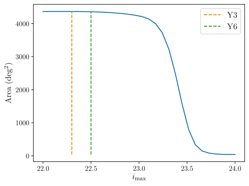
Figure 2: Area of the Y6 footprint mask as a function of the $i$-magnitude limit (blue solid line). The orange dashed line indicates the limit for the Y3 analysis ($i_{\rm max}=22.3$), whereas the green dashed line represents the same but for the Y6 ($i_{\rm max}=22.5$). We find that we barely lose any area after applying the $i=22.5$ cut (we still have 4,357.01 deg² from the total of 4,374.20 deg²).

III.2 Optimization of the Selection Cuts

III.2.1 Forecast Method

The forecasting method we use is based upon the methodology developed in [48]. Following [48, 49] and assuming the likelihood function of the band powers of the galaxy power spectrum to be Gaussian, the Fisher matrix can be approximated as

$$F_{ij} =\int_{\bm{k}_{\rm min}}^{\bm{k}_{\rm max}}\frac{d^{3}\bm{k}}{2(2\pi)^{3}}V_{\rm eff}(\bm{k})\frac{\partial\log P_{G}(\bm{k})}{\partial p_{i}}\frac{\partial\log P_{G}(\bm{k})}{\partial p_{j}}$$

$$=\int_{-1}^{1}d\mu\int_{k_{\rm min}}^{k_{\rm max}}\frac{2\pi k^{2}dk}{2(2\pi)^{3}}V_{\rm eff}(k,\mu)$$

$$\qquad\times\frac{\partial\log P_{G}(k,\mu)}{\partial p_{i}}\frac{\partial\log P_{G}(k,\mu)}{\partial p_{j}}.$$ (6)

$P_{G}(\bm{k})$ is the observed galaxy power spectrum at $\bm{k}$, $\mu$ is the cosine of the angle of $\bm{k}$ with respect to the line of sight (LOS), $p_{i}$ are the cosmological parameters to be constrained, and $V_{\rm eff}$ is the effective volume of the survey, given by

$$V_{\rm eff}(k,\mu)=\int d^{3}\bm{r}\left[\frac{n_{\rm gal}(\bm{r})P_{G}(k,\mu)}{n_{\rm gal}(\bm{r})P_{G}(k,\mu)+1}\right]^{2}$$

$$=\left[\frac{(1+\beta\mu^{2})^{2}P(k)}{(1+\beta\mu^{2})^{2}P(k)+n_{\rm gal}^{-1}}\right]^{2}V_{\rm survey}.$$ (7)

Here, $n_{\rm gal}(\bm{r})$ is the comoving number density of galaxies (that we assumed constant in angular position) and $\beta$ is the linear redshift-space-distortion parameter. Also, $V_{\rm survey}$ is given by

$$V_{\rm survey}=\frac{4\pi}{3}f_{\rm sky}\left[\chi(z_{\rm max})^{3}-\chi(z_{\rm min})^{3}\right].$$ (8)

This Fisher matrix can then be approximated based on how well we can center the location of the baryonic peak, i.e., the sound horizon scale $s_{o}$ at the drag epoch when observed in the reference cosmology. Following [48], the fractional error on the location of the peak can be written as

$$\sigma_{\log s_{o}}=\frac{\sigma_{s_{o}}}{s_{o}}=\sqrt{F^{-1}_{\log s_{o}}}=\left\{V_{\rm survey}A_{0}^{2}\int_{k_{\rm min}}^{k_{\rm max}}dk\right.$$

$$\left.\times\frac{k^{2}\exp\left(-2(k\Sigma_{\rm Silk})^{1.4}\right)\exp\left(-2k^{2}\Sigma_{\rm tot}^{2}\right)}{\left(\frac{P(k)}{P_{0.2}}+\frac{1}{n_{\rm gal}P_{0.2}}\right)^{2}}\right\}^{-1/2},$$ (9)

where $A_{0}$ is a constant factor normalizing the baryonic power spectrum [48], $P_{0.2}$ is the galaxy power spectrum at $k=0.2$ $h$/Mpc at the given redshift and the factors $\Sigma_{\rm Silk}$ and $\Sigma_{\rm tot}$ give the broadening of the BAO peak with a Gaussian function due to the Silk damping effect and the Lagrangian displacement, respectively. From Equation 9 it follows that the distance precision depends only on the survey volume, the number density of galaxies and the redshift of the survey. However, for photometric redshift surveys such as DES it also depends on the width of the photo-$z$ distribution, $\Sigma_{z}$, since photometric redshift errors result in an exponential suppression of the power spectrum,

$$P\to P\exp(-k^{2}\mu^{2}\Sigma_{z}^{2}).$$ (10)

$\sigma_{\log s_{o}}$ is equivalent to the fractional error on the distance estimation when the physical location of the peak is well known from the CMB [48]. We compute it for each redshift bin and then combine these as

$$\sigma_{\rm BAO}=\left[\sum_{\rm zbin}\frac{1}{(\sigma_{\log s_{o}}^{\rm zbin})^{2}}\right]^{-1/2}.$$ (11)

In order to run the forecasts, we need:

• $z_{\rm min}$ and $z_{\rm max}$.

• the area of the angular mask, $A_{\rm mask}$, which depends on the $i$-magnitude limit of the sample (see Figure 2). It allows us to compute $f_{\rm sky}$.

• the value of $\Sigma_{z}$ for each individual redshift bin (calculated using the expression given in Appendix A).

• the number of galaxies, $N_{\rm gal}$, in each redshift bin, from which we compute the number density as

  $$n_{\rm gal}=\frac{N_{\rm gal}}{A_{\rm mask}}.$$ (12)

III.2.2 Optimization Algorithm

Here we describe the algorithm developed to optimize the sample selection. We first run the algorithm in 5-bin samples with photo-$z$ between 0.6 and 1.1, and then extend the analysis to 6-bin samples with photo-$z$ between 0.6 and 1.2.

In order to optimize the sample selection for the best BAO scale measurement, we need to include, at least, one free parameter in our sample selection. We add this freedom in the flux selection leaving the slope and the intercept on y-axis as free parameters: $17.5<i<a+bz_{\rm ph}$, as we discussed earlier (the other cuts are fixed by the survey characteristics). Setting $a=19$ and $b=3$ corresponds to the Y3 selection, Equation 2. As mentioned earlier, we impose an extra cut requiring $i<22.5$, Equation 5. We allow $a$ and $b$ to vary in the ranges

$$19\leq a\leq 22,\quad 1.5\leq b\leq 3.5,$$ (13)

with 100 linearly-spaced values in each interval (for a total of 10,000 test samples), in order to search for their optimal values. The optimization algorithm works as follows:

1. Select a pair of values for $a$ and $b$.

2. Compute $i_{\rm max}=\text{min}(a+bz_{\rm ph}^{\rm max},22.5)$, where $z_{\rm ph}^{\rm max}=1.1$. By default, we set the $i$-magnitude limit to 22.5. However, depending on the values of $a$ and $b$, for some samples $a+bz_{\rm ph}^{\rm max}<22.5$ and, therefore, we would unnecessarily lose area for them if we simply set $i_{\rm max}=22.5$. Therefore, the correct way to compute $i_{\rm max}$ for a given sample is to calculate the minimum between $a+bz_{\rm ph}^{\rm max}$ and 22.5.

3. Remove pixels with depth in the $i$-magnitude band smaller than $i_{\rm max}$ from the angular mask. Compute the total area of the remaining pixels, taking into account the detection fraction of each of them. This step implies using a different angular mask for each sample (as a function of the value of $i_{\rm max}$).

4. Create a galaxy sample applying the Y6 quality cuts, defined by Equation 4, and also the corresponding selection cuts to the Y6 Gold Catalog.

5. Compute $\sigma_{68}$ and count the number of galaxies $N_{\rm gal}$ in each redshift bin for the galaxy sample created in step 4.

6. Compute $\sigma_{\rm BAO}$ with the Fisher forecast code using the area of the angular mask (computed in step 3.), $\sigma_{68}$ and $N_{\rm gal}$ (both of them computed in step 4.), as explained in subsubsection III.2.1.

We apply this algorithm to the grid in the $(a,b)$ plane defined by Equation 13 and find that the minimum value for $\sigma_{\rm BAO}$ is

$$\sigma_{\rm BAO}^{\rm Y6-opt}=0.0170.$$ (14)

The corresponding optimal parameters are $a=19.64$ and $b=2.894$, which are well within the limits of the $(a,b)$ plane we previously defined.

As already mentioned, Y6 photometric redshifts are more accurate, and therefore we can further optimize the BAO sample by increasing the photo-$z$ range, i.e., adding one more redshift bin from 1.1 to 1.2. We run the forecasts in the same $(a,b)$ plane as before, and find that the minimum value for $\sigma_{\rm BAO}$ is

$$\sigma_{\rm BAO}^{\rm Y6-opt}=0.0162,$$ (15)

which is smaller than the minimum value for the 5-bin case displayed in Equation 14, i.e., $\sigma_{\rm BAO}$ decreases when adding one extra redshift bin, as expected. The optimal parameters found for the 6-bin case are exactly the same as the ones we found for the 5-bin one, namely

$$a_{\rm Y6-opt}=19.64,$$ (16)

$$b_{\rm Y6-opt}=2.894,$$

i.e., adding one extra redshift bin does not impact the optimal values for $a$ and $b$.

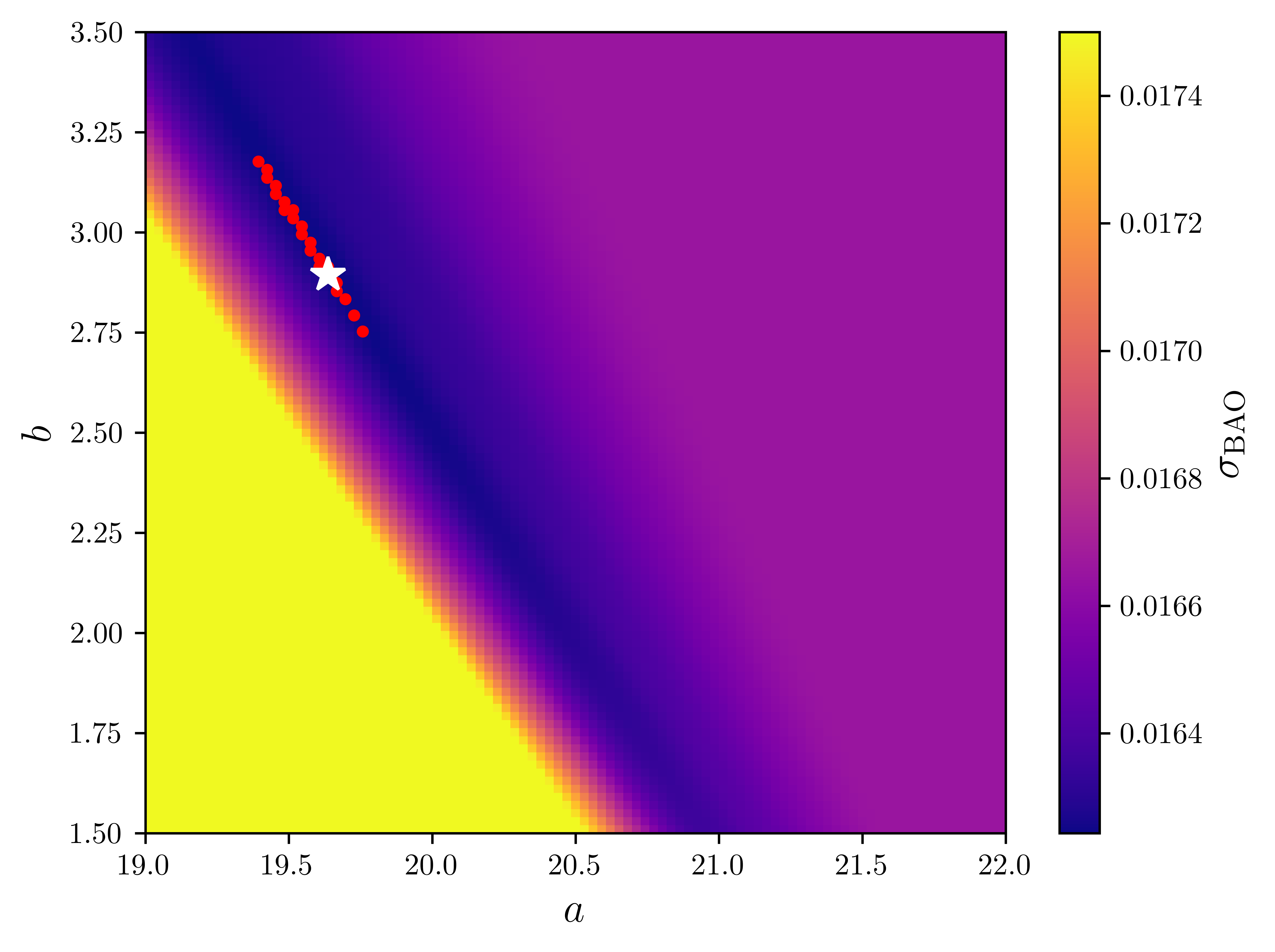
Figure 3: Heat-map of $\sigma_{\rm BAO}$ obtained for samples selected with different values of $a$ and $b$ following Equation 3. The white star represents the sample with the lowest $\sigma_{\rm BAO}$, whereas the red points correspond to the next 20 samples with lower values for this variable. The optimal sample has $a=19.64$ and $b=2.894$, and a value of $\sigma_{\rm BAO}=0.0162$.

In Figure 3 we show the $\sigma_{\rm BAO}$ heat-map obtained from the forecasts as a function of $a$ and $b$. The sample with the lowest $\sigma_{\rm BAO}$ is shown as a white star, but we also include the next 20 samples with the lowest values of $\sigma_{\rm BAO}$ as red points. We find that all of them lie in a diagonal-like region in which the forecasted error reaches its minimum value, i.e., all the samples in this region have, approximately, the same $\sigma_{\rm BAO}$. We studied several properties for all these samples: the width of the photo-$z$ distribution, the total number of galaxies, the limiting magnitude and the number of photo-$z$ outliers. However, we did not find any significant difference between them: all their properties were quite similar. Therefore, we decided to choose the values of $a$ and $b$ corresponding to the sample with the lowest $\sigma_{\rm BAO}$, i.e., the ones displayed in Equation 16. Therefore, the final selection of the Y6 sample is given by

$$1.7<i-z+2(r-i),$$ (17)

$$17.5<i<19.64+2.894z_{\rm ph},$$

$$i<22.5,$$

$$0.6<z_{\rm ph}<1.2.$$

In Table 1 we summarize the results of the forecast applied to several different samples. We include the results for the Y3 BAO sample, a Y6 sample selected using the Y3 cuts with 5 and 6 redshift bins (i.e., applying Equation 2 with $z_{\rm ph}^{\rm max}=1.1$ and 1.2, respectively), and the Y6 optimal sample with 5 and 6 redshift bins. We note that the 6-bin cases always improve with respect to the 5-bin ones. We also find that the optimal 5-bin case is already better that the Y3-selection-like 6-bin one (forecasted errors of 1.70% and 1.76%, respectively). The lowest value of $\sigma_{\rm BAO}$ corresponds to the 6-bin optimal Y6 sample, as expected. From these numbers, we conclude that we expect the error associated to the BAO distance measurement to be reduced by about a 25% with respect to the Y3 analysis, i.e., it goes from 2.14% to 1.62%, which is an important increase in precision. Part of this increase in precision is due to the higher quality of the Y6 data (2.14% to 1.85%), part is due to the optimization of the selection cuts (1.85% to 1.70%) and part is due to the increase in redshift (1.70% to 1.62%).

Case	$\sigma_{\rm BAO}$
Y3	0.0214
Y6-Y3sel (5 redshift bins)	0.0185
Y6-Y3sel (6 redshift bins)	0.0176
Y6-opt (5 redshift bins)	0.0170
Y6-opt (6 redshift bins)	0.0162

Table 1: Summary of the results of the Fisher forecast code applied to different samples. We include the cases of running the code using the properties of the Y3 sample; those of the Y6 sample selected with the same selection cuts as in the Y3 (5 and 6 redshift bins); and also those of the optimal Y6 sample (5 and 6 redshift bins). As expected, the most precise sample to measure the BAO feature is the optimal one with 6 redshift bins (highlighted case).

III.3 Improvement of the Quality Cuts

In order to remove objects with large magnitude errors, additional magnitude cuts were imposed to the selection, which in consequence produced poor photo-$z$ estimates. In average, these cuts ensure that galaxies have a signal-to-noise ratio greater than 3 in $grz$ bands:

$$g<25.5,$$ (18)

$$r<25,$$

$$z<24.$$

The star-galaxy separator was modified from the original $\textsc{EXT\_MASH}\geq 3$, see Equation 4, to $\textsc{EXT\_MASH}=4$, which proved to better remove the remaining stellar contamination. The Y6 BAO mask was also slightly modified in order to remove regions with globular clusters and image artifacts, as detailed subsection V.1. The final mask has an area of 4,273.42 deg². Around $5\%$ of the galaxies of the Y6 optimal sample were removed with the combined effect of applying the new quality cuts and the modified angular mask.

In Table 2 we display the properties of the final version of the Y6 BAO sample. We find that in the Y6 analysis we have, approximately, doubled the number of galaxies in our sample with respect to the Y3 [50]. The main reason for this is the new $i$-magnitude limit of $i<19.64+2.894z_{\rm ph}$ vs $i<19+3z_{\rm ph}$ in Y3, which allows us to go deeper in every redshift bin, e.g., $i<21.67$ in the first redshift bin for Y6 vs $i<21.1$ in the Y3.

Bin	$N_{\rm gal}$	$\sigma_{68}$
$0.6<z_{\rm ph}<0.7$	2,854,542	0.0232
$0.7<z_{\rm ph}<0.8$	3,266,097	0.0254
$0.8<z_{\rm ph}<0.9$	3,898,672	0.0292
$0.9<z_{\rm ph}<1.0$	3,404,744	0.0358
$1.0<z_{\rm ph}<1.1$	1,752,169	0.0403
$1.1<z_{\rm ph}<1.2$	761,332	0.0415

Table 2: Main properties of the Y6 BAO sample as a function of redshift: number of galaxies and dispersion on the photo-$z$, computed using DNF_ZN and DNF_Z as described in Appendix A. The sample covers 4,273.42 deg², with a total of 15,937,556 galaxies. The effective redshift of the sample is $z_{\rm eff}=0.867$, as computed in [37].

IV Redshift Calibration

In this section we validate the redshift distributions of our BAO sample. Even though we could just use the VIPERS Z_SPEC values for this (spectroscopic complete sample within our redshift/magnitude selection), we supplement them with the redshift distributions estimated using clustering redshifts (WZ). Both these methods produce somewhat noisy redshift distributions, which is the reason why we use the smoother DNF redshift distributions as templates and shift and stretch them with respect to these two as our fiducial choice (which we label as “fiducial” throughout this paper). This section is divided into three subsections: in subsection IV.1, we perform a direct calibration of our photometric redshifts using VIPERS; in subsection IV.2, we estimate the redshift distributions using the WZ technique; and in subsection IV.3, we describe the algorithm developed to shift and stretch the DNF redshift distributions to make them match the properties of VIPERS Z_SPEC and WZ.

In Figure 4 we show the redshift distributions for all the different methods we just mentioned. DNF provides two alternative estimations of the redshift distributions: $n(\textsc{DNF\_ZN})$ and PDF. The first one is obtained as histograms of DNF_ZN in redshift bins defined by DNF_Z, whereas the second one is obtained as the stacking of individual galaxy PDFs [36]. These two are shown in Figure 4 as blue histograms and green lines, respectively. We find that the distributions of DNF_ZN are quite smooth, being the last redshift bin the noisiest one. This is somewhat expected, since the last redshift bin is the one with the lowest number density, and also the one for which it is more complicated to estimate the photo-$z$ (there are fewer galaxies in the spectroscopic training sample at higher redshifts). The combination of these two effects yield to a decrease in the photo-$z$ quality at such high redshifts, and also makes the redshift distributions noisier. On the other hand, we find that DNF PDF is qualitatively similar to DNF_ZN, but smoother (since it is computed as the stacking of large amounts of individual galaxy PDFs). Besides the DNF results, in Figure 4 we also include the redshift distributions of VIPERS Z_SPEC, WZ and the fiducial choice, which are further discussed later.

In Table 3 we show the mean and width of the different redshift distributions shown in Figure 4. The results shown in this table were computed with the expressions given in Appendix A, and are plotted in Figure 5 for visualization purposes. We find that the properties of DNF_ZN and DNF PDF are quite similar. Also, those of VIPERS Z_SPEC and WZ are in very good agreement. It is also important noting that both DNF_ZN and DNF PDF are biased and wider with respect to Z_SPEC and WZ, which is the reason why we cannot use directly the results from DNF as the redshift distributions of our sample (and the reason why we will shift and stretch them to match the properties of VIPERS and WZ, which are closer to the underlying true redshift distributions).

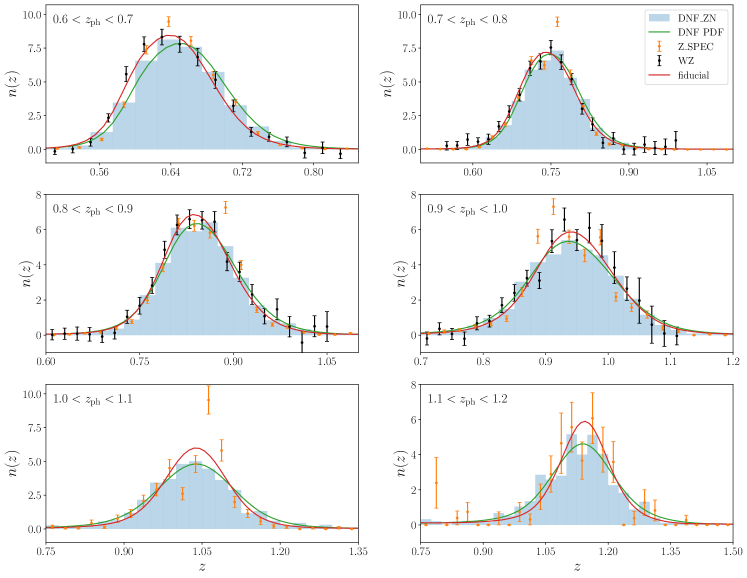
Figure 4: Redshift distributions of the Y6 BAO analysis. In the case of DNF, we show both DNF_ZN and the stacking of DNF PDF (blue histograms and green lines, respectively). We also include the distributions of VIPERS Z_SPEC (orange points with error-bars), WZ (black points with error-bars) and the fiducial choice (red lines), which corresponds to the redshift distributions of DNF PDF but shifted and stretched with respect to WZ in the first 4 redshift bins, and with respect to VIPERS Z_SPEC in the last 2, following the methodology described in subsection IV.3. The mean and width of all these redshift distributions (computed using the expressions given in Appendix A) are displayed in Table 3, and plotted in Figure 5.

Bin	$\langle z\rangle$					$W_{68}$
	DNF_ZN	DNF PDF	Z_SPEC	WZ	fiducial	DNF_ZN	DNF PDF	Z_SPEC	WZ	fiducial
$0.6<z_{\rm ph}<0.7$	0.654	0.658	0.650	0.644	0.646	0.050	0.051	0.045	0.047	0.047
$0.7<z_{\rm ph}<0.8$	0.752	0.754	0.746	0.743	0.747	0.058	0.057	0.050	0.057	0.056
$0.8<z_{\rm ph}<0.9$	0.844	0.847	0.849	0.848	0.842	0.063	0.065	0.056	0.059	0.060
$0.9<z_{\rm ph}<1.0$	0.929	0.934	0.931	0.941	0.938	0.077	0.079	0.061	0.066	0.071
$1.0<z_{\rm ph}<1.1$	1.013	1.020	1.023	—	1.023	0.086	0.089	0.067	—	0.071
$1.1<z_{\rm ph}<1.2$	1.107	1.111	1.111	—	1.122	0.093	0.096	0.077	—	0.075

Table 3: Mean and width of the redshift distributions, computed using the expressions given in Appendix A, for DNF_ZN, DNF PDF, VIPERS Z_SPEC, WZ and the fiducial choice.

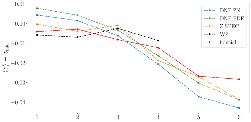
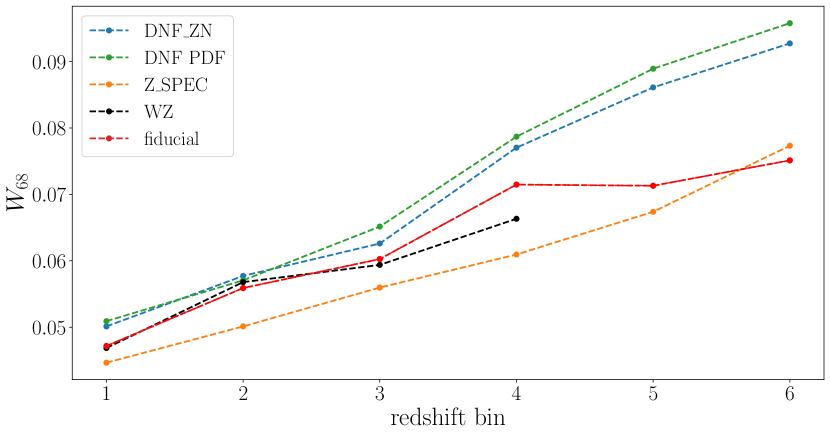
Figure 5: Top panel: average redshift of the different redshift distributions of the Y6 analysis. For visualization purposes, we subtracted the middle redshift, which is given by the average of the limits for each redshift bin (0.65, 0.75, 0.85, 0.95, 1.05 and 1.15, respectively). Bottom panel: width of the different redshift distributions of the Y6 analysis. Cases included in this plot: DNF_ZN (blue), DNF PDF (green), Z_SPEC (orange), WZ (black) and fiducial choice (red).

IV.1 Direct Calibration with VIPERS Spectroscopic Redshifts

We calibrate our photo-$z$ using VIPERS, similarly to what we did during the Y3 BAO analysis [50]. VIPERS is a complete spectroscopic sample for redshifts above 0.5 and up to $i=22.5$, see [47] (the same $i$-magnitude limit we set for our BAO sample), with an overlapping area of 16.3 deg² with DES. Therefore, the distributions of the spectroscopic redshifts of VIPERS in redshift bins defined by DNF_Z provide a direct estimation of the true redshift distributions of our BAO sample (this is explicitly shown in Appendix B). These distributions are plotted as orange points with error-bars in Figure 4.

One caveat is that, due to the small overlap between VIPERS and DES, the Z_SPEC distributions are noisy, particularly in the last two redshift bins. Also, as we mentioned earlier, the distributions of Z_SPEC are narrower than those from DNF (see Table 3). For these two reasons, we use Z_SPEC to shift and stretch the DNF redshift distributions for redshifts above 1.0. For redshifts below 1.0, we use clustering redshift, which we describe next.

IV.2 Clustering Redshift (WZ)

There are alternative ways to estimate the redshift distributions of our BAO sample, such as the clustering redshift technique [51]. Clustering redshifts make use of the fact that galaxies with unknown redshifts reside in the same structures as galaxies that have known redshifts. Thus, spatial cross-correlations can be used to estimate the redshift distribution of the sample with unknown redshifts. The modern approach of using this data to obtain a precise estimate of a redshift distribution can be traced back to [51]. Since then, it has been implemented and further developed in the literature, see [52, 53, 54, 55, 56, 57, 58, 59] for reference. This technique was already validated and applied to the Y3 MagLim sample in order to calibrate its redshift distributions in [60], and we use the methodology choices from that work. In that case and also in this one, spectroscopic galaxies from BOSS [61] and its extension, eBOSS [62, 63], are used to cross-correlate with our sample. These samples overlap about 15% of the DES footprint.

In Figure 4 we show the redshift distributions for WZ (black points with error-bars). Because of the lack of spectroscopic galaxies in the redshift range $1.0<z<1.2$, it was not possible to estimate them for the last two bins. We find that WZ is consistent with Z_SPEC, see the results displayed in Table 3. Since we have two independent determinations of the redshift distributions that agree, i.e., VIPERS Z_SPEC and WZ, we consider them as validated.

As in the case of Z_SPEC, WZ is also somewhat noisy. To address the problem of the noisy nature of WZ and VIPERS Z_SPEC, for the fiducial analysis on the data we decided to use a modified version of the DNF redshift distributions as our default choice: shifted and stretched to match the properties of WZ in the first 4 redshift bins and Z_SPEC in the last 2. Therefore, DNF $n(z)$ are used as templates for the shape of our fiducial redshift distributions.

IV.3 Shift and Stretch Algorithm

Here we describe the algorithm developed to perform the shift and stretch of DNF_ZN and DNF PDF. We run the shift and stretch of a given $n(z)$ in two different steps:

1. Shift of the original $n(z)$. The shifted redshift distribution is, simply, given by

   $$n_{\rm shifted}(z,\Delta z)=n(z-\Delta z).$$ (19)

2. Stretch of the shifted $n(z)$. The shifted and stretched redshift distribution is given by

   $$n_{\rm 2-param}(z,\Delta z,\sigma_{z})$$

   $$=n_{\rm shifted}(\sigma_{z}(z-\langle z\rangle_{\Delta z})+\langle z\rangle_{\Delta z},\Delta z),$$ (20)

   where

   $$\langle z\rangle_{\Delta z}\equiv\int dz\hskip 1.42271ptn_{\rm shifted}(z,\Delta z).$$ (21)

We, then, compute the best fit parameters $\Delta z$ and $\sigma_{z}$ by minimizing

$$\chi^{2}(\Delta z,\sigma_{z})=\sum_{i}\left[\frac{n_{\rm 2-param}(z_{i},\Delta z,\sigma_{z})-n_{\rm ref}(z_{i})}{\Delta n_{\rm ref}(z_{i})}\right]^{2}.$$ (22)

Since the redshift distributions we shift and stretch are either DNF_ZN or DNF PDF, we neglect their contribution to the denominator of the previous expression, since their shot-noise is much smaller than that of the reference redshift distribution, which is either VIPERS or WZ. This methodology is similar to the one used for the DES Y3 3$\times$2pt analysis, see [64]. In that context, these shift and stretch parameters appear because of our uncertainty in the photo-$z$, and this implementation is particularly useful since it allows us to fit for them when running the 3$\times$2pt chains.

Using the algorithm we just described, we perform the shift and stretch of DNF PDF with respect to WZ in the first 4 redshift bins, and with respect to Z_SPEC in the last 2. The resulting redshift distributions are shown as red lines in Figure 4, where we can check that they are as smooth as the original DNF PDF, but shifted and stretched. From the results displayed in Table 3, we find that the fiducial choice has similar mean and width to those of WZ in the first 4 redshift bins and to those of Z_SPEC in the last 2, as intended. These are the redshift distributions used to generate the BAO template to run the BAO fits on the data in [37].

For the projected correlation function (PCF) estimator that we use to measure the BAO in [37], the shift and stretch algorithm is adapted to work in 22 logarithmic redshift bins, instead of the fiducial 6 redshift bins. This is described in Appendix C.

V Correcting for Observational Systematics

In order to reduce the impact of observational systematics, we apply two complementary strategies: we first mask pixels with potentially problematic values and, next, we compute correcting weights that are applied to our galaxy sample. Both steps rely on survey property (SP) maps, which are pixel maps that keep track of spatial variations of the different systematic effects concerning the imaging of the data. Among these SP maps we consider effects such as the seeing (FWHM) and the limiting magnitude, but also astrophysical foregrounds, such as contamination from the stellar density and galactic dust extinction.

V.1 Masking Observational Systematics

As a first step to mitigate the impact of observational systematic effects, we apply an angular mask to our galaxy sample which removes potentially problematic regions of the footprint. This mask is applied on top of the Y6 angular mask we described in subsection III.1 (and after running the optimization of the sample). The procedure is similar, though less strict, to the one used for the DES Y6 lens galaxy samples [65]:

• We start with the baseline mask that defines our footprint at a HEALPix resolution of $N_{\rm side}$ = 4096 ($\sim$0.74 arcmin²) using the criteria detailed in subsection III.1.

• Within this footprint, we mask regions that have image artifacts. From visual inspection, it was found that extreme values of the mean surface brightness per pixel (SB_MEAN) identified regions with imaging artifacts, such as the wings of bright stars. In particular, the most extreme image artifacts correspond to pixels of the SB_MEAN quantity with values higher than 99.99% of them, so we mask those pixels out. We do this separately for all SB_MEAN maps in griz bands. This cut removes $\sim 0.02\%$ of the area (see [66, 65] for more details).

• We also mask areas with excess of diffuse emission due to galactic cirrus. We use a convolutional neural network to estimate the probability of galactic cirrus being present in a given pixel, which gives us the mean nebulosity prob quantity, NEB_MEAN. We use visual inspection of this variable to define a threshold of NEB_MEAN $>0.5$ (more details in [65, 66]). This cut is applied for each photometric band separately (griz).

• We use the intersection of these masks with a foreground mask that excludes pixels with globular clusters.

Finally, we create a joint mask that includes the three different cuts described above. The area of the resulting mask is 4,273.42 deg². In Table 4 we detail the area removed by each cut with respect to the baseline mask. Note that the fraction of area removed on the final joint mask is not exactly equal to the sum of the areas removed by the individual cuts, since the cirrus maps are correlated.

Mask	Area [deg2]	Removed area [%]
Baseline	4,357.01	-
SB_MEAN $>99.99\%$	4,355.98	0.024
NEB_MEAN $>0.5$	4,277.24	1.831
Globular clusters	4,354.15	0.066
Joint mask	4,273.42	1.919

Table 4: Area removed by each of the systematic cuts with respect to the baseline mask. The final joint mask is the definitive Y6 BAO sample area.

V.2 Galaxy Weights

Even after applying the quality cuts both on the sample definition and on the angular mask, there are observational effects that still may induce non-cosmological clustering signal on the galaxy density field. This is due to the variation of the observing conditions, such as seeing or sky brightness, and to other aspects of the survey strategy, such as exposure time and airmass, during the period of observations. Astrophysical foregrounds, e.g., the stellar density (see subsection V.3) or galactic dust, are also sources of systematic error on the clustering signal.

The different sources of observational systematics that we consider are characterized by HEALPix maps of $N_{\rm side}$ = 4096, which we refer to as survey property maps, or SP maps. Here, we detail the list of SP maps considered as our fiducial set of contamination templates (more information can be found in [43]) and [65]):

• AIRMASS (grizY): mangle weighted mean value of the secant of the zenith angle.

• FWHM (grizY): mangle weighted mean value of the FWHM of the 2D elliptical Moffat function that fits best the PSF model from PSFEx.

• SKYSIGMA (grizY): mangle weighted mean value of standard deviation on the sky brightness.

• MAGLIM (grizY): mangle weighted mean value of the $10\sigma$ magnitude limit in 2 arcsec aperture diameter estimated by mangle.

• SFD98: $E(B-V)$ interstellar extinction map estimated from a map of dust IR emission [67].

• GAIA: Gaia EDR3 map with $i>17$ cut [68].

• DIVOT_edensity_GAIA: approximation of the local background oversubtraction by fitting a simple empirical model to Gaia stars of different magnitudes by using large aperture fluxes [43].

We note that this set of template maps is a subset of all Y6 available SP maps. We made this selection based on the same criterion as in Y3, by which we group together maps according to their spatial correlation and they physical meaning and we select a representative from each group (see [50, 69] and [65] for details on the this criterion applied to Y6).

Regarding the NEB_MEAN and SB_MEAN maps introduced in the previous section, they are highly non-Gaussian and, therefore, ill-suited for use in the standard regression-based algorithm described next. Furthermore, it is only the most extreme values of these maps that are problematic, and thus we use them only to define the masks, but not to assign the systematic weights.

In order to account and correct for these observational systematics on the clustering, we have applied the Iterative Systematics Decontamination (ISD) method, which was also used for the Y3 BAO analysis. This method is described in detail in [70, 69, 50], and compared to other clustering systematic mitigation methods in [71]. ISD starts from the hypothesis that true galaxy number density fluctuations do not correlate with those of observing conditions. The metric used to characterize the significance of the systematic contamination is the so-called 1D relation, which shows the relation between the observed galaxy number density as function of the values of a given SP map. We compute the 1D relations by binning the SP map values in 10 bins defined in such a way that they cover equal areas on the final footprint (i.e., after applying the joint mask introduced in the previous section). From this point, the basics of ISD are synthesized as follows:

• Fix a threshold, $T_{\rm 1D}$, for the systematic contamination;

• Obtain the 1D relation of observed galaxy number density $n_{g}$ with respect to each SP map and compute $\Delta\chi^{2}=\chi^{2}_{\rm null}-\chi^{2}_{\rm model}$, where $\chi^{2}_{\rm null}$ corresponds to the fit to null test (i.e., no systematic impact on $n_{g}$) and $\chi^{2}_{\rm model}$ corresponds to a linear fit;

• Obtain $\Delta\chi^{2}$ from the same 1D relations between the $n_{g}$ measured on a set of 1000 lognormal mocks and the same SP maps;

• Define the 1D significance of the systematic contamination as $S_{\rm 1D}=\Delta\chi^{2}/\Delta\chi^{2}_{68}$, where $\Delta\chi^{2}_{68}$ corresponds to the value that explains 68% of the mocks.

• For the SP map with the highest $S_{\rm 1D}$ and provided it is larger than our threshold, $T_{\rm 1D}$, we generate weights by taking the best linear fit function obtained on the corresponding 1D relation from the previous steps and evaluating its inverse on the $N_{\rm side}$ = 4096 pixels of that SP map.

• Apply the resulting weight map multiplicatively, pixel by pixel, to the BAO sample;

• Repeat the process iteratively for the newly weighted sample.

Once all the maps have $S_{\rm 1D}$ below $T_{\rm 1D}$ for the iteratively-weighted sample, the final result is a weight for each galaxy, which is computed as the product of all the weights derived in each iteration of the algorithm.

In Figure 6 we show, as an example, the process that one SP map undergoes after being flagged as significant by ISD. The red dashed line represents the 1D relation of the MAGLIM map in the $r$-band for the first redshift bin of the unweighted BAO sample, while the blue dashed line shows the same relation after applying correcting weights computed for this SP map. All the other 1D relations are explicitly shown in Figure 9 of Appendix D.

We run ISD for each redshift bin of the BAO sample independently. The significance threshold used for the Y3 BAO analysis was $T_{\rm 1D}=4$. However, validation tests on lognormal mocks showed there is no over-correction when using $T_{\rm 1D}=2$, and therefore for Y6 we decide to use this threshold, lowering the risk of under-correction biases on $w(\theta)$. Nevertheless, we note that the measurement of the BAO peak position is highly insensitive to the effect of the observational systematics that we consider, as tested in section VII of [37]. This provides an additional level of protection against under- and over-corrections.

The list of SP maps found to have the most significant impact on each redshift bin are shown in Table 5. Comparing these results with the Y3 ones (see [50]), we observe a reduction in the number of SP maps we have to correct for, even if we use a stricter threshold. This is mainly due to the higher homogeneity of the survey, but also to the additional effort on masking out pixels with extreme SP values, as described in subsection V.1, as well as the deeper Y6 data and the optimized sample selection. We note the fact that we need to correct for more maps as the redshift increases, which is expected since faint objects are more sensitive to variations in observing conditions. Among all SP maps considered, we find that those causing the most significant contaminations are the FWHM and MAGLIM maps on different photometric bands, and also the two GAIA-related maps.

Finally, in order to validate the corrections provided by the systematic weights, we run a set of validation tests which we describe in Appendix E.

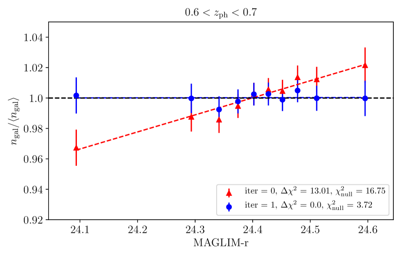
Figure 6: Example of a 1D relation from our set of fiducial SP maps, before (red triangles) and after (blue dots) being corrected using the weights obtained with ISD. Dashed lines correspond to the best linear fits in each case.

Bin	SP maps used to correct for with $T_{\rm 1D}=2$
$0.6<z_{\rm ph}<0.7$	MAGLIM-r
$0.7<z_{\rm ph}<0.8$	FWHM-z, GAIA, FWHM-Y
$0.8<z_{\rm ph}<0.9$	GAIA, FWHM-Y, FWHM-r
$0.9<z_{\rm ph}<1.0$	FWHM-z
$1.0<z_{\rm ph}<1.1$	DIVOT_edensity_GAIA, FWHM-z
$1.1<z_{\rm ph}<1.2$	DIVOT_edensity_GAIA, FWHM-z,
	FWHM-Y, MAGLIM-z

Table 5: List of SP maps found to have impact on the Y6 BAO sample at each redshift bin.

V.3 Stellar Fraction Correction

While most observational systematics modulate the observed number density multiplicatively, $n_{\rm gal}(\theta)\rightarrow(1+f(\theta))n_{\rm gal}(\theta)$, residual stellar contamination represents an additional and undesired population in our sample, which contributes additively as $n_{\rm gal}(\theta)\rightarrow n_{\rm gal}(\theta)+n_{\rm star}(\theta)$. Defining the overdensity of each population as $\delta_{X}=n_{X}/\bar{n}_{X}-1$, with $X\in\{{\rm gal},{\rm star}\}$, and $f_{\rm star}=\bar{n}_{\rm star}/(\bar{n}_{\rm gal}+\bar{n}_{\rm star})$,

$$\delta_{\rm obs}=\delta_{\rm gal}+f_{\rm star}(\delta_{\rm star}-\delta_{\rm gal}).$$ (23)

In the limit where the density of stars is smoothly varying relative to the density of galaxies, we can approximate $\delta_{\rm star}\sim 0$. Therefore, the net effect is a suppression of galaxy fluctuations by an overall factor,

$$\delta_{\rm obs}\approx\delta_{\rm gal}(1-f_{\rm star}).$$ (24)

This is equivalent to modifying the integral constraint, and is an effect that is perfectly degenerate with linear galaxy bias, as noted in [72]. The contribution from spatially varying contamination that is neglected in Equation 24 is captured to first order by the standard treatment described in subsection V.2 when computing galaxy weights through the inclusion of a stellar density map from Gaia, and so we only need to estimate an overall average $f_{\rm star}$ (see also [73], wherein a similar approach is applied with HSC data).

We estimate stellar contamination through the same procedure used for the Y6 lens galaxy samples [65], and refer the reader there for more detail. Briefly, we match our BAO sample to the public DECaLS DR9 catalog [74], which includes forced unWISE photometry [75]. Because of a peak in stellar SEDs at $\sim 1.6\mu$m, galaxies that have been redshifted appear relatively brighter in the unWISE W1 band, making stars and galaxies appear in different parts of the $(r-z,z-W1)$ color-space. For each redshift bin, we plot the density of matched objects in the $(r-z,z-W1)$ color-space and define a piecewise linear relation that traces the trough between the peaks that are NIR-bright (galaxies) and those that are NIR-faint (stars).

We compute $f_{\rm star}$ as the fraction of all objects on the NIR-faint side of the piecewise separation in each bin, finding

$$f_{\rm star}=[2.3\%,\ 2.7\%,\ 3.3\%,\ 2.3\%,\ 0.8\%,\ 0.7\%],$$ (25)

with $1\sigma$ uncertainty of roughly 0.15%.

The resultant clustering measurements, i.e., $w(\theta)$, $C_{\ell}$ and $\xi_{p}(s_{\perp})$, are corrected by a factor of $(1-f_{\rm star})^{-2}$ to account for this, though for template-based BAO measurements, such as the one we run in [37], this effect is negligible due to its degeneracy with other nuisance parameters.

VI Unblinding the Clustering Measurements

As we already mentioned, in [37] we perform the measurement of the BAO distance scale using the clustering measurements from the sample optimized in this paper. The analysis is performed blind, which effectively means that the results of our measurements cannot be reported and that the clustering measurements on the data cannot be plotted until a battery of robustness tests has been passed (these tests are described in detail in [37]). This blinding criteria is similar to the one used during the Y3 BAO analysis, see [26]. By the time we included this section in the paper, these tests had already been passed, and we were ready to unblind the clustering measurements of our sample.

In Figure 7 we show the angular correlation functions ($w(\theta)$), the angular power spectra ($C_{\ell}$) and the projected correlation function ($\xi_{p}(s_{\perp})$) for the different redshift bins. These are the three different estimators that we use to measure the BAO feature in [37]. We include the cases of not correcting and correcting for the observational systematics (blue and orange points with error-bars, respectively), as described in subsection V.2. The errors were computed from the diagonals of the fiducial CosmoLike covariance matrix (or Gaussian covariance for $\xi_{p}$) used to run the BAO fits in [37]. The blue band corresponds to the 1$\sigma$ region computed from the 1952 COLA simulations generated for our analysis, i.e., the average clustering signal of the COLA mocks $\pm$ the square root of the diagonal of their covariance, see [37] for further details on the simulations. The effect of the observational systematics is an increase in the amplitude of the clustering. This increase in the amplitude becomes more important with redshift, being the last two redshift bins the ones with the highest contamination.

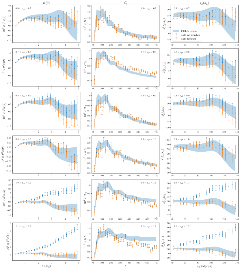
Figure 7: Clustering measurements for the 6 tomographic redshift bins of our BAO sample. The column on the left shows the angular correlation function ($w(\theta)$), the middle one shows the angular power spectra ($C_{\ell}$) and the one on the right shows the projected correlation function ($\xi_{p}(s_{\perp})$). We show the results for the cases of not correcting and correcting the systematics (blue and orange points with error-bars, respectively). The errors were computed from the diagonals of the fiducial CosmoLike covariance matrix (or Gaussian covariance for $\xi_{p}$) used to run the BAO fits in [37]. The blue band corresponds to the 1$\sigma$ region coming from the 1952 COLA simulations generated for our analysis (i.e., the average clustering signal of the COLA mocks $\pm$ the square root of the diagonal of their covariance), see [37] for further details.

VII Conclusions

In this paper we have presented the data used in the DES Y6 analysis for cosmological constraints from the measurement of the BAO distance scale. The sample selection has been optimized with respect to the one used in the Y1 and Y3 analyses: the optimal flux selection is $17.5<i<19.64+2.894z_{\rm ph}$, being $17.5<i<19+3z_{\rm ph}$ the one used for the Y1/Y3. Compared to the Y3 sample, the Y6 optimal sample has one more redshift bin, $1.1<z_{\rm ph}<1.2$, increasing its effective redshift from 0.835 to 0.867. The sample covers 4,273.42 deg² to a depth of $i<22.5$, a very similar area to that of the Y3, which was 4,108.57 deg². It contains 15,937,556 galaxies, compared to the 7 million galaxies of the Y3 sample. This large increase in the number of galaxies with respect to the Y3 is due to the optimized $i$-magnitude cut. We forecast an increase in the precision of the measurement of the BAO scale of around $25\%$ with respect to the Y3 result using our Y6 optimal sample.

We have calibrated the photometric redshift distributions using VIPERS, a spectroscopic sample which has an overlapping area of 16.3 deg² with the DES footprint and which is complete within our optimal sample selection. This allowed us to use the distributions of VIPERS Z_SPEC as the true redshift distributions of our sample. We also used WZ estimations of the redshift distributions to compare to those of Z_SPEC, and found a very good agreement between them. Because of the noisy nature of both Z_SPEC and WZ, and because of DNF giving wider redshift distributions compared to these two, the redshift distributions used for the fiducial analysis on the data are a combination of DNF results, Z_SPEC and WZ: DNF PDF shifted and stretched to match the properties of WZ in the first 4 bins and those of VIPERS Z_SPEC in the last 2.

Systematics have been mitigated using the ISD algorithm, which was also the fiducial in the Y3 analysis [69]. The residual stellar contamination, which contributes additively to the number density of our galaxy sample, has been corrected with a novel technique, which is further described in [65]. We have found a fraction of stellar contamination from 0.7% to 3.3% in the final BAO sample, depending on the redshift bin. This is corrected at the level of the clustering measurement, either $w(\theta)$, $C_{\ell}$ or $\xi_{p}(s_{\perp})$, multiplying by $(1-f_{\rm star})^{-2}$. As a final result, we included the unblinded clustering measurements of our data ($w(\theta)$, $C_{\ell}$ and $\xi_{p}(s_{\perp})$), correcting and not correcting for the observational systematics. The measurement of the BAO scale using these clustering measurements and its cosmological implications are described in [37].

Appendix A Redshift-Related Quantities

It is worth defining several photo-$z$-dependent quantities that we use throughout this paper:

• $\langle z\rangle$. We define it as the mean photometric redshift of a given redshift bin weighted with the redshift distribution, $n(z)$, of that same redshift bin,

  $$\langle z\rangle=\int dz\hskip 1.42271ptzn(z).$$ (26)

• $W_{68}$. We define it as the width in redshift that encloses 68% of the integral of the redshift distribution, i.e., it is given by

  $$W_{68}=\frac{b-a}{2}$$ (27)

  such that

  $$\int_{0}^{a}dz\hskip 1.42271ptn(z)=\int_{b}^{\infty}dz\hskip 1.42271ptn(z)=0.1585.$$ (28)

• $\sigma_{68}$ ($=\Sigma_{z}$). We define it as the size of the region that encloses 68% of the distribution of

  $$\frac{\textsc{DNF\_Z}-\textsc{DNF\_ZN}}{1+\textsc{DNF\_ZN}}.$$ (29)

  Unlike the previous two, $\sigma_{68}$ is a DNF-related quantity, and cannot be computed for all our alternative estimations of the redshift distributions.

Appendix B Calibration of Photometric Redshifts Using VIPERS

Our goal here is to explicitly calibrate our photo-$z$ using VIPERS. In order to do so, we compare the redshift distributions of the BAO sample, computed with DNF_ZN, with those of VIPERS, also computed with DNF_ZN (we actually use the sub-sample of VIPERS matched to the BAO sample). If these two are statistically compatible, we can use the distributions of Z_SPEC as our true redshift distributions, since VIPERS is representative of our full sample. Given that VIPERS is complete and is defined within the selection cuts of our samples, this holds true, but here we explicitly demonstrate it.

The first step to validate the photo-$z$ is to select those galaxies from VIPERS that also belong to the BAO sample. Hereafter, we refer to this sample as VIPERS for simplicity. After matching with the BAO sample, we end up with 11,202 VIPERS galaxies, i.e., VIPERS represents, approximately, a 0.066% of the total number of galaxies in the BAO sample. It is also worth mentioning that, in order to take into account the spectroscopic success ratio of VIPERS, which is encoded in the variable ssr of the VIPERS catalog [47], we must weight each VIPERS galaxy with $1/\textsc{ssr}$.

To quantitatively compare the distributions of DNF_ZN of the BAO sample and VIPERS (both of them shown in Figure 4 as blue histograms and blue points with error-bars, respectively), we calculate the $\chi^{2}$ between them as

$$\chi^{2}=\sum_{i}\frac{\left[n_{\rm BAO}(z_{i})-n_{\rm VIPERS}(z_{i})\right]^{2}}{\Delta n_{\rm VIPERS}(z_{i})^{2}},$$ (30)

where the sum over $i$ means summing over histogram bins, and $\Delta n(z)$ is the shot-noise contribution to the error in the redshift distributions (which is negligible for the BAO sample, because of the large number of galaxies compared to that of VIPERS). In Table 6 we show the reduced $\chi^{2}$ obtained using Equation 30, and also their corresponding p-values, for each redshift bin. All the $\chi^{2}$ and p-values show that both samples are compatible.

Bin	$\chi^{2}$/dof	p-value
$0.6<z_{\rm ph}<0.7$	1.29	0.23
$0.7<z_{\rm ph}<0.8$	0.87	0.57
$0.8<z_{\rm ph}<0.9$	1.08	0.37
$0.9<z_{\rm ph}<1.0$	1.68	0.08
$1.0<z_{\rm ph}<1.1$	1.54	0.12
$1.1<z_{\rm ph}<1.2$	1.07	0.38

Table 6: Reduced $\chi^{2}$ between the redshift distributions of DNF_ZN of the Y6 BAO sample and VIPERS.

Appendix C Calibration of the Redshift Distributions for the PCF

In the projected correlation function (PCF) modeling, we need to utilize fine $\Delta z_{\rm ph}$ bins in order to accurately sample the true redshift distributions [77]. Compared to the Y3 [78], in the Y6 analysis we go to higher redshifts, and that makes this task even more challenging. Rather than using uniform $\Delta z_{\rm ph}$ bins as in the Y3 analysis, we adopt 22 logarithmic bins in the redshift range from 0.6 to 1.2. We calibrate these distributions following the same method as the fiducial 6-bin case discussed in subsection IV.3, i.e., we start with the smooth DNF PDF redshift distributions, and then apply our shift and stretch algorithm to calibrate them using the proxy distribution derived from the WZ technique or the matched VIPERS Z_SPEC one. For the first 17 bins (up to $z_{\rm ph}=1.02$), they are calibrated using the WZ method, whereas for the remaining 5 bins they are calibrated using VIPERS Z_SPEC. This is consistent with what we did in section IV, in which we used WZ for the first 4 redshift bins (i.e., below redshift 1.0) and VIPERS Z_SPEC for the last 2 (i.e., for redshifts between 1.0 and 1.2).

In Figure 8 we compare the original DNF PDF and the shifted and stretched ones. For clarity, we split the bins into three panels, with the upper, middle, and bottom panels corresponding to the bin number modulo 3 being 1, 2, and 0, respectively. We have also plotted the proxy WZ or VIPERS Z_SPEC distributions. The PDF distribution is generally wider than the calibrated one, as expected. The correction also tends to shift the distribution to a slightly lower redshift, and this shift is observed in most of the redshift bins.

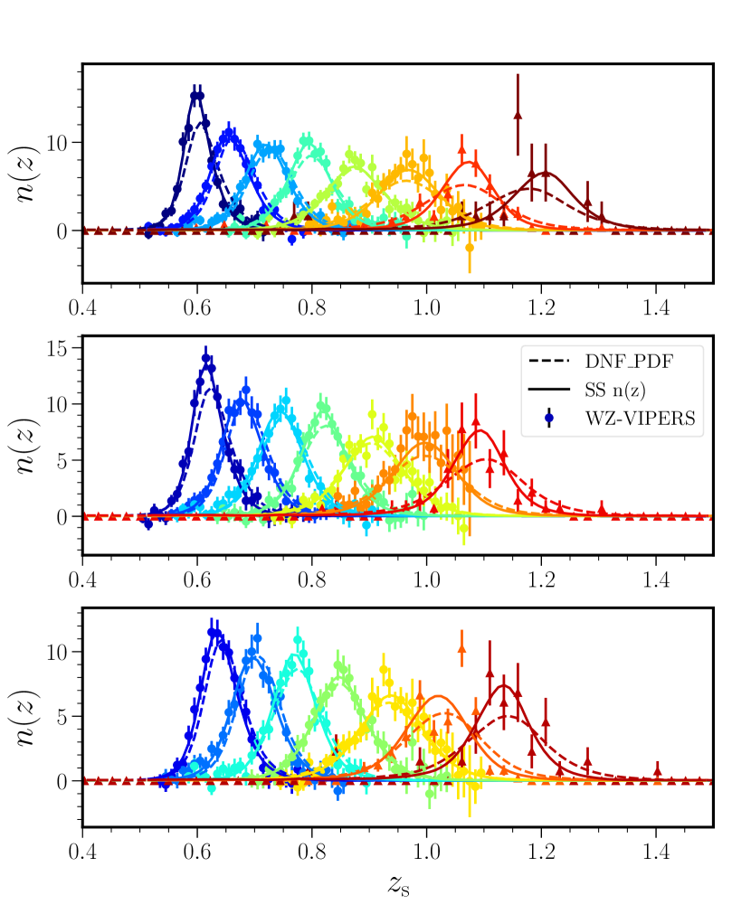
Figure 8: Redshift distributions for the 22 PCF logarithmic bins. The distributions in the upper, middle, and bottom panels correspond to the bin whose bin number modulo 3 is 1, 2, and 0 respectively. The original DNF PDF (dashed) and the shifted and stretched (solid) distributions are compared. The proxy distributions used for the correction are shown in markers: circles for WZ (the first 17 bins) and triangles for matched VIPERS Z_SPEC (the remaining 5 bins).

Appendix D Evolution of the 1D Relations with the Weighting Process

In this appendix we present the evolution of the 1D relation (and, therefore, of the contamination significance) for each of the SP maps we found necessary to correct for, according to ISD. This evolution is illustrated in Figure 9, where for each of the SP maps from Table 5 we show their 1D relation before (in red) and after (in blue) correcting for them at their corresponding iteration. We also show their status at the intermediate iterations (in black).

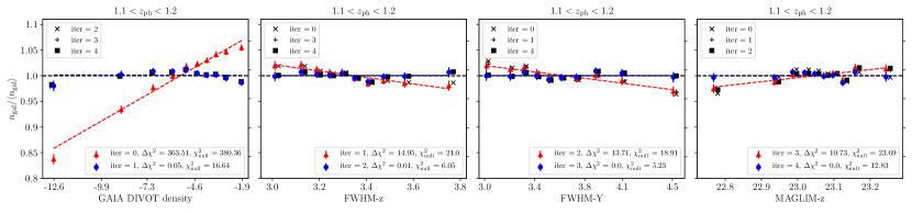
Figure 9: Evolution of the 1D relations as a function of the correcting iteration for each SP map we correct for. Each row corresponds to a redshift bin, starting from the second one (see Figure 6 for first bin). Red triangles show the 1D relation of each of the SP maps from Table 5 before correcting for them, blue dots correspond to their 1D relations right after correcting for them, and the markers in black show their status at the intermediate iterations. Dashed lines represent the best linear fits in each case (from which $\Delta\chi^{2}_{\rm model}$ is computed).

Appendix E Weights Validation Tests

To check the correct functioning of ISD and the weighted obtained with it, we run this method again on the weighted BAO sample using the fiducial set of SP maps presented in subsection V.2. In doing so, we simply evaluate the correct functioning of the method, since by definition all those SP maps should be found to have $S_{\rm 1D}<2$, so no additional corrections should be needed. We find no remaining levels of contamination at $S_{\rm 1D}>2$ coming from any of the fiducial SP maps. After this, we run ISD on the weighted BAO sample, this time using the full list of available SP maps in Y6 (see [43]) and [65]), that is, without limiting the list of contamination templates to the fiducial set presented in subsection V.2. Proceeding this way, we test the validity of our fiducial set of SP maps as a representative set of contamination templates. With this configuration, ISD finds minor levels of additional contamination at some redshift bins in the form of additional (1 to 3) SP maps to be corrected for. However, these numbers are compatible with statistical fluctuations around a strict significance threshold and, given the negligible impact of the weights on the BAO peak, we decide not to incorporate those maps in the final set of corrections. Lastly, we test the assumption of linearity for the corrections by comparing the distribution of $\chi^{2}_{\rm null}$ measured on the weighted BAO sample for all SP maps with a theoretical $\chi^{2}$ distribution with $N_{\rm dof}=10$ (the number of bins used for the 1D relations). Deviations from linearity of the 1D relations and, therefore, of the corresponding (linear) corrections should appear as deviations from a $\chi^{2}$ behaviour of $\chi^{2}_{\rm null}$. The results of this test are depicted in Figure 10. We conclude that the systematic corrections provided by ISD show no significant deviations from linearity. At the forth and sixth redshift bins we observe two outlier values of $\chi^{2}_{\rm null}$, but checking the 1D relations of those two SP maps we find them still compatible with linearity ($\chi^{2}_{\rm model}=11.6$ and $14.1$ with $N_{\rm dof}=8$). Their slightly outlier values are explained by mild levels of residual contamination not higher than $\sim 4\%$ at the 1D level, which ISD does not flagged as significant enough.

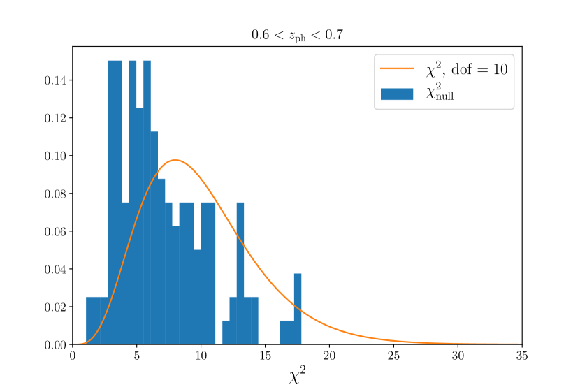
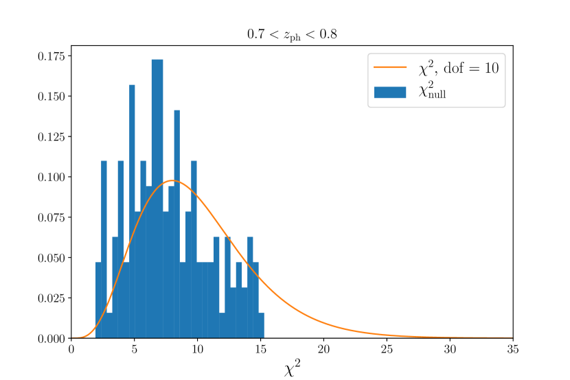
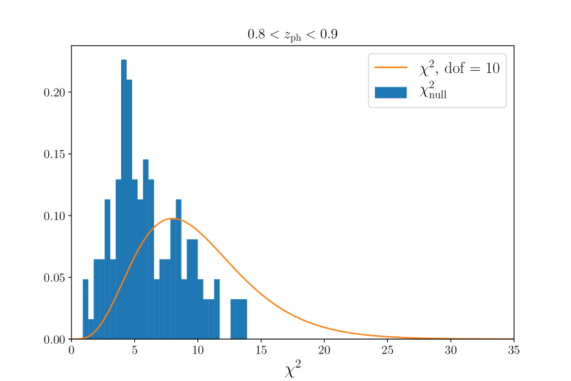
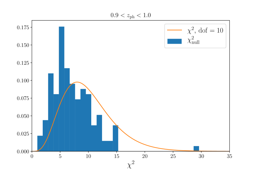
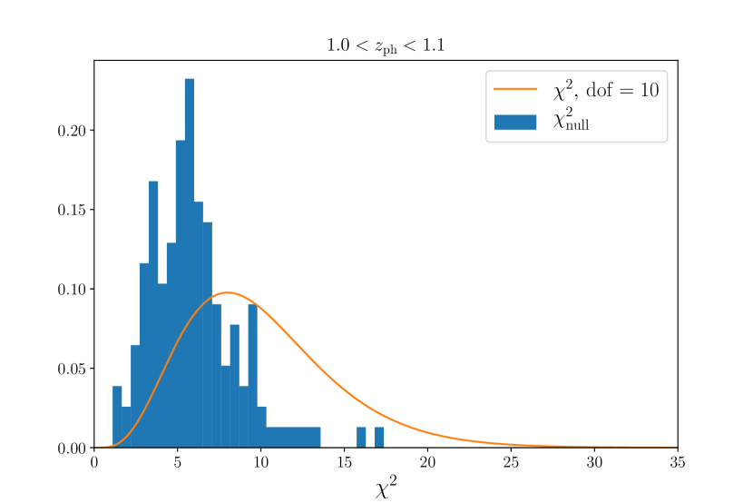
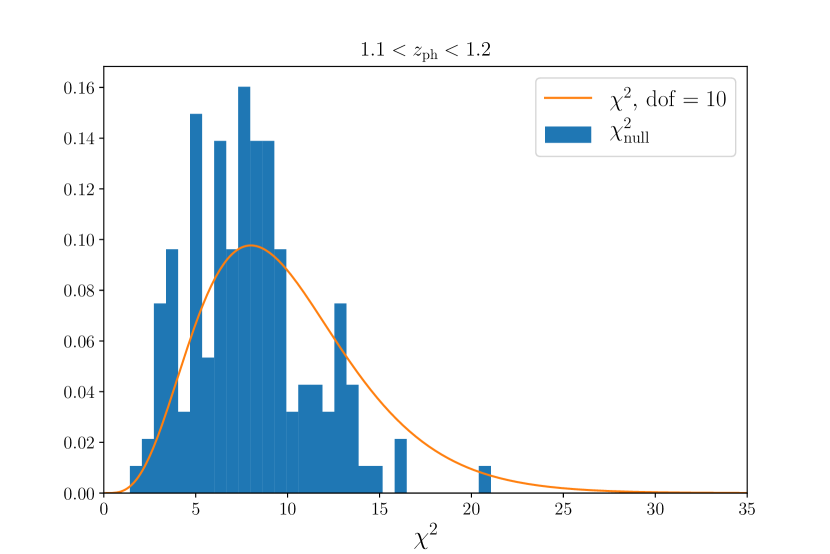
Figure 10: Distribution of $\chi^{2}_{\rm null}$ computed on the weighted Y6 BAO sample for all available SP maps. The solid orange line showcases a theoretical $\chi^{2}$ distribution with $N_{\rm dof}=10$. We find no significant deviations of $\chi^{2}_{\rm null}$ from the theoretical distribution, meaning that the linear assumption for the systematic correction is valid to the extent, i.e., significance threshold, that we consider.

References

- Peebles and Yu [1970] P. J. E. Peebles and J. T. Yu, Astrophys. J. 162, 815 (1970).
- Sunyaev and Zeldovich [1970] R. A. Sunyaev and Y. B. Zeldovich, Ap&SS 7, 3 (1970).
- Bond and Efstathiou [1984] J. R. Bond and G. Efstathiou, ApJ 285, L45 (1984).
- Bond and Efstathiou [1987] J. R. Bond and G. Efstathiou, MNRAS 226, 655 (1987).
- Eisenstein et al. [2005] D. J. Eisenstein et al., Astrophys. J. 633, 560 (2005), arXiv:astro-ph/0501171 [astro-ph] .
- Cole et al. [2005] S. Cole et al., MNRAS 362, 505 (2005), arXiv:astro-ph/0501174 [astro-ph] .
- Percival et al. [2007] W. J. Percival et al., MNRAS 381, 1053 (2007), arXiv:0705.3323 [astro-ph] .
- Gaztañaga et al. [2009] E. Gaztañaga, A. Cabré, and L. Hui, MNRAS 399, 1663 (2009), arXiv:0807.3551 [astro-ph] .
- Percival et al. [2010] W. J. Percival et al., MNRAS 401, 2148 (2010), arXiv:0907.1660 [astro-ph.CO] .
- Beutler et al. [2011] F. Beutler et al., MNRAS 416, 3017 (2011), arXiv:1106.3366 [astro-ph.CO] .
- Blake et al. [2011] C. Blake et al., MNRAS 415, 2892 (2011), arXiv:1105.2862 [astro-ph.CO] .
- Ross et al. [2015] A. J. Ross et al., MNRAS 449, 835 (2015), arXiv:1409.3242 [astro-ph.CO] .
- Alam et al. [2017] S. Alam et al., MNRAS 470, 2617 (2017), arXiv:1607.03155 [astro-ph.CO] .
- Bautista et al. [2021] J. E. Bautista et al., Monthly Notices of the Royal Astronomical Society 500, 736 (2021).
- Gil-Marín et al. [2020] H. Gil-Marín et al., Monthly Notices of the Royal Astronomical Society 498, 2492 (2020).
- De Mattia et al. [2021] A. De Mattia et al., Monthly Notices of the Royal Astronomical Society 501, 5616 (2021).
- Hou et al. [2021] J. Hou et al., Monthly Notices of the Royal Astronomical Society 500, 1201 (2021).
- Neveux et al. [2020] R. Neveux et al., Monthly Notices of the Royal Astronomical Society 499, 210 (2020).
- Alam et al. [2021] S. Alam et al., Physical Review D 103, 083533 (2021).
- Padmanabhan et al. [2007] N. Padmanabhan et al., MNRAS 378, 852 (2007), arXiv:astro-ph/0605302 [astro-ph] .
- Estrada et al. [2009] J. Estrada et al., Astrophys. J. 692, 265 (2009), arXiv:0801.3485 [astro-ph] .
- Hütsi [2010] G. Hütsi, MNRAS 401, 2477 (2010), arXiv:0910.0492 [astro-ph.CO] .
- Crocce et al. [2011] M. Crocce et al., MNRAS 417, 2577 (2011), arXiv:1104.5236 [astro-ph.CO] .
- Carnero et al. [2012] A. Carnero et al., MNRAS 419, 1689 (2012), arXiv:1104.5426 [astro-ph.CO] .
- collaboration [2019] T. D. E. S. collaboration, MNRAS 483, 4866 (2019), arXiv:1712.06209 [astro-ph.CO] .
- collaboration [2022a] T. D. E. S. collaboration, Phys. Rev. D 105, 043512 (2022a).
- Ata et al. [2018] M. Ata et al., MNRAS 473, 4773 (2018), arXiv:1705.06373 [astro-ph.CO] .
- Bautista et al. [2017] J. E. Bautista et al., A&A 603, A12 (2017), arXiv:1702.00176 [astro-ph.CO] .
- Des Bourboux et al. [2020] H. D. M. Des Bourboux et al., The Astrophysical Journal 901, 153 (2020).
- Flaugher [2005] B. Flaugher, International Journal of Modern Physics A 20, 3121 (2005).
- The Dark Energy Survey collaboration [2016] The Dark Energy Survey collaboration, MNRAS 460, 1270 (2016), arXiv:1601.00329 [astro-ph.CO] .
- Eisenstein et al. [2001] D. J. Eisenstein et al., AJ 122, 2267 (2001), arXiv:astro-ph/0108153 [astro-ph] .
- Vakili et al. [2019] M. Vakili et al., MNRAS 487, 3715 (2019), arXiv:1811.02518 [astro-ph.CO] .
- Crocce et al. [2019] M. Crocce et al., Monthly Notices of the Royal Astronomical Society 482, 2807 (2019), arXiv:1712.06211 [astro-ph.CO] .
- Zhou et al. [2020] R. Zhou et al., Research Notes of the American Astronomical Society 4, 181 (2020), arXiv:2010.11282 [astro-ph.CO] .
- De Vicente et al. [2016] J. De Vicente, E. Sánchez, and I. Sevilla-Noarbe, Monthly Notices of the Royal Astronomical Society 459, 3078 (2016).
- The Dark Energy Survey collaboration [2024] The Dark Energy Survey collaboration, to be submitted to PRD (2024).
- Li et al. [2016] T. S. Li, D. L. DePoy, J. L. Marshall, D. Tucker, R. Kessler, J. Annis, et al., AJ 151, 157 (2016), arXiv:1601.00117 [astro-ph.IM] .
- Burke et al. [2018] D. L. Burke et al., AJ 155, 41 (2018), arXiv:1706.01542 [astro-ph.IM] .
- Flaugher et al. [2015] B. Flaugher, H. T. Diehl, K. Honscheid, et al., AJ 150, 150 (2015), arXiv:1504.02900 [astro-ph.IM] .
- Morganson et al. [2018] E. Morganson et al., Publications of the Astronomical Society of the Pacific 130, 074501 (2018).
- Abbott et al. [2021] T. M. C. Abbott et al., ApJS 255, 20 (2021), arXiv:2101.05765 [astro-ph.IM] .
- Bechtol et al. [2024] K. Bechtol et al., to be submitted to ApJS (2024).
- The Dark Energy Survey collaboration [2022] The Dark Energy Survey collaboration, MNRAS 509, 3547 (2022), arXiv:2012.12824 [astro-ph.CO] .
- Rosell et al. [2021a] A. C. Rosell et al., Monthly Notices of the Royal Astronomical Society 509, 778 (2021a), https://academic.oup.com/mnras/article-pdf/509/1/778/41118809/stab2995.pdf .
- Gschwend et al. [2018] J. Gschwend et al., Astronomy and Computing 25, 58 (2018), arXiv:1708.05643 [astro-ph.GA] .
- Scodeggio et al. [2018] M. Scodeggio et al., Astronomy & Astrophysics 609, A84 (2018).
- Seo and Eisenstein [2007] H.-J. Seo and D. J. Eisenstein, The Astrophysical Journal 665, 14 (2007).
- Tegmark [1997] M. Tegmark, Physical Review Letters 79, 3806 (1997).
- Rosell et al. [2021b] A. C. Rosell et al., Monthly Notices of the Royal Astronomical Society 509, 778 (2021b), https://academic.oup.com/mnras/article-pdf/509/1/778/41118809/stab2995.pdf .
- Newman [2008] J. A. Newman, Astrophys. J. 684, 88-101 (2008), arXiv:0805.1409 .
- Matthews and Newman [2010] D. J. Matthews and J. A. Newman, Astrophys. J. 721, 456 (2010), arXiv:1003.0687 [astro-ph.CO] .
- McQuinn and White [2013] M. McQuinn and M. White, MNRAS 433, 2857 (2013), arXiv:1302.0857 [astro-ph.CO] .
- Ménard et al. [2013] B. Ménard et al., arXiv e-prints , arXiv:1303.4722 (2013), arXiv:1303.4722 [astro-ph.CO] .
- Choi et al. [2016] A. Choi et al., MNRAS 463, 3737 (2016), arXiv:1512.03626 [astro-ph.CO] .
- Scottez et al. [2016] V. Scottez et al., MNRAS 462, 1683 (2016), arXiv:1605.05501 [astro-ph.CO] .
- Johnson et al. [2016] A. Johnson et al., Monthly Notices of the Royal Astronomical Society 465, 4118 (2016), https://academic.oup.com/mnras/article-pdf/465/4/4118/10254854/stw3033.pdf .
- Hildebrandt et al. [2021] H. Hildebrandt et al., Astronomy & Astrophysics 647, A124 (2021).
- van den Busch et al. [2020] J. L. van den Busch et al., A&A 642, A200 (2020), arXiv:2007.01846 [astro-ph.CO] .
- Cawthon et al. [2022] R. Cawthon et al., Monthly Notices of the Royal Astronomical Society 513, 5517 (2022).
- Reid et al. [2016] B. Reid et al., Monthly Notices of the Royal Astronomical Society 455, 1553 (2016).
- Ross et al. [2020] A. J. Ross et al., MNRAS 498, 2354 (2020), arXiv:2007.09000 [astro-ph.CO] .
- Raichoor et al. [2021] A. Raichoor et al., Monthly Notices of the Royal Astronomical Society 500, 3254 (2021).
- collaboration [2022b] T. D. E. S. collaboration, Phys. Rev. D 105, 023520 (2022b).
- Weaverdyck et al. [2024] N. Weaverdyck et al., to be submitted to PRD (2024).
- Rodriguez-Monroy et al. [2024] M. Rodriguez-Monroy et al., to be submitted to PRD (2024).
- Schlegel et al. [1998] D. J. Schlegel, D. P. Finkbeiner, and M. Davis, Astrophys. J. 500, 525 (1998), astro-ph/9710327 .
- Gaia Collaboration et al. [2020] Gaia Collaboration et al., arXiv e-prints , arXiv:2012.01533 (2020), arXiv:2012.01533 [astro-ph.GA] .
- Rodríguez-Monroy et al. [2021] M. Rodríguez-Monroy et al., Dark Energy Survey Year 3 Results: Galaxy clustering and systematics treatment for lens galaxy samples (2021), arXiv:2105.13540 [astro-ph.CO] .
- Elvin-Poole et al. [2018] J. Elvin-Poole et al., Phys. Rev. D 98, 042006 (2018), arXiv:1708.01536 [astro-ph.CO] .
- Weaverdyck and Huterer [2021] N. Weaverdyck and D. Huterer, MNRAS 503, 5061 (2021), arXiv:2007.14499 [astro-ph.CO] .
- Krolewski et al. [2020] A. Krolewski et al., Journal of Cosmology and Astroparticle Physics 2020 (05), 047.
- Nicola et al. [2020] A. Nicola et al., Journal of Cosmology and Astroparticle Physics 2020 (03), 044.
- Dey et al. [2019] A. Dey et al., The Astronomical Journal 157, 168 (2019).
- Schlafly et al. [2019] E. F. Schlafly et al., The Astrophysical Journal Supplement Series 240, 30 (2019).
- Zhou et al. [2023] R. Zhou et al., The Astronomical Journal 165, 58 (2023).
- Chan et al. [2022a] K. C. Chan et al., MNRAS 511, 3965 (2022a), arXiv:2110.13332 [astro-ph.CO] .
- Chan et al. [2022b] K. C. Chan et al., Phys. Rev. D 106, 123502 (2022b), arXiv:2210.05057 [astro-ph.CO] .