Flat-band engineering of quasi-one-dimensional systems via supersymmetric transformations

Abstract

We introduce a systematic method to spectrally design quasi-one-dimensional crystal models described by the Dirac equation in the low-energy regime. The method is based on the supersymmetric transformation applied to an initially known pseudo-spin-1/2 model. This allows extending the corresponding susy partner so that the new model describes a pseudo-spin-1 system. The spectral design allows the introduction of a flat-band and discrete energies at will into the new model. The results are illustrated in two examples where the Su-Schriefer-Heeger chain is locally converted into a stub lattice.

1 Introduction

Advances in the experimental techniques make it possible to create artificial materials, either by molecular manipulations [1, 2, 3, 4, 5], photonic lattices [6, 7], or in phononic experiments [8, 9]. They provide unprecedented control over physical properties and effective interactions in the created systems. In particular, it is possible to prepare one-dimensional crystallic chains with diverse structure, e.g. Su-Schriefer-Heeger, stub, diamond (rhombic), Creutz, or fishbone lattices [7, 10, 11]. These systems attract attention due to their simple structure yet rich properties, e.g. existence of topological states [12, 13, 14, 15], bulk-edge correspondence [16], Aharonov-Bohm caging [17, 18, 19, 20] or superconductivity [21, 22]. Many of these properties are related to the existence of flat-band in their spectra. The flat-band is associated with vanishing group velocity and macroscopical degeneration of eigenstates. It was observed experimentally in optical lattices [11, 23, 24, 25].

There is both experimental [10] and theoretical effort [26, 27] to provide useful tools and methods for engineering of the flat-band systems. It was proposed via repetition of microarrays [26], via polynomials of tight-binding Hamiltonian [27], via compact localized states classification [28], graph theory [29, 30]. The methods frequently rely on the tight-binding approach. In this article, we will resolve to the Dirac approximation where dynamics is described by Dirac equation with pseudo-spin one. Our approach will be based on supersymmetric quantum mechanics where the existence of flat-band is granted by construction.

Supersymmetric transformation, equivalent known in this context in the literature as Darboux transformation, is a specific non-unitary mapping between evolution equations of two quantum systems. It can be used for the construction of the new solvable models in the way that the potential term of the initial system gets deformed, yet, the knowledge of the solutions is preserved. It was very popular in non-relativistic quantum mechanics [31]. In the last years, it was utilized in the construction of solvable models described by one- or two-dimensional Dirac equation. Supersymmetric transformation for low-dimensional Dirac operators was discussed in [32, 33], and employed in a series of works, see e.g. [34, 35, 36, 37, 38, 39, 40, 41, 42, 43, 44]. Most of them focus on the analysis of pseudo-spin$-1/2$ quantum systems. The supersymmetric transformation was recently applied in the context of pseudo-spin-1 flat-band systems in [45].

The Su-Schriefer-Heeger (SSH) model is a one-dimensional chain of dimerized atoms. The model was used originally for analysis of solitonic effects in macromolecules [46, 47]. It also possesses non-trivial topological properties [48]. The low-energy approximation of its tight-binding Hamiltonian corresponds to the one-dimensional Dirac operator [47]. Solitonic states emerge in SSH ladders on domain walls, where the dimerization of atoms gets inverted. Domain walls on SSH-type chains of coupled dimers were experimentally realized on chlorine vacancies in the c(2$\times$2) adsorption layer on Cu(100) in [13]. The existence of topological domain wall states was discussed in [49, 50], whereas the supersymmetric transformation has been applied to induce a topological gapped state in the SSH chain [51, 52]. Furthermore, the transmission properties of pseudo-spin-1 Dirac equations described through decorated, “bearded,” SSH chains have been discussed [53].

In this article, the supersymmetric transformation is exploited to connect known pseudo-spin-$1/2$ quantum models with new unknown pseudo-spin-1 models. Particularly, the transformation allows tuning the emerging flat band of the new model while adding new bound state energies, assuming that the proper boundary conditions are met. To this end, a pseudo-spin-1/2 model is trivially extended into a pseudo-spin-1 system by adding an isolated coupling term, such that the dispersion relations are kept invariant. This allows matching the supersymmetric transformation with a new and non-trivially extended pseudo-spin-1 system, where the added coupled term is no longer isolated and now describes an interaction with the rest of the elements in the system. Particularly, a massive free particle graphene-like system is used as the initial model in the transformation, leading to explicit models that behave asymptotically as an SSH chain with altered dimerization patterns resembling the domain wall. Such an SSH chain gets locally decorated by additional atoms, forming a stub lattice in the localized region. This allows for a systematic mechanism to spectrally manufacture pseudo-spin-1 models based on relatively simple pseudo-spin-$1/2$ models.

The manuscript is structured as follows. Section 2 summarizes the periodic structure and dispersion bands of the generalized stub lattice, where the special case where a flat-band emerges is considered. In Section 3, the general framework of the Darboux transform (susy transform) for arbitrary pseudo-spin systems is briefly introduced. Here, the transformation is implemented for an extended pseudo-spin-1/2 so that the susy partner renders a non-trivial pseudo-spin-1 model. Applications of the latter are further exemplified in Section 4 and Section 5, where explicit cases of quasi-one-dimensional pseudo-spin-1 systems are derived and discussed. Further discussions and future perspectives for future applications of the present results are detailed in Section 6.

2 Generalized stub lattice

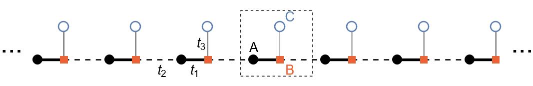
(a)

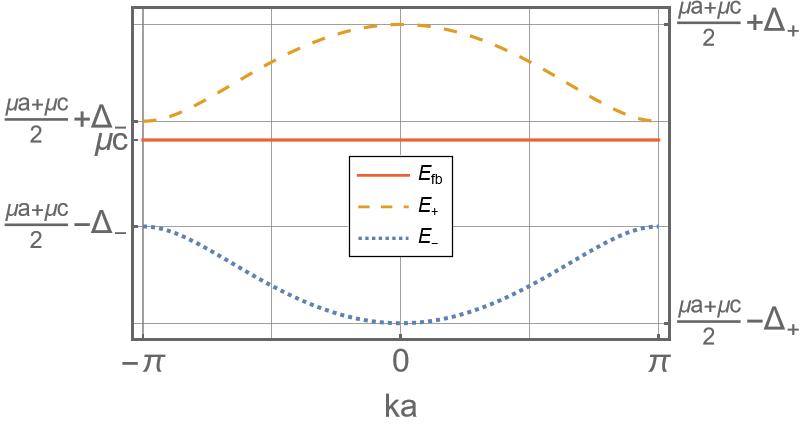
(b)

Figure 1: (a) Sketch of the periodic pseudo-one-dimensional stub lattice with three atoms $A$, $B$, and $C$ per unitary cell (dashed rectangle). The hopping parameters are denoted by $t_{1}$, $t_{2}$, and $t_{3}$. (b) Dispersion relations (5) in terms of the hopping parameters and the on-site interactions $\mu_{A}$ and $\mu_{B}=\mu_{C}$, where $\Delta_{\pm}=\sqrt{(t_{1}\pm t_{2})^{2}+t_{3}^{2}+\frac{(\mu_{A}-\mu_{C})^{2}}{4}}$.

Let us consider the tight-biding model of generalized stub lattice where the hopping amplitudes are considered real but general otherwise. The model here is such that it converges to the SSH lattice or stub lattice for specific choices of the hopping parameters. The tight-binding Hamiltonian $H_{gs}$ of a generalized stub lattice (see Fig.1a) is

$$H_{gs}=\sum_{n}(t_{1}A_{n}^{\dagger}B_{n}+t_{2}A_{n}^{\dagger}B_{n-1}+t_{3}A_{n}^{\dagger}C_{n}+\mu_{A}A_{n}^{\dagger}A_{n}+\mu_{B}B_{n}^{\dagger}B_{n}+\mu_{C}C_{n}^{\dagger}C_{n})+h.c.$$ (1)

where $A_{n}^{\dagger}$, $B_{n}^{\dagger}$, and $C_{n}^{\dagger}$ are fermionic creation operators for electrons on site $A_{n}$ $B_{n}$ or $C_{n}$. The quantities $t_{1}$, $t_{2}$ and $t_{3}$ are the real hopping amplitudes, $\mu_{A,B,C}$ correspond to real on-site energies. The index $n$ runs over all elementary cells. The primitive translation vector is $(a,0)$. Therefore, the first Brillouin zone is $k\in\left[0,\frac{2\pi}{a}\right]$. Fourier transform of $H$ provides us with the following operator

$$H_{gs}(k)=\begin{pmatrix}\mu_{A}&t_{1}+t_{2}e^{-ika}&t_{3}\\ t_{1}+t_{2}e^{ika}&\mu_{B}&0\\ t_{3}&0&\mu_{C}\end{pmatrix}.$$ (2)

The secular equation $\det(H_{gs}(k)-\lambda)=0$ reads as

$$(\lambda-\mu_{B})t_{3}^{2}+(\lambda-\mu_{C})(t_{1}^{2}+t_{2}^{2}-(\lambda-\mu_{A})(\lambda-\mu_{B})+2t_{1}t_{2}\cos ak)=0.$$ (3)

Although the latter can be solved for any $\lambda$ (for more details, see [54]), we are interested in the configuration where the flat-band is present. Indeed, this occurs for

$$\mu_{B}=\mu_{C},$$ (4)

which, henceforth, is the case under consideration. This leads to the dispersion relations of the form

$$E_{fb}=\mu_{C},\quad E_{\pm}=\frac{\mu_{A}+\mu_{C}}{2}\pm\sqrt{t_{1}^{2}+t_{2}^{2}+t_{3}^{2}+\frac{(\mu_{A}-\mu_{C})^{2}}{4}+2t_{1}t_{2}\cos ka}.$$ (5)

From the latter, it is worth remarking that dispersion bands never touch; i.e., the band structure is always gapped. This is a stark difference with respect to other flat band systems such as the two-dimensional Lieb lattice [54], where vanishing next-nearest neighbors close the band gap. Furthermore, the trimer SSH model [16] does not hold a flat band in its spectrum.

Our model can be reduced to a couple of special cases when the parameters are fixed correspondingly. That is, for $t_{3}=0$, the $C$ atoms are effectively isolated from the linear chain formed by $A$ and $B$ atoms. The $C$ atoms host the flat-band states with energy $\mu_{C}$. These states are strongly localized at the $C$ atoms as there is no interaction with other atoms. In turn, for $t_{1}\neq t_{2}$, the linear chain of $A-B$ atoms coincides with an infinite $SSH$ model. The case $t_{1}=t_{2}=t_{3}$ reproduces the stub lattice. The band structure of the system is illustrated in Fig. 1b.

The energy band $E_{+}$ ($E_{-}$) has its minimum (maximum) at $K=\frac{\pi}{a}$. Expanding the Hamiltonian (2) for $k=K+\delta k$ up to the first order in $\delta k$, we get

$$H_{gs}(K+\delta k)\sim\begin{pmatrix}\mu_{A}&t_{1}-t_{2}+iat_{2}\delta k&t_{3}\\ t_{1}-t_{2}-iat_{2}\delta k&\mu_{C}&0\\ t_{3}&0&\mu_{C}\end{pmatrix}.$$ (6)

It is a Dirac-type operator for three-component wave functions. We prefer to make an additional transformation defined as $(\psi_{1},\psi_{2},\psi_{3})\rightarrow(\psi_{1},i\,\psi_{2},i\,\psi_{3})$. The resulting operator in coordinate representation reads as

$$h_{gs}(k)=\begin{pmatrix}\mu_{A}&-i(t_{1}-t_{2})-iat_{2}\partial_{x}&-i\,t_{3}\\ i(t_{1}-t_{2})-iat_{2}\partial_{x}&\mu_{C}&0\\ i\,t_{3}&0&\mu_{C}\end{pmatrix}.$$ (7)

In the next section, the method will be presented where the systems described by (7) with possibly inhomogeneous hopping $t_{1}$ and $t_{3}$ can be constructed. Our approach will be based on supersymmetric transformation that will provide the coupling between the two linear chains of atoms.

3 Coupling via Darboux transformation

Let us start the section with a brief review of Darboux transformation for Dirac-type operator $H=-i\gamma\partial_{x}+V$, where $\gamma$ and $V$ can be generic $N\times N$ matrices. The Darboux transformation for $N=2$ was discussed in [32], while the general case was considered in [33]. Darboux transformation relates the initially known stationary equation $(H-\epsilon)\Psi=0$ with the new unknown equation $(\tilde{H}-\epsilon)\tilde{\Psi}=0$, where $\tilde{H}=-i\gamma\partial_{x}+\tilde{V}$ is also a Dirac-type operator with an altered potential term. Furthermore, the Darboux transformation maps the solutions of the first equation into the solutions of the second equation. It is represented by a differential operator, i.e. it is not unitary and it is not a one-to-one mapping.

The transformation is based on $N$ eigenstates $\Psi_{a}$, $a=1,2,\dots,N$, of $H$, $(H-\lambda_{a})\Psi_{a}=0$. The eigenstates are used to compose an $N\times N$ matrix $U=(\Psi_{1}\,\Psi_{2}\,\dots\,\Psi_{N})$. There holds

$$HU=U\Lambda,\quad\Lambda=\mbox{diag}\{\lambda_{1},\lambda_{2},\dots,\lambda_{N}\},$$ (8)

so that we can define the new Dirac-type operator

$$\tilde{H}=-i\gamma\partial_{x}+\tilde{V}=-i\gamma\partial_{x}+V-\delta V,\quad\delta V=i[\gamma,U_{x}U^{-1}].$$ (9)

The latter is related with $H$ through the intertwining relation $LH=\tilde{H}L$, where $L$ is the first-order differential operator

$$L=U\partial_{x}U^{-1}.$$ (10)

Here, the operator $L$ effectively maps the eigenstates of $H$ into the eigenstates of $\tilde{H}$, with the exception of the states $\Psi_{a}$, $a=1,\dots,N$ that belong to the kernel of $L$. Indeed, there holds

$$(H-\epsilon)\Psi=0\Longrightarrow(\tilde{H}-\epsilon)\tilde{\Psi}=0,\quad\tilde{\Psi}=L\Psi.$$ (11)

Let us consider a generic, one-dimensional pseudo-spin-$1/2$ Dirac system described by the following stationary equation

$$H_{1/2}\Psi=\begin{pmatrix}m(x)+v(x)&-i\partial_{x}-iA(x)\\ -i\partial_{x}+iA(x)&-m(x)+v(x)\end{pmatrix}\begin{pmatrix}i\,\psi\\ \phi\end{pmatrix}=\epsilon\begin{pmatrix}i\,\psi\\ \phi\end{pmatrix},$$ (12)

where $m(x)$, $v(x)$ and $A(x)$ are real functions so that $H_{1/2}$ is hermitian. We assume that it is possible to find formal solutions of the equation for any real $\epsilon$.

We trivially extend $H_{1/2}$ by an additional degree of freedom. The new operator will have the following form

$$H_{1}=\begin{pmatrix}m(x)+v(x)&-i\partial_{x}-iA(x)&0\\ -i\partial_{x}+iA(x)&-m(x)+v(x)&0\\ 0&0&\lambda\end{pmatrix}.$$ (13)

It represents the system where two subsystems coexist without any mutual interaction. In one of them, dynamics is driven by $H_{1/2}$ while in the second one, dynamics is frozen as the energy operator is constant.

It is straighforward to find the eigenvectors of the extended operator $H_{1}$ from the eigenvectors of $H_{1/2}$. We shall use them to perform the supersymmetric (susy) transformation of $H_{1}$. In order to do so, we fix the matrix $U$, see (8), in the following manner

$$U=\begin{pmatrix}i\psi_{0}&i\psi_{1}&i\psi_{2}\\ \phi_{0}&\phi_{1}&\phi_{2}\\ 0&\xi_{1}&\xi_{2}\end{pmatrix},\quad H_{1}U=U\begin{pmatrix}\epsilon&0&0\\ 0&\lambda&0\\ 0&0&\lambda\end{pmatrix},\quad\epsilon,\lambda\in\mathbb{R}.$$ (14)

The columns of $U$ are formed by the eigenvectors corresponding to the eigenvalues $\epsilon$ or $\lambda$, respectively. The components $\psi_{a}$, $\phi_{a}$, $a=1,2,3$ and $\xi_{1}$ and $\xi_{2}$ can be fixed as real-valued functions. The functions $\xi_{1}$ and $\xi_{2}$ can be arbitrary, but they should not be zero identically as the transformed Hamiltonian with coupled subsystems could not be hermitian in that case, see Appendix.

Having the matrix $U$ fixed, we can construct $L$ and $\tilde{H}$, see (10) and (13), such that the intertwining relation is satisfied. The new potential $\tilde{V}$ is not hermitian in general. Nevertheless, we can enjoy the freedom in the choice of the functions $\xi_{1}$ and $\xi_{2}$ in order to recover hermiticity of $\tilde{V}$ in (13). It is sufficient to fix $\xi_{1}$ in the following manner,

$$\xi_{1}=\xi_{2}\left(c_{1}-\int\frac{(\epsilon-\lambda)(\phi_{2}\psi_{1}-\phi_{1}\psi_{2})}{\xi_{2}^{2}}dx\right)=\xi_{2}\left(c_{1}-\int\frac{(\epsilon-\lambda)\,W_{0}}{\xi_{2}^{2}}dx\right).$$ (15)

Here, $c_{1}$ is a real integration constant. It is worth noticing that $W_{0}\equiv\phi_{2}\psi_{1}-\phi_{1}\psi_{2}$ is a real constant as well. Indeed, the relation $\partial_{x}W_{0}=0$ can be derived when taking into account that $(\psi_{1},\phi_{1})^{t}$ and $(\psi_{2},\phi_{2})^{t}$ are eigenvectors of $H_{1/2}$ corresponding to the same eigenvalue.

The new Hamitonian $\tilde{H}_{1}$ defined in (13) has the following form

$$\tilde{H}_{1}=\begin{pmatrix}0&-i\partial_{x}&0\\ -i\partial_{x}&0&0\\ 0&0&0\end{pmatrix}+\begin{pmatrix}\tilde{v}_{11}+v&-i\,\tilde{v}_{12}&-i\,\tilde{v}_{13}\\ i\tilde{v}_{12}&-\tilde{v}_{11}+v&\tilde{v}_{23}\\ i\,\tilde{v}_{13}&\tilde{v}_{23}&\lambda\end{pmatrix},$$ (16)

where

$$\tilde{v}_{12} =-A+\left(\epsilon-\lambda\right)\frac{\psi_{0}\,(\xi_{2}\psi_{1}-\xi_{1}\psi_{2})-\phi_{0}\,(\xi_{2}\phi_{1}-\xi_{1}\phi_{2})}{\psi_{0}\,(\xi_{2}\phi_{1}-\xi_{1}\phi_{2})-\phi_{0}\,(\xi_{2}\psi_{1}-\xi_{1}\psi_{2})},$$

$$\tilde{v}_{13} =\frac{(\epsilon-\lambda)\,\psi_{0}\,(\phi_{1}\psi_{2}-\phi_{2}\psi_{1})}{\psi_{0}\,(\xi_{2}\phi_{1}-\xi_{1}\phi_{2})-\phi_{0}\,(\xi_{2}\psi_{1}-\xi_{1}\psi_{2})}=\frac{(\epsilon-\lambda)\,\psi_{0}\,W_{0}}{\psi_{0}\,(\xi_{2}\phi_{1}-\xi_{1}\phi_{2})-\phi_{0}\,(\xi_{2}\psi_{1}-\xi_{1}\psi_{2})},$$

$$\tilde{v}_{23} =-\frac{(\epsilon-\lambda)\,\phi_{0}\,(\phi_{1}\psi_{2}-\phi_{2}\psi_{1})}{\psi_{0}\,(\xi_{2}\phi_{1}-\xi_{1}\phi_{2})-\phi_{0}\,(\xi_{2}\psi_{1}-\xi_{1}\psi_{2})},$$

$$\tilde{v}_{11} =-m+(\epsilon-\lambda)\frac{\psi_{0}\,(\xi_{2}\phi_{1}-\xi_{1}\phi_{2})+\phi_{0}\,(\xi_{2}\psi_{1}-\xi_{1}\psi_{2})}{\psi_{0}(\xi_{2}\phi_{1}-\xi_{1}\phi_{2})-\phi_{0}(\xi_{2}\psi_{1}-\xi_{1}\psi_{2})}.$$ (17)

All the nonvanishing components (17) of the potential $\tilde{V}$ share the same denominator $d\equiv\psi_{0}\,(\xi_{2}\phi_{1}-\xi_{1}\phi_{2})-\phi_{0}\,(\xi_{2}\psi_{1}-\xi_{1}\psi_{2})$. It is proportional to $\det U$. Zeros of $d$ can introduce additional singularities into $\tilde{V}$. Such a situation would be undesirable as it would be necessary to introduce additional boundary conditions at the singularities. The additional boundary conditions could compromise the calculation of physically relevant eigenstates of $\tilde{H}_{1}$. Indeed, physical eigenstates of $H_{1}$ could be mapped into the formal eigenstates of $\tilde{H}_{1}$ that would not belong to its domain. Therefore, the elements of the matrix $U$ should be set such that $d$ is a node-less function.

The components $U$ are not independent. Indeed, $\xi_{1}$ is given in terms of $\xi_{2}$, see (15). The functions $\psi_{a}$ can be expressed in terms of $\phi_{a}$, $a=0,1,2$, respectivelly,

$$\psi_{a}=\frac{\phi_{a}^{\prime}+A\phi_{a}}{m+v-\lambda}.$$ (18)

Additionally, $\phi_{1}$ can be expressed via $\phi_{2}$ as they are two linearly independent solutions of

$$-\left[\left(-\partial_{x}+A\right)\frac{1}{m+v-\lambda}\left(\partial_{x}+A\right)\right]\phi_{1,2}+(v-m-\lambda)\phi_{1,2}=0.$$ (19)

Therefore, $d$ is determined by three functions only, $d=d(\phi_{0},\phi_{2},\xi_{2})$ where $\xi_{2}$ is arbitrary in principle. The freedom in its choice can be exploited to keep $\tilde{V}$ free of any additional singularities. We will discuss explicit choice of $\xi_{2}$ in the models that are to be discussed in the next section.

The formulas (17) suggest that a major simplification of the potential $\tilde{V}$ occurs when either $\psi_{0}=0$ or $\phi_{0}=0$. Then there holds $\tilde{v}_{13}=0$ or $\tilde{v}_{23}=0$, respectively. We are interested in the later as $\tilde{V}$ acquires the form of the Dirac operator (7) in this case. It is not possible to set $\phi_{0}=0$ for a generic Hamiltonian $H_{1}$. Nevertheless, it is possible when $H_{1}$ acquires the following specific form

$$H_{1}=\begin{pmatrix}m&-i\partial_{x}-iA(x)&0\\ -i\partial_{x}+iA(x)&-m&0\\ 0&0&\lambda\end{pmatrix},$$ (20)

where $m$ is a real constant. When we fix $\epsilon=m$, then we can find the corresponding eigenstate $(\psi_{0},\phi_{0},0)$ where $\phi_{0}=0$ and $\psi_{0}=\exp\left(\int A(x)dx\right)$. The matrix $U$ then reads as

$$U=\begin{pmatrix}i\exp\left(\int A(x)dx\right)&i\psi_{1}&i\psi_{2}\\ 0&\phi_{1}&\phi_{2}\\ 0&\xi_{1}&\xi_{2}\end{pmatrix},\quad H_{1}U=U\begin{pmatrix}m&0&0\\ 0&\lambda&0\\ 0&0&\lambda\end{pmatrix},\quad\lambda\in\mathbb{R}.$$ (21)

The components of the simplified potential term $\tilde{V}$

$$\tilde{V}=\begin{pmatrix}-\lambda&-i\,\tilde{v}_{12}&-i\,\tilde{v}_{13}\\ i\tilde{v}_{12}&\lambda&0\\ i\,\tilde{v}_{13}&0&\lambda\end{pmatrix}$$ (22)

are as follows

$$\tilde{v}_{12}(x)=-A(x)+\left(m-\lambda\right)\frac{\xi_{2}\psi_{1}-\xi_{1}\psi_{2}}{\xi_{2}\phi_{1}-\xi_{1}\phi_{2}},\quad\tilde{v}_{13}(x)=-\frac{(m-\lambda)\,W_{0}}{\xi_{2}\phi_{1}-\xi_{1}\phi_{2}}.$$ (23)

Taking into account (19), we can write

$$\phi_{1}=\phi_{2}\left(c_{0}-\int\frac{(m-\lambda)W_{0}}{\phi_{2}^{2}}dx\right).$$ (24)

Substituting (15) and (24) into (23), we get

$$\tilde{v}_{12}(x)=-A(x)+\left(m-\lambda\right)\frac{\psi_{2}}{\phi_{2}}+\tilde{v}_{13}\frac{\xi_{2}}{\phi_{2}},$$ (25)

$$\tilde{v}_{13}(x)=-\frac{(m-\lambda)W_{0}}{\xi_{2}\phi_{2}\left(\delta c+W_{0}(m-\lambda)\left(\int\frac{1}{\xi_{2}^{2}}dx+\int\frac{1}{\phi_{2}^{2}}dx\right)\right)},\quad\delta c=c_{0}-c_{1}.$$ (26)

Now, let us compare $\tilde{H}_{1}$ with (7). Comparing the potentials of the two operators,

$$\begin{pmatrix}-\lambda&-i\,\tilde{v}_{12}&-i\,\tilde{v}_{13}\\ i\tilde{v}_{12}&\lambda&0\\ i\,\tilde{v}_{13}&0&\lambda\end{pmatrix}=\begin{pmatrix}\mu_{A}&-i(t_{1}-t_{2})-iat_{2}\partial_{x}&-i\,t_{3}\\ i(t_{1}-t_{2})-iat_{2}\partial_{x}&\mu_{C}&0\\ i\,t_{3}&0&\mu_{C}\end{pmatrix},$$ (27)

we find that they coincide provided that

$$t_{2}=1/a,\quad\mu_{C}\equiv\lambda,\quad\mu_{A}=-\lambda,\quad t_{1}\equiv 1/a+\tilde{v}_{12},\quad t_{3}\equiv\tilde{v}_{13}.$$ (28)

The hopping amplitudes $t_{1}$ and $t_{3}$ in the effective Hamiltonian $\tilde{H}_{1}$ of the quasi-one dimensional chain would be inhomogeneous. In this context, the operator $H_{1}$ described two systems without any mutual interaction. In contrast, the operator $\tilde{H}_{1}$ corresponds to a qualitatively different physical reality; the two subsystems are coupled by $\tilde{v}_{13}$ and $\tilde{v}_{23}$. In the next section, we will apply the presented framework for construction of two explicit models that can be matched with a decorated SSH model. We will discuss two explicit models where the inhomogeneity makes it possible to convert SSH chain to stub lattice locally.

4 Tunable flat-band in the gap

Let us fix the Hamiltonian $H_{1/2}$ in (12) as the energy operator of a massive particle with pseudo-spin-1/2. The trivially extended operator $H_{1}$ then reads as

$$H_{1}=\begin{pmatrix}m&-i\partial_{x}-iA&0\\ -i\partial_{x}+iA&-m&0\\ 0&0&\lambda\end{pmatrix},$$ (29)

where $m$, $A$ and $\lambda$ are real constants. Its eigenvectors can be found for any $\epsilon$. In accordance with the results of the previous section, we fix $\epsilon=m$ and

$$\psi_{0}=e^{Ax},\quad\phi_{0}=0,\quad(H_{1}-m)(i\psi_{0},\phi_{0},0)=0.$$ (30)

As mentioned in (18) and (19), the components $\psi_{1,2}$ and $\phi_{1}$ can be obtained in terms of $\phi_{2}$. We will assume that $|\lambda|\neq|m|$. Then we can write

$$\psi_{1,2}=\frac{\phi_{1,2}^{\prime}+A\phi_{1}}{m-\lambda},\quad\phi_{1}=\phi_{2}\left(\int\frac{W_{0}(m-\lambda)}{\phi_{2}^{2}}+c_{0}\right),$$ (31)

where $c_{0}$ is a real constant. We used the fact that $\phi_{1}$ and $\phi_{2}$ have to solve the same differential equation (19) of the second order. We assume that they are linearly independent, i.e. the Wronskian $W_{0}$ of the two solutions is nonvanishing, $W_{0}\neq 0$.

The functions $\phi_{2}$ and $\xi_{2}$ are to be selected such that the components (17) of $\tilde{V}_{1}$ are free of singularities. We make the following choice,

$$\quad\phi_{2}=\cosh\kappa x,\quad\xi_{2}=-\rho\cosh\kappa x,\quad\kappa=\sqrt{m^{2}+A^{2}-\lambda^{2}},\quad\rho\in\mathbb{R}.$$ (32)

Here we assume that $A$, $m$, and $\lambda$ are fixed such that $\kappa$ is real. The Hamiltonian $\tilde{H}_{1}$ has the following explicit form

$$\tilde{H}_{1}=\begin{pmatrix}0&-i\partial_{x}&0\\ -i\partial_{x}&0&0\\ 0&0&0\end{pmatrix}+\begin{pmatrix}-\lambda&-i\,\tilde{v}_{12}&-i\,\tilde{v}_{13}\\ i\,\tilde{v}_{12}&\lambda&0\\ i\,\tilde{v}_{13}&0&\lambda\end{pmatrix},$$ (33)

where

$$\tilde{v}_{12}=\kappa\tanh\kappa x+\rho\,\tilde{v}_{13},\quad\tilde{v}_{13}=\frac{\kappa\,\rho\,\mbox{sech}^{2}\kappa x}{\kappa\,\rho^{2}\,\omega+(1+\rho^{2})\tanh\kappa x}.$$ (34)

Here we combined $c_{0}$, $c_{1}$ and $W_{0}$ into a single parameter $\omega$,

$$\omega\equiv\frac{c_{0}-c_{1}}{W_{0}}(m-\lambda).$$ (35)

It can be concluded from (34) that both $\tilde{v}_{12}$ and $\tilde{v}_{13}$ are regular provided that we fix $\omega$ such that

$$|\omega|\geq\omega_{crit}\equiv\frac{(1+\rho^{2})}{\rho^{2}\,\kappa}.$$ (36)

For $|\omega|>\omega_{crit}$, the interaction $\tilde{v}_{13}$ vanishes asymptotically. The potential term $\tilde{v}_{12}$ is asymptotically constant but it changes its sign,

$$\lim_{x\rightarrow\pm\infty}\tilde{v}_{12}=\pm\kappa.$$ (37)

For most of the eligible values of either $\omega$ or $\lambda$, the term $\tilde{v}_{13}(x)$ represents a rather narrow well or a bump, dependently on the sign of $\omega$, whereas $\tilde{v}_{12}(x)$ forms a smoothed potential step. When $|\omega|$ approaches $\omega_{crit}$, the magnitude of $\tilde{v}_{13}$ increases. Simultaneously, it gets wider so that it resembles a smoothed rectangular well (for $\omega>0$) or barrier (for $\omega<0$). The potential $\tilde{v}_{12}$ turns into a smoothed two-step barrier with an intermediate plateau. The width of the plateau is very sensitive to the proximity of $|\omega|$ to $\omega_{crit}$, see Fig. 2 for illustration.

When $\omega=\omega_{crit}$, $\tilde{v}_{13}$ simplifies considerably. We have

$$\tilde{v}_{12}=\kappa\frac{\tanh\kappa x+\rho^{2}}{1+\rho^{2}},\quad\tilde{v}_{13}=\frac{2\kappa\,\rho}{(1+\rho^{2})(1+e^{2\kappa x})}.$$ (38)

Asymptotic behavior of the interactions is different in this case. We have

$$\lim_{x\rightarrow+\infty}\tilde{v}_{12}=\kappa,\quad\lim_{x\rightarrow-\infty}\tilde{v}_{12}=\kappa\,\frac{\rho^{2}-1}{1+\rho^{2}},$$ (39)

$$\lim_{x\rightarrow+\infty}\tilde{v}_{13}=0,\quad\lim_{x\rightarrow-\infty}\tilde{v}_{13}=\frac{\kappa\,\rho}{1+\rho^{2}}.$$ (40)

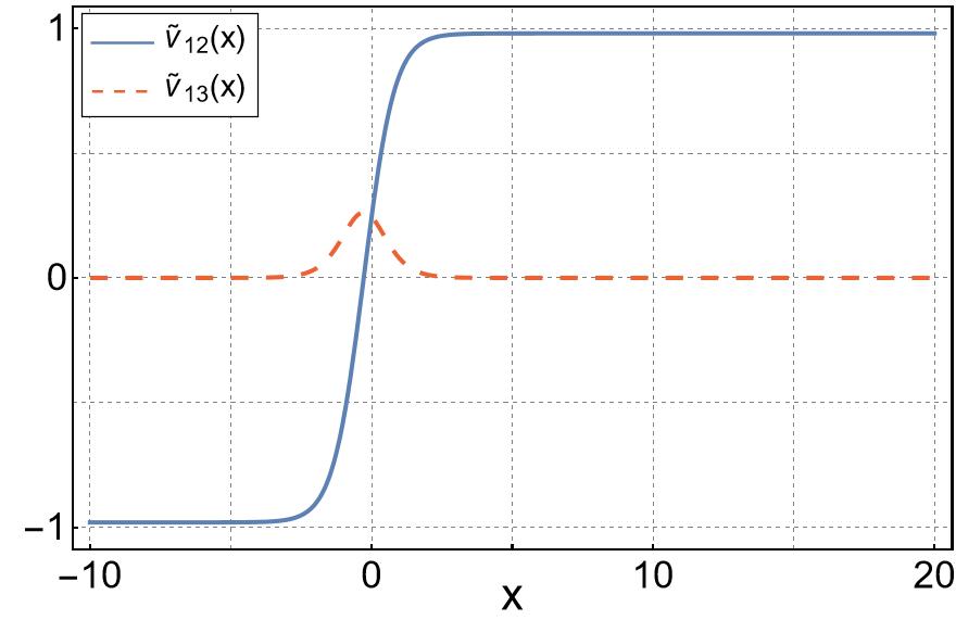
(a)

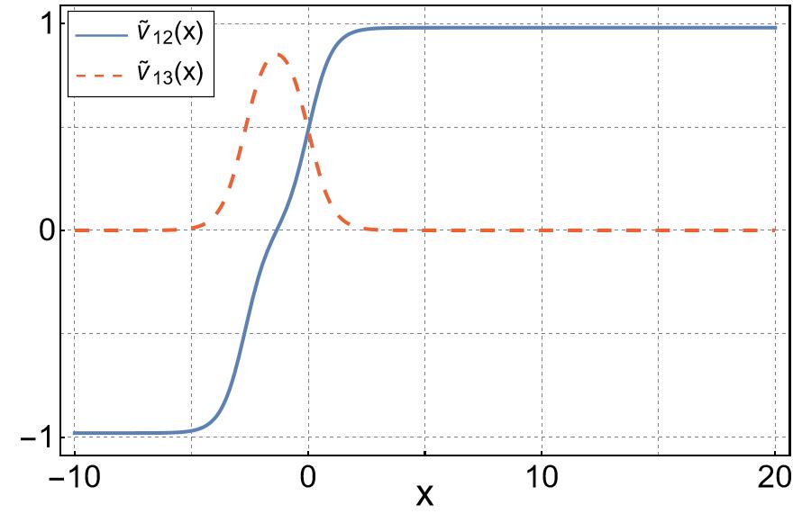
(b)

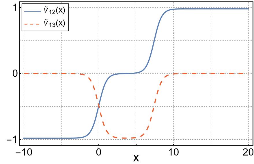
(c)

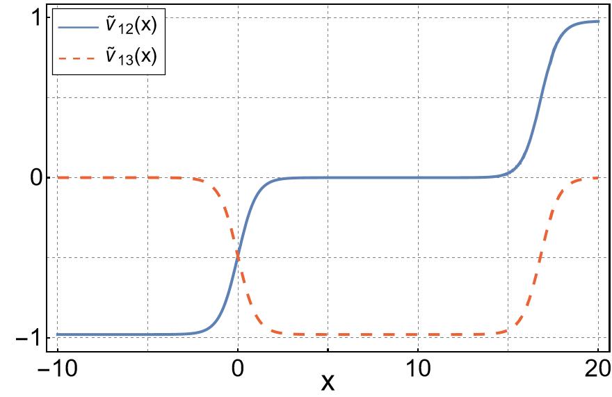
(d)

Figure 2: (Color online) Matrix potential terms $\tilde{v}_{12}(x)$ (blue-solid) and $\tilde{v}_{13}(x)$ (red-dashed)) obtained from (34). Here, the parameters have been fixed to $A=m=0.8$, $\rho=1$, $\lambda=\frac{1}{2}\sqrt{A^{2}+m^{2}}$, combined with $\omega=2\omega_{crit}$ (a), $\omega=(1+10^{-2})\omega_{crit}$ (b), $\omega=-(1+10^{-6})\omega_{crit}$ (c), and d) $\omega=-(1+10^{-14})\omega_{crit}$ (d).

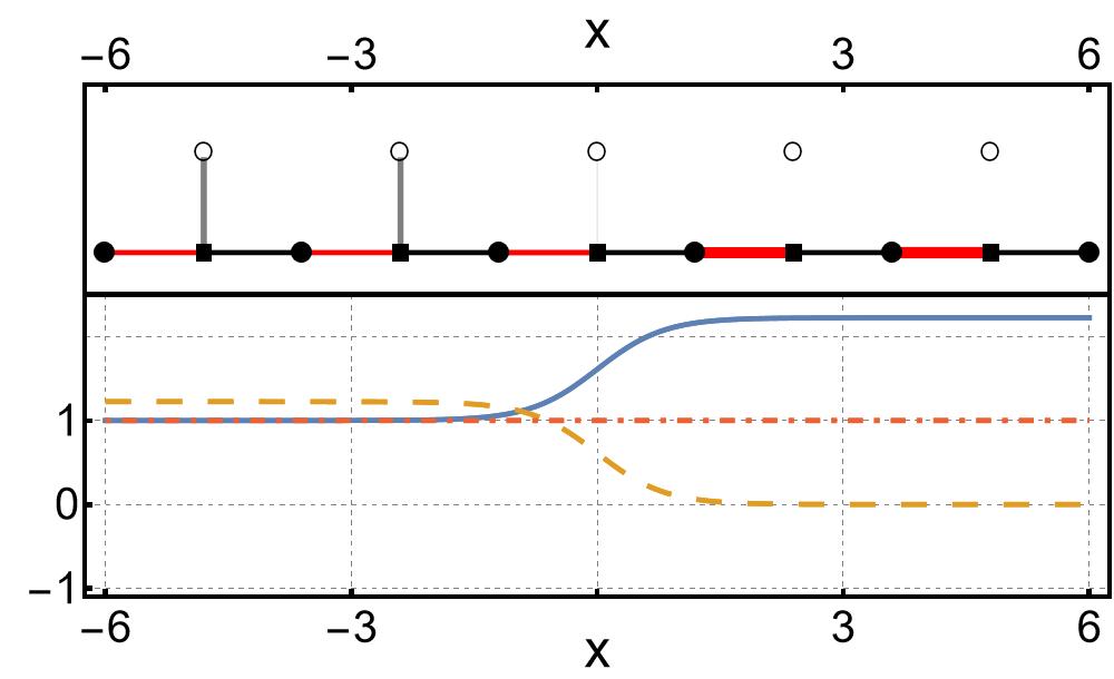
(a)

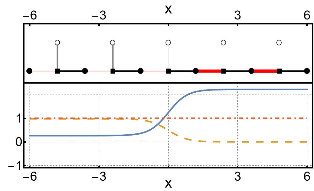
(b)

Figure 3: Inhomogeneous hopping parameters $t_{1}=t_{2}+\tilde{v}_{12}$ (blue-solid), $t_{3}=\tilde{v}_{13}$ (orange-dashed) and $t_{3}$ (red-dot-dashed) for $\omega=\omega_{c}$ computed from (36), (38), and (27). We fixed $t_{2}=1$, $m=1$, $A=1$ and $\rho=1$ (left) and $\rho=0.5$ (right). In the insets, we depict the quasi-one-dimensional chain with the corresponding interactions (the thicker the line, the stronger the coupling), with $t_{1}$ red, $t_{2}$ black, and $t_{3}$ the vertical line.

We can see that $\tilde{v}_{12}$ is changing its sign asymptotically again. The interaction $\tilde{v}_{13}$ acquires non-zero constant value for large negative $x$.

The potential $\tilde{V}$ can be matched with the interaction term of the quasi-one-dimensional chain (27) where the generalized stub lattice gets converted into SSH chain with a parallel chain of non-interacting atoms. The interaction between the two chains is localized in case of (34) while in case of (38), it gets extended over the half-axis. Dimerization pattern on the SSH chain gets changed as the ratio of $t_{1}/t_{2}$ (where $t_{1}=\tilde{v}_{12}+t_{2}$) is inverted along $x$ axis. This way, it resembles the SSH chains with a domain wall. In Fig.3, there is illustrated the case $\omega=\omega_{crit}$, where a semi-infinite generalized stub lattice gets disassembled at the origin into the SSH chain with parallel non-interacting atoms.

Supersymmetric transformation can generate bound states with discrete energies in the new system. The candidates for the new bound states are formed by the columns of the matrix $(U^{\dagger})^{-1}$ that satisfies

$$H_{2}(U^{\dagger})^{-1}=(U^{\dagger})^{-1}\mbox{diag}\{m,\lambda,\lambda\},$$ (41)

see [32]. The eigenstate corresponding to the eigenvalue $m$ is not normalizable. The other two columns are eigenvectors with the eigenvalue $\lambda$. Their explicit form and square integrability is not of our interest. The reason is that $\lambda$ corresponds to the flat-band energy and, therefore, it is infinitely degenerated anyway. Indeed, we can find infinite number of independent normalizable eigenvectors of the form $L(0,0,\xi(x))^{t}$ where $||\xi||<\infty$ ($t$ denotes transposition).

By construction, the spectrum of $\tilde{H_{1}}$ is composed from two energy bands of negative and positive energies. The energy $\lambda$ of the flat band can take any value from the energy gap,

$$\sigma(\tilde{H})=\left(-\infty,-\sqrt{m^{2}+A^{2}}\right]\cup\left[\sqrt{m^{2}+A^{2}},\infty\right)\cup\{\lambda\},\quad\lambda^{2}<m^{2}+A^{2}.$$ (42)

The barrier represented by $\tilde{V}$ in (34) is perfectly transparent. The quasi-particles tunnel through it without being back scattered. It it reminiscent to the Klein tunneling of quasi-particles in graphene through electrostatic barriers. Here, the particles can pass through the barrier without reflection independently on their energy. It can be understood with the use of the intertwining operator $L$ that makes it possible to map the eigenstates of $H_{1}$ into those of $\tilde{H}_{1}$. The Hamiltonian $H_{1}$ corresponds to the free-particle energy operator with a constant potential. Let us suppose that its physical eigenstate $\psi_{k}(x)=e^{ikx}(a,b,c)^{t}$ corresponds to the plane waves with a fixed momentum $k\in\mathbb{R}$. The intertwining operator $L$ converts these states into the scattering states of $\tilde{H}_{1}$. We can write

$$L\psi_{k}(x)=(\partial_{x}-U_{x}U^{-1})e^{ikx}(a,b,c)^{t}=e^{ikx}(ik-U_{x}U^{-1})(a,b,c)^{t},$$ (43)

where $a,b,c$ are complex-valued constant components of the three-component wave function. The matrix $U_{x}U^{-1}$ converges to a constant matrix for large $|x|$. Therefore, $L\psi_{k}(x)$, $|x|\rightarrow\infty$, acquires the form of the plane wave whose momentum is not altered by the potential barrier,

$$\lim_{x\rightarrow\pm\infty}L\psi_{k}(x)=e^{ikx}(\tilde{a}_{\pm},\tilde{b}_{\pm},\tilde{c}_{\pm})^{t},\quad\tilde{a}_{\pm},\tilde{b}_{\pm},\tilde{c}_{\pm}\in\mathbb{C},$$ (44)

i.e. there is no back-scattering.

5 Coexistence of a discrete energy and the flat-band

We start the with following Hamiltonian

$$H_{1}=\begin{pmatrix}M&-i\partial_{x}-im\tanh mx&0\\ -i\partial_{x}+im\tanh mx&-M&0\\ 0&0&\lambda\end{pmatrix},$$ (45)

where $M$, $m$ and $\lambda$ are real constants. The stationary equation $H_{1}\Psi=\epsilon\,\Psi$ is exactly solvable for any $\epsilon$. Indeed, fixing the wave function $\Psi=(\psi,\phi,0)$ and $|\epsilon|\neq M$, the stationary equation decouples into $\phi=-i\frac{\partial_{x}-A}{E+M}\psi$ and $(-\partial_{x}^{2}-\epsilon^{2}+M^{2}+m^{2})\psi=0$. Hence, the upper component is the eigenstate of the Schrödinger Hamiltonian of the free particle. This is due to the fact that the potential term in (45) is related to the reflectionless Pöschl-Teller model, see [55, 56]. The operator $H_{1}$ has a square integrable bound state $\Psi_{-M}$ with energy $-M$,

$$,H_{1}\Psi_{-M}=-M\Psi_{-M},\quad\Psi_{-M}=(0,\mbox{sech}\,mx,0)^{t}.$$ (46)

The elements of the matrix $U$ are fixed in the following manner

$$\psi_{0}=\cosh mx,\quad\psi_{1}=-k\sqrt{m^{2}-k^{2}}\mu(\cosh kx+c_{0}\sinh kx),\quad\psi_{2}=-k\sqrt{m^{2}-k^{2}}\mu\sinh kx,$$ (47)

and

$$\xi_{2}=\cosh\,kx.$$ (48)

The parameter $\mu$ controls reality of these functions, i.e. $\mu=1$ for $k^{2}<m^{2}$ and $\mu=i$ for $k^{2}>m^{2}$. The components $\phi_{1}$ and $\phi_{2}$ can be calculated from $\phi_{a}=-i\frac{\partial_{x}-A}{E+M}\psi_{a}$, $a=1,2$. The energy of flat-band is given as

$$\lambda=\sqrt{M^{2}+m^{2}-k^{2}}.$$ (49)

With this choice of its elements, the matrix $U$ satisfies the following relation.

$$H_{1}U=U\begin{pmatrix}M&0&0\\ 0&\lambda&0\\ 0&0&\lambda\end{pmatrix}.$$ (50)

Using the (17), the components $\tilde{v}_{12}$ and $\tilde{v}_{13}$ of the potential can be calculated as follows,

$$\tilde{v}_{11} =-\lambda$$ (51)

$$\tilde{v}_{12} =-m\tanh mx+(k^{2}-m^{2})\frac{1+\tanh kx(\delta c-k^{2}(M-\lambda)^{2}\mu^{2}\tanh kx)}{d(x)},$$ (52)

$$\tilde{v}_{13} =(M-\lambda)\frac{\mu\sqrt{m^{2}-k^{2}}\,k^{2}\,\mbox{sech}^{2}kx}{d(x)},\quad\delta c=c_{0}-c_{1},$$ (53)

where

$$d(x)= \delta c(k-m\tanh kx\tanh mx)+k\tanh kx-m\tanh mx$$ (54)

$$+k^{2}\mu^{2}(M-\lambda)^{2}\tanh kx\,(k-m\tanh kx\tanh mx).$$ (55)

We shall fix the parameters such that $d(x)$ is non-vanishing. The function is linear in $\delta c$. The terms that do not depend on $\delta c$ are bounded. Let us fix

$$k>m>0,\quad\mu=i.$$

Then the coefficient of $\delta c$ is strictly positive and we can always fix $\delta c$ such that the first term of $d(x)$ is greater than the sum of the remaining terms. This way, we can keep $d(x)>0$.

We are interested in the critical value of $\delta c$. We have

$$d(x) >0\Leftrightarrow\delta c>\frac{m\tanh mx-k\tanh kx}{(k-m\tanh kx\tanh mx)}+k^{2}\,\mu^{2}\,(M^{2}-\lambda^{2})\,\tanh kx\equiv:w(x).$$ (56)

We find that $w(x)$ is an odd and strictly decreasing function,

$$\partial_{x}w(x)=-k^{3}\mbox{sech}^{2}kx\left(\frac{k^{2}-m^{2}}{k^{2}(k-m\tanh kx\tanh mx)^{2}}+(M-\lambda)^{2}\right).$$ (57)

We define the critical value $\delta c_{crit}$ as follows

$$\delta c_{crit}\equiv\lim_{x\rightarrow-\infty}w(x)=1+k^{2}\left(M-\lambda\right)^{2}.$$ (58)

Then both $\tilde{v}_{12}$ and $\tilde{v}_{13}$ are regular for $|\delta c|\geq|\delta c_{crit}|$. The potential term $\tilde{v}_{12}$ changes its sign asymptotically. In the limit of large $|x|$, it has the following behavior,

$$\lim_{x\rightarrow\pm\infty}\tilde{v}_{12}=\mp k.$$ (59)

The explicit form of $\tilde{v}_{12}$ and $\tilde{v}_{13}$ for $|\delta c|>|\delta c_{crit}|$ is in (51). When $\delta c=-\delta c_{crit}$, we have

$$\tilde{v}_{12} =-m\tanh mx+\frac{(k^{2}-m^{2})(1+\tanh kx(1+k^{2}(M-\lambda^{2})(1+\tanh kx)))}{d_{c}(x)},$$ (60)

$$\tilde{v}_{13} =\frac{\sqrt{m^{2}-k^{2}}\,k^{2}\,\mu\,(M-\lambda)\,\mbox{sech}^{2}kx}{d_{c}(x)},$$ (61)

where

$$d_{c}(x)=k\tanh kx-m\tanh mx+(1+k^{2}(M^{2}-\lambda^{2})(1-\mu^{2}\tanh kx))(k-m\tanh kx\tanh mx).$$ (62)

The components $\tilde{v}_{12}$ and $\tilde{v}_{13}$ are depicted explicitly in Fig.5. There is clear similarity with the potential (34). Contrary to that model, the barriers possess an apparent left-right asymmetry.

It is noticeable that the current model supports a bound state with energy $E=-M$. Indeed, by construction, the system has a non-degenerate energy level $E=-M$ with the corresponding bound state

$$\tilde{\Psi}_{-M}=L\,(0,\mbox{sech}mx,0)^{t},\quad\tilde{H}_{1}\tilde{\Psi}_{-M}=-M\tilde{\Psi}_{-M}$$ (63)

The spectrum of this model has the form

$$\sigma(\tilde{H})=\left(-\infty,-\sqrt{M^{2}+m^{2}}\right]\cup\left[\sqrt{M^{2}+m^{2}},\infty\right)\cup\{\sqrt{M^{2}+m^{2}-k^{2}},-M\},$$ (64)

where $|M|>|k|>|m|$, which is further illustrated in Fig. 4.

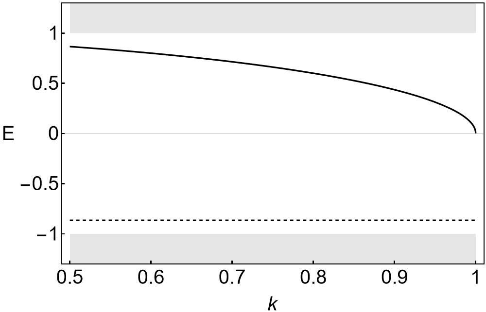
Figure 4: Spectrum of $\tilde{H}_{1}$. For each fixed value $k$, the two shaded bands represent the continuum. The thick black line corresponds to flat-band energy and the thin black line is the energy of the bound state $L\Psi_{-M}$.

The behavior of both $\tilde{v}_{12}$ and $\tilde{v}_{13}$ is sensitive to the proximity of $|\delta c|$ to $|\delta c_{crit}|$. The width of the plateau in the two-step function of the width of the well increases as $|\delta c|$ tends to $|\delta c_{crit}|$. This time, the plateau corresponds to a non-vanishing energy. There is also a bound state $\tilde{\Psi}_{-M}$. In Fig. 5, we present the plots of $\tilde{v}_{12}$ and $\tilde{v}_{13}$ for $\delta c$ that is very close to $\delta c_{crit}$ but with varying $m$ and $M$ such that $M^{2}+m^{2}$ is kept constant. For small values of $m$, $\tilde{v}_{12}$ forms a two-step function that resembles the potential from the previous model, see Fig. 5a), Fig. 5b). As $m$ increases, there is formed a potential well in $\tilde{v}_{12}$, see Fig. 5c) and 5d).

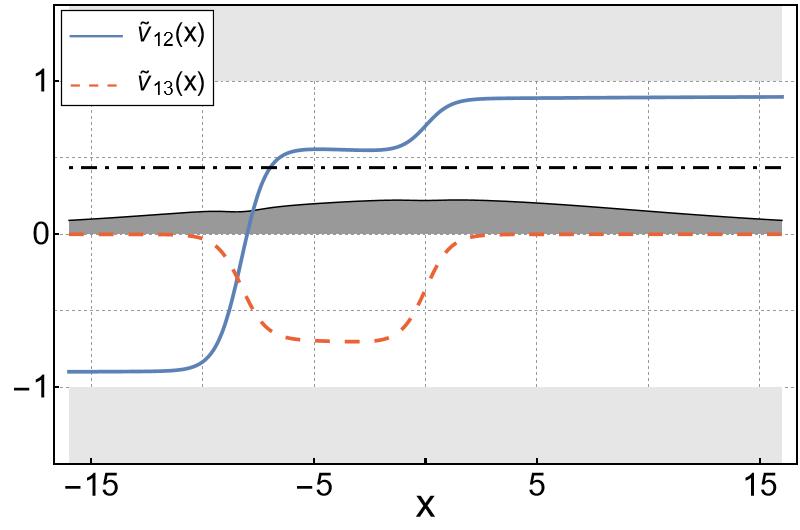
(a)

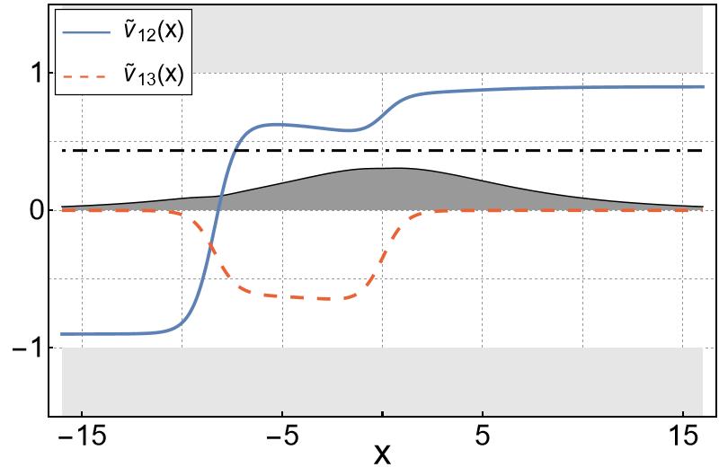
(b)

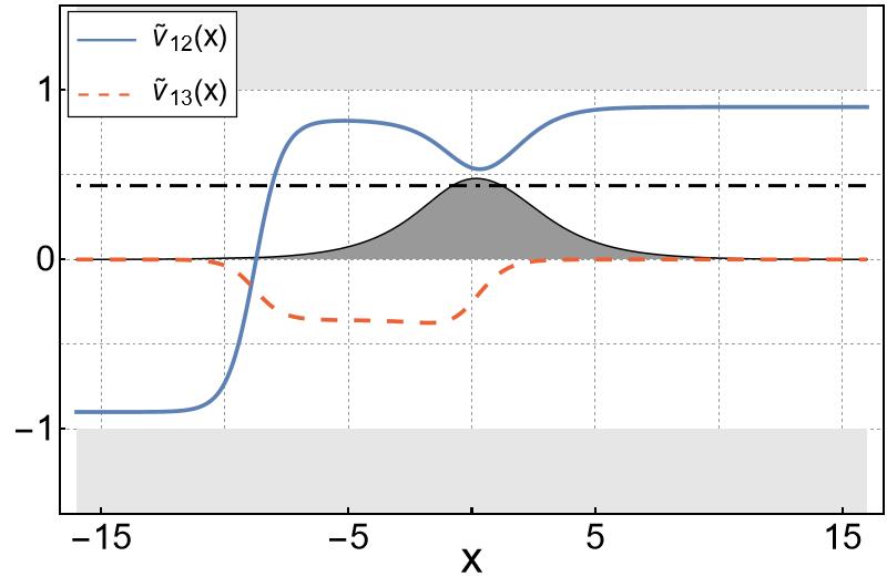
(c)

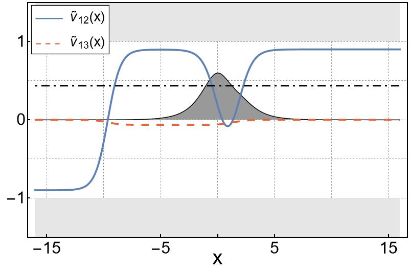
(d)

Figure 5: (color online) Matrix potential elements $\tilde{v}_{12}(x)$ (blue-solid), $\tilde{v}_{13}(x)$ (red-dashed), and the flat-band energy level $\lambda$ (dot-dashed). The rest of parameters have been fixed as $k=0.9$, $M=\sqrt{1-m^{2}}$, $\delta c=1+k^{2}(M-\lambda)+10^{-6}$, together with $m=0.1$ (a), $m=0.2$ (b), $m=0.5$ (c), $m=0.8$ (d). The dark-shaded curve depicts the probability density of the bound state $\tilde{\Psi}_{-M}$.

This is qualitatively different behavior in comparison with the previous model. It is clearly visible when $\delta c=\delta c_{crit}$. The plot of $\tilde{v}_{12}$ and $\tilde{v}_{13}$ in this regime is in Fig. 6. In this figure, there is also the generalized stub lattice with hopping amplitudes $t_{1}$, $t_{2}$ and $t_{3}$ in correspondence with (27).

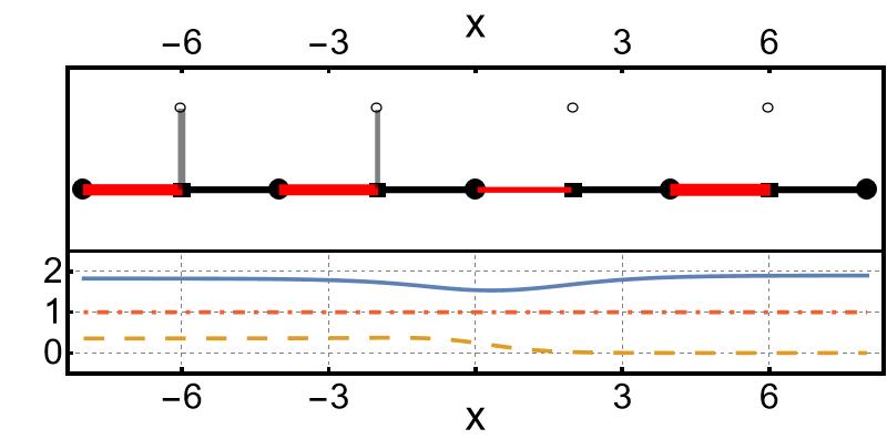
Figure 6: (color online) $t_{1}=t_{2}+\tilde{v}_{12}$ (blue-solid), $t_{3}=\tilde{v}_{13}$ (orange-dashed) and $t_{3}$ (red-dot-dashed) for $\omega=\omega_{c}$, see (36), (38) and (27). We fixed $t_{2}=1$, $m=1$, $A=1$ and $\rho=1$ (left) and $\rho=0.5$ (right). The inset depicts the quasi-one-dimensional chain with the corresponding interactions (the thicker the line, the stronger the coupling).

Discussion of the scattering properties of the model with the potential (51) can be conducted in close analogy with the previous model, i.e. the current setting is also free of back-scattering. Likewise, in the previous model, this property is inherited by $\tilde{H}_{1}$ that is also reflectionless. The matrix $U_{x}U^{-1}$ in the operator $L=\partial_{x}-U_{x}U^{-1}$ tends asymptotically to a constant matrix, and, therefore, the operator $L$ cannot change the momentum of the plane wave that corresponds to the scattering state of $H_{1}$.

6 Discussion

We presented the method for the spectral design of quasi-one-dimensional crystals with flat-band that can be described effectively by the Dirac equation. Our approach is based on the susy transformation of the trivially extended pseudo-spin-one operator $H_{1}$. The later operator is block diagonal with $H_{1/2}$ and a constant on the diagonal. The operator $H_{1/2}$ governs the dynamics of a dimerized chain of atoms. The constant term represents an additional, parallel chain of atoms that are not interacting with their neighbors and host the flat band states. Susy transformation of $H_{1}$ provides us with the operator $\tilde{H}_{1}$ that already possesses non-trivial interaction between the two atomic chains, see (17) or (23). The susy transformation of $H_{1}$ is partially defined in terms of flat-band solutions. The latter functions are selected such that $\tilde{H}_{1}$ is hermitian, see (15).

The method was illustrated by two explicit models where SSH chain interacts locally with a parallel chain of otherwise non-interacting atoms. In the two models, the form of the interaction was tunable via free parameters, see Fig. 2 and Fig. 5. We demonstrated that in the limit where the parameters approach the critical values, the interaction approximates piecewise constant potential, see Fig. 3 and Fig. 6.

The trivial extension of $H_{1/2}$ to $H_{1}$ by diagonal constant $\lambda$ fixes the energy of the flat-band, see (13). The remaining spectral characteristics of $H_{1}$ are inherited from those of $H_{1/2}.$ The spectrum of $H_{1/2}$ itself can also be adjusted by an appropriate susy transformation. The model discussed in Section 5 exemplifies such a situation. Indeed, the block-diagonal operator in (45) can be obtained from the free-particle Hamiltonian via susy transformation that generates the discrete energy $E=-M$ in the spectrum of (45), see [55].

The models described by $\tilde{H}_{1}$ also inherit scattering characteristics of $H_{1}$. Both in Section 4 and in Section 5, $H_{1}$ was fixed as the reflectionless operator. The susy partners $\tilde{H}_{1}$ shared this property as they do not support any backscattering on the potential barriers. This behavior resembles Klein tunneling that occurs in electrostatic field, see the recent analysis in [53].

It is worth noticing that our current work was inspired by [45] where spin-one free particle Dirac operator was transformed by supersymmetric transformation into the new ones with non-trivial potentials. In one specific case, the susy transformation resulted in decoupling of the Hamiltonian, i.e. it acquired block-diagonal form with $2\times 2$, spin-$1/2$ operator and a constant on the diagonal, see [45] for more details. The inverse approach was followed in the current article and exploited in the context of quasi-one-dimensional atomic chains. It is also worth mentioning that the presented construction based on susy transformation of the block-diagonal operators shares the same philosophy with [57] where the interaction between uncoupled systems was induced by unitary transformations.

The proposed approach for spectral design of quasi-one-dimensional systems with flat-bands is very flexible. It is straightforward to adjust it for the construction of quasi-one-dimensional systems with a higher number of flat-bands and/or additional SSH-like chains. The number and energies of the flat-bands can be easily controlled by addition of non-interacting parallel atomic chains to the initial Hamiltonian $H_{1/2}$, i.e. via its trivial extension by corresponding number of diagonal constant terms. The susy transformation would generate the coupling between the original SSH-type chain(s) and the other, initially non-interacting, chains. It would be also possible to consider effects of magnetic field that alters the phase of the hopping parameters. It is worth noticing in this context that generation of the syntetic magnetic field for optical lattices was proposed in [17], [23]. Nevertheless, such analysis of such extensions goes beyond the scope of the present work and should be reported elsewhere.

Appendix A On the structure of the matrix $U$

Let us define the following set of $3\times 3$ matrices

$$\mathbb{M}=\left\{M=\begin{pmatrix}\mathbb{B}&\mathbf{b}\\ \mathbf{0}&\xi\end{pmatrix},\quad\mathbb{B}\in\mathbb{C}^{2\times 2},\quad\mathbf{b}\in\mathbb{C}^{1\times 2},\quad\xi\in\mathbb{C},\quad\mathbf{0}=(0,0)\right\}$$ (A-1)

The set $M$ is closed with respect to matrix multiplication and inverse operation, i.e. it forms a group,

$$M_{1},\ M_{2}\in\mathbb{M}\Rightarrow M_{1}.M_{2}\in\mathbb{M},\ M_{a}^{-1}\in\mathbb{M},\ a=1,2.$$ (A-2)

It is worth noticing that $S_{1}\equiv\begin{pmatrix}0&1&0\\ 1&0&0\\ 0&0&0\end{pmatrix}$ belongs to $\mathbb{M}$. If we select the matrix $U$ such that $U\in\mathbb{M}$, then $U_{x}\in\mathbb{M}$ and we get

$$\delta V=i[S_{1},U_{x}U^{-1}]=\begin{pmatrix}\mathbb{B}&\mathbf{b}\\ \mathbf{0}&0\end{pmatrix}\in\mathbb{M}.$$ (A-3)

It is manifestly non-hermitian. The vector $\mathbf{b}$ can be nullified by a specific choice of the seed solutions. Nevertheless, the new potential $\delta V$ is again block-diagonal.

Therefore, we have to work with two flat-band states at least, fixing the matrix $U$ in this form

$$U=\begin{pmatrix}\mathbf{b}&\mathbb{B}\\ 0&\boldsymbol{\xi}\end{pmatrix},\quad\boldsymbol{\xi}=(\xi_{1},\xi_{2}).$$ (A-4)

In other words, two of the three factorization energies should correspond to the energy (energies) of the flat-band (flat-bands) in order to avoid construction of the new Hamiltonian with undesired block-diagonal structure.

References

- [1] D. Leykam, A. Andreanov, and S. Flach, ”Artificial flat band systems: From lattice models to experiments,” Adv. Phys. X 3, 1473052 (2018).
- [2] Robert Drost et al ”Topological states in engineered atomic lattices,” Nature Phys. 13, 668 (2017).
- [3] M. R. Slot, S. N. Kempkes, E. J. Knol, W. M. J. van Weerdenburg, J. J. van den Broeke, D. Wegner, D. Vanmaekelbergh, A. A. Khajetoorians, C. Morais Smith, and I. Swart, ”p-Band Engineering in Artificial Electronic Lattices,” Phys. Rev. X 9, 011009 (2019).
- [4] L. Yan and P. Liljeroth, ”Engineered electronic states in atomically precise artificial lattices and graphene nanoribbons,” Adv. Phys. X 4, 1651672 (2019).
- [5] Saoirsé E. Freeney et al, ”Electronic Quantum Materials Simulated with Artificial Model Lattices,” ACS Nanosci. Au 2, 198 (2022).
- [6] R. A. Vicencio, C. Cantillano, L. Morales-Inostroza, B. Real, C. Mejía-Cortés, S. Weimann, A. Szameit, and M. I. Molina, ”Observation of Localized States in Lieb Photonic Lattices,” Phys. Rev. Lett. 114, 245503 (2015).
- [7] Bastian Real et al, ”Flat-band light dynamics in Stub photonic lattices,” Scientific Reports 7, 15085 (2017).
- [8] Tian-Xue Ma et al, ”Acoustic flatbands in phononic crystal defect lattices,” J. Appl. Phys. 129, 145104 (2021).
- [9] Pragalv Karki and Jayson Paulose, ”Non-singular and singular flat bands in tunable phononic metamaterials,” Phys. Rev. Research 5, 023036 (2023).
- [10] Md Nurul Huda et al, ”Designer flat bands in quasi-one-dimensional atomic lattices,” Phys. Rev. Res. 2, 043426 (2020).
- [11] Evgenij Travkin, Falko Diebel, Cornelia Denz, ”Compact flat band states in optically induced flatland photonic lattices,” Appl. Phys. Lett. 111, 011104 (2017).
- [12] Eric J. Meier, Fangzhao Alex An, Bryce Gadway, ”Observation of the topological soliton state in the Su–Schrieffer–Heeger model,” Nature Communications 7, 13986 (2016).
- [13] M. N. Huda, S. Kezilebieke, R. Drost, T. Ojanen, and P. Liljeroth, ”Tuneable topological domain wall states in engineered atomic chains,” npj Quantum Mater. 5, 17 (2020).
- [14] Juan Zurita, Charles E. Creffield, Gloria Platero, ”Topology and Interactions in the Photonic Creutz and Creutz-Hubbard Ladders,” Adv. Quantum Tehchnol. 3, 1900105 (2020).
- [15] Dario Bercioux, Omjyoti Dutta, and Enrique Rico, ”Solitons in one-dimensional lattices with a flat band,” Ann. Phys. (Berlin), 1600262 (2017).
- [16] Adamantios Anastasiadis, Georgios Styliaris, Rajesh Chaunsali, Georgios Theocharis, and Fotios K. Diakonos, ”Bulk-edge correspondence in the trimer Su-Schrieffer-Heeger model,” Phys. Rev. B 106, 085109 (2022).
- [17] Stefano Longhi, ”Aharonov–Bohm photonic cages in waveguide and coupled resonator lattices by synthetic magnetic fields,” Optics Letters 39, 5892-5895 (2014).
- [18] Sebabrata Mukherjee, Marco Di Liberto, Patrik Öhberg, Robert R. Thomson, and Nathan Goldman, ”Experimental Observation of Aharonov-Bohm Cages in Photonic Lattices,” Phys. Rev. Lett. 121, 075502 (2018).
- [19] Mark Kremer, Ioannis Petrides, Eric Meyer, Matthias Heinrich, Oded Zilberberg, Alexander Szameit, ”A square-root topological insulator with non-quantized indices realized with photonic Aharonov-Bohm cages,” Nature Communications 11, 907 (2020).
- [20] Amrita Mukherjee, Atanu Nandy, Shreekantha Sil and Arunava Chakrabarti, ”Engineering topological phase transition and Aharonov–Bohm caging in a flux-staggered lattice,” J. Phys.: Condens. Matter 33 035502 (2021).
- [21] S. Shahbazi, M. V. Hosseini, ”Revival of superconductivity in a one-dimensional dimerized diamond lattice,” Sci. Rep. 13, 15725 (2023).
- [22] M. Thumin and G. Bouzerar, ”Flat band superconductivity in a system with a tunable quantum metric: the stub lattice,” Phys. Rev. B 107, 214508 (2023).
- [23] S. Mukherjee, R. Thomson, ”Observation of localized flat-band modes in a quasi-one-dimensional photonic rhombic lattice,” Opt. Lett. 40, 5443 (2015).
- [24] S. Mukherjee, R. Thomson, ”Observation of robust flat-band localization in driven photonic rhombic lattices,” Opt. Lett. 42, 2243-2246 (2017).
- [25] F. Baboux et al, ”Bosonic Condensation and Disorder-Induced Localization in a Flat Band,” Phys. Rev. Lett. 116, 066402 (2016).
- [26] L. Morales-Inostroza and R. A. Vicencio, ”Simple method to construct flat-band lattices,” Phys. Rev. A 94, 043831 (2016).
- [27] Tomonari Mizoguchi and Masafumi Udagawa, ”Flat-band engineering in tight-binding models: Beyond the nearest-neighbor hopping,” Phys. Rev. B 99, 235118 (2019).
- [28] Wulayimu Maimaiti, Alexei Andreanov, Hee Chul Park, Oleg Gendelman, and Sergej Flach, ”Compact localized states and flat-band generators in one dimension,” Phys. Rev. B 95, 115135 (2017).
- [29] Chi-Cheng Lee, Antoine Fleurence, Yukiko Yamada-Takamura, and Taisuke Ozaki, ”Hidden mechanism for embedding the flat bands of Lieb, kagome, and checkerboard lattices in other structures,” Phys. Rev. B 100, 045150 (2019).
- [30] Toshitaka Ogata, Mitsuaki Kawamura, and Taisuke Ozaki, ”Methods for constructing parameter-dependent flat-band lattices,” Phys. Rev. B 103, 205119 (2021).
- [31] F. Cooper, A. Khare and U. Sukhatme, Supersymmetry in quantum mechanics, (World Scientific, Singapore, 2001).
- [32] L. M. Nieto, A. A. Pecheritsin, B. F. Samsonov, “Intertwining technique for the one-dimensional stationary Dirac equation,” Ann. Phys. 305, 151 (2003).
- [33] E. Pozdeeva and A. Schulze-Halberg, “Darboux transformations for a generalized Dirac equation in two dimensions,” Journal of Mathematical Physics 51, 113501 (2010).
- [34] Kuru, S; Negro, J; Nieto, L M, “Exact analytic solutions for a Dirac electron moving in graphene under magnetic fields,” J. Phys. Condens. Matt. 21, 455305 (2009).
- [35] B. Midya, D. J. Fernández, “Dirac electron in graphene under supersymmetry generated magnetic fields,” J. Phys A: Math. Theor. 47, 285302 (2014).
- [36] Anh-Luan Phan, Dai-Nam Le, Van-Hoang Le, Pinaki Roy, “Electronic spectrum of spherical fullerene molecules in the presence of generalized magnetic fields,” Eur. Phys. J. Plus 135, 6 (2020).
- [37] M. Castillo-Celeita, D. J. Fernández, “Dirac electron in graphene with magnetic fields arising from first-order intertwining operators,” J. Phys. A: Math. Theor. 53, 035302 (2020).
- [38] D. J. Fernández J. García, D. O-Campa, “Bilayer graphene in magnetic fields generated by supersymmetry,” J. Phys. A 54, 245302 (2021).
- [39] Axel Schulze-Halberg and Pinaki Roy, “Dirac systems with magnetic field and position-dependent mass: Darboux transformations and equivalence with generalized Dirac oscillators,” Ann. Phys. 431, 168534 (2021).
- [40] Miguel Castillo-Celeita, Alonso Contreras-Astorga, David J. Fernández C., “Complex supersymmetry in graphene,” Eur. Phys.J.Plus 137, 904 (2022).
- [41] Vít Jakubský, Mikhail S. Plyushchay, “Supersymmetric twisting of carbon nanotubes,” Phys. Rev. D 85, 045035 (2012).
- [42] Francisco Correa, Vít Jakubský, “Confluent Crum-Darboux transformations in Dirac Hamiltonians with -symmetric Bragg gratings,” Phys. Rev. A 95, 033807 (2017).
- [43] F. Correa, V. Jakubský, “Twisted kinks, Dirac transparent systems and Darboux transformations,” Phys. Rev. D 90, 125003 (2014).
- [44] A. Contreras-Astorga, F. Correa, and V. Jakubský, “Super-Klein tunneling of Dirac fermions through electrostatic gratings in graphene,” Phys. Rev. B 102, 115429 (2020).
- [45] Vít Jakubský, Kevin Zelaya, ”Reflectionless pseudospin-1 Dirac systems via Darboux transformation and flat band solutions,” Phys. Scr. 99, 035220 (2024).
- [46] W. P. Su, J. R. Schrieffer, and A. J. Heeger, ”Solitons in Polyacetylene,” Phys. Rev. Lett. 42, 1698 (1979).
- [47] A. J. Heeger, S. Kivelson, J. R. Schrieffer, and W. -P. Su, ”Solitons in conducting polymers”, Rev. Mod. Phys. 60, 781 (1988)
- [48] J. K. Asbóth, L. Oroszlány, and A. Pályi, A Short Course on Topological Insulators, Band Structure and Edge States in One and Two Dimensions, 919 (Springer, Cham, 2016).
- [49] Seung-Gyo Jeong and Tae-Hwan Kim, ”Topological and trivial domain wall states in engineered atomic chains,” npj Quantum Materials 7, 22 (2022).
- [50] Seung-Gyo Jeong, Sang-Hoon Han, Tae-Hwan Kim, Sangmo Cheon, ”Revealing inverted chirality of hidden domain wall states in multiband systems without topological transition,” Communications Physics 6, 262 (2023).
- [51] Gerard Queraltó, Mark Kremer, Lukas J. Maczewsky, Matthias Heinrich, Jordi Mompart, Verónica Ahufinger, Alexander Szameit, ”Topological state engineering via supersymmetric transformations,” Commun. Phys. 3, 49 (2020).
- [52] David Viedma, Gerard Queraltó, Jordi Mompart, Verónica Ahufinger, ”High-efficiency topological pumping with discrete supersymmetry transformations,” Opt. Express 30, 23531 (2022).
- [53] Yonatan Betancur-Ocampo, and Guillermo Monsivais, ”Identifying Klein tunneling signatures in bearded SSH lattices from bent flat bands,” arXiv:2312.10621
- [54] Vít Jakubský and Kevin Zelaya, “Landau levels and snake states of pseudo-spin-1 Dirac-like electrons in gapped Lieb lattices,” J. Phys.: Condens. Matter 51, 025302 (2023).
- [55] F. Correa and V. Jakubský, “Twisted kinks, Dirac transparent systems and Darboux transformations,” Phys. Rev. D 90, no.12, 125003 (2014).
- [56] V. Jakubský, “Spectrally isomorphic Dirac systems: Graphene in an electromagnetic field,” Phys. Rev. D 91, 045039 (2015).
- [57] M. Castillo-Celeita, V. Jakubský, ”Reduction scheme for coupled Dirac systems,” J. Phys. A: Math. Theor. 54, 455301 (2021).