Late-time transition of $M_{B}$ inferred via neural networks

Abstract

The strengthening of tensions in the cosmological parameters has led to a reconsideration of fundamental aspects of standard cosmology. The tension in the Hubble constant can also be viewed as a tension between local and early Universe constraints on the absolute magnitude $M_{B}$ of Type Ia supernova. In this work, we reconsider the possibility of a variation of this parameter in a model-independent way. We employ neural networks to agnostically constrain the value of the absolute magnitude as well as assess the impact and statistical significance of a variation in $M_{B}$ with redshift from the Pantheon+ compilation, together with a thorough analysis of the neural network architecture. We find an indication for a transition redshift at the $z\approx 1$ region.

I Introduction

The $\Lambda$CDM concordance model has provided a good description of both astrophysical and cosmological phenomenology for several decades Peebles:2002gy ; Copeland:2006wr . In this regime, cold dark matter (CDM) acts to stabilize galaxies Baudis:2016qwx ; XENON:2018voc while the late time accelerated expansion of the Universe Riess:1998cb ; Perlmutter:1998np is driven by a cosmological constant Mukhanov:991646 . The standard model of cosmology is completed by the inclusion of an inflationary epoch in the very early Universe Guth:1980zm ; Linde:1981mu . On the other hand, the concordance model has several underlying problems that includes the theoretical value of the cosmological constant Weinberg:1988cp , the UV completeness of the theory Addazi:2021xuf , and questions about the direct measurement of CDM particles LUX:2016ggv ; Gaitskell:2004gd . Recently, an observation-driven inconsistency has arisen in which the predictions of the $\Lambda$CDM model for the value of the Hubble constant (based on early Universe measurements) and the value obtained through surveys appear to diverge Abdalla:2022yfr . This Hubble tension is part of a larger cosmological tensions problem in which different cosmological parameters have differing predicted and observed values DiValentino:2020vhf ; DiValentino:2020zio ; DiValentino:2020vvd ; Staicova:2021ajb ; DiValentino:2021izs ; Perivolaropoulos:2021jda ; DiValentino:2022oon ; SajjadAthar:2021prg ; CANTATA:2021ktz ; Colgain:2022tql ; Krishnan:2021jmh ; Anderson:2023aga .

There has been a dramatic increase in the reporting of the divergence of Hubble constant values in recent years. The discrepancy between direct and indirect measurements of $H_{0}$ has reached a critical threshold in statistical significance Aghanim:2018eyx ; ACT:2023kun ; Schoneberg:2022ggi . For the early Universe, the latest reported Hubble constant by the Planck and ACT collaborations are respectively $H_{0}^{\rm P18}=67.4\pm 0.5\,{\rm km\,s}^{-1}{\rm Mpc}^{-1}$ Aghanim:2018eyx and $H_{0}^{\rm ACT-DR4}=67.9\pm 1.5\,{\rm km\,s}^{-1}{\rm Mpc}^{-1}$ ACT:2020gnv . While in the late Universe, direct measurements have produced corresponding values by the SH0ES Team and the Carnegie Supernova Project gives respective reported values of $H_{0}^{\rm S22}=73.5\pm 1.1\,{\rm km\,s}^{-1}{\rm Mpc}^{-1}$ Brout:2022vxf and $H_{0}^{\rm CSP23}=73.22\pm 1.45\,{\rm km\,s}^{-1}{\rm Mpc}^{-1}$ Uddin:2023iob . Other reported values based on strong lensing by TDCOSMO gives a Hubble constant in the range $H_{0}^{\rm TDCOSMO23}=73.3\pm 5.8\,{\rm km\,s}^{-1}{\rm Mpc}^{-1}$ Shajib:2023uig . Each survey shows a high level of internal consistency, the tension arises between survey results, and is particularly poignant for surveys that rely on the $\Lambda$CDM concordance model in making their estimates Bernal:2016gxb .

There has been a diverse range of reactions to the cosmological tensions problem with the prospect of systematics being exceedingly unlikely since the problem has appeared across a wide range of unconnected surveys. To tackle this growing issue, there have been a number of proposals of modifications to the concordance model in which the early Universe Poulin:2023lkg , the neutrino sector DiValentino:2021imh , or the underlying gravitational model Addazi:2021xuf ; CANTATA:2021ktz ; Cai:2019bdh ; LeviSaid:2021yat have been changed. Another approach that is gaining increased interest in the literature is that of using nonparametric approaches to reconstruct the evolution of cosmological parameters using methods that are independent of physical models. Currently, the most studied implementation of these approaches has taken the form of Gaussian processes 10.5555/1162254 which is based on the use of a kernel function that characterizes the covariance relationships between the observed data. The kernels are defined on nonphysical hyperparameters which can then be fit using traditional techniques. There have been a plethora of works in this direction Busti:2014aoa ; Busti:2014dua ; Seikel:2013fda ; Bernardo:2021mfs ; Yahya:2013xma ; 2012JCAP…06..036S ; Shafieloo:2012ht ; Benisty:2020kdt ; Benisty:2022psx ; Bernardo:2021cxi ; Bernardo:2022pyz ; Escamilla-Rivera:2021rbe ; Mukherjee:2021epjc ; Mukherjee:2020vkx ; Shah:2023rqb ; Mukherjee:2023lqr , which includes the reconstruction of various classes of cosmological models Cai:2019bdh ; Bernardo:2021qhu ; Ren:2022aeo ; Briffa:2020qli ; LeviSaid:2021yat . These approaches are interesting but as an approach, Gaussian processes possess several shortfalls in that the reconstructions it produce seem to have an overfitting issue at low values of redshift, as well as an over-reliance on the form of the kernel function.

Another nonparameteric approach that has shown promise in confronting the problem of removing model reliance in data is that of artificial neural network (ANN) 10.2307/j.ctt4cgbdj ; Escamilla-Rivera:2019hqt where the number of nonphysical hyperparameters is dramatically increased and where there is no appearance of the problematic kernel covariance function. In this method, neurons are modeled on their biological analogs, which are then organized into layers that pass signals or inputs through the entirety of the network. This could directly take the form of redshift inputs and Hubble parameter outputs aggarwal2018neural ; Wang:2020sxl ; Gomez-Vargas:2021zyl . One example of an ANN implementation in the cosmological context is Ref. Wang:2019vxv where the Hubble diagram was reconstructed for a number of data sets, this was then further developed in Ref. Dialektopoulos:2021wde to include more complexity in the training data as well as null test analysis of the reconstructions. In Ref. Dialektopoulos:2023dhb this was further solidified with the native inclusion of the underlying covariances in cosmological data forming part of the training process in which the Hubble diagram is produced. ANNs have also been used to devise an approach in which the derivatives of reconstructed parameters, and their associated uncertainties, can be calculated Mukherjee:2022yyq which has led the way to making these methods competitive with Gaussian processes in that they can be used to reconstruct classes of modified cosmological models Dialektopoulos:2023jam .

In this work, we use the robustness of reconstructions based on ANN architectures to probe the potential evolution of the absolute magnitude of type Ia supernovae events (SNIa). It has been suggested in the literature that the Hubble tension may be interpreted as a tension in the absolute magnitude Camarena:2022iae ; Camarena:2021jlr . Indeed, one can certainly transform the Hubble tension into a tension in this value; however, this may imply new physics at the level of the behaviour of astrophysical events. A consequence of this tension in the absolute magnitude would be that one cannot use priors in their analysis of modified cosmological models Efstathiou:2021ocp . Another consequence of this perspective of the tension in the expansion rate of the Universe at present is that one may devise proposals of models through which the absolute magnitude may vary in redshift space. Through this viewpoint, the instrument of nonparametric reconstruction techniques can be used to probe the possible evolution of the absolute magnitude in its own right. Model-independent constraints on the absolute magnitude was attempted by Dinda & Banerjee Dinda:2022jih employing Gaussian processes (GP), where an extensive analysis was carried out with the choice of different kernels and mean functions. As a rigorous extension of Dinda:2022jih , joint constraints on some cosmological nuisance parameters were attempted in Refs. Dinda:2022vmb ; Dinda:2023svr employing different combinations of data sets. Similar efforts in these directions were carried out in Ref. Banerjee:2023evd ; Mukherjee:2021kcu ; Mukherjee:2021epjc . Recent attempts to explore the inherent degeneracy between the parameters, $M_{B}$ and $r_{d}$ (comoving sound horizon at drag epoch) with deep neural networks, was carried out in Ref. Shah:2024slr . Indeed, there have been several physically motivated proposals for the potential evolution of the absolute magnitude parameter coming from phenomena. In Ref. Benisty:2022psx , the constancy of the absolute magnitude was probed comparatively through the reconstruction of the absolute magnitude using three general methods composed of ANNs, two kernel choices of GP reconstruction, and four models taken from the literature Tutusaus:2017ibk ; 2009A&A…506.1095L . Similar efforts to constraining $M_{B}$ or revisiting the constancy of $M_{B}$ in a non-flat universe were carried out by Mukherjee:2020vkx ; Favale:2023lnp for different combinations of datasets. However, results showed no significant evidence to merit an evolution in this parameter. It deserves mention that some of these non-parametric studies employed a combined approach in which baryon acoustic oscillation data (BAO) was used to isolate the luminosity distance and thus infer a value of the absolute magnitude. However, the BAO data is not completely model-independent and may have inserted a preference for this conclusion.

In the current work, we are motivated to reconsider the uncalibrated latest Type Ia supernovae data, namely the Pantheon+ compilation, and use this to reconstruct the apparent magnitudes and their derivatives in a cosmology-independent way using neural networks. Through this route, we can constrain the value of the absolute magnitude $M_{B}$ without making any assumptions on the underlying cosmological model whatsoever. This is achieved by comparing the cosmic chronometer (CC) measurements of the Hubble parameter with the ANN reconstructed Hubble diagram from Pantheon+, thereby computing the absolute magnitude value in an agnostic way. We do this by introducing the technical details of the ANN approach in Sec. II, which directly leads to the reconstruction methodology adopted as detailed in Sec. III. In Sec. IV, we show the cosmology-independent constraints on $M_{B}$ that ANNs can achieve using this approach. Finally, we give a summary of our main conclusions and future work in Sec. V.

II Artificial Neural Networks

In this section, we describe briefly the method by which ANN architectures 2015arXiv151107289C have been adopted. Inspired from biological neural networks, ANNs are built as a collection of neurons which are organized into layers. An input layer, is usually used to enter the data into the network, an output layer is used to extract the parameters we want to learn their behaviour, while there is a series of consecutive layers of neurons in between, usually called hidden layers, that depend on a number of hyperparameters and are being optimized to best mimic the real data processes.

In our case, the input layer will accept redshift values while the output layer gives the supernovae apparent magnitude $m(z)$ for that redshift and its uncertainty. In this way, an input signal, or redshift value, traverses the whole network to train the network, i.e. optimize the hyperparameters of each neuron and then produce these outputs. To illustrate this architecture, we show a two hidden layer ANN for a generic cosmological parameter $\Upsilon(z)$ (which in our case is $m(z)$) and its corresponding uncertainty $\sigma_{\Upsilon}(z)$ (or $\sigma_{m}$ in our case) in Fig. 1, where the neurons are denoted by $\mathfrak{n}_{k}$ and $\mathfrak{m}_{k}$. Here, the ANN is structured so that a linear transformation (composed of linear weights and biases) is applied for each of the different layers.

Figure 1: The adopted ANN architecture is shown, where the input is the redshift of a cosmological parameter $\Upsilon(z)$, and the outputs are the corresponding value and error of $\Upsilon(z)$.

Neurons are triggered by an activation function that, across the larger number of neurons, can be used to model the complex relationships that feature in the data. In our work, we used the Exponential Linear Unit (ELU) 2015arXiv151107289C as the activation function, specified by

$$f(x)=\begin{cases}{x}&\text{if }x>0\\ {\alpha(e^{x}-1)}&\text{if }x\leq 0\end{cases}\,,$$ (1)

where $\alpha$ is a positive hyperparameter that controls the value to which an ELU saturates for negative net inputs, which we set to unity. Besides being continuous and differentiable, this function does not act on positive inputs while negative inputs tend to be closer to unity for more negative input values. The choice of the activation function for the hidden layers usually has to do with the type of the network, i.e. multilayer perceptron, convolutional, recurrent, etc, while the choice for the output layer activation function has to do with the type of the problem (classification or regression); more details can be found in DeepLearning-book .

The linear transformations and activation function produce a huge number of so-called hyperparameters which are nonphysical and can be optimized using training data so that the larger system mimics some physical process as closely as possible. Indeed, the full number of hyperparameters is even larger since there are additional hyperparameters related to the connection of the neurons which drastically increases the freedom of the ANN systems. The process by which training takes place involves these hyperparameters being optimized by comparing the predicted result $\hat{\Upsilon}$ with the real values $\Upsilon$ (training data) so that their difference is minimized. This minimization is called the loss function. This function is minimized by fitting methods, such as gradient descent, which fixes the hyperparameters for specific data sets, or a combination of them. In our work, we adopt Adam’s algorithm 2014arXiv1412.6980K as our optimizer, which is a modification of the gradient descent method that has been shown to accelerate convergence.

The direct absolute difference between the predicted ($\hat{\Upsilon}$) and training ($\Upsilon$) outputs summed for every redshift is called the L1 loss function. This is akin to the log-likelihood function for uncorrelated data in a Markov Chain Monte Carlo (MCMC) analysis and is a very popular choice for ANN architectures. There are other choices such as the mean squared error (MSE) loss function which minimizes the square difference between $\hat{\Upsilon}$ and $\Upsilon$, and the smooth L1 (SL1) loss function which uses a squared term if the absolute error falls below unity and absolute term otherwise; one can see a comparison of different loss functions in Dialektopoulos:2021wde . Thus, it is at the level of the loss function that complexities in the data are inserted into the ANN through optimization in the training of the numerous hyperparameters that make up the system. In our work, we do this by assuming a loss function that is more akin to correlated data when considering log-likelihood functions for MCMC analyses. To that end, we incorporate the covariance matrix $\mathcal{C}$ of a data set by taking a loss function, given as

$${\rm L_{\chi^{2}}}=\sum_{i,j}\left[m_{\rm obs}(z_{i})-m_{\rm pred}(z_{i})\right]^{\text{T}}\mathcal{C}_{ij}^{-1}\left[m_{\rm obs}(z_{j})-m_{\rm pred}(z_{j})\right]\,,$$ (2)

where $\mathcal{C}_{ij}$ is the total noise covariance matrix of the data, which includes the statistical noise and systematics.

ANNs that feature at least one hidden layer can approximate any continuous function for a finite number of neurons, provided the activation function is continuous and differentiable HORNIK1990551 , which means that ANNs are applicable to the setting of cosmological data sets. In this work, we utilize the code for reconstructing functions from data called Reconstruct Functions with ANN (ReFANN) Wang:2019vxv which is based on PyTorch. The code was run on GPUs to speed up the computational time, as well as making use of batch normalization 2015arXiv150203167I prior to every layer which further accelerates the convergence.

III Reconstruction Methdology

In this section we discuss the data sets used in this analysis together with our training and validation strategy for structuring the ANN system. Finally, we lay out the physical framework on which we perform this model-independent constraint analysis on the evolution of $M_{B}$.

III.1 Observational Data sets

As mentioned in the introduction, in this work, we consider two sets of observational data. We consider the latest Pantheon+ compilation for SNIa observations Brout:2021mpj ; Riess:2021jrx ; Scolnic:2021amr from 1701 light curves that represent 1550 distinct SNIa spanning the redshift range $z<2.3$. This data set comprises apparent magnitude measurements $m$ with their associated statistical uncertainties, tabulated at different redshifts. It also includes a covariance matrix detailing the systematic errors or correlations in the measurements.

We also take into account the latest data set of 32 CC $H(z)$ measurements Stern:2009ep ; Moresco:2012jh ; Moresco:2016mzx ; Borghi:2021rft ; Ratsimbazafy:2017vga ; Moresco:2015cya ; Zhang:2012mp , along with the full covariance matrix that includes systematic and calibration errors, as reported in Ref. Moresco:2020fbm . These data do not assume any particular cosmological model, but depend on the differential ages technique between galaxies, covering the redshift range up to $z\sim 2$.

III.2 ANN Training and Validation

Following the prescription outlined in Sec. II, we train our neural network using the Pantheon+ SNIa dataset Brout:2021mpj ; Riess:2021jrx ; Scolnic:2021amr . To optimize the network’s performance, we split the dataset into training (70%) and validation (30%) sets. To incorporate the covariance matrix of the Pantheon+ dataset into the training algorithm, the $\chi^{2}$ loss function, defined in Eq. (2) is minimized. During training, the number of iterations is set to 30,000 at every epoch where a batch size of 32 was considered. The covariance sub-matrices equivalent for every training batch were carefully chosen from the actual data ensuring that these sub-matrices are positive semi-definite.

The left panel of Fig. 2 showcases the respective training and validation losses across different epochs. To identify the best network architecture, we employ an early stopping criterion based on the ongoing comparison with the validation loss. This strategy helps us prevent overfitting and ensures the selection of a model that generalizes well to unseen data. We find that the optimal network configuration features two hidden layers with 128 neurons each.

Our comprehensive approach to training the neural network ensures robust performance in predicting SNIa apparent magnitudes across varying redshifts. To demonstrate the effectiveness of our algorithm, we present the reconstructed mean and 1$\sigma$ uncertainties as functions of redshift $z$ in the right panel of Fig. 2. We employ a Monte Carlo dropout approach Dialektopoulos:2023dhb , which involves running multiple forward passes with dropout during inference, generating a distribution of predictions that accounts for the inherent uncertainty in the model. This method ensures accurate reconstructions and quantifies prediction uncertainties of $m(z)$ at any arbitrary redshifts, making our algorithm a valuable tool for robust cosmological analyses.

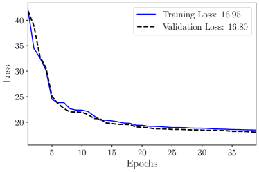
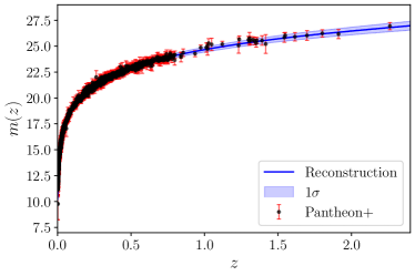
Figure 2: Plots illustrating the evolution of training loss and validation loss across different epochs (left panel). ANN reconstruction of the Pantheon+ SNIa apparent magnitudes $m(z)$ as a function of the redshift $(z)$.

III.3 Theoretical Framework

In a spatially flat Friedmann-Lemaître-Robertson-Walker universe, the luminosity distance is related to the Hubble parameter $H(z)$ at some redshift $z$, as,

$$d_{L}(z)=c(1+z)\int_{0}^{z}\frac{d\tilde{z}}{H(\tilde{z})}.$$ (3)

The observed luminosity of SNIa, from a specific redshift, is related to the apparent peak magnitude $m$ via the following relation, independent of any physical model as,

$$m(z)-M_{B}=5\log_{10}\left[\frac{d_{L}(z)}{\text{1 Mpc}}\right]+25\,.$$ (4)

From Eq. (4), we can rewrite the luminosity distance as,

$$d_{L}(z)=10^{\frac{1}{5}\left[m(z)-M_{B}-25\right]}.$$ (5)

Furthermore, we can compute $d_{L}^{\prime}$, the first order derivative of $d_{L}$ with respect to the redshift $z$ as,

$$d_{L}^{\prime}(z)=\frac{\log(10)}{5}10^{-\frac{M_{B}}{5}}m^{\prime}(z).$$ (6)

Combining Eq. (5) and Eq. (6) with Eq. (3), we can express the Hubble parameter as,

$$H(z)=\frac{c(1+z)^{2}}{(1+z)d_{L}^{\prime}(z)-d_{L}(z)}.$$ (7)

In this way, we can derive the Hubble parameter $H(z)$, from the Pantheon+ apparent magnitudes $m$ and its corresponding derivatives $m^{\prime}$ employing specific values of $M_{B}$. A similar approach is used in the following section in order to get constraints on $M_{B}$ in a cosmological model-independent way.

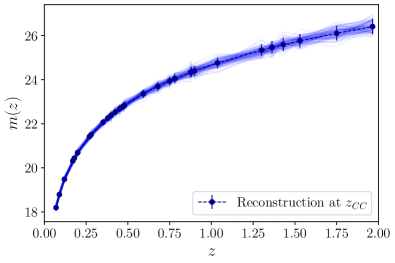
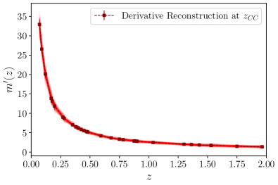
Figure 3: ANN reconstruction of the Pantheon+ apparent magnitudes $m(z)$ at the CC redshifts $(z_{\text{CC}})$.

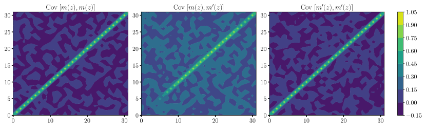
Figure 4: Normalized covariance matrix between ANN reconstruction of the Pantheon+ SN-Ia apparent magnitudes $m(z)$ at the CC redshifts $(z_{\text{CC}})$.

IV Results and Discussions

The ANN architecture is configured in the preceding section with a focus on producing a robust architecture that can reconstruct the possible evolution of $M_{B}$. Here we perform this analysis by using the evolution profiles that the ANN produces. Firstly, our interest is in determining a constant value for the absolute luminosity, and secondly, we explore the possibility of a free evolution through which it turns out that a mild preference for a transition point is determined.

IV.1 Constraints on $M_{B}$

With our trained network model, we proceed to reconstruct $m$ and its 1$\sigma$ uncertainty $\Delta m$ at the CC redshifts. We also obtain the derivatives of $m$ at the respective redshifts, hereafter denoted as $m^{\prime}$, directly employing the automatic differentiation module (namely torch.autograd.grad) to the distribution of predictions obtained during inference. This approach thus helps to simultaneously compute the mean and 1$\sigma$ uncertainty of the reconstructed functions. The plots for the reconstructed $m(z_{\text{CC}})$ and $m^{\prime}(z_{\text{CC}})$ is shown in Fig. 3. Here we also show the distribution of $n$-predicted $m(z)$ and $m^{\prime}(z)$ ANN reconstruction samples. For illustration, we have set $n$=100. The normalized covariance matrices between the reconstructed functions can be visualized from Fig. 4.

For these $n$-reconstructed $m$ and $m^{\prime}$, one can write down the corresponding Hubble parameter as a function of $M_{B}$ utilizing Eq. (7). Finally, to obtain the model-independent constraints on $M_{B}$ we define this $\chi^{2}$ function,

$$\chi^{2}\left\{M_{B}\right\}=\sum_{i,j}\left[H_{\text{CC}}(z_{i})-H_{\text{ANN}}(z_{i})\right]^{\text{T}}\Sigma^{-1}_{ij}\left[H_{\text{CC}}(z_{j})-H_{\text{ANN}}(z_{j})\right]\,.$$ (8)

The corresponding log-likelihood is thus given by,

$$\log\mathcal{L}\left\{M_{B}\right\}=-\frac{\chi^{2}}{2}-\frac{1}{2}\log|\Sigma|-\frac{N}{2}\log(2\pi)\,,$$ (9)

where $N=32$, the size of the CC data. Instead of opting for a $\chi^{2}$ minimization, we undertake a Markov Chain Monte Carlo analysis, where we maximize the log-likelihood by minimizing the negative log-likelihood considering a uniform prior for $M_{B}\in[-21,-18]$.

Initially, we start with $n$=100 ANN-predictions of $m(z_{\text{CC}})$ and $m^{\prime}(z_{\text{CC}})$. Furthermore, we increase $n$ iteratively in steps of 100 up to $n=500$, i.e., $n$=100, 200, 300, 400, 500 respectively. We find that the resulting constraint on $M_{B}$ is slightly dependent on $n$, the total number of ANN reconstructions for $m(z)$ considered, as illustrated in Fig. 5, where a statistically stable value of $M_{B}=-19.353^{+0.073}_{-0.078}$ was reached at around $n=300$ predictions.

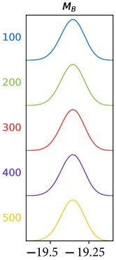
Figure 5: Marginalized posteriors of supernovae apparent magnitude $M_{B}$ as a function of the number of considered ANN reconstructions. The obtained constraints obtained are $M_{B}$ = $-19.352^{+0.073}_{-0.079}$, $-19.352^{+0.073}_{-0.079}$, $-19.353^{+0.073}_{-0.078}$, $-19.353^{+0.073}_{-0.078}$, and $-19.353^{+0.073}_{-0.078}$, corresponding to 100, 200, 300, 400, and 500 ANN reconstructions.

There have been similar efforts to compute $M_{B}$ from different combinations of different cosmological observations Camarena:2019rmj ; Dinda:2022jih ; Banerjee:2023evd ; Favale:2023lnp ; Mukherjee:2021epjc ; Shah:2024slr ; Gomez-Valent:2021hda ; Mukherjee:2021kcu . For a comparative analysis, we mention some of the previous results, for a given set of observational data, in Table 1. Finally, a whisker plot is shown with the available results in Fig. 6 for better illustration. We find that our results are consistent with the constraints on $M_{B}$ obtained from almost all the previous analyses, particularly when similar data sets are taken into consideration Mukherjee:2021epjc ; Dinda:2022jih ; Mukherjee:2021kcu . It deserves to mention that the constraints on $M_{B}$ are tighter when the BAO observations are combined with the CC and SNIa data. This is because the uncertainty associated with the BAO data set is significantly smaller in comparison to the CC data set. However, in this work, we refrain from including the BAO data sets because there are apprehensions regarding their dependence towards some fiducial cosmological model. So, we undertake this analysis utilizing only the SNIa and CC data sets to ensure a complete model-independent prescription.

Reference	Methodology	Datasets	$M_{B}$
Camarena & MarraCamarena:2019rmj	Cosmography	$\alpha_{\text{BAO}}$ + $r_{d}^{\text{CMB}}$ + Pantheon	$-19.401\pm 0.027$
		$\theta_{\text{BAO}}$ + $r_{d}^{\text{CMB}}$ + Pantheon	$-19.262\pm 0.030$
Mukherjee & MukherjeeMukherjee:2021kcu	Gaussian Process	CC + Pantheon	$\mathbf{-19.387\pm 0.060}$
Mukherjee & BanerjeeMukherjee:2021epjc	Gaussian Process	CC + Pantheon	$\mathbf{-19.360\pm 0.059}$
		CC + $r_{\text{BAO}}$ + Pantheon	$-19.398\pm 0.041$
Dinda & BanerjeeDinda:2022jih	Gaussian Process	CC + Pantheon	$\mathbf{-19.384\pm 0.052}$
		BAO + Pantheon	$-19.396\pm 0.016$
		CC + BAO + Pantheon	$-19.395\pm 0.015$
Benisty et al.Benisty:2022psx	Neural Networks	$\alpha_{\text{BAO}}$ + $r_{d}^{\text{CMB}}$ + Pantheon	$-19.38\pm 0.20$
		$\alpha_{\text{BAO}}$ + $r_{d}^{\text{SH0ES}}$ + Pantheon	$-19.22\pm 0.20$
Gómez-ValentGomez-Valent:2021hda	Index of Inconsistency	CC + BAO + Pantheon	$-19.374\pm 0.080$
		CC + BAO + Pantheon ($\Omega_{k}\neq 0$)	$-19.362^{+0.078}_{-0.067}$
Favale et al.Favale:2023lnp	Gaussian Process	CC + Pantheon+	$-19.344^{+0.116}_{-0.090}$
		CC + BAO + Pantheon+	$-19.314^{+0.086}_{-0.108}$
		CC + SH0ES + Pantheon+	$-19.252^{+0.024}_{-0.036}$
		CC + BAO + SH0ES + Pantheon+	$-19.252^{+0.024}_{-0.036}$
Banerjee et al.Banerjee:2023evd	Gaussian Process	CC + $r_{\text{BAO}}$ + Pantheon+ ($\Omega_{k}\neq 0$)	$-19.404^{+0.099}_{-0.104}$
Shah et al.Shah:2024slr	Neural Networks	Pantheon + $\alpha_{\text{BAO}}$ + $r_{d}^{\text{CMB}}$	$-19.394^{+0.018}_{-0.017}$
		Pantheon + $\theta_{\text{BAO}}$ + $r_{d}^{\text{CMB}}$	${-19.257}^{+0.028}_{-0.027}$
This work⋆	Neural Networks	CC & Pantheon+	$\mathbf{-19.353^{+0.073}_{-0.078}}$

Table 1: Comparison between the model-independent constraints on $M_{B}$ obtained in this work vs those present in the literature.

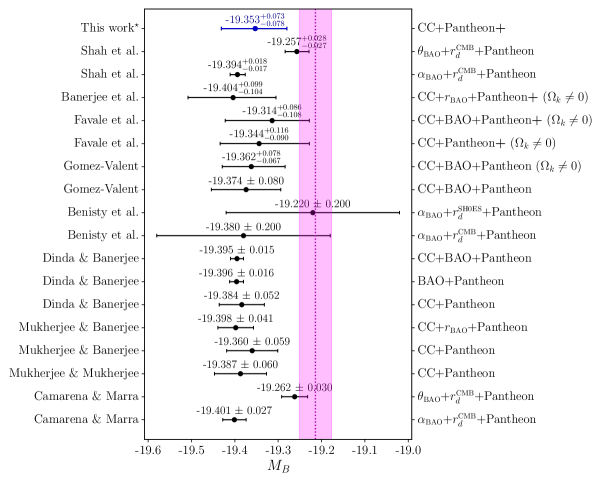
Figure 6: Whisker plot showing a comparison between the model-independent constraints on $M_{B}$ obtained in this work vs those present in the existing literature. The purple region corresponds to the $1-\sigma$ model independent constraint $M_{B}=-19.214\pm 0.037$, as reported in Ref. Riess:2020fzl ; Riess:2021jrx inferred from the Pantheon and SH0ES data sets.

IV.2 Data-driven transition of $M_{B}$

We now investigate the possibility of a redshift evolution in $M_{B}$ by considering two types of binning methods, applied to the adopted $H(z)$ CC data which was already used in Sec. IV.1. The first binning method is the so-called cumulative binning technique Hu:2022kes , in which the next redshift bin has one more high-redshift $H(z)$ data point with respect to the previous redshift bin. To be able to run the MCMC analysis, in our first cumulative redshift bin, we considered the first six low-redshift $H(z)$ data points up to $z_{\mathrm{max}}=0.1993$. The derived values of $M_{B}(z_{\mathrm{max}})$ from the cumulative binning method are shown in Fig. 7, where $M_{B}(z_{\mathrm{max}})$ denotes the value of $M_{B}$ inferred from the $H(z)$ data set with maximal redshift $z_{\mathrm{max}}$.

The other binning strategy that is considered in this work is the approach of conducting the MCMC analysis to determine $M_{B}$ by considering redshift layers Pasten:2023rpc , where each layer has a mean redshift $\bar{z}$. In our analyses, we have considered four layers with $\bar{z}=[0.275,\,0.746,\,1.234,\,1.748]$, and within each redshift layer we have inferred a redshift-dependent constraint on $M_{B}$ as outlined in Table 2.

From the outcomes of the redshift-dependent constraints of $M_{B}$, it should be remarked that there is an indication of a transition in the value of $M_{B}$ at $z\approx 1$, irrespective of the binning techniques adopted.

$\bar{z}$	$M_{B}(\bar{z})$
0.275	$-19.404^{+0.097}_{-0.104}$
0.746	$-19.61^{+0.15}_{-0.16}$
1.234	$-19.14^{+0.14}_{-0.15}$
1.748	$-19.46\pm 0.22$

Table 2: Inferred constraints on $M_{B}(\bar{z})$ using the redshift layers binning technique.

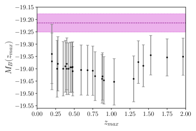
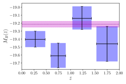
Figure 7: Predictions of the supernovae apparent magnitudes: $M_{B}(z_{\mathrm{max}})$ by adopting cumulative binning, where $M_{B}(z_{\mathrm{max}})$ is the derived value of $M_{B}$ by considering CC $H(z)$ data up to $z_{\mathrm{max}}$ (left panel), and $M_{B}(\bar{z})$ by adopting the redshift layer binning, where $M_{B}(\bar{z})$ is the derived value of $M_{B}$ by considering CC $H(z)$ data within that redshift layer with a mean redshift $\bar{z}$ (right panel). The purple region corresponds to the $1-\sigma$ model independent constraint $M_{B}=-19.214\pm 0.037$, as reported in Ref. Riess:2020fzl ; Riess:2021jrx inferred from the Pantheon and SH0ES data sets.

V Conclusion

In the usual practice, when one estimates cosmic distances as a function of the scale factor and its derivatives, the luminosity of type Ia supernovae is considered a standard candle, which is of utmost importance to understanding the accelerating expansion of the Universe. In this work, we have tried to investigate if this assumption is as educated as it sounds, by constraining the peak absolute magnitude, $M_{B}$, of SNIa, in a cosmological model-independent way. For this exercise, we have utilized two distinct sets of observational data, namely the Pantheon+ SNIa compilation and the cosmic chronometer Hubble parameter measurement, as described in Sec. III.1

In this work we explore the nature of the absolute magnitude parameter through the use of ANNs with a focus on obtaining a model-independent value of this parameter, as well as an indication of whether the parameter expresses a statistically relevant evolution. Using Eq. 7, we show how the Pantheon+ sample can be used to determine the Hubble parameter at different redshift points. This is then used in conjunction with the CC Hubble parameter observations to constrain the value of $M_{B}$ in a model-independent way using the log-likelihood defined in Eq. 9. As shown in Table 1, the final constraint on $M_{B}$ is competitive with other literature values, and moreover, this approach had the advantage that it does not depend on a fiducial cosmological model.

Since the focus is on constraining $M_{B}$ in a model-agnostic way, we do not consider any parametric or theoretical form between $d_{L}$ and $H(z)$ at the outset. Hence, once the observed apparent magnitudes $m$ of the SNIa are given, we proceed to reconstruct $m(z)$ a function of the redshift employing Artificial Neural Networks (Sec. III.2). Utilizing the equations in Sec. III.3, the analogous Hubble parameter, inferred from SN-Ia via Eq. (7), can in principle be written as a function of its peak absolute magnitude $M_{B}$. Finally, having defined the $\chi^{2}$ function for $M_{B}$ (Eq. (8)), we obtain constraints by minimizing the negative log-likelihood in Eq. (9). The result we get is

$$M_{B}=-19.353^{+0.073}_{-0.078}\,.$$ (10)

Furthermore, we proceed to test the evolution of the peak absolute magnitude $M_{B}$ as a function of redshift. For this exercise, two types of binning methods have been adopted while working with the CC data. In the first one, we used the cumulative method, in which a redshift bin has one more data point with respect to the previous bin and the results are shown in Fig. 7. In the second one, we considered four distinct binning of redshifts, where each one has a mean redshift $\bar{z}$, and the results are presented in Table 2. In both cases, one can notice a transition in the value of $M_{B}$ at $z\approx 1$.

More broadly, previous works in the literature open the possibility of a transition redshift over which some parameters may suffer a change in value which includes the $M_{B}$ parameter. Ref. Akarsu:2023mfb ; Paraskevas:2024ytz points to a sign switch from negative to positive in the cosmological constant, while Ref. Perivolaropoulos:2021bds indicates a value transition in $M_{B}$ albeit at a much closer distance. Indeed, even a regular MCMC albeit with a binning procedure will produce a variety of $H_{0}$ values as shown in Refs. Colgain:2023bge ; Colgain:2022tql which may ultimately be interpreted as a variation in the $M_{B}$ parameter.

Indications in the literature have pointed to a variation in the value of $M_{B}$ Efstathiou:2021ocp ; Camarena:2022iae ; Camarena:2021jlr which may represent the underlying physical nature of the tension in terms of astrophysics. The problem of the source and characterization of the $H_{0}$ tension may express other important features relevant for further study. In future work, we hope to apply this new approach to assessing the evolution profile of other important parameters that contribute to constraints on the value of the Hubble constant.

- (1) P. J. E. Peebles and B. Ratra, “The Cosmological Constant and Dark Energy,” Rev. Mod. Phys. 75 (2003) 559–606, arXiv:astro-ph/0207347.
- (2) E. J. Copeland, M. Sami, and S. Tsujikawa, “Dynamics of dark energy,” Int. J. Mod. Phys. D 15 (2006) 1753–1936, arXiv:hep-th/0603057.
- (3) L. Baudis, “Dark matter detection,” J. Phys. G 43 (2016) no. 4, 044001.
- (4) XENON Collaboration, E. Aprile et al., “Dark Matter Search Results from a One Ton-Year Exposure of XENON1T,” Phys. Rev. Lett. 121 (2018) no. 11, 111302, arXiv:1805.12562 [astro-ph.CO].
- (5) Supernova Search Team Collaboration, A. G. Riess et al., “Observational evidence from supernovae for an accelerating universe and a cosmological constant,” Astron. J. 116 (1998) 1009–1038, arXiv:astro-ph/9805201.
- (6) Supernova Cosmology Project Collaboration, S. Perlmutter et al., “Measurements of and from 42 high redshift supernovae,” Astrophys. J. 517 (1999) 565–586, arXiv:astro-ph/9812133.
- (7) V. Mukhanov, Physical Foundations of Cosmology. Cambridge Univ. Press, Cambridge, 2005. https://cds.cern.ch/record/991646.
- (8) A. H. Guth, “The Inflationary Universe: A Possible Solution to the Horizon and Flatness Problems,” Phys. Rev. D 23 (1981) 347–356.
- (9) A. D. Linde, “A New Inflationary Universe Scenario: A Possible Solution of the Horizon, Flatness, Homogeneity, Isotropy and Primordial Monopole Problems,” Phys. Lett. B 108 (1982) 389–393.
- (10) S. Weinberg, “The Cosmological Constant Problem,” Rev. Mod. Phys. 61 (1989) 1–23.
- (11) A. Addazi et al., “Quantum gravity phenomenology at the dawn of the multi-messenger era—A review,” Prog. Part. Nucl. Phys. 125 (2022) 103948, arXiv:2111.05659 [hep-ph].
- (12) LUX Collaboration, D. S. Akerib et al., “Results from a search for dark matter in the complete LUX exposure,” Phys. Rev. Lett. 118 (2017) no. 2, 021303, arXiv:1608.07648 [astro-ph.CO].
- (13) R. J. Gaitskell, “Direct detection of dark matter,” Ann. Rev. Nucl. Part. Sci. 54 (2004) 315–359.
- (14) E. Abdalla et al., “Cosmology intertwined: A review of the particle physics, astrophysics, and cosmology associated with the cosmological tensions and anomalies,” JHEAp 34 (2022) 49–211, arXiv:2203.06142 [astro-ph.CO].
- (15) E. Di Valentino et al., “Snowmass2021 - Letter of interest cosmology intertwined I: Perspectives for the next decade,” Astropart. Phys. 131 (2021) 102606, arXiv:2008.11283 [astro-ph.CO].
- (16) E. Di Valentino et al., “Snowmass2021 - Letter of interest cosmology intertwined II: The hubble constant tension,” Astropart. Phys. 131 (2021) 102605, arXiv:2008.11284 [astro-ph.CO].
- (17) E. Di Valentino et al., “Cosmology intertwined III: and ,” Astropart. Phys. 131 (2021) 102604, arXiv:2008.11285 [astro-ph.CO].
- (18) D. Staicova, “Hints of the tension in uncorrelated Baryon Acoustic Oscillations dataset,” in 16th Marcel Grossmann Meeting on Recent Developments in Theoretical and Experimental General Relativity, Astrophysics and Relativistic Field Theories. 11, 2021. arXiv:2111.07907 [astro-ph.CO].
- (19) E. Di Valentino, O. Mena, S. Pan, L. Visinelli, W. Yang, A. Melchiorri, D. F. Mota, A. G. Riess, and J. Silk, “In the realm of the Hubble tension—a review of solutions,” Class. Quant. Grav. 38 (2021) no. 15, 153001, arXiv:2103.01183 [astro-ph.CO].
- (20) L. Perivolaropoulos and F. Skara, “Challenges for CDM: An update,” New Astron. Rev. 95 (2022) 101659, arXiv:2105.05208 [astro-ph.CO].
- (21) E. Di Valentino, W. Giarè, A. Melchiorri, and J. Silk, “Health checkup test of the standard cosmological model in view of recent cosmic microwave background anisotropies experiments,” Phys. Rev. D 106 (2022) no. 10, 103506, arXiv:2209.12872 [astro-ph.CO].
- (22) M. Sajjad Athar et al., “Status and perspectives of neutrino physics,” Prog. Part. Nucl. Phys. 124 (2022) 103947, arXiv:2111.07586 [hep-ph].
- (23) CANTATA Collaboration, E. N. Saridakis et al., “Modified Gravity and Cosmology: An Update by the CANTATA Network,” arXiv:2105.12582 [gr-qc].
- (24) E. O. Colgáin, M. M. Sheikh-Jabbari, and R. Solomon, “High redshift CDM cosmology: To bin or not to bin?,” Phys. Dark Univ. 40 (2023) 101216, arXiv:2211.02129 [astro-ph.CO].
- (25) C. Krishnan, R. Mohayaee, E. O. Colgáin, M. M. Sheikh-Jabbari, and L. Yin, “Hints of FLRW breakdown from supernovae,” Phys. Rev. D 105 (2022) no. 6, 063514, arXiv:2106.02532 [astro-ph.CO].
- (26) R. I. Anderson, N. W. Koblischke, and L. Eyer, “Reconciling astronomical distance scales with variable red giant stars,” arXiv:2303.04790 [astro-ph.CO].
- (27) Planck Collaboration, N. Aghanim et al., “Planck 2018 results. VI. Cosmological parameters,” Astron. Astrophys. 641 (2020) A6, arXiv:1807.06209 [astro-ph.CO]. [Erratum: Astron.Astrophys. 652, C4 (2021)].
- (28) ACT Collaboration, M. S. Madhavacheril et al., “The Atacama Cosmology Telescope: DR6 Gravitational Lensing Map and Cosmological Parameters,” arXiv:2304.05203 [astro-ph.CO].
- (29) N. Schöneberg, L. Verde, H. Gil-Marín, and S. Brieden, “BAO+BBN revisited — growing the Hubble tension with a 0.7 km/s/Mpc constraint,” JCAP 11 (2022) 039, arXiv:2209.14330 [astro-ph.CO].
- (30) ACT Collaboration, S. Aiola et al., “The Atacama Cosmology Telescope: DR4 Maps and Cosmological Parameters,” JCAP 12 (2020) 047, arXiv:2007.07288 [astro-ph.CO].
- (31) D. Brout et al., “The Pantheon+ Analysis: Cosmological Constraints,” Astrophys. J. 938 (2022) no. 2, 110, arXiv:2202.04077 [astro-ph.CO].
- (32) S. A. Uddin et al., “Carnegie Supernova Project-I and -II: Measurements of using Cepheid, TRGB, and SBF Distance Calibration to Type Ia Supernovae,” arXiv:2308.01875 [astro-ph.CO].
- (33) A. J. Shajib et al., “TDCOSMO. XII. Improved Hubble constant measurement from lensing time delays using spatially resolved stellar kinematics of the lens galaxy,” Astron. Astrophys. 673 (2023) A9, arXiv:2301.02656 [astro-ph.CO].
- (34) J. L. Bernal, L. Verde, and A. G. Riess, “The trouble with ,” JCAP 10 (2016) 019, arXiv:1607.05617 [astro-ph.CO].
- (35) V. Poulin, T. L. Smith, and T. Karwal, “The Ups and Downs of Early Dark Energy solutions to the Hubble tension: a review of models, hints and constraints circa 2023,” arXiv:2302.09032 [astro-ph.CO].
- (36) E. Di Valentino and A. Melchiorri, “Neutrino Mass Bounds in the Era of Tension Cosmology,” Astrophys. J. Lett. 931 (2022) no. 2, L18, arXiv:2112.02993 [astro-ph.CO].
- (37) Y.-F. Cai, M. Khurshudyan, and E. N. Saridakis, “Model-independent reconstruction of gravity from Gaussian Processes,” Astrophys. J. 888 (2020) 62, arXiv:1907.10813 [astro-ph.CO].
- (38) J. Levi Said, J. Mifsud, J. Sultana, and K. Z. Adami, “Reconstructing teleparallel gravity with cosmic structure growth and expansion rate data,” JCAP 06 (2021) 015, arXiv:2103.05021 [astro-ph.CO].
- (39) C. E. Rasmussen and C. K. I. Williams, Gaussian Processes for Machine Learning (Adaptive Computation and Machine Learning). The MIT Press, 2005.
- (40) V. C. Busti, C. Clarkson, and M. Seikel, “The Value of from Gaussian Processes,” IAU Symp. 306 (2014) 25–27, arXiv:1407.5227 [astro-ph.CO].
- (41) V. C. Busti, C. Clarkson, and M. Seikel, “Evidence for a Lower Value for from Cosmic Chronometers Data?,” Mon. Not. Roy. Astron. Soc. 441 (2014) 11, arXiv:1402.5429 [astro-ph.CO].
- (42) M. Seikel and C. Clarkson, “Optimising Gaussian processes for reconstructing dark energy dynamics from supernovae,” arXiv:1311.6678 [astro-ph.CO].
- (43) R. C. Bernardo and J. Levi Said, “Towards a model-independent reconstruction approach for late-time Hubble data,” JCAP 08 (2021) 027, arXiv:2106.08688 [astro-ph.CO].
- (44) S. Yahya, M. Seikel, C. Clarkson, R. Maartens, and M. Smith, “Null tests of the cosmological constant using supernovae,” Phys. Rev. D 89 (2014) no. 2, 023503, arXiv:1308.4099 [astro-ph.CO].
- (45) M. Seikel, C. Clarkson, and M. Smith, “Reconstruction of dark energy and expansion dynamics using Gaussian processes,” JCAP 2012 (2012) no. 6, 036, arXiv:1204.2832 [astro-ph.CO].
- (46) A. Shafieloo, A. G. Kim, and E. V. Linder, “Gaussian Process Cosmography,” Phys. Rev. D 85 (2012) 123530, arXiv:1204.2272 [astro-ph.CO].
- (47) D. Benisty, “Quantifying the tension with the Redshift Space Distortion data set,” Phys. Dark Univ. 31 (2021) 100766, arXiv:2005.03751 [astro-ph.CO].
- (48) D. Benisty, J. Mifsud, J. Levi Said, and D. Staicova, “On the robustness of the constancy of the Supernova absolute magnitude: Non-parametric reconstruction & Bayesian approaches,” Phys. Dark Univ. 39 (2023) 101160, arXiv:2202.04677 [astro-ph.CO].
- (49) R. C. Bernardo, D. Grandón, J. Levi Said, and V. H. Cárdenas, “Parametric and nonparametric methods hint dark energy evolution,” Phys. Dark Univ. 36 (2022) 101017, arXiv:2111.08289 [astro-ph.CO].
- (50) R. C. Bernardo, D. Grandón, J. Levi Said, and V. H. Cárdenas, “Dark energy by natural evolution: Constraining dark energy using Approximate Bayesian Computation,” arXiv:2211.05482 [astro-ph.CO].
- (51) C. Escamilla-Rivera, J. Levi Said, and J. Mifsud, “Performance of non-parametric reconstruction techniques in the late-time universe,” JCAP 10 (2021) 016, arXiv:2105.14332 [astro-ph.CO].
- (52) P. Mukherjee and N. Banerjee, “Non-parametric reconstruction of the cosmological jerk parameter,” Eur. Phys. J. C 81 (2021) 36, arXiv:2007.10124 [astro-ph.CO].
- (53) P. Mukherjee and N. Banerjee, “Revisiting a non-parametric reconstruction of the deceleration parameter from combined background and the growth rate data,” Phys. Dark Univ. 36 (2022) 100998, arXiv:2007.15941 [astro-ph.CO].
- (54) R. Shah, A. Bhaumik, P. Mukherjee, and S. Pal, “A thorough investigation of the prospects of eLISA in addressing the Hubble tension: Fisher forecast, MCMC and Machine Learning,” JCAP 06 (2023) 038, arXiv:2301.12708 [astro-ph.CO].
- (55) P. Mukherjee, R. Shah, A. Bhaumik, and S. Pal, “Reconstructing the Hubble Parameter with Future Gravitational-wave Missions Using Machine Learning,” Astrophys. J. 960 (2024) no. 1, 61, arXiv:2303.05169 [astro-ph.CO].
- (56) R. C. Bernardo and J. Levi Said, “A data-driven reconstruction of Horndeski gravity via the Gaussian processes,” JCAP 09 (2021) 014, arXiv:2105.12970 [astro-ph.CO].
- (57) X. Ren, S.-F. Yan, Y. Zhao, Y.-F. Cai, and E. N. Saridakis, “Gaussian processes and effective field theory of gravity under the tension,” Astrophys. J. 932 (2022) 131, arXiv:2203.01926 [astro-ph.CO].
- (58) R. Briffa, S. Capozziello, J. Levi Said, J. Mifsud, and E. N. Saridakis, “Constraining teleparallel gravity through Gaussian processes,” Class. Quant. Grav. 38 (2020) no. 5, 055007, arXiv:2009.14582 [gr-qc].
- (59) Željko Ivezić, A. J. Connolly, J. T. VanderPlas, and A. Gray, Statistics, Data Mining, and Machine Learning in Astronomy: A Practical Python Guide for the Analysis of Survey Data. Princeton University Press, stu - student edition ed., 2014. http://www.jstor.org/stable/j.ctt4cgbdj.
- (60) C. Escamilla-Rivera, M. A. C. Quintero, and S. Capozziello, “A deep learning approach to cosmological dark energy models,” JCAP 03 (2020) 008, arXiv:1910.02788 [astro-ph.CO].
- (61) C. Aggarwal, Neural Networks and Deep Learning: A Textbook. Springer International Publishing, 2018. https://books.google.com.mt/books?id=achqDwAAQBAJ.
- (62) Y.-C. Wang, Y.-B. Xie, T.-J. Zhang, H.-C. Huang, T. Zhang, and K. Liu, “Likelihood-free Cosmological Constraints with Artificial Neural Networks: An Application on Hubble Parameters and SNe Ia,” Astrophys. J. Supp. 254 (2021) no. 2, 43, arXiv:2005.10628 [astro-ph.CO].
- (63) I. Gómez-Vargas, J. A. Vázquez, R. M. Esquivel, and R. García-Salcedo, “Cosmological Reconstructions with Artificial Neural Networks,” arXiv:2104.00595 [astro-ph.CO].
- (64) G.-J. Wang, X.-J. Ma, S.-Y. Li, and J.-Q. Xia, “Reconstructing Functions and Estimating Parameters with Artificial Neural Networks: A Test with a Hubble Parameter and SNe Ia,” Astrophys. J. Suppl. 246 (2020) no. 1, 13, arXiv:1910.03636 [astro-ph.CO].
- (65) K. Dialektopoulos, J. L. Said, J. Mifsud, J. Sultana, and K. Z. Adami, “Neural network reconstruction of late-time cosmology and null tests,” JCAP 02 (2022) no. 02, 023, arXiv:2111.11462 [astro-ph.CO].
- (66) K. F. Dialektopoulos, P. Mukherjee, J. Levi Said, and J. Mifsud, “Neural network reconstruction of cosmology using the Pantheon compilation,” Eur. Phys. J. C 83 (2023) no. 10, 956, arXiv:2305.15499 [gr-qc].
- (67) P. Mukherjee, J. Levi Said, and J. Mifsud, “Neural network reconstruction of H’(z) and its application in teleparallel gravity,” JCAP 12 (2022) 029, arXiv:2209.01113 [astro-ph.CO].
- (68) K. F. Dialektopoulos, P. Mukherjee, J. Levi Said, and J. Mifsud, “Neural network reconstruction of scalar-tensor cosmology,” Phys. Dark Univ. 43 (2024) 101383, arXiv:2305.15500 [gr-qc].
- (69) D. Camarena, V. Marra, Z. Sakr, and C. Clarkson, “A void in the Hubble tension? The end of the line for the Hubble bubble,” Class. Quant. Grav. 39 (2022) no. 18, 184001, arXiv:2205.05422 [astro-ph.CO].
- (70) D. Camarena and V. Marra, “On the use of the local prior on the absolute magnitude of Type Ia supernovae in cosmological inference,” Mon. Not. Roy. Astron. Soc. 504 (2021) 5164–5171, arXiv:2101.08641 [astro-ph.CO].
- (71) G. Efstathiou, “To H0 or not to H0?,” Mon. Not. Roy. Astron. Soc. 505 (2021) no. 3, 3866–3872, arXiv:2103.08723 [astro-ph.CO].
- (72) B. R. Dinda and N. Banerjee, “Model independent bounds on type Ia supernova absolute peak magnitude,” Phys. Rev. D 107 (2023) no. 6, 063513, arXiv:2208.14740 [astro-ph.CO].
- (73) B. R. Dinda, “Minimal model-dependent constraints on cosmological nuisance parameters and cosmic curvature from combinations of cosmological data,” Int. J. Mod. Phys. D 32 (2023) no. 11, 2350079, arXiv:2209.14639 [astro-ph.CO].
- (74) B. R. Dinda, H. Singirikonda, and S. Majumdar, “Constraints on cosmic curvature from cosmic chronometer and quasar observations,” arXiv:2303.15401 [astro-ph.CO].
- (75) N. Banerjee, P. Mukherjee, and D. Pavón, “Checking the second law at cosmic scales,” JCAP 11 (2023) 092, arXiv:2309.12298 [astro-ph.CO].
- (76) P. Mukherjee and A. Mukherjee, “Assessment of the cosmic distance duality relation using Gaussian process,” Mon. Not. Roy. Astron. Soc. 504 (2021) no. 3, 3938–3946, arXiv:2104.06066 [astro-ph.CO].
- (77) R. Shah, S. Saha, P. Mukherjee, U. Garain, and S. Pal, “LADDER: Revisiting the Cosmic Distance Ladder with Deep Learning Approaches and Exploring its Applications,” arXiv:2401.17029 [astro-ph.CO].
- (78) I. Tutusaus, B. Lamine, A. Dupays, and A. Blanchard, “Is cosmic acceleration proven by local cosmological probes?,” Astron. Astrophys. 602 (2017) A73, arXiv:1706.05036 [astro-ph.CO].
- (79) S. Linden, J. M. Virey, and A. Tilquin, “Cosmological parameter extraction and biases from type Ia supernova magnitude evolution,” Astronomy and Astrophysics 506 (2009) no. 3, 1095–1105, arXiv:0907.4495 [astro-ph.CO].
- (80) A. Favale, A. Gómez-Valent, and M. Migliaccio, “Cosmic chronometers to calibrate the ladders and measure the curvature of the Universe. A model-independent study,” Mon. Not. Roy. Astron. Soc. 523 (2023) no. 3, 3406–3422, arXiv:2301.09591 [astro-ph.CO].
- (81) D.-A. Clevert, T. Unterthiner, and S. Hochreiter, “Fast and Accurate Deep Network Learning by Exponential Linear Units (ELUs),” arXiv e-prints (2015) arXiv:1511.07289, arXiv:1511.07289 [cs.LG].
- (82) Y. B. Ian Goodfellow and A. Courville, Deep Learning. MIT Press, 2016.
- (83) D. P. Kingma and J. Ba, “Adam: A Method for Stochastic Optimization,” arXiv e-prints (2014) arXiv:1412.6980, arXiv:1412.6980 [cs.LG].
- (84) K. Hornik, M. Stinchcombe, and H. White, “Universal approximation of an unknown mapping and its derivatives using multilayer feedforward networks,” Neural Networks 3 (1990) no. 5, 551–560. https://www.sciencedirect.com/science/article/pii/0893608090900056.
- (85) S. Ioffe and C. Szegedy, “Batch Normalization: Accelerating Deep Network Training by Reducing Internal Covariate Shift,” arXiv e-prints (2015) arXiv:1502.03167, arXiv:1502.03167 [cs.LG].
- (86) D. Brout et al., “The Pantheon+ Analysis: SuperCal-fragilistic Cross Calibration, Retrained SALT2 Light-curve Model, and Calibration Systematic Uncertainty,” Astrophys. J. 938 (2022) no. 2, 111, arXiv:2112.03864 [astro-ph.CO].
- (87) A. G. Riess et al., “A Comprehensive Measurement of the Local Value of the Hubble Constant with 1 km s-1 Mpc-1 Uncertainty from the Hubble Space Telescope and the SH0ES Team,” Astrophys. J. Lett. 934 (2022) no. 1, L7, arXiv:2112.04510 [astro-ph.CO].
- (88) D. Scolnic et al., “The Pantheon+ Analysis: The Full Data Set and Light-curve Release,” Astrophys. J. 938 (2022) no. 2, 113, arXiv:2112.03863 [astro-ph.CO].
- (89) D. Stern, R. Jimenez, L. Verde, M. Kamionkowski, and S. A. Stanford, “Cosmic Chronometers: Constraining the Equation of State of Dark Energy. I: Measurements,” JCAP 02 (2010) 008, arXiv:0907.3149 [astro-ph.CO].
- (90) M. Moresco et al., “Improved constraints on the expansion rate of the Universe up to ~1.1 from the spectroscopic evolution of cosmic chronometers,” JCAP 08 (2012) 006, arXiv:1201.3609 [astro-ph.CO].
- (91) M. Moresco, L. Pozzetti, A. Cimatti, R. Jimenez, C. Maraston, L. Verde, D. Thomas, A. Citro, R. Tojeiro, and D. Wilkinson, “A 6% measurement of the Hubble parameter at : direct evidence of the epoch of cosmic re-acceleration,” JCAP 05 (2016) 014, arXiv:1601.01701 [astro-ph.CO].
- (92) N. Borghi, M. Moresco, and A. Cimatti, “Toward a Better Understanding of Cosmic Chronometers: A New Measurement of H(z) at z 0.7,” Astrophys. J. Lett. 928 (2022) no. 1, L4, arXiv:2110.04304 [astro-ph.CO].
- (93) A. L. Ratsimbazafy, S. I. Loubser, S. M. Crawford, C. M. Cress, B. A. Bassett, R. C. Nichol, and P. Väisänen, “Age-dating Luminous Red Galaxies observed with the Southern African Large Telescope,” Mon. Not. Roy. Astron. Soc. 467 (2017) no. 3, 3239–3254, arXiv:1702.00418 [astro-ph.CO].
- (94) M. Moresco, “Raising the bar: new constraints on the Hubble parameter with cosmic chronometers at 2,” Mon. Not. Roy. Astron. Soc. 450 (2015) no. 1, L16–L20, arXiv:1503.01116 [astro-ph.CO].
- (95) C. Zhang, H. Zhang, S. Yuan, T.-J. Zhang, and Y.-C. Sun, “Four new observational data from luminous red galaxies in the Sloan Digital Sky Survey data release seven,” Res. Astron. Astrophys. 14 (2014) no. 10, 1221–1233, arXiv:1207.4541 [astro-ph.CO].
- (96) M. Moresco, R. Jimenez, L. Verde, A. Cimatti, and L. Pozzetti, “Setting the Stage for Cosmic Chronometers. II. Impact of Stellar Population Synthesis Models Systematics and Full Covariance Matrix,” Astrophys. J. 898 (2020) no. 1, 82, arXiv:2003.07362 [astro-ph.GA].
- (97) D. Camarena and V. Marra, “A new method to build the (inverse) distance ladder,” Mon. Not. Roy. Astron. Soc. 495 (2020) no. 3, 2630–2644, arXiv:1910.14125 [astro-ph.CO].
- (98) A. Gómez-Valent, “Measuring the sound horizon and absolute magnitude of SNIa by maximizing the consistency between low-redshift data sets,” Phys. Rev. D 105 (2022) no. 4, 043528, arXiv:2111.15450 [astro-ph.CO].
- (99) A. G. Riess, S. Casertano, W. Yuan, J. B. Bowers, L. Macri, J. C. Zinn, and D. Scolnic, “Cosmic Distances Calibrated to 1% Precision with Gaia EDR3 Parallaxes and Hubble Space Telescope Photometry of 75 Milky Way Cepheids Confirm Tension with CDM,” Astrophys. J. Lett. 908 (2021) no. 1, L6, arXiv:2012.08534 [astro-ph.CO].
- (100) J.-P. Hu and F. Y. Wang, “Revealing the late-time transition of H0: relieve the Hubble crisis,” Mon. Not. Roy. Astron. Soc. 517 (2022) no. 1, 576–581, arXiv:2203.13037 [astro-ph.CO].
- (101) E. Pastén and V. H. Cárdenas, “Testing CDM cosmology in a binned universe: Anomalies in the deceleration parameter,” Phys. Dark Univ. 40 (2023) 101224, arXiv:2301.10740 [astro-ph.CO].
- (102) O. Akarsu, E. Di Valentino, S. Kumar, R. C. Nunes, J. A. Vazquez, and A. Yadav, “CDM model: A promising scenario for alleviation of cosmological tensions,” arXiv:2307.10899 [astro-ph.CO].
- (103) E. A. Paraskevas, A. Cam, L. Perivolaropoulos, and O. Akarsu, “Transition dynamics in the CDM model: Implications for bound cosmic structures,” arXiv:2402.05908 [astro-ph.CO].
- (104) L. Perivolaropoulos and F. Skara, “Hubble tension or a transition of the Cepheid SnIa calibrator parameters?,” Phys. Rev. D 104 (2021) no. 12, 123511, arXiv:2109.04406 [astro-ph.CO].
- (105) E. O. Colgáin, S. Pourojaghi, M. M. Sheikh-Jabbari, and D. Sherwin, “MCMC Marginalisation Bias and CDM tensions,” arXiv:2307.16349 [astro-ph.CO].