Extracting $H_{0}$ and $r_{d}$ in Pacif Parametrization Models through Late-Time Data with Covariance Matrix Simulation

Abstract

The study analyzes five models derived from the Pacif parametrization scheme, a generalized form of the Hubble parameter ($H$), yielding various forms of the deceleration parameter (DP) that vary linearly, quadratically, cubically, quartically, and quintically. We aim to explore the impact of these DP variations on late-time evolution and their potential to alleviate cosmological tensions. Additionally, we enhance model constraints by introducing non-diagonal elements into the covariance matrix, thereby simulating correlations between data points and better capturing the true statistical properties of the dataset. Furthermore, our objective is to test the sensitivity of $H_{0}$ and $r_{d}$ to the Pacif parametrization scheme. To avoid imposing a prior from CMB, we treat the sound horizon $r_{d}$ as a free parameter, allowing the late-time data itself to constrain the value of $r_{d}$ along with other cosmological parameters. This is achieved by incorporating the most recent measurements, such as Baryon Acoustic Oscillations (BAO) from the latest galaxy surveys. The considered redshift range spans from $0.106<z<2.33$, encompassing Hubble measurements obtained through Cosmic Chronometers Methods, Type Ia Supernovae (SNIa), Gamma-Ray Bursts (GRBs), and Quasars (Q). Additionally, an extra constraint is introduced by integrating the latest Hubble constant measurement from Riess in 2022. Our analysis yields optimal fit values for the Hubble parameter ($H_{0}$) and sound horizon ($r_{d}$). The results highlight a notable consistency between the values derived from the Pacif parametrization models and those obtained from Planck CMB data. Finally, we employ the Akaike information criterion approach to compare the three models, revealing that none of them can be discounted based on the latest observational measurements.

I Introduction

The enigma of late-time cosmic acceleration (LTCA) stands as an enthralling mystery in the realms of contemporary astrophysics and cosmology [1]. Across recent decades, a cascade of observational evidence has consistently pointed to an unexpected acceleration in the expansive dance of the Universe, thereby challenging the very bedrock of our comprehension regarding the fundamental forces and constituents steering its majestic dynamics. The monumental revelation of the accelerated expansion, initially discerned from the distant glimmer of supernovae in the late 1990s [2, 3], has etched itself as a transformative cornerstone in the grand tapestry of cosmological exploration. Subsequent observations, spanning the cosmic microwave background radiation, sprawling large-scale structure surveys, and the subtle echoes of baryon acoustic oscillations, have relentlessly affirmed [3, 4, 5, 6] the reality of late-time cosmic acceleration, prodding at the edges of established cosmological models and setting forth an urgent quest for novel theoretical frameworks. In the intricate quest to elucidate the observed cosmic acceleration, a pantheon of hypotheses has emerged, unfurling possibilities that include the modification of gravity theory, the introduction of additional terms into the revered Einstein Field Equations (EFEs), and alternative conceptualizations. Notably, the tantalizing concept of dark energy, an ethereal force draped in highly negative pressure, has ascended to the forefront of contemporary cosmology. The riddles concealed within the labyrinth of dark energy’s nature, grounded in the meticulous observations facilitated by cutting-edge astronomical instruments and space-based missions, confront the established principles guiding cosmic evolution, beckoning scientists to embark on a profound exploration of its elusive essence [7, 8].

 The unraveling of dark energy’s enigma entails meticulous scrutiny of various theoretical candidates [9, 10]. The widely pondered cosmological constant, standing as the most favourable candidate of DE with constant energy density. However, it encounters formidable challenges, notably encapsulated in the enigmatic ”cosmological constant problem.” Conversely, quintessence fields introduce dynamic scalar entities that gracefully evolve through the cosmic epochs, leaving an indelible imprint on the energy density and expansion rate of the Universe. Parallelly, modified gravity theories, exemplified by the intriguing f(R) gravity, propose alterations to Einstein’s venerable general relativity as potential conduits explaining cosmic acceleration. Introducing an additional layer of complexity into the Einstein Field Equations introduces challenges in uncovering exact solutions, steering scientists towards numerical avenues like dynamical system analysis and pragmatic, model-independent approaches [11]. These model-independent forays, often employing various cosmological parametrization schemes [12, 13], emerge as elegant mathematical tools, providing nuanced solutions to the intricate EFEs. The multifaceted nature of dark energy mandates a flexible approach to its characterization, and cosmological parametrization schemes emerge as powerful instruments embodying this adaptability. These schemes, adept at expressing the equation of state (EoS) of dark energy by relating its pressure and energy density, rely on parameters encapsulating the underlying physics. Through the prism of parametrization, researchers can traverse a diverse landscape of dark energy behaviors without tethering themselves to a specific theoretical framework.

Dealing with the various datasets in constraining cosmological models also results in some issues. The persistent discrepancies and conflicts observed between different measurements or predictions within the field is quite evident. These tensions, often arising from diverse observational methods or data sets, challenge the harmonious narrative sought by cosmologists in understanding the fundamental aspects of the Universe. One notable example is the Hubble constant tension, where measurements of the rate of the Universe’s expansion derived from early and late-time observations yield conflicting results [14, 15]. This tension hints at potential gaps or unknown phenomena in our current understanding of cosmic evolution. The existence of such tensions underscores the need for a comprehensive and unified framework in cosmology, compelling scientists to reevaluate assumptions, refine models, and embark on a collective effort to reconcile divergent aspects of the cosmos. In this work, we are addressing the $H_{0}$ and $r_{d}$ tensions in some dark energy models resulting from Pacif parametrization scheme.

The paper is structured as follows: In Section II, we delve into the background of Pacif Parametrization Scheme and the Models in the standard theory of gravity. Moving on to Section III, we focus on the methodology employed for constraining the crucial parameters of both $\Lambda$CDM and the model obtained through Pacif Parametrization scheme, utilizing various datasets. Our study’s outcomes are detailed in Section IV, where we present the results. Finally, in Section V, we conclude the paper, offering discussions on the implications and significance of our findings.

II Pacif Parametrization Scheme and the Models

If we consider the homogeneous and isotropic space-time with a flat spatial section, then the dark energy can be characterized by a large-scale scalar field $\phi$ that is predominantly governed by either potential energy or nearly constant potential energy, thereby violating positive energy constraints. Such a form of matter exhibits an energy-stress tensor represented as $T^{\mathrm{DE}}_{ij}=(\rho_{\phi}+p_{\phi})U_{i}U_{j}+p_{\phi}~{}g_{ij}$ and an equation of state expressed as $p_{\phi}=w_{\phi}\rho_{\phi}$, where the parameter $w_{\phi}$ is generally a function of time. This framework offers several potential candidates for dark energy, contingent upon the dynamic behavior of the field $\phi$ and its associated potential energy. Among these candidates, the most straightforward and widely favored one, as supported by cosmological observations, is Einstein’s cosmological constant $\Lambda$, where $w_{\phi}$ attains the constant value of $-1$, indicative of a scalar field dominated by potential energy. The incorporation of dark energy into Einstein’s theory involves, $T^{\mathrm{total}}_{ij}$, where $T^{\mathrm{total}}_{ij}=T^{\mathrm{M}}_{ij}+T^{\mathrm{DE}}_{ij}=(\rho_{\mathrm{t}}+p_{\mathrm{t}})U_{i}U_{j}+p_{\mathrm{t}}~{}g_{ij}$. Here, $\rho_{\mathrm{t}}=\rho+\rho_{\phi}$ and $p_{\mathrm{t}}=p+p_{\phi}$. Consequently, field equations are modified as:

$$8\pi G\rho_{\mathrm{t}}=3\frac{\dot{a}^{2}}{a^{2}},$$ (1)

$$8\pi Gp_{\mathrm{t}}=-2\frac{\ddot{a}}{a}-\frac{\dot{a}^{2}}{a^{2}}.$$ (2)

The two observable parameters $H$ (Hubble parameter) and $q$ (deceleration parameter) defined respectively as $H=\dot{a}/a$ and $q=-a~{}\ddot{a}/\dot{a}^{2}$ are two important geometrical parameters that describe the dynamics of the Universe and are also related by the relation

$$q=-1+\frac{d}{dt}\left(\frac{1}{H}\right).$$ (3)

Solving the above set of equations is one of the task in cosmology. The system involves two independent equations and five unknowns: $a$, $\rho$, $p$, $\rho_{de}$, and $p_{de}$ (or $\omega_{de}$). Given the homogeneous distribution of matter at large scales in the Universe, a common practice is to consider the universe to be filled with perfect fluid and so using the barotropic equation of state $p=\omega\rho$, where $\omega$ takes values within the range [0, 1]. This equation of state describes various types of matter sources in the Universe, depending on discrete or dynamic values of the equation of state parameter $\omega$. Another crucial constraint arises from considering the equation of state of dark energy ($\omega_{de}=$ constant or a function of time $t$ or a function of scale factor $a$ or a function of redshift $z$), known as the parametrization of dark energy equation of state. These four equations collectively elucidate the cosmological dynamics of the Universe, expressing geometric parameters (Hubble parameter $H$, deceleration parameter $q$, jerk parameter $j$, snap parameter $s$, lerk parameter $l$ etc.) or the physical parameters (densities $\rho$, $\rho_{de}$, pressures $p$, $p_{de}$, EoS parameter $\omega_{de}$, density parameter $\Omega_{i}$, etc.) as functions of either scale factor $a$ or redshift $z$.

In the realm of solving Einstein field equations (EFEs), a critical analysis reveals two key aspects. Firstly, the parametrization of geometrical parameters $a$, $H$, $q$, $j$ provides time-dependent functions for all cosmological parameters, commonly referred to as a ”model-independent way” study or cosmological parametrization. This method aims to find exact solutions, discussing the expansion dynamics of the Universe and offering time evolution insights into physical parameters such as $\rho$, $p$, $\rho_{de}$, $p_{de}$ (or $\omega_{de}$). Notably, this approach is advantageous in elucidating the cosmic history of the Universe, addressing issues such as the initial singularity problem and cosmological constant problem, and theoretically explaining the late-time acceleration conundrum. Secondly, the parametrization of physical parameters is often employed to delve into the broader physical aspects of the Universe, encompassing thermodynamics, structure formation, nucleosynthesis, and more. Both parametrization schemes involve arbitrary constants, termed as ”model parameters,” which are constrained through observational datasets. The primary objective here is to attain an exact solution of the Einstein field equations within standard general relativity theory, employing a straightforward parametrization of the Hubble parameter $H$ to discuss the reconstructed cosmic evolution.

 In the standard approximation, the scale factor can be expanded in the Taylors series around the present time $t_{0}$ (which is the current age of the Universe also) and is the simple strategy adopted in cosmographical analysis. Here and afterwards a suffix $0$ denotes the value of the parameter at present time $t_{0}$. The Taylor’s series expansion can be written as:

$$a^{(n)} = 1+H_{0}(t-t_{0})-\frac{1}{2!}q_{0}H_{0}^{2}(t-t_{0})^{2}+\frac{1}{3!}j_{0}H_{0}^{3}(t-t_{0})^{3}$$ (4)

$$+\frac{1}{4!}s_{0}H_{0}^{4}(t-t_{0})^{4}+\frac{1}{5!}l_{0}H_{0}^{5}(t-t_{0})^{5}+.....$$

where $H(t)=\frac{1}{a}\frac{da}{dt}$ is the Hubble parameter measuring velocity, $q(t)=-\frac{1}{a}\frac{d^{2}a}{dt^{2}}\left[\frac{1}{a}\frac{da}{dt}\right]^{-2}$ is the deceleration parameter measuring acceleration, $j(t)=\frac{1}{a}\frac{d^{3}a}{dt^{3}}\left[\frac{1}{a}\frac{da}{dt}\right]^{-3}$ jerk parameter measuring jerk, $s(t)=\frac{1}{a}\frac{d^{4}a}{dt^{4}}\left[\frac{1}{a}\frac{da}{dt}\right]^{-4}$ is the snap parameter and $l(t)=\frac{1}{a}\frac{d^{5}a}{dt^{5}}\left[\frac{1}{a}\frac{da}{dt}\right]^{-5}$ is the lerk parameter with their specific roles in describing the properties of the universe. All of these parameters play significant roles in the cosmographic analysis of the Universe (specifically the $H$, $q$ and $j$) and distinguish various dark energy models. This discussion motivated us to consider a parametrization scheme that can provide a solution to the field equations and a deeper understanding of the cosmographic analysis. In view of this, consider the following form of $H(t)$ as also considered in the papers [11, 12, 13, 16, 17] :

$$H(t)=\frac{n}{t\left(m-t^{p}\right)}$$ (5)

For varying values of the parameter $p$ (where $p$ takes on values of 0, 1, 2, 3, …), we have different functional forms of Hubble parameter, which exhibit distinct functional forms of the deceleration parameter, progressing from lower to higher orders in cosmic time $t$. The constants $m$ and $n$ are characterized as the model parameters. Using the definition of deceleration parameter (DP), we can find the explicit forms of $q(t)$ for different values of $p=0,1,2,3...$. We may classify the models as constant DP (CDP) model for $p=0$, linearly varying DP (LVDP) for $p=1$, Quadratically varying DP (QVDP) for $p=2$, Cubic varying DP (CVDP) for $p=3$, Quartic varying DP (QUADP) for $p=4$, Quintic varying DP (QUIDP) for $p=5$, and so on. In general, the form of $q(t)$ can be written as

$$q(t)=-1+\frac{m}{n}-\frac{p+1}{n}t^{p},$$ (6)

where the index $p$ assumes values $0,1,2,3,...$. Further calculations provide the scale factor as

$$a(t)=C\left(\frac{t^{p}}{m-t^{p}}\right)^{\frac{n}{pm}}$$

Here, our aim is to explore the cosmological implications of various orders of $q(t)$ functions during the later stages of the Universe’s evolution and assess how these models align with observational data. We use the standard norms to establish the $t-z$ relationships for these models to write the Hubble parameter and deceleration parameter in terms of redshift $z$. We consider at $t=t_{0}$, $a=a_{0}$, where subscript ’$a_{0}$’ denote the present value of the scale factor and the cosmological redshift defined by the relation $1+z=a_{0}/a$, then, we have,

$$H(z)=\frac{H_{0}}{\left(1+\eta^{p\gamma}\right)^{\frac{p+1}{p}}\left(1+z\right)^{p\gamma}}\left[1+\left\{\eta\left(1+z\right)\right\}^{p\gamma}\right]^{\frac{p+1}{p}}$$ (6)

and

$$q(z)=-1+\gamma+\frac{(p+1)\gamma}{1+\left[\eta(1+z)\right]^{p\gamma}},$$ (7)

where $\eta$ and $\gamma$ are new model parameters related to $m$ and $n$. We will constrain the model parameters $\eta$ and $\gamma$ in place of $m$ and $n$. As we have already mentioned that different values of $p$ renders different models. Here, we will constrain five models LVDP, QVDP, CVDP, QUADP, QUIDP. The parametrization scheme utilized in our analysis produces diverse models characterized by deceleration parameter profiles showcasing an acceleration in the Universe’s expansion rate during its later stages, as depicted in the following Fig. 1. Our main objective is to delve deeper into the implications of this observed cosmic acceleration on the Universe’s overall evolution. The first model represents the well-known, power law cosmology with a constant deceleration parameter (CDP), which we will not further analyze. However, other models depicted as Linear, Quadratic, Cubic, Quartic, and Quintic varying deceleration parameter models, respectively, illustrate distinct behaviors during the late phases of evolution, as evident in Figure 1. All these models exhibit super acceleration, surpassing quintessence thresholds. Through meticulous examination, we aim to elucidate how this escalating acceleration may help resolve existing cosmological tensions or discrepancies within current models. By conducting comprehensive analysis and interpretation, we seek to glean valuable insights into the underlying mechanisms propelling this observed acceleration and its broader implications for our comprehension of the cosmos.

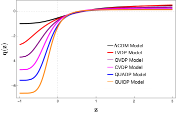
Figure 1: The figure shows the evolution of the deceleration parameter for the considered models resulting from Pacif parametrization scheme. We can interpret the higher acceleration rate for the described models in the late phase of the evolution.

III Methodology

In our analysis, we have chosen a subset of the latest Baryon Acoustic Oscillation (BAO) measurements sourced from various galaxy survey experiments. The predominant contributors to this subset are the Sloan Digital Sky Survey (SDSS) [18, 19, 20, 21, 22, 23]. Additionally, we have incorporated data from the Dark Energy Survey (DES) [24], the Dark Energy Camera Legacy Survey (DECaLS) [25], and 6dFGS BAO [26]. In any our analysis, understanding and properly accounting for correlations within the data are crucial for drawing accurate conclusions. This is especially true in cosmology, where precise measurements of observables like the Baryon Acoustic Oscillations (BAO) are essential for constraining cosmological models. In our analysis, we recognize the potential for correlations among selected data points, which could arise from various sources such as instrumental effects, observational biases, or underlying physical processes. To address this, we adopt a comprehensive approach outlined in [27], leveraging the concept of covariance matrices. The covariance matrix encapsulates the statistical relationships between different measurements in our dataset. In our case, we aim to estimate the covariance matrix for the BAO data, which informs us about the uncertainties and correlations associated with each measurement. However, accurately determining the covariance matrix is challenging, especially when dealing with diverse measurements from different observational surveys. To tackle this challenge, we employ a methodology inspired by [27]. Firstly, we acknowledge that while we intentionally curate a subset of data to mitigate highly correlated points, intrinsic correlations may still exist within our chosen data points. To simulate these correlations, we introduce non-diagonal elements into the covariance matrix while ensuring symmetry. This process involves randomly selecting pairs of data points and assigning non-diagonal elements with magnitudes determined by the product of the 1$\sigma$ errors of the corresponding data points, scaled by a factor of 0.5. By incorporating these non-diagonal elements, we effectively model correlations between pairs of measurements. It’s worth noting that this approach allows us to represent correlations within approximately 55% of the BAO dataset. While the specific locations of the non-diagonal elements are chosen randomly, the magnitudes are calculated to reflect the expected level of correlation between the corresponding data points. This enables us to more accurately capture the true statistical properties of the dataset and improve the robustness of our analysis. Our analysis employs Polychord, a nested sampling algorithm suitable for high-dimensional parameter spaces, along with the GetDist package for visualizing results [28, 29]. This combination of computational tools ensures efficient exploration of the parameter space and clear presentation of the results. This algorithm facilitates the necessary calculations for our analysis. To determine the best fit values for our cosmological model parameters, we augment the Baryon Acoustic Oscillations (BAO) dataset by incorporating thirty uncorrelated Hubble parameter measurements obtained through the cosmic chronometers (CC) method, detailed in [30, 31, 32, 33]. The latest Pantheon sample data on Type Ia Supernovae [34] is also incorporated. Expanding our observational scope, we introduce 24 binned quasar distance modulus data from [35], a set of 162 Gamma-Ray Bursts (GRBs) as outlined in [36], and the recent Hubble constant measurement (R22) [37] as an additional prior.

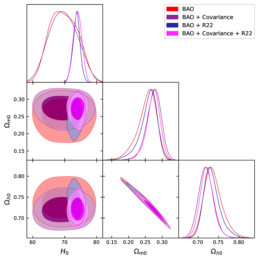
(a) $\Lambda$CDM Model

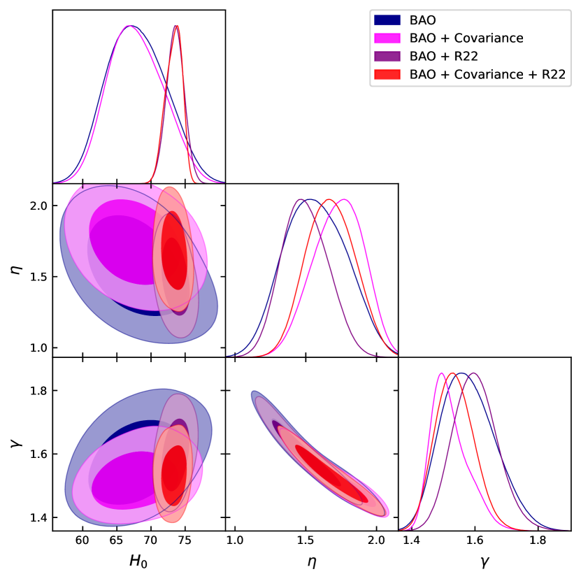
(b) LVDP Model

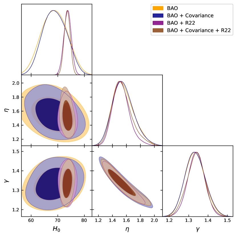
(c) QVDP Model

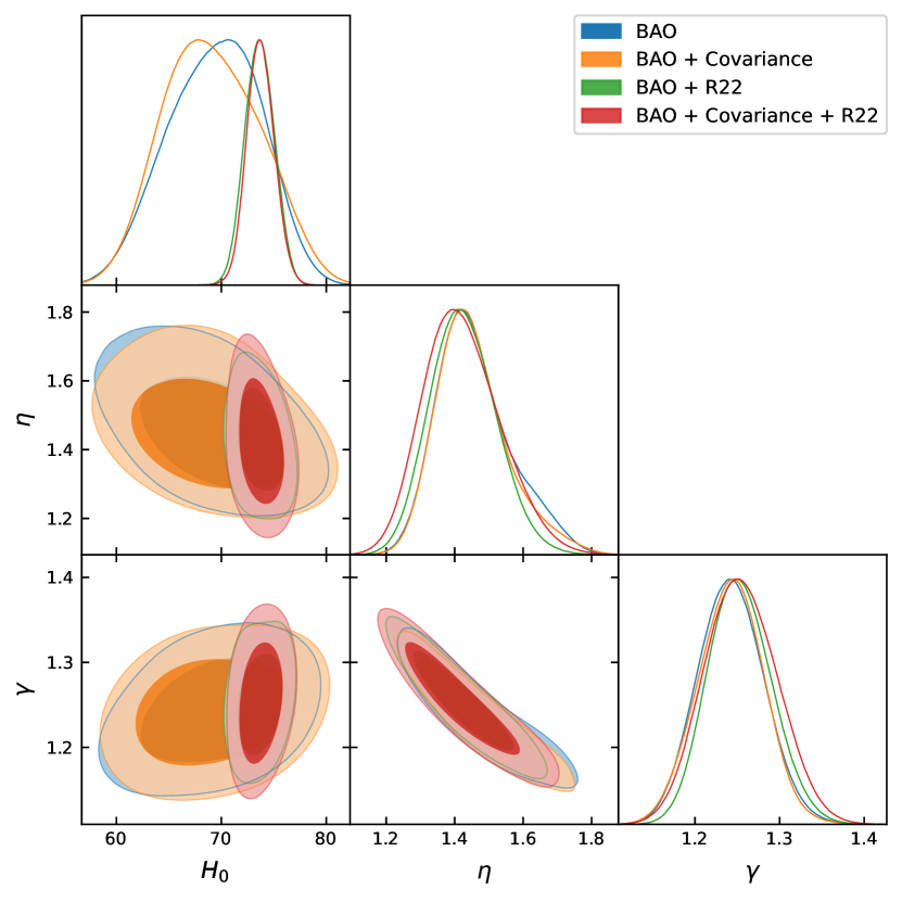
(d) CVDP Model

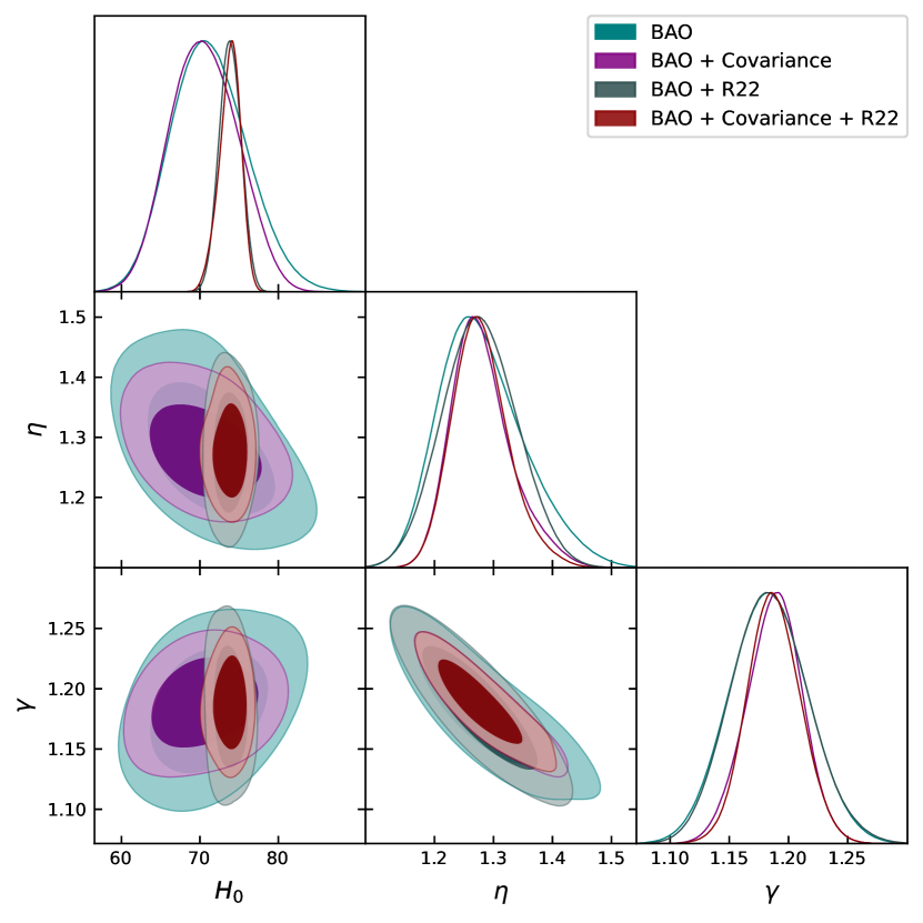
(e) QUADP Model

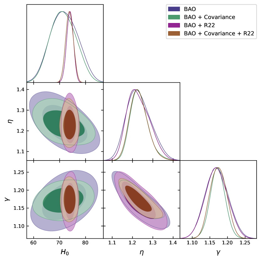
(f) QUIDP Model

Figure 2: The figure illustrates posterior distributions for $\Lambda$CDM, LVDP, QVDP, CVDP, QUADP, and QUIDP models using covariance matrix simulation. The impact of covariance matrices with up to fourteen components is negligible, closely resembling the uncorrelated dataset.

MCMC Results
Model	Parameters	Priors	BAO	BA0 + R22	JOINT	JOINT + R22
	$H_{0}$	[50,100]	$70.256500_{\pm 5.502574}^{\pm 9.206346}$	$73.798696_{\pm 1.315504}^{\pm 2.543240}$	$69.837362_{\pm 1.204873}^{\pm 2.478047}$	$71.508817_{\pm 0.882681}^{\pm 1.614354}$
$\Lambda$CDM Model	$\Omega_{m0}$	[0.,1.]	$0.270161_{\pm 0.013827}^{\pm 0.033280}$	$0.268255_{\pm 0.016790}^{\pm 0.043787}$	$0.274526_{\pm 0.009858}^{\pm 0.021367}$	$0.270609_{\pm 0.009678}^{\pm 0.022243}$
	$\Omega_{\Lambda 0}$	[0.,1.]	$0.725842_{\pm 0.011842}^{\pm 0.019262}$	$0.727203_{\pm 0.013626}^{\pm 0.024379}$	$0.721607_{\pm 0.007421}^{\pm 0.015585}$	$0.724854_{\pm 0.007274}^{\pm 0.016354}$
	$r_{d}$(Mpc)	[100.,200.]	$145.807497_{\pm 9.060325}^{\pm 13.994434}$	$138.345762_{\pm 2.451777}^{\pm 4.939114}$	$145.811932_{\pm 2.347736}^{\pm 4.545176}$	$142.591327_{\pm 1.850175}^{\pm 3.951717}$
	$r_{d}/r_{fid}$	[0.9,1.1]	$0.970661_{\pm 0.055989}^{\pm 0.068973}$	$0.930500_{\pm 0.021272}^{\pm 0.028238}$	$0.974064_{\pm 0.033510}^{\pm 0.057975}$	$0.947662_{\pm 0.028335}^{\pm 0.043021}$
	$H_{0}$	[50,100]	$66.482988_{\pm 4.327756}^{\pm 7.523273}$	$73.399178_{\pm 1.233332}^{\pm 2.121464}$	$69.843835_{\pm 1.201188}^{\pm 2.309027}$	$71.089862_{\pm 1.098795}^{\pm 1.860672}$
	$\eta$	[1.,2.]	$1.543359_{\pm 0.155930}^{\pm 0.235588}$	$1.505127_{\pm 0.135579}^{\pm 0.238943}$	$1.317313_{\pm 0.029436}^{\pm 0.059173}$	$1.306306_{\pm 0.032358}^{\pm 0.057578}$
LVDP Model	$\gamma$	[1.,2.]	$1.569973_{\pm 0.060727}^{\pm 0.091963}$	$1.584289_{\pm 0.049574}^{\pm 0.095406}$	$1.680261_{\pm 0.026752}^{\pm 0.052267}$	$1.686528_{\pm 0.027463}^{\pm 0.059128}$
	$r_{d}$[Mpc]	[100.,200.]	$150.937767_{\pm 10.441640}^{\pm 16.766344}$	$136.635444_{\pm 2.578943}^{\pm 4.733164}$	$145.943266_{\pm 2.304359}^{\pm 4.424778}$	$143.601708_{\pm 2.166555}^{\pm 3.924557}$
	$r_{d}/r_{fid}$	[0.9,1.1]	$0.998261_{\pm 0.061398}^{\pm 0.089931}$	$0.924664_{\pm 0.019297}^{\pm 0.024037}$	$0.973964_{\pm 0.030519}^{\pm 0.056464}$	$0.970574_{\pm 0.040491}^{\pm 0.062762}$
	$H_{0}$	[50,100]	$68.017390_{\pm 5.502190}^{\pm 9.000160}$	$73.595898_{\pm 1.429806}^{\pm 3.369978}$	$70.087223_{\pm 1.264577}^{\pm 2.277802}$	$71.888510_{\pm 0.827500}^{\pm 1.603132}$
	$\eta$	[1.,1.8]	$1.513947_{\pm 0.103619}^{\pm 0.180219}$	$1.479251_{\pm 0.092796}^{\pm 0.174662}$	$1.448643_{\pm 0.029855}^{\pm 0.050227}$	$1.439787_{\pm 0.026722}^{\pm 0.054590}$
QVDP Model	$\gamma$	[1.4,1.9]	$1.335297_{\pm 0.044559}^{\pm 0.069363}$	$1.348510_{\pm 0.042361}^{\pm 0.071797}$	$1.359721_{\pm 0.018284}^{\pm 0.037738}$	$1.362556_{\pm 0.020792}^{\pm 0.035116}$
	$r_{d}$[Mpc]	[100.,200.]	$150.225201_{\pm 11.258422}^{\pm 15.858283}$	$138.891329_{\pm 3.466679}^{\pm 5.163317}$	$146.210595_{\pm 2.671690}^{\pm 5.011410}$	$142.833096_{\pm 1.905742}^{\pm 3.171225}$
	$r_{d}/r_{fid}$	[0.9,1.1]	$0.995485_{\pm 0.075653}^{\pm 0.091697}$	$0.930051_{\pm 0.022072}^{\pm 0.029993}$	$0.973640_{\pm 0.032980}^{\pm 0.056831}$	$0.952014_{\pm 0.029676}^{\pm 0.049829}$
	$H_{0}$	[50,100]	$69.506692_{\pm 5.350084}^{\pm 8.430425}$	$73.142361_{\pm 1.084264}^{\pm 2.735830}$	$70.088663_{\pm 1.290002}^{\pm 2.347399}$	$71.911324_{\pm 0.855184}^{\pm 1.579444}$
	$\eta$	[1.,1.6]	$1.382735_{\pm 0.069212}^{\pm 0.118744}$	$1.375000_{\pm 0.059582}^{\pm 0.102037}$	$1.407113_{\pm 0.023459}^{\pm 0.040118}$	$1.401784_{\pm 0.020468}^{\pm 0.036233}$
CVDP Model	$\gamma$	[1.,2.]	$1.259448_{\pm 0.032302}^{\pm 0.060567}$	$1.262592_{\pm 0.029561}^{\pm 0.050216}$	$1.247435_{\pm 0.018592}^{\pm 0.034410}$	$1.247799_{\pm 0.015954}^{\pm 0.030613}$
	$r_{d}$[Mpc]	[100.,200.]	$149.861013_{\pm 11.055284}^{\pm 15.937774}$	$142.044018_{\pm 3.263304}^{\pm 6.072791}$	$146.722702_{\pm 2.920468}^{\pm 5.262417}$	$143.240618_{\pm 1.733483}^{\pm 3.419517}$
	$r_{d}/r_{fid}$	[0.9,1.1]	$0.992710_{\pm 0.068800}^{\pm 0.087398}$	$0.942123_{\pm 0.025720}^{\pm 0.038254}$	$0.973512_{\pm 0.028596}^{\pm 0.062725}$	$0.952935_{\pm 0.026496}^{\pm 0.048923}$
	$H_{0}$	[50,100]	$71.809820_{\pm 4.373745}^{\pm 7.774584}$	$73.903316_{\pm 1.204603}^{\pm 2.419905}$	$70.257645_{\pm 1.023036}^{\pm 1.834241}$	$71.716330_{\pm 0.867129}^{\pm 1.404752}$
	$\eta$	[1.,1.45]	$1.229965_{\pm 0.036009}^{\pm 0.064755}$	$1.229999_{\pm 0.035752}^{\pm 0.063632}$	$1.310605_{\pm 0.012969}^{\pm 0.024020}$	$1.308932_{\pm 0.014236}^{\pm 0.024276}$
QUADP Model	$\gamma$	[1.,1.5]	$1.194822_{\pm 0.026183}^{\pm 0.044178}$	$1.195622_{\pm 0.024914}^{\pm 0.047978}$	$1.149519_{\pm 0.013532}^{\pm 0.024631}$	$1.148606_{\pm 0.012843}^{\pm 0.027587}$
	$r_{d}$ (Mpc)	[100.,200.]	$150.404609_{\pm 9.337908}^{\pm 15.311542}$	$145.723023_{\pm 4.129844}^{\pm 8.062817}$	$147.192723_{\pm 2.253185}^{\pm 4.304390}$	$144.383543_{\pm 1.707414}^{\pm 3.597572}$
	$r_{d}/r_{fid}$	[0.9,1.1]	$1.000381_{\pm 0.061289}^{\pm 0.093399}$	$0.971004_{\pm 0.038951}^{\pm 0.068012}$	$0.973616_{\pm 0.031554}^{\pm 0.053939}$	$0.956256_{\pm 0.025992}^{\pm 0.046529}$
	$H_{0}$	[50,100]	$72.717604_{\pm 4.717953}^{\pm 8.174180}$	$74.018751_{\pm 1.370823}^{\pm 2.524043}$	$70.420395_{\pm 1.243293}^{\pm 2.148247}$	$72.049908_{\pm 0.838859}^{\pm 1.519503}$
	$\eta$	[1.,1.4]	$1.182361_{\pm 0.033368}^{\pm 0.059293}$	$1.184571_{\pm 0.034052}^{\pm 0.056818}$	$1.274757_{\pm 0.011483}^{\pm 0.022650}$	$1.273832_{\pm 0.011849}^{\pm 0.021953}$
QUIDP Model	$\gamma$	[1.,1.5]	$1.182133_{\pm 0.023581}^{\pm 0.046609}$	$1.181583_{\pm 0.025248}^{\pm 0.044478}$	$1.122719_{\pm 0.013077}^{\pm 0.029113}$	$1.120737_{\pm 0.014876}^{\pm 0.027763}$
	$r_{d}$ (Mpc)	[100.,200.]	$151.765247_{\pm 9.674991}^{\pm 15.340387}$	$148.365470_{\pm 4.899820}^{\pm 9.457728}$	$147.185037_{\pm 2.348354}^{\pm 4.439824}$	$144.031174_{\pm 1.604601}^{\pm 3.256083}$
	$r_{d}/r_{fid}$	[0.9,1.1]	$1.001306_{\pm 0.059456}^{\pm 0.093722}$	$0.983450_{\pm 0.042492}^{\pm 0.074993}$	$0.975632_{\pm 0.030775}^{\pm 0.062454}$	$0.951285_{\pm 0.028220}^{\pm 0.045721}$

Table 1: Constraints at 95% CL on the cosmological parameters for $\Lambda$CDM, LVDP, QVDP, CVDP, QUADP and QUIDP Models

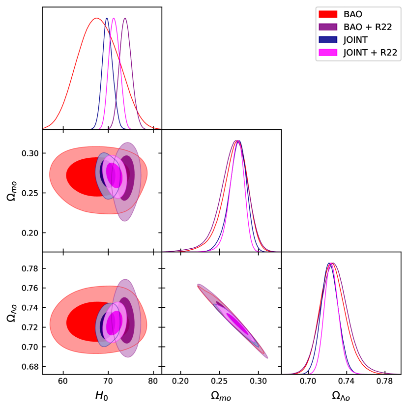
(a) $\Lambda$CDM Model

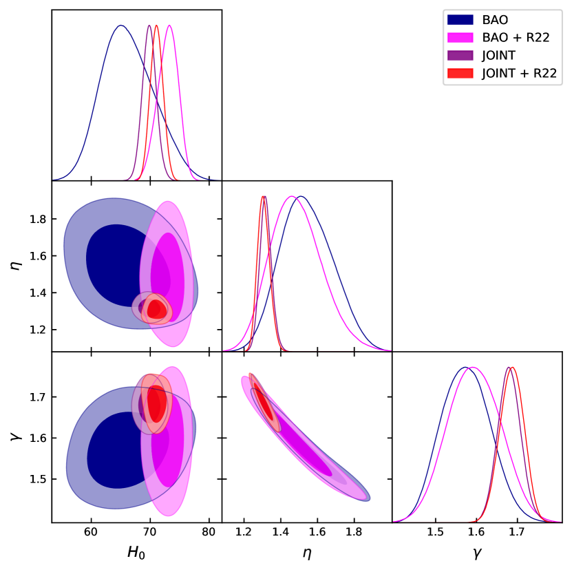
(b) LVDP Model

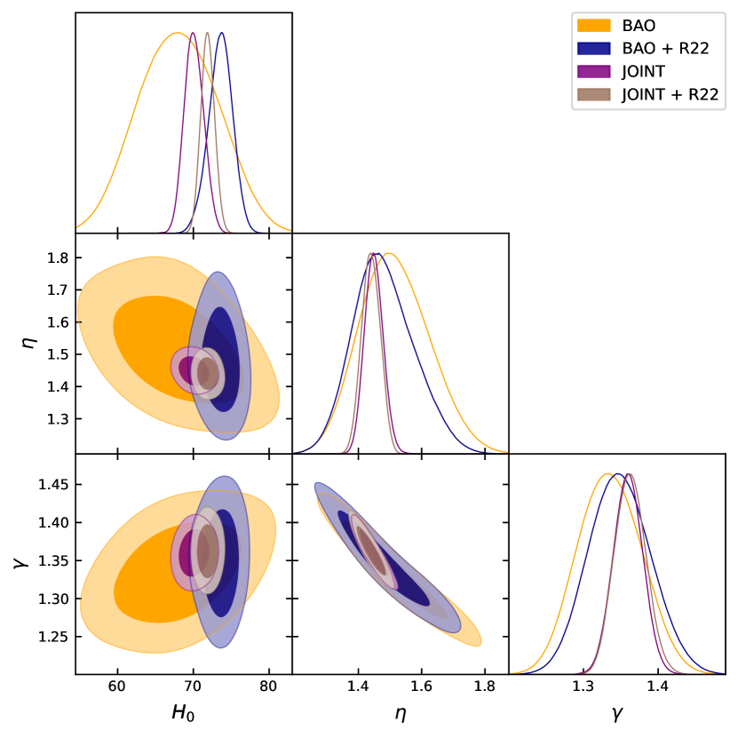
(c) QVDP Model

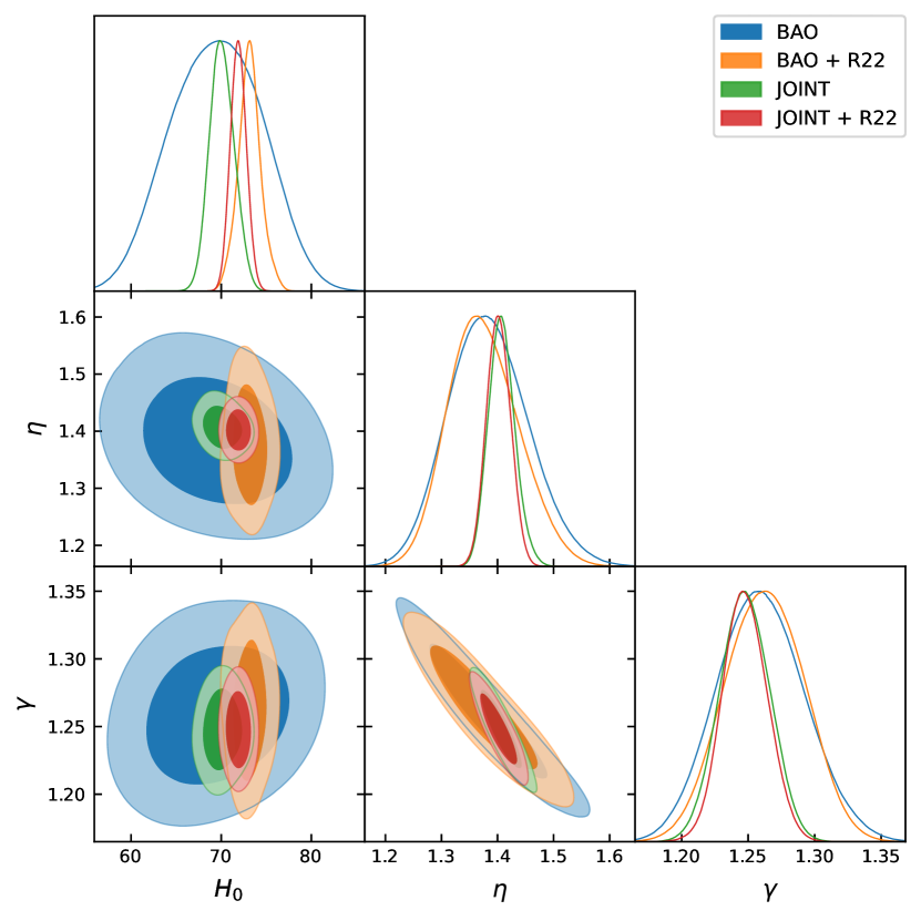
(d) CVDP Model

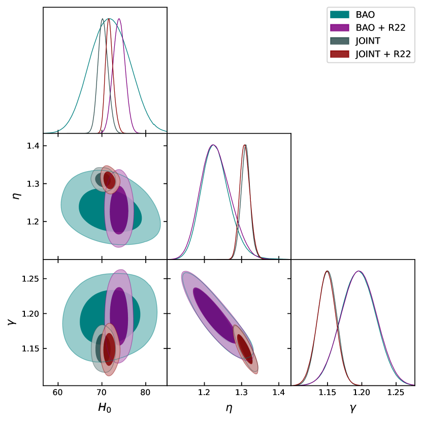
(e) QUADP Model

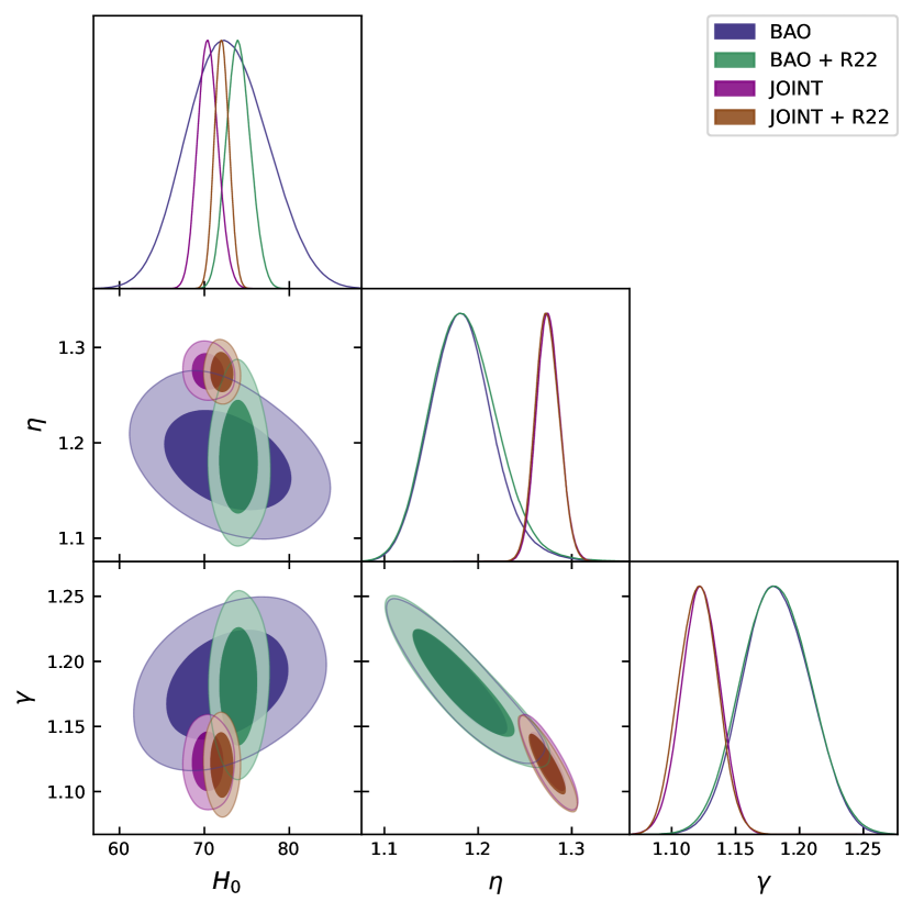
(f) QUIDP Model

Figure 3: The figure presents the posterior distribution for various observational data measurements with the $\Lambda$CDM, LVDP, QVDP, CVDP, QUADP and QUIDP Models indicating 1 $\sigma$ and 2$\sigma$ confidence intervals.

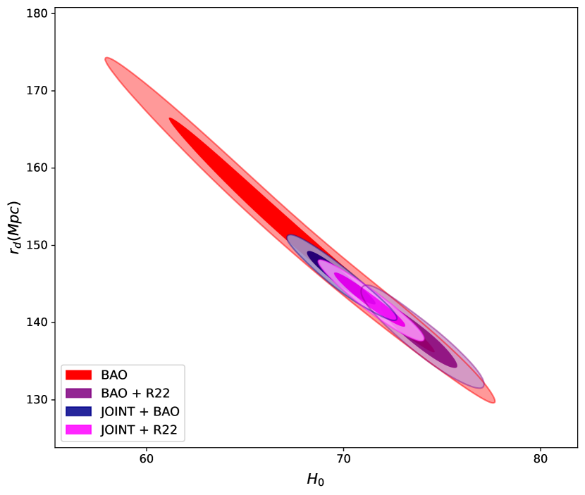
(a) $\Lambda$CDM Model

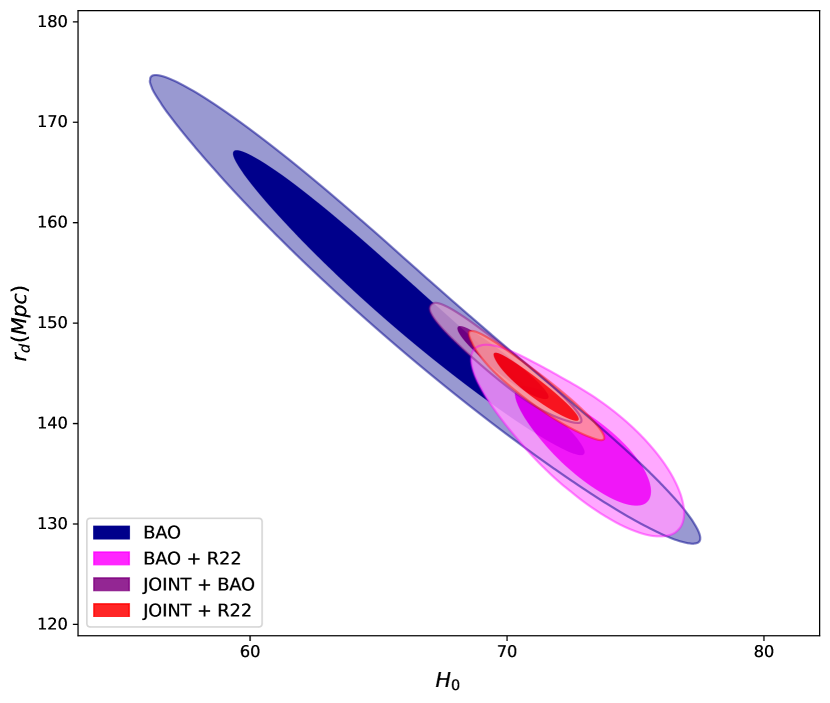
(b) LVDP Model

(c) QVDP Model

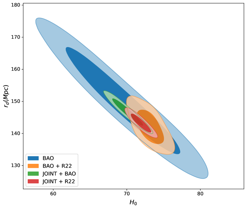
(d) CVDP Model

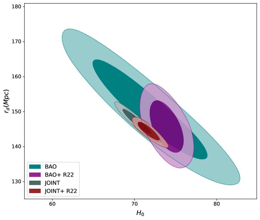
(e) QUADP Model

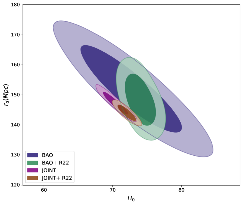
(f) QUIDP Model

Figure 4: The figure displays the posterior distribution for various observational data measurements in the $r_{d}$ vs $H_{0}$ contour plane of the $\Lambda$CDM, LVDP, QVDP, CVDP, QUADP and QUIDP Models, indicating 1 $\sigma$ and 2$\sigma$ confidence intervals.

IV Results

The Fig 1 provides valuable insights into the behavior of the late Universe utilizing the Pacif Parametrization Scheme, which yields cosmological models featuring deceleration parameters of varying orders with respect to cosmic time $t$. Notably, these models exhibit a compelling cosmological phase transition from an early decelerating phase to a late accelerating phase. The LVDP, QVDP, CVDP, QUADP, and QUIDP models all demonstrate this characteristic transition, eventually entering a phase of super acceleration ($q<-1$) in the distant future. This implication suggests that in these models, the universe will undergo a ”Big Rip” scenario, culminating in a singularity and the disintegration of all bound structures, including galaxies, stars, and even atoms. Consequently, Fig 2 illustrates posterior distributions for six cosmological models ($\Lambda$CDM, LVDP, QVDP, CVDP, QAVDP, and QIVDP) with and without the inclusion of a test random covariance matrix comprising fourteen components. Surprisingly, varying from null to fourteen components, the covariance matrix has minimal impact, closely resembling the uncorrelated dataset. These findings suggest limited influence on model posterior distributions. Additionally, despite efforts to minimize correlations within our selected data subset, intrinsic correlations may persist. To simulate such correlations, we introduce non-diagonal elements into the covariance matrix, maintaining symmetry. These elements are randomly assigned with magnitudes based on the product of corresponding data point errors, scaled by 0.5, effectively covering about 55% of the BAO dataset. While non-diagonal elements’ positions are random, their magnitudes reflect expected correlations, enhancing dataset representation. Fig 2(a), 2(b), 2(c), 2(d), 2(e), and 2(f) display posterior distributions for $\Lambda$CDM, LVDP, QVDP, CVDP, QAVDP, and QIVDP respectivel, with and without a test random covariance matrix of fourteen components. These findings suggest limited influence on model posterior distributions. In Figs. 3(a), 3(b), 3(c), 3(d), 3(e), and 3(f), the $68\%$ and $95\%$ confidence levels depict the posterior distribution of key cosmological parameters in the $\Lambda$CDM, LVDP, QVDP, CVDP, QUADP, and QUIDP models. The optimal values of each model are represented in Table 1. By observing the $H_{0}$ values presented in Table 1 for each model, one can notice that when the R22 prior is incorporated into the Joint dataset, the optimal fitting value for $H_{0}$ deviates from the result in [38] but closely aligns with measurements from the SNIe sample in [37]. In the absence of R22 priors with the Joint dataset, the estimated $H_{0}$ aligns more closely with the value obtained in [38] in each model. For the Standard $\Lambda$CDM model, the determined values for the matter density, referred to as $\Omega_{m0}$, and the dark energy density, represented by $\Omega_{\Lambda 0}$, seem to be relatively lower compared to the documented values in [38]. In the context of the Baryon Acoustic Oscillations (BAO) scale, it is defined by the cosmic sound horizon imprinted in the cosmic microwave background during the drag epoch, denoted as $z_{d}$. This epoch marks the separation of baryons and photons. The BAO scale, represented by $r_{d}$, is determined by the integral of the ratio of the speed of sound ($c_{s}$) to the Hubble parameter ($H$) over the redshift range from $z_{d}$ to infinity. The speed of sound, $c_{s}$, is given by $\sqrt{\frac{\delta p_{\gamma}}{\delta\rho_{B}+\delta\rho_{\gamma}}}$, where $\delta p_{\gamma}$ is the pressure perturbation in photons, and $\delta\rho_{B}$ and $\delta\rho_{\gamma}$ are perturbations in the baryon and photon energy densities, respectively. This expression is further simplified to $\frac{1}{\sqrt{3(1+R)}}$, with $R$ defined as the ratio of baryon density perturbation to photon density perturbation ($R\equiv\frac{\delta\rho_{B}}{\delta\rho_{\gamma}}=\frac{3\rho_{B}}{4\rho_{\gamma}}$). Observational data from [38] provides the redshift at the drag epoch as $z_{d}=1059.94\pm 0.30$. Fig 4 illustrates the posterior distribution of the contour plane for $r_{d}-H_{0}$ in the $\Lambda$CDM model and each dark energy model obtained from different parameterizations. In Fig 4(a), the BAO datasets estimate $r_{d}$ as $145.807\pm 9.06$ Mpc, consistent with [38]. When R22 prior is included exclusively, $r_{d}$ becomes $138.345\pm 2.45$ Mpc. For the Joint dataset, $r_{d}$ is $145.811\pm 2.34$ Mpc, aligning closely with [38]. Incorporating R22 into the comprehensive dataset results in $r_{d}$ of $142.591\pm 1.49$ Mpc, similar to [39]. Transitioning to the LVDP parameterization, Fig 4(b) showcases the contour plane of $r_{d}-H_{0}$. In the case of BAO datasets, $r_{d}$ is $150.225\pm 11.258$ Mpc. When exclusively incorporating the R22 prior into BAO datasets, the sound horizon at the drag epoch is $138.891\pm 3.466$ Mpc. For the Joint dataset, $r_{d}$ is $145.943\pm 2.30$ Mpc, closely resembling [38]. Integrating the R22 prior into the comprehensive dataset yields $r_{d}=143.601\pm 2.166$ Mpc, akin to the results in [39]. Moving to the QVDP parameterization (Fig 4(c)), the contour plane of $r_{d}-H_{0}$ is depicted. BAO datasets estimate $r_{d}$ as $150.225\pm 11.258$ Mpc. Introducing the R22 prior into BAO datasets results in a sound horizon of $138.891\pm 3.466$ Mpc. For the Joint dataset, $r_{d}$ is $146.210\pm 2.671$ Mpc, resembling [38]. Incorporating the R22 prior into the complete dataset yields $r_{d}=142.833\pm 1.905$ Mpc, in agreement with [39]. Shifting our focus to the CVDP parameterization Fig 4(d), the contour plane of $r_{d}-H_{0}$ is illustrated. BAO datasets estimate $r_{d}$ as $149.861\pm 11.055$ Mpc. Introducing the R22 prior into BAO datasets alone results in a sound horizon of $142.044\pm 3.263$ Mpc. For the Joint dataset, $r_{d}$ is $146.722\pm 2.920$ Mpc, aligning with [38]. Incorporating the R22 prior into the full dataset yields $r_{d}=143.240\pm 1.733$ Mpc, showing proximity to the outcomes in [39]. Turning our attention to the QUADP parameterization Fig 4(e), the contour plane of $r_{d}-H_{0}$ is shown. BAO datasets estimate $r_{d}$ as $150.404\pm 9.377$ Mpc. Introducing the R22 prior into BAO datasets alone yields a sound horizon of $145.723\pm 4.129$ Mpc. For the Joint dataset, $r_{d}$ is $147.192\pm 2.253$ Mpc, closely resembling [38]. Incorporating the R22 prior into the full dataset results in $r_{d}=144.383\pm 1.707$ Mpc, showing proximity to the outcomes in [39]. Finally Shifting focus to the QUIDP parameterization Fig 4(f), the contour plane of $r_{d}-H_{0}$ is depicted. BAO datasets estimate $r_{d}$ as $151.765\pm 9.674$ Mpc. Introducing the R22 prior into BAO datasets alone yields a sound horizon of $148.365\pm 4.899$ Mpc. For the Joint dataset, $r_{d}$ is $147.185\pm 2.348$ Mpc, closely resembling [38]. Incorporating the R22 prior into the full dataset results in $r_{d}=144.031\pm 1.604$ Mpc, showing proximity to the outcomes in [39]. The $r_{d}$ values obtained from the joint dataset in the $\Lambda$CDM, LVDP, QVDP, CVDP, QUADP, and QUIDP models exhibit close agreement with the estimates provided by Planck and SDSS. [40] reports that by employing Binning and Gaussian methods to combine measurements of 2D BAO and SNIa data, the values of the absolute $\mathrm{BAO}$ scale range from 141.45 Mpc to $r_{d}\leq 159.44\mathrm{Mpc}$ (Binning) and 143.35 Mpc to $r_{d}\leq 161.59\mathrm{Mpc}$ (Gaussian). These findings highlight a clear discrepancy between early and late-time observational measurements, analogous to the $H_{0}$ tension. It is noteworthy that our results are contingent on the range of priors for $r_{d}$ and $H_{0}$, influencing the estimated values in the $r_{d}-H_{0}$ contour plane. In our quest to compare various cosmological models, we employ two widely used criteria, namely the Akaike Information Criterion (AIC) [41] and the Bayesian Information Criterion (BIC) [42]. The AIC is given by the formula: $\text{AIC}=-2\ln(\mathcal{L}_{\text{max}})+2k+\frac{2k(2k+1)}{N_{\text{tot}}-k-1}$ Here, $\mathcal{L}_{\text{max}}$ represents the maximum likelihood of the data, $N_{\text{tot}}$ is the total number of data points (in our case, $N_{\text{tot}}=299$), and $k$ is the number of parameters. For sufficiently large $N_{\text{tot}}$, the expression simplifies to the standard form: $\text{AIC}\approx-2\ln(\mathcal{L}_{\text{max}})+2k$. The Bayesian Information Criterion is defined as $\text{BIC}=-2\ln(\mathcal{L}_{\text{max}})+k\ln(N_{\text{tot}})$ By applying these criteria to the standard $\Lambda$CDM, LVDP, QVDP, CVDP, QUADP and QUIDP models, we obtain AIC values of [264.53, 275.62, 271.48, 271.08, 274.66, 278.72] and BIC values of [264.53, 275.85, 271.71, 271.30, 274.88, 278.94] for the respective models. While the $\Lambda$CDM model exhibits the best fit due to the lowest AIC, it is noteworthy that our AIC and BIC values collectively lend substantial support to all the tested models. Consequently, none of the models can be conclusively ruled out based on the current dataset. This underscores the robustness of our findings and the validity of the cosmological models under consideration. When comparing the LVDP, QVDP, CVDP, QUADP and QUIDP models to $\Lambda$CDM, it is important to note that $\Lambda$CDM is nested within both proposed extensions, with a difference of 5 degrees of freedom. This characteristic enables the application of standard statistical tests. The assessment involves utilizing the reduced chi-square statistic, denoted as $\chi_{\text{red}}^{2}=\chi^{2}/\text{Dof}$, where Dof represents the degrees of freedom of the model, and $\chi^{2}$ signifies the weighted sum of squared deviations. Under an equal number of runs for the three models, the reduced chi-square statistic closely approximates 1, as shown by the values: $\left(\frac{\chi^{2}}{Dof_{\Lambda CDM}},\frac{\chi^{2}}{Dof_{LVDP}},\frac{\chi^{2}}{Dof_{QVDP}},\frac{\chi^{2}}{Dof_{CVDP}},\frac{\chi^{2}}{Dof_{QUADP}},\frac{\chi^{2}}{Dof_{QUIDP}}\right)\approx\{0.961646,0.955499,0.943959,0.955646,0.952016,0.966625\}$. This comparative analysis provides insights into the goodness of fit for each model, where values close to 1 suggest a reasonable fit to the data.

V Conclusion

In our investigation, we adopt a parametrization scheme for the Hubble parameter, yielding diverse cosmological models with varying deceleration parameter profiles. These models, including LVDP, QVDP, CVDP, QUADP, and QUIDP, exhibit distinct behaviors in the late-time evolution of the Universe. By constraining model parameters, such as $\eta$ and $\gamma$, we aim to align these models with observational data. The parametrization approach offers a versatile framework for exploring the cosmic dynamics, shedding light on the Universe’s expansion history and its transition to an accelerating phase. Through the analysis of the deceleration parameter as functions of redshift, we gain valuable insights into the cosmological implications of different orders of deceleration parameter functions, providing a comprehensive understanding of the late-time evolution of the Universe. Furthermore, we have meticulously selected 24 Baryon Acoustic Oscillation (BAO) data points from a large dataset of 333 BAO points, ensuring their independence and reliability for our analysis. The objective behind this selection is to minimize intrinsic errors in the posterior distribution that might result from possible correlations among measurements. A specific procedure was implemented to simulate the introduction of random correlations to the covariance matrix. Subsequent verification confirmed that these simulated additions do not lead to noteworthy changes in the cosmological parameters derived from the study. Additionally, alongside the BAO data, we incorporated low-redshift data, including 33 independent Hubble Measurements from Cosmic Chronometers, 40 data points from Type Ia supernovae, 24 points from the Hubble diagram for quasars, and a substantial dataset comprising 162 points from Gamma-Ray Bursts. This comprehensive dataset, along with the most recent Hubble constant measurement by R22, allows us to analyze the sensitivity of the Hubble constant and sound horizon within the Pacif parametrization. Instead of imposing a prior constraint on the sound horizon $r_{d}$ from CMB measurements, we treat $r_{d}$ as a free parameter. We find $H_{0}=69.837362\pm 1.204873\ \mathrm{km/s/Mpc}$ and $r_{d}=145.811932\pm 2.347736\ \mathrm{Mpc}$ in $\Lambda$CDM model, $H_{0}=69.843835\pm 1.201188\ \mathrm{km/s/Mpc}$ and $r_{d}=145.943266\pm 2.304359\ \mathrm{Mpc}$ in LVDP model, $H_{0}=70.087223\pm 1.264577\ \mathrm{km/s/Mpc}$ and $r_{d}=146.210595\pm 2.671690\ \mathrm{Mpc}$ in QVDP model, $H_{0}=70.088663\pm 1.290002\ \mathrm{km/s/Mpc}$ and $r_{d}=146.722702\pm 2.920468\ \mathrm{Mpc}$ in CVDP model, $H_{0}=70.257645\pm 1.023036\ \mathrm{km/s/Mpc}$ and $r_{d}=147.192723\pm 2.253185\ \mathrm{Mpc}$ in QUADP model and $H_{0}=70.420395\pm 1.243293\ \mathrm{km/s/Mpc}$ and $r_{d}=147.185037\pm 2.348354\ \mathrm{Mpc}$ in model. Remarkably, our findings indicate that the $H_{0}$ and $r_{d}$ values derived from low-redshift measurements are consistent with early Planck estimates [38, 43, 44, 40]. The application of both the Akaike Information Criterion (AIC) and the Bayesian Information Criterion (BIC) to various cosmological models reveals valuable insights into their comparative performance. Despite the $\Lambda$CDM model exhibiting the best fit according to the lowest AIC value, all tested models receive substantial support from the AIC and BIC values, indicating their validity. Consequently, none of the models can be definitively ruled out based on the current dataset, underscoring the robustness of our findings. Furthermore, when comparing the LVDP, QVDP, CVDP, QUADP, and QUIDP models to $\Lambda$CDM, it’s crucial to note that $\Lambda$CDM is nested within both proposed extensions, differing by no degrees of freedom. This nesting allows for standard statistical tests, as evidenced by the reduced chi-square statistics closely approximating 1 for each model. These findings suggest a reasonable fit to the data for all models considered. Concluding the paper, our investigation into Pacif parametrization models elucidates their efficacy in capturing late-time cosmological evolution and addressing existing tensions. By incorporating non-diagonal elements in the covariance matrix, we refine constraints and unveil the sensitivity of $H_{0}$ and $r_{d}$ within this framework. Embracing a data-driven approach without CMB priors, we leverage diverse datasets spanning various redshifts, culminating in robust $H_{0}$ and $r_{d}$ estimates. Notably, our findings exhibit coherence with Planck CMB results, affirming the viability of Pacif parametrization models. Our comparative analysis underscores the relevance of the obtained models, offering valuable insights for advancing cosmological understanding amidst evolving observational landscapes.

References

- [1] D. H. Weinberg, M. J. Mortonson, D. J. Eisenstein, C. Hirata, A. G. Riess, and E. Rozo, “Observational probes of cosmic acceleration,” Physics reports, vol. 530, no. 2, pp. 87–255, 2013.
- [2] A. G. Riess, A. V. Filippenko, P. Challis, A. Clocchiatti, A. Diercks, P. M. Garnavich, R. L. Gilliland, C. J. Hogan, S. Jha, R. P. Kirshner, et al., “Observational evidence from supernovae for an accelerating universe and a cosmological constant,” The astronomical journal, vol. 116, no. 3, p. 1009, 1998.
- [3] S. Perlmutter and B. P. Schmidt, “Measuring cosmology with supernovae,” Supernovae and Gamma-Ray Bursters, pp. 195–217, 2003.
- [4] A. Iqbal, J. Prasad, T. Souradeep, and M. A. Malik, “Joint planck and wmap assessment of low cmb multipoles,” Journal of Cosmology and Astroparticle Physics, vol. 2015, no. 06, p. 014, 2015.
- [5] C.-H. Chuang, F. Prada, F. Beutler, D. J. Eisenstein, S. Escoffier, S. Ho, J.-P. Kneib, M. Manera, S. E. Nuza, D. J. Schlegel, et al., “The clustering of galaxies in the sdss-iii baryon oscillation spectroscopic survey: single-probe measurements from cmass and lowz anisotropic galaxy clustering,” arXiv preprint arXiv:1312.4889, 2013.
- [6] O. Farooq, F. R. Madiyar, S. Crandall, and B. Ratra, “Hubble parameter measurement constraints on the redshift of the deceleration–acceleration transition, dynamical dark energy, and space curvature,” The Astrophysical Journal, vol. 835, no. 1, p. 26, 2017.
- [7] M. Li, X.-D. Li, S. Wang, and Y. Wang, “Dark energy,” Communications in theoretical physics, vol. 56, no. 3, p. 525, 2011.
- [8] M. Li, X.-D. Li, S. Wang, and Y. Wang, “Dark energy: A brief review,” Frontiers of Physics, vol. 8, pp. 828–846, 2013.
- [9] E. J. Copeland, M. Sami, and S. Tsujikawa, “Dynamics of dark energy,” International Journal of Modern Physics D, vol. 15, no. 11, pp. 1753–1935, 2006.
- [10] B. Kazuharu, S. Capozziello, S. D. Odintsov, et al., “Dark energy cosmology: the equivalent description via different theoretical models and cosmography tests,” ASTROPHYSICS AND SPACE SCIENCE, vol. 342, pp. 155–228, 2012.
- [11] A. Bouali, H. Chaudhary, A. Mehrotra, and S. Pacif, “Model-independent study for a quintessence model of dark energy: Analysis and observational constraints,” arXiv preprint arXiv:2304.02652, 2023.
- [12] S. K. J. Pacif, “Dark energy models from a parametrization of h: a comprehensive analysis and observational constraints,” The European Physical Journal Plus, vol. 135, no. 10, pp. 1–34, 2020.
- [13] M. Khurana, H. Chaudhary, S. Mumtaz, S. Pacif, and G. Mustafa, “Cosmic evolution in f (q, t) gravity: Exploring a higher-order time-dependent function of deceleration parameter with observational constraints,” Physics of the Dark Universe, vol. 43, p. 101408, 2024.
- [14] L. Berezhiani, J. Khoury, and J. Wang, “Universe without dark energy: Cosmic acceleration from dark matter-baryon interactions,” Physical Review D, vol. 95, no. 12, p. 123530, 2017.
- [15] M. K. Sharma, S. K. J. Pacif, G. Yergaliyeva, and K. Yesmakhanova, “The oscillatory universe, phantom crossing and the hubble tension,” Annals of Physics, vol. 454, p. 169345, 2023.
- [16] D. Sofuoğlu, H. Baysal, and R. Tiwari, “Observational constraints on the cubic parametrization of the deceleration parameter in f (r, t) gravity,” The European Physical Journal Plus, vol. 138, no. 6, pp. 1–14, 2023.
- [17] V. Kalsariya and S. K. J. Pacif, “Cosmo-dynamics of dark energy models resulting from a parametrization of in gravity,” arXiv preprint arXiv:2304.09163, 2023.
- [18] A. J. Ross, L. Samushia, C. Howlett, W. J. Percival, A. Burden, and M. Manera, “The clustering of the sdss dr7 main galaxy sample–i. a 4 per cent distance measure at z= 0.15,” Monthly Notices of the Royal Astronomical Society, vol. 449, no. 1, pp. 835–847, 2015.
- [19] S. Alam, M. Ata, S. Bailey, F. Beutler, D. Bizyaev, J. A. Blazek, A. S. Bolton, J. R. Brownstein, A. Burden, C.-H. Chuang, et al., “The clustering of galaxies in the completed sdss-iii baryon oscillation spectroscopic survey: cosmological analysis of the dr12 galaxy sample,” Monthly Notices of the Royal Astronomical Society, vol. 470, no. 3, pp. 2617–2652, 2017.
- [20] H. Gil-Marín, J. E. Bautista, R. Paviot, M. Vargas-Magaña, S. de La Torre, S. Fromenteau, S. Alam, S. Ávila, E. Burtin, C.-H. Chuang, et al., “The completed sdss-iv extended baryon oscillation spectroscopic survey: measurement of the bao and growth rate of structure of the luminous red galaxy sample from the anisotropic power spectrum between redshifts 0.6 and 1.0,” Monthly Notices of the Royal Astronomical Society, vol. 498, no. 2, pp. 2492–2531, 2020.
- [21] A. Raichoor, A. De Mattia, A. J. Ross, C. Zhao, S. Alam, S. Avila, J. Bautista, J. Brinkmann, J. R. Brownstein, E. Burtin, et al., “The completed sdss-iv extended baryon oscillation spectroscopic survey: large-scale structure catalogues and measurement of the isotropic bao between redshift 0.6 and 1.1 for the emission line galaxy sample,” Monthly Notices of the Royal Astronomical Society, vol. 500, no. 3, pp. 3254–3274, 2021.
- [22] J. Hou, A. G. Sánchez, A. J. Ross, A. Smith, R. Neveux, J. Bautista, E. Burtin, C. Zhao, R. Scoccimarro, K. S. Dawson, et al., “The completed sdss-iv extended baryon oscillation spectroscopic survey: Bao and rsd measurements from anisotropic clustering analysis of the quasar sample in configuration space between redshift 0.8 and 2.2,” Monthly Notices of the Royal Astronomical Society, vol. 500, no. 1, pp. 1201–1221, 2021.
- [23] H. D. M. Des Bourboux, J. Rich, A. Font-Ribera, V. de Sainte Agathe, J. Farr, T. Etourneau, J.-M. Le Goff, A. Cuceu, C. Balland, J. E. Bautista, et al., “The completed sdss-iv extended baryon oscillation spectroscopic survey: baryon acoustic oscillations with ly forests,” The Astrophysical Journal, vol. 901, no. 2, p. 153, 2020.
- [24] T. Abbott, M. Aguena, S. Allam, A. Amon, F. Andrade-Oliveira, J. Asorey, S. Avila, G. Bernstein, E. Bertin, A. Brandao-Souza, et al., “Dark energy survey year 3 results: A 2.7% measurement of baryon acoustic oscillation distance scale at redshift 0.835,” Physical Review D, vol. 105, no. 4, p. 043512, 2022.
- [25] S. Sridhar, Y.-S. Song, A. J. Ross, R. Zhou, J. A. Newman, C.-H. Chuang, R. Blum, E. Gaztanaga, M. Landriau, and F. Prada, “Clustering of lrgs in the decals dr8 footprint: Distance constraints from baryon acoustic oscillations using photometric redshifts,” The Astrophysical Journal, vol. 904, no. 1, p. 69, 2020.
- [26] F. Beutler, C. Blake, M. Colless, D. H. Jones, L. Staveley-Smith, L. Campbell, Q. Parker, W. Saunders, and F. Watson, “The 6df galaxy survey: baryon acoustic oscillations and the local hubble constant,” Monthly Notices of the Royal Astronomical Society, vol. 416, no. 4, pp. 3017–3032, 2011.
- [27] L. Kazantzidis and L. Perivolaropoulos, “Evolution of the f 8 tension with the planck 15/cdm determination and implications for modified gravity theories,” Physical Review D, vol. 97, no. 10, p. 103503, 2018.
- [28] W. Handley, M. Hobson, and A. Lasenby, “Polychord: nested sampling for cosmology,” Monthly Notices of the Royal Astronomical Society: Letters, vol. 450, no. 1, pp. L61–L65, 2015.
- [29] A. Lewis, “Getdist: a python package for analysing monte carlo samples,” arXiv preprint arXiv:1910.13970, 2019.
- [30] M. Moresco, “Raising the bar: new constraints on the hubble parameter with cosmic chronometers at z 2,” Monthly Notices of the Royal Astronomical Society: Letters, vol. 450, no. 1, pp. L16–L20, 2015.
- [31] M. Moresco, L. Pozzetti, A. Cimatti, R. Jimenez, C. Maraston, L. Verde, D. Thomas, A. Citro, R. Tojeiro, and D. Wilkinson, “A 6% measurement of the hubble parameter at z 0.45: direct evidence of the epoch of cosmic re-acceleration,” Journal of Cosmology and Astroparticle Physics, vol. 2016, no. 05, pp. 014–014, 2016.
- [32] M. Moresco, L. Verde, L. Pozzetti, R. Jimenez, and A. Cimatti, “New constraints on cosmological parameters and neutrino properties using the expansion rate of the universe to z 1.75,” Journal of Cosmology and Astroparticle Physics, vol. 2012, no. 07, p. 053, 2012.
- [33] M. Moresco, A. Cimatti, R. Jimenez, L. Pozzetti, G. Zamorani, M. Bolzonella, J. Dunlop, F. Lamareille, M. Mignoli, H. Pearce, et al., “Improved constraints on the expansion rate of the universe up to z 1.1 from the spectroscopic evolution of cosmic chronometers,” Journal of Cosmology and Astroparticle Physics, vol. 2012, no. 08, pp. 006–006, 2012.
- [34] D. M. Scolnic, D. Jones, A. Rest, Y. Pan, R. Chornock, R. Foley, M. Huber, R. Kessler, G. Narayan, A. Riess, et al., “The complete light-curve sample of spectroscopically confirmed sne ia from pan-starrs1 and cosmological constraints from the combined pantheon sample,” The Astrophysical Journal, vol. 859, no. 2, p. 101, 2018.
- [35] C. Roberts, K. Horne, A. O. Hodson, and A. D. Leggat, “Tests of cdm and conformal gravity using grb and quasars as standard candles out to ,” arXiv preprint arXiv:1711.10369, 2017.
- [36] M. Demianski, E. Piedipalumbo, D. Sawant, and L. Amati, “Cosmology with gamma-ray bursts-ii. cosmography challenges and cosmological scenarios for the accelerated universe,” Astronomy & Astrophysics, vol. 598, p. A113, 2017.
- [37] A. G. Riess, W. Yuan, L. M. Macri, D. Scolnic, D. Brout, S. Casertano, D. O. Jones, Y. Murakami, G. S. Anand, L. Breuval, et al., “A comprehensive measurement of the local value of the hubble constant with 1 km s- 1 mpc- 1 uncertainty from the hubble space telescope and the sh0es team,” The Astrophysical journal letters, vol. 934, no. 1, p. L7, 2022.
- [38] P. Collaboration, N. Aghanim, Y. Akrami, M. Ashdown, J. Aumont, C. Baccigalupi, M. Ballardini, A. Banday, R. Barreiro, N. Bartolo, et al., “Planck 2018 results. vi. cosmological parameters,” 2020.
- [39] L. Verde, J. L. Bernal, A. F. Heavens, and R. Jimenez, “The length of the low-redshift standard ruler,” Monthly Notices of the Royal Astronomical Society, vol. 467, no. 1, pp. 731–736, 2017.
- [40] T. Lemos, Ruchika, J. C. Carvalho, and J. Alcaniz, “Low-redshift estimates of the absolute scale of baryon acoustic oscillations,” The European Physical Journal C, vol. 83, no. 6, p. 495, 2023.
- [41] H. Akaike, “A new look at the statistical model identification,” IEEE transactions on automatic control, vol. 19, no. 6, pp. 716–723, 1974.
- [42] G. Schwarz, “Estimating the dimension of a model,” The annals of statistics, pp. 461–464, 1978.
- [43] R. C. Nunes, S. K. Yadav, J. Jesus, and A. Bernui, “Cosmological parameter analyses using transversal bao data,” Monthly Notices of the Royal Astronomical Society, vol. 497, no. 2, pp. 2133–2141, 2020.
- [44] R. C. Nunes and A. Bernui, “Bao signatures in the 2-point angular correlations and the hubble tension,” The European Physical Journal C, vol. 80, pp. 1–8, 2020.