Generative Modeling for Tabular Data via
Penalized Optimal Transport Network

Abstract

The task of precisely learning the probability distribution of rows within tabular data and producing authentic synthetic samples is both crucial and non-trivial. Wasserstein generative adversarial network (WGAN) marks a notable improvement in generative modeling, addressing the challenges faced by its predecessor, generative adversarial network. However, due to the mixed data types and multimodalities prevalent in tabular data, the delicate equilibrium between the generator and discriminator, as well as the inherent instability of Wasserstein distance in high dimensions, WGAN often fails to produce high-fidelity samples. To this end, we propose POTNet (Penalized Optimal Transport Network), a generative deep neural network based on a novel, robust, and interpretable marginally-penalized Wasserstein (MPW) loss. POTNet can effectively model tabular data containing both categorical and continuous features. Moreover, it offers the flexibility to condition on a subset of features. We provide theoretical justifications for the motivation behind the MPW loss. We also demonstrate empirically the effectiveness of our proposed method on four different benchmarks across a variety of real-world and simulated datasets. Our proposed model achieves orders of magnitude speedup during the sampling stage compared to state-of-the-art generative model for tabular data, thereby enabling efficient large-scale synthetic data generation.

March 5, 2024

Keywords: Generative Models, Synthetic Data Generation, Wasserstein Distance,

Marginal Penalization, Tabular Data Modeling, Deep Learning

1 Introduction

The generation of high-quality tabular data holds significant importance across various domains, particularly in contexts such as medical records (Che et al., 2017; Ghassemi et al., 2020; Zhang et al., 2022), causal discovery (Cinquini et al., 2021), and Bayesian likelihood-free inference (Papamakarios et al., 2019). In the recent years, generative models have achieved tremendous success in a wide range of domains for their ability to learn and generate samples from complex distributions. The promise of such models has spurred the development of generative adversarial networks (GANs) for tabular data generation. GANs, introduced in (Goodfellow et al., 2014), provide greater flexibility in modeling distributions compared to traditional statistical models. To overcome the training instabilities such as vanishing gradients in GANs, Arjovsky et al. proposed Wasserstein GAN (WGAN) which replaces the Jensen-Shannon divergence (JSD) with the $1$-Wasserstein distance (Arjovsky et al., 2017). Their approach leverages the Kantorovich-Rubinstein duality to approximate the Wasserstein distance through a critic network, resulting in a saddle-point objective akin to that of the original GAN framework. Nonetheless, optimizing this saddle-point objective remains challenging, making the training process of WGANs difficult, as highlighted in (Arjovsky and Bottou, 2017; Gulrajani et al., 2017). Particularly in higher dimensions, the estimation of Wasserstein distance is hard due to the curse of dimensionality and its intrinsic flexibility (Fournier and Guillin, 2015; Weed and Bach, 2019). Furthermore, tabular data frequently exhibits multimodality and encompasses mixed data types, comprising both categorical and continuous features. These complex structures present distinct challenges to GANs and WGANs, models initially designed for data with homogeneous feature types like images and text (Borisov et al., 2022b).

In this work, we propose POTNet (Penalized Optimal Transport Network), a generative model for tabular data distributions based on a marginally-penalized Wasserstein (MPW) loss. As opposed to using the Kantorovich-Rubinstein duality, our primal-based method enables direct evaluation of the MPW loss via a single minimization step. This formulation eliminates the need for a discriminator network. Furthermore, our MPW loss is a robust variant of the Wasserstein distance and naturally accommodates mixed data types. To simultaneously model categorical and continuous features, we introduce a corresponding generator network that also allows for conditioning on an arbitrary subset of features. Empirically, we demonstrate the effectiveness of POTNet using a variety of simulated and real datasets. POTNet outperforms all baseline methods and requires significantly less time ($\sim$80x faster) during sample generation than the current state-of-the-art generative model for tabular data.

2 Background

In this section, we formally introduce the problem of generative modeling for tabular data distributions. Then we provide a brief overview of the fundamental concepts related to Wasserstein distance that are needed to develop our framework.

2.1 Generative modeling for tabular data distributions

Let the original dataset be a collection of $n$ i.i.d. real observations drawn from an unknown $d$-dimensional distribution $\mathbb{P}_{r}$. This dataset may include only target features, denoted by $\mathcal{T}\coloneqq\{x^{(i)}\}_{i=1}^{n}$, or it may include a collection of conditional features as well as target features, in which case we denote it as $\mathcal{T}_{C}\coloneqq\{(x^{(i)},y^{(i)})\}_{i=1}^{n}$. Synthetic data generation is performed by first training a generative model $G$ on the original data $\mathcal{T}$ (or $\mathcal{T}_{C}$) and subsequently generating synthetic observations $\{x^{s,(j)}\}_{j=1}^{n^{\prime}}$ (for the unconditional case) or $\{(x^{s,(j)},y^{(j)})\}_{j=1}^{n^{\prime}}$ (for the conditional case, here the conditional features are inputted by the user and are not synthetic). We let $\mathcal{T}^{s}$ denote the synthetic dataset. Depending on the downstream task, different metrics will be used to evaluate the quality of $\mathcal{T}^{s}$ (Xu et al., 2019). We will consider two kinds of metrics in our experimental evaluation: dissimilarity-type metric between $\mathcal{T}$ and $\mathcal{T}^{s}$, and performance metric, which assesses the performance of a machine learning model trained on $\mathcal{T}^{s}$ for the objective task (Fonseca and Bacao, 2023).

2.2 Wasserstein distance

Generative modeling relies crucially on a metric that quantifies the sense of “closeness” between two probability distributions. Our generative model is anchored on a metric called the Wasserstein distance, which allows both primal and dual formulations.

2.2.1 Monge-Kantorovich primal formulation of Wasserstein distance

The Wasserstein distance stems from the subject of optimal transport, which describes transport plans with minimum cost that move mass from one distribution to another. Mathematically, we fix two probability distributions $\mu$ and $\nu$ on two Polish spaces $\mathcal{X}$ and $\mathcal{Y}$, respectively, and choose a lower semicontinuous cost function $c:\mathcal{X}\times\mathcal{Y}\rightarrow[0,\infty]$. The Monge-Kantorovich optimal transport problem is the following minimization problem:

$$\inf_{\pi\in\Pi(\mu,\nu)}\int_{\mathcal{X}\times\mathcal{Y}}c(x,y)d\pi(x,y),$$ (2.1)

where $\Pi(\mu,\nu)$ is the set of probability distributions on $\mathcal{X}\times\mathcal{Y}$ with first and second marginals given by $\mu$ and $\nu$, respectively. Kantorovich (Kantorovich, 2006) showed that (2.1) has at least one solution. The minimal value of $\int_{\mathcal{X}\times\mathcal{Y}}c(x,y)d\pi(x,y)$ achieved by this solution is called the optimal transport cost.

Throughout the rest of this paper, we take $\mathcal{X}=\mathcal{Y}$ to be a Borel subset of some Euclidean space $\mathbb{R}^{d}$, and denote by $\|\cdot\|$ the Euclidean norm on $\mathbb{R}^{d}$. For any $p\geq 1$, we denote by $\mathcal{P}_{p}(\mathcal{X})$ the set of probability distributions on $\mathcal{X}$ with finite $p$th moment (that is, probability distributions $\mu$ with $\int_{\mathcal{X}}\|x\|^{p}d\mu(x)<\infty$). Taking the cost function to be $c(x,y)=\|x-y\|^{p}$, the $p$-Wasserstein distance between $\mu,\nu\in\mathcal{P}_{p}(\mathcal{X})$ is defined as the optimal transport cost for (2.1) raised to the power of $1/p$:

$$W_{p}(\mu,\nu):=\inf_{\pi\in\Pi(\mu,\nu)}\Big{(}\int_{\mathcal{X}\times\mathcal{X}}\|x-y\|^{p}d\pi(x,y)\Big{)}^{1/p}.$$ (2.2)

It can be shown that $W_{p}$ gives a valid metric on $\mathcal{P}_{p}(\mathcal{X})$.

2.2.2 Dual formulation of Wasserstein distance

The $p$-Wasserstein distance as defined in (2.2) also allows the following dual formulation (see e.g. Theorem 5.10 of (Villani et al., 2009)): for any $\mu,\nu\in\mathcal{P}_{p}(\mathcal{X})$,

$$W_{p}(\mu,\nu)=\sup_{\mathcal{F}}\Big{(}\int_{\mathcal{X}}\phi(y)d\nu(y)-\int_{\mathcal{X}}\psi(x)d\mu(x)\Big{)}^{1/p},$$ (2.3)

where $\mathcal{F}$ is the set of pairs of bounded continuous functions $(\psi,\phi)$ on $\mathcal{X}$ that satisfy $\phi(y)-\psi(x)\leq\|x-y\|^{p}$ for all $x,y\in\mathcal{X}$. From Kantorovich-Rubinstein duality (see e.g. Case 5.16 of (Villani et al., 2009)), when $p=1$, (2.3) can be equivalently expressed as

$$W_{1}(\mu,\nu)=\sup_{\|f\|_{Lip}\leq 1}\Big{\{}\int_{\mathcal{X}}fd\mu-\int_{\mathcal{X}}fd\nu\Big{\}},$$ (2.4)

where $\|f\|_{Lip}$ is the Lipschitz constant of $f$.

3 Related work

To address challenges arising from the training process of GANs, Wasserstein GAN instead uses the Wasserstein distance in its Kantorovich-Rubinstein dual formulation (Arjovsky et al., 2017). Wasserstein distance possesses several desirable properties compared to other metrics in the setting of generative learning. Recent advancements in generative models extensively rely on what is known as the “manifold assumption”, whereby the model first samples from simple distributions supported on low-dimensional manifolds and then transforms these samples using a push-forward function (Salmona et al., 2022). In such scenarios, the Kullback-Leibler divergence (KL divergence) can be unbounded, whereas the Wasserstein distance remains finite. Moreover, under the topology determined by Wasserstein distance, the mapping from parameter $\theta$ to the model distribution $\mathbb{P}_{\theta}$ is continuous under mild regularity assumptions (Arjovsky et al., 2017). This continuity implies the continuity of the loss function and is crucial for the optimizer during training. In contrast, using KL divergence or JSD does not guarantee this continuity.

In WGAN, The Wasserstein distance is approximated using a critic network. However, reaching the fragile equilibrium between the generator and discriminator networks often requires extensive parameter tuning due to the saddle-point formulation inherent in min-max games (Salimans et al., 2016; Arjovsky and Bottou, 2017). In practice, we observe that even in cases where optimization is successful, the resulting generator does not always ensure good generalization properties and diversity in the generated samples (a phenomenon known as mode collapse (Arora et al., 2017)).

In higher dimensions, it has been shown in (Korotin et al., 2022) that the dual solver in WGAN actually fails to accurately estimate the $1$-Wasserstein distance between the true distribution and the empirical distribution of generated samples. In addition, the estimation of Wasserstein distance using empirical distribution-based plug-in estimator tends to be unstable as the sample complexity of approximating the Wasserstein distance using empirical distribution can grow exponentially in the dimension (Dudley, 1969; Fournier and Guillin, 2015; Weed and Bach, 2019).

On the other hand, a line of research has proposed using a variant of the Wasserstein distance called the sliced Wasserstein (SW) distance in generative modeling to reduce time complexity and improve stability (Rabin et al., 2012; Deshpande et al., 2018; Wu et al., 2019). SW distance approximates the Wasserstein distance by using random projections (Rabin et al., 2012). However, tabular data typically consist of both categorical and numeric features, whose distributional properties differ significantly from each other. Due to this intricate mixed-structure, these random projection-based losses do not directly translate over to the tabular data regime.

4 Generative Model with Penalized Optimal Transport Network

Our new method, Penalized Optimal Transport Network (POTNet), addresses the aforementioned difficulties of generative learning for tabular data by directly estimating a robust marginally-penalized Wasserstein distance without using a critic network. The MPW loss naturally accommodates mixed-type data comprising continuous, discrete, and categorical features. Below we assume the setting for tabular data generation as mentioned in Section 2.1. We also assume that the data take values in $\mathcal{X}$, a Borel subset of $\mathbb{R}^{d}$.

We start with some essential notations and definitions. For any $j\in[d]:=\{1,2,\cdots,d\}$, we let $P_{j}:\mathbb{R}^{d}\rightarrow\mathbb{R}$ be the projection map onto the $j$th coordinate: $P_{j}(x):=x_{j}$ for any $x=(x_{1},\cdots,x_{d})\in\mathbb{R}^{d}$. For any $j\in[d]$ and any probability distribution $\mu$ on $\mathcal{X}$, we denote by $(P_{j})_{*}\mu$ the pushforward of $\mu$ by $P_{j}$; that is, $(P_{j})_{*}\mu(A)=\mu(P_{j}^{-1}(A))$ for any Borel subset $A$ of $\mathbb{R}$. For any dataset $w=\{w^{(i)}\}_{i=1}^{n}$ of size $n$, we denote by $\hat{\mathcal{P}}_{w}:=\frac{1}{n}\sum_{i=1}^{n}\delta_{w^{(i)}}$ the corresponding empirical measure.

We aim to generate new samples whose distributions resemble the unknown true distribution $\mathbb{P}_{r}$. The input $Z$ to the generator takes on values in $\mathcal{Z}$ and is sampled from a simple, known noise distribution $\mathbb{P}_{z}$, often taken to be the standard Gaussian distribution. New samples are generated by transforming $Z$ through generator network $G_{\theta}$ parameterized by $\theta\in\Theta$ that maps $\mathcal{Z}$ into $\mathcal{X}$. We denote by $\mathbb{P}_{\theta}$ the distribution of $G_{\theta}(Z)$, and refer to it as the “model distribution” henceforth.

4.1 Marginally-penalized Wasserstein loss

Our generative model relies crucially on a novel metric $\mathcal{D}$ on $\mathcal{P}_{1}(\mathcal{X})$, the set of probability distributions on $\mathcal{X}$ with finite first moment. For any $\mu,\mu^{\prime}\in\mathcal{P}_{1}(\mathcal{X})$, we define

$$\mathcal{D}(\mu,\mu^{\prime}):=W_{1}(\mu,\mu^{\prime})+\sum_{j=1}^{d}\lambda_{j}W_{1}((P_{j})_{*}\mu,(P_{j})_{*}\mu^{\prime}),$$ (4.1)

where $\lambda_{j}\geq 0$ is the regularization parameter for each $j\in[d]$. We note that the second term in (4.1) involves the $1$-Wasserstein distance between marginal distributions, and our metric $\mathcal{D}$ can be interpreted as regularizing the $1$-Wasserstein distance between joint distributions using marginal information.

Proposition 4.1.

$\mathcal{D}$ defined as above is a metric on $\mathcal{P}_{1}(\mathcal{X})$.

The proof of Proposition 4.1 is deferred to Appendix C.1.

Now we describe our algorithm for generative modeling of tabular data. Let $x=\{x^{(i)}\}_{i=1}^{m}\sim\mathbb{P}_{r}$ be a batch of size $m$ from the real data $\mathcal{T}$ and $z=\{z^{(i)}\}_{i=1}^{m}\sim\mathbb{P}_{z}$ a batch of size $m$ from the noise distribution $\mathbb{P}_{z}$. Let $G_{\theta}(z):=\{G_{\theta}(z^{(i)})\}_{i=1}^{m}$. For any $j\in[d]$, let $x_{j}:=\{x^{(i)}_{j}\}_{i=1}^{m}$ and $G_{\theta}(z)_{j}:=\{G_{\theta}(z^{(i)})_{j}\}_{i=1}^{m}$. Based on the metric (4.1), we propose the following loss function, which we call the marginally-penalized Wasserstein (MPW) loss:

$$\mathcal{L}(x,G_{\theta}(z))=\mathcal{D}(\hat{\mathcal{P}}_{x},\hat{\mathcal{P}}_{G_{\theta}(z)})$$

$$=\underbrace{W_{1}(\hat{\mathcal{P}}_{x},\hat{\mathcal{P}}_{G_{\theta}(z)})}_{\text{joint loss}}+\sum_{j=1}^{d}\underbrace{\lambda_{j}W_{1}(\hat{\mathcal{P}}_{x_{j}},\hat{\mathcal{P}}_{G_{\theta}(z)_{j}})}_{\text{marginal penalty}}.$$ (4.2)

We will subsequently denote the Wasserstein distance between the joint distributions joint loss for brevity. Similar to the penalized metric in (4.1), the marginal penalty in (4.1) uses marginal information to regularize the probability distribution of the generated samples.

The POTNet algorithm based on MPW loss is summarized in Algorithm 1. We take the noise distribution to be $\mathcal{N}(0,I_{d_{z}})$ where $d_{z}$ is the embedding size, and we use the AdamW optimizer introduced in (Loshchilov and Hutter, 2017). Since we do not have a critic network, instability that arises from momentum-based optimizer for the critic does not pertain to our model. We outline the conditional version of POTNet in Appendix A.

Algorithm 1 Generative Model with Penalized Optimal Transport Network

Input: tabular data $\mathcal{T}$, number of features $d$, batch size $m$, regularization parameter $\lambda=(\lambda_{1},\dots,\lambda_{d})$.

while $\theta$ has not converged do

     Sample $\{x^{(i)}\}^{m}_{i=1}\sim\mathbb{P}_{r}$ a batch from the real data $\mathcal{T}$.

     Sample $\{z^{(i)}\}^{m}_{i=1}\sim\mathbb{P}_{z}$ a batch from the noise distribution.

     $G_{\theta}\leftarrow\nabla_{\theta}\bigg{[}W_{1}(\hat{\mathcal{P}}_{x},\hat{\mathcal{P}}_{G_{\theta}(z)})$

                 $+\sum_{j=1}^{d}\lambda_{j}W_{1}(\hat{\mathcal{P}}_{x_{j}},\hat{\mathcal{P}}_{G_{\theta}(z)_{j}})\bigg{]}$

     $\theta\leftarrow\theta-\alpha$ AdamW$(\theta,G_{\theta})$

end while

4.1.1 Computational complexity.

Here we utilize the primal formulation of Wasserstein distance, as opposed to the dual formulation used in WGAN. Since we use a mini-batch of size $m$ in each iteration during training, the computational cost for evaluating the $1$-Wasserstein distance is $O(m^{3})$ (Kuhn, 1955). In relevant applications, the typically used batch sizes are between $32$ - $512$ ((Gulrajani et al., 2017; Arjovsky et al., 2017; Xu et al., 2019; Nekvi et al., 2023)), all of which are moderately sized. Consequently, the computational cost of the (Bonneel et al., 2011) algorithm is quite low, making the training process feasible and very computationally efficient in practice. Through extensive experiments, we confirm that our algorithm does indeed run fast empirically (see runtime comparison in Appendix B).

4.1.2 Projection interpretation of the MPW loss.

Our MPW loss can be motivated through a projection formulation. Let $\mathcal{Q}:=\{\mathbb{P}_{\theta}:\theta\in\Theta\}$ be the set of model distributions, that is, distributions that can be attained by the generator network. Let $\mathcal{M}\subseteq\mathcal{Q}$ be the set of model distributions whose marginals match the corresponding empirical marginal distributions. We show in (5.3) that when $\lambda_{j}\rightarrow\infty$ for each $j\in[d]$, the model distribution learned by POTNet can be viewed as the projection of the empirical joint distribution $\hat{\mathcal{P}}_{x}$ onto $\mathcal{M}$ under the $1$-Wasserstein distance.

If we use the joint loss $W_{1}(\hat{\mathcal{P}}_{x},\hat{\mathcal{P}}_{G_{\theta}(z)})$ as our loss function in place of (4.1), when $\lambda_{j}\rightarrow\infty$ for each $j\in[d]$, the model distribution learned by the network using only joint loss can be viewed as the projection of the empirical joint distribution $\hat{\mathcal{P}}_{x}$ onto $\mathcal{Q}$ under the $1$-Wasserstein distance. The regularization from the marginal penalty in MPW loss can be seen from the fact that $\mathcal{M}$ is a subset of $\mathcal{Q}$. The discussion above is illustrated in Figure 1.

Figure 1: Projection interpretation of POTNet and joint loss network: $\mathbb{P}_{\theta^{\star}}$ is the model distribution learned by POTNet, $\mathbb{P}_{\tilde{\theta}^{\star}}$ is the model distribution learned by the joint loss network

4.2 Generator network architecture for tabular data generation

There are many subtle yet important differences between tabular data and structured data like image data. For instance, tabular data often exhibit heterogeneous composition, comprising a mix of continuous, ordered discrete, and categorical features. Properly representing tabular data is crucial for the training of generative models. Below, we describe the data type-specific transformation and normalization in POTNet.

4.2.1 Categorical variables.

Each unordered categorical feature (i.e. features whose categories lack inherent ordering) is transformed using one-hot encoding. We apply the softmax activation function to the generator’s output for the $k$ one-hot embedding columns corresponding to a categorical feature with $k$ categories. Here the generator produces soft one-hot encodings taking on values in $[0,1]^{k}$. Soft encodings pose an issue to generator-discriminator-based models since the discriminator can easily distinguish synthetic soft encodings from the ground truth hard one-hot encodings $\in\{0,1\}^{k}$ (Jang et al., 2016). However, our model uses only the generator network; furthermore, the notion of Euclidean distance is well-defined on the probability simplex. Consequently, our model circumvents training difficulties due to soft encodings. If the dataset contains unordered categorical features, we apply min-max scaling to numeric features so that every feature of the tabular dataset takes on values in $[0,1]$.

For ordinal categorical variables whose categories do follow an intrinsic ordering, we map those variables from their original values to nonnnegative integers and treat them as discrete features (see the paragraph below) subsequently.

4.2.2 Continuous and discrete variables.

We do not differentiate between continuous and discrete features during training. For both data types, we apply min-max scaling to these variables in the presence of categorical variables, and standardization in the absence of categorical features. We do not apply any additional activation function after the final dense layer of the generator network. For generated variables that correspond to discrete columns, we round them to the nearest integer value.

4.3 Advantages of POTNet and the MPW loss.

As detailed in Section 2, Wasserstein distance has the desirable properties of continuity and well-definedness for distributions that are supported on low-dimensional manifolds. We show in Proposition 4.1 and Theorem 5.1 that our new MPW metric $\mathcal{D}$ preserves all of these properties. Below we highlight a few additional advantages of the MPW loss.

• Mixed data types. The diverse distributional structure of continuous and categorical features in tabular data poses a considerable challenge for generative modeling in this area (Xu et al., 2019; Gorishniy et al., 2021; Borisov et al., 2022a; Shwartz-Ziv and Armon, 2022). In our case, the MPW loss effectively handles mixed data types: the joint loss remains well-defined for features upon normalizing to the same scale as outlined above, while the marginal penalty is unaffected since it treats each dimension independently and avoids any linear combination of variables of mixed types.

• Robustness in high dimensions. The idea of using marginal distributions to improve estimation of the joint distribution has been employed in various fields, including density estimation via copula-based models and Bayesian sequential partitioning (Lu et al., 2013; Kamthe et al., 2021), approximate Bayesian computation (Nott et al., 2014), and high-dimensional parameter inference (Jeffrey and Wandelt, 2020). The marginal penalty term is particularly useful in high-dimensional contexts. Because of the curse of dimensionality, generated samples using only the joint loss can have pathological value surfaces. As Theorem 5.1 shows, the one-dimensional empirical marginal distribution converges to the corresponding true marginal distribution at a much faster rate than the convergence of the empirical joint distribution in high dimensions. As a result, the empirical marginal distributions are much more reliable than the empirical joint distribution. By augmenting the joint loss with marginal penalties in (4.1), we regularize the distribution of the generated samples using marginal information and consequently enhance robustness. A theoretical analysis of this regularization effect will be conducted in Section 5. We show empirically in Section 6 through various benchmarking experiments that this regularization substantially improves the quality of generated samples for both synthetic and real datasets.

• Interpretability. Since our MPW loss comprises a joint loss and an explicit penalization for every marginal dimension, the contribution of each marginal to the total loss is very straightforward and highly interpretable. In particular, it represents the discrepancy of the marginal dimension.

5 Theoretical Analysis

In this section, we establish some theoretical properties of our new metric (4.1) and the MPW loss (4.1). The metric $\mathcal{D}$ defined in (4.1) preserves a nice continuity property of the $1$-Wasserstein distance $W_{1}$, as demonstrated by the following theorem.

Theorem 5.1.

We assume the notations in Section 4, and assume that $\mathcal{X}$ is compact. If $G_{\theta}(z)$ is continuous in $\theta$ for every fixed $z\in\mathcal{Z}$, then $\mathcal{D}(\mathbb{P}_{r},\mathbb{P}_{\theta})$ is also continuous in $\theta$.

Remark 5.1.

We note that $\mathcal{D}(\mathbb{P}_{r},\mathbb{P}_{\theta})$ is the population version of the MPW loss (4.1).

The proof of Theorem 5.1 is deferred to Appendix C.2. In high dimensions, the Wasserstein distance suffers from the curse of dimensionality. For instance, Dudley (Dudley, 1969) showed the following result (see also (Weed and Bach, 2019)):

Theorem 5.2.

For any measure $\mu$ on $\mathbb{R}^{d}$, let $x=\{x^{(i)}\}_{i=1}^{n}$ be an i.i.d. sample of size $n$ from $\mu$. If $\mu$ is absolutely continuous with respect to the Lesbesgue measure on $\mathbb{R}^{d}$, we have

$$\mathbb{E}[W_{1}(\mu,\hat{\mathcal{P}}_{x})]\geq cn^{-1/d};$$

if $d\geq 3$ and $\mu$ is compactly supported,

$$\mathbb{E}[W_{1}(\mu,\hat{\mathcal{P}}_{x})]\leq Cn^{-1/d}.$$

Here, $c,C$ are positive constants.

From Theorem 5.2, we see that when the dimension $d$ is high, the Wasserstein distance between the true distribution $\mu$ and the empirical distribution $\hat{\mathcal{P}}_{x}$ converges to $0$ at a very slow rate.

Our generative model POTNet can be viewed as a strategy to learn a model distribution $\mathbb{P}_{\theta}$ (recall that $\mathbb{P}_{\theta}$ is the distribution of $G_{\theta}(Z)$) that solves the following minimization problem:

$$\min_{\theta\in\Theta}\Big{\{}W_{1}(\hat{\mathcal{P}}_{x},\mathbb{P}_{\theta})+\sum_{j=1}^{d}\lambda_{j}W_{1}(\hat{\mathcal{P}}_{x_{j}},(P_{j})_{*}\mathbb{P}_{\theta})\Big{\}}.$$ (5.1)

To analyze the regularization effect of the marginal penalty, below we focus on the case where $\lambda_{j}\rightarrow\infty$ for every $j\in[d]$. In this case, the problem (5.1) is equivalent to the following constrained minimization problem:

$$\min_{\mathbb{Q}\in\mathcal{Q}}W_{1}(\hat{\mathcal{P}}_{x},\mathbb{Q}),$$

$$\text{subject to }(P_{j})_{*}\mathbb{Q}=\hat{\mathcal{P}}_{x_{j}}\text{ for all }j\in[d],$$ (5.2)

where $\mathcal{Q}=\{\mathbb{P}_{\theta}:\theta\in\Theta\}$. Recalling from Section 4.1 that $\mathcal{M}$ is the set of model distributions that satisfy the constraint in the second line of (5.2), we find that (5.2) is equivalent to

$$\min_{\mathbb{Q}\in\mathcal{M}}W_{1}(\hat{\mathcal{P}}_{x},\mathbb{Q}),$$ (5.3)

whose solution can be interpreted as the projection of $\hat{\mathcal{P}}_{x}$ onto $\mathcal{M}$ under the $1$-Wasserstein distance.

The second line of (5.2) imposes the constraint that each marginal of the solution should match the corresponding empirical marginal distribution. As the marginal distributions are $1$-dimensional, the convergence rate of the empirical marginal distribution is much faster than that of the empirical joint distribution. Therefore, the constraint in (5.2) implies that each marginal of the solution should be quite close to the corresponding true marginal distribution.

Note that in the above context, the network using joint loss is related to the minimization problem

$$\min\limits_{\mathbb{Q}\in\mathcal{Q}}W_{1}(\hat{\mathcal{P}}_{x},\mathbb{Q}),$$ (5.4)

whose solution can be interpreted as the projection of $\hat{\mathcal{P}}_{x}$ onto $\mathcal{Q}$ under the $1$-Wasserstein distance. Due to the curse of dimensionality as demonstrated in Theorem 5.2, the distribution of generated samples based on (5.4) can be quite divergent from the true distribution $\mathbb{P}_{r}$. By imposing the additional marginal constraint in (5.2), we utilize the more reliable marginal information to regularize the joint distribution.

We have the following result on the minimization problem (5.2).

Theorem 5.3.

Assume that $\mathcal{X}$ is compact, and endow $\mathcal{P}(\mathcal{X})$–the set of probability distributions on $\mathcal{X}$–with the $1$-Wasserstein distance. The set of $\mathbb{Q}\in\mathcal{P}(\mathcal{X})$ that satisfies the constraint in the second line of (5.2) forms a compact and convex subset of $\mathcal{P}(\mathcal{X})$. Moreover, if we assume that $\mathcal{Q}$ is a closed subset of $\mathcal{P}(\mathcal{X})$, then (5.2) has at least one solution.

Remark 5.2.

When $\mathcal{X}$ is compact, the assumption that $\mathcal{Q}$ is closed holds when, for instance, $\Theta$ is compact and $G_{\theta}(z)$ is continuous in $\theta$ for every fixed $z\in\mathcal{Z}$. We refer to Appendix C.4 for the proof of this claim.

The proof of Theorem 5.3 is deferred to Appendix C.3.

6 Experimental Evaluation

In this section, we provide empirical evidence to illustrate the efficacy of POTNet compared to a range of alternative deep generative models on both synthetic and real-world datasets. Considering the complexities inherent in assessing generative models, we have designed our benchmarking metrics to effectively capture the distinct structure and problem-specific nature of each dataset.

Baselines. We benchmark the performance of POTNet against 5 baseline deep learning-based methods: CTGAN (Xu et al., 2019), Wasserstein GAN with gradient clipping (WAN-GP, (Gulrajani et al., 2017)), and generator network with the sliced Wasserstein / joint / marginal loss respectively. CTGAN is a state-of-the-art, conditional GAN-based approach for modeling and generating synthetic data from tabular data distributions. To demonstrate the importance of each component in the proposed MPW loss, we also compare POTNet against our proposed generator network that is trained with the SW distance, joint loss, and marginal penalties.

6.1 Likelihood-free inference

In many scientific and engineering fields, sampling models are crucial for modeling stochastic systems, but parametric statistical inference from observed data is often challenging due to the unavailability or infeasibility of likelihood computations. Approximate Bayesian Computation (ABC), a likelihood-free approach, addresses this difficulty by applying rejection sampling to identify parameter values for which the simulated data are close to the observation (Beaumont, 2010; Jiang et al., 2017). A key step in ABC involves producing new samples from approximate posterior distributions using the ground truth data obtained from rejection sampling (Wang and Ročková, 2022).

Setup. We consider a widely-used benchmark model in the regime of LFI (Papamakarios et al., 2019; Wang and Ročková, 2022). In this setup, $\mathbf{\theta}$ is a 5-dimensional vector; for each $\theta$, we observe 4 sets of bivariate Gaussian samples $\mathbf{x}$ ($\mathbf{x}\in\mathbb{R}^{8}$) whose mean and covariance matrix depend on $\mathbf{\theta}$ as follows:

$$\theta_{i}\sim\mathrm{U}[-3,3]\quad\text{ for }i\in[5]$$

$$\mu_{\theta}=(\theta_{1},\theta_{2})^{\top}$$

$$s_{1}=\theta_{3}^{2},\leavevmode\nobreak\ \leavevmode\nobreak\ s_{2}=\theta_{4}^{2},\leavevmode\nobreak\ \leavevmode\nobreak\ \rho=\tanh(\theta_{5})$$

$$\Sigma_{\theta}=\begin{pmatrix}s_{1}^{2}&\rho s_{1}s_{2}\\ \rho s_{1}s_{2}&s_{2}^{2}\end{pmatrix}$$

$$x_{j}\sim\mathcal{N}(\mu_{\theta},\Sigma_{\theta})\quad\text{ for }j\in[4]$$

To simplify notation, we will subsequently represent the 4 pairs of two-dimensional observations using a flattened vector $X\in\mathbb{R}^{8}$. The posterior distribution of this simple model is complex, characterized by 4 unidentifiable modalities since the signs of $\theta_{3}$ and $\theta_{4}$ are indistinguishable. Using

$$\theta_{0}=(1.18,-1.28,-1.64,0.31,1.32)^{\top}$$

$$X_{0}=(0.31,-1.38,1.7,-0.93,5.55,-1.02,2.36,-0.91)^{\top}$$

we generated the ground truth data consisting of 3,000 samples whose observation $X$ lies within a $\epsilon=1.5$ neighborhood of $X_{0}$, i.e. $\{(\theta,X)|\|X-X_{0}\|_{1}<1.5\}$. The marginal standard deviations of $X$ generated with $\theta_{0}$ is $(4.40,4.38,4.38,4.40,4.38,4.38,4.39,4.40)$, respectively, making $\epsilon=1.5$ a suitably small choice. We will refer to this as the ground truth approximate posterior distribution hereafter. We trained each model to convergence with a batch size of 256 for 200 epochs with the exception of WGAN-GP which is trained for 2,000 epochs. For POTNet, $\lambda_{j}$ is set to be $1.0$ for $j=1,\dots,5$. SW network is trained using 1,000 projections.

Figure 2: Different methods for learning the approximate posterior distribution of $\theta$s. Green: ground truth. Orange: generated synthetic samples. POTNet is able to effectively learn the distribution, notably without experiencing mode collapse.

Empirical distributions. We compare the marginal distributions of generated samples with that of the ground truth. In Figure 2, we plot the marginal distribution of the real data and synthetic data. We observe that the empirical marginal distribution of POTNet-generated data matches the distribution of the original samples significantly better than samples produced by the other baselines. We present bivariate joint density plots of the generated samples and a heatmap comparison of the absolute deviation in estimated covariance in Appendix E.

Evaluation of synthetic data. We now compare the quality of the generated tabular data using 3 different dissimilarity-type metrics, Maximum Mean Discrepancy (MMD), Total Variation Distance (TV dist.), and bias of the estimated covariance matrix, summarized in Table 1. MMD (for reproducing kernel Hilbert space) measures the maximum deviation in the expectation of a particular kernel evaluated on samples. We use the Gaussian kernel in our experiments for evaluating MMD (Gretton et al., 2012). Total variation distance is a f-divergence that measures the maximal difference between the assignments of probabilities of two distributions (see Appendix D). Bias of the estimated covariance matrix for $\theta_{i}$ is computed as $\|\hat{\Sigma}_{i}-\hat{\Sigma}^{S}_{i}\|_{2}^{2}$ where $\hat{\Sigma}_{i}$ denotes the $i$-th row of sample covariance matrix for the ground truth and $\hat{\Sigma}^{S}_{i}$ corresponds to the $i$-th row of the sample covariance matrix for the synthetic data.

On simulated LFI data, our POTNet achieves better performance than all other methods, except for the case of $\ell_{2}$-norm covariance deviation for $\theta_{3}$. We remark on the similarity in performances between joint loss model and SW distance model, which is not unexpected as the original SW distance is proposed as a proxy estimate for the joint loss (Rabin et al., 2012).

	$\theta_{1}$	$\theta_{2}$	$\theta_{3}$	$\theta_{4}$	$\theta_{5}$	TV dist.	MMD (log)
POTNet	0.134	0.104	0.174	0.048	0.132	0.560	-6.366
Joint	0.300	0.155	0.073	0.079	0.589	0.648	-5.587
SW	1.306	0.491	0.560	0.149	2.866	0.663	-5.900
Marg.	1.747	0.682	0.274	0.151	3.098	0.714	-2.972
CTGAN	0.684	0.239	0.349	0.079	0.185	0.634	-4.953
WGAN-GP	0.698	0.333	0.247	0.052	0.392	0.775	-3.474

Table 1: Dissimilarity measures (covariance bias, TV distance, and log MMD) on LFI dataset across various methods; lower values indicate better performance. Bold fonts mark the best performing method of each column.

Runtime comparison. We compared both training and sampling time for each model; all models are implemented using PyTorch and run on a Tesla T4 GPU. The results are summarized in Table 3. POTNet requires significantly less time than CTGAN and WGAN-GP to train and sample ($\sim$80x sppeedup during sampling stage compared to CTGAN and $\sim$3x speed compared WGAN-GP). This makes POTNet very time-efficient in producing a large number of synthetic samples, which is a common need in practical applications (Dahmen and Cook, 2019).

6.2 Evaluation on real tabular data

We investigate the generative capability of POTNet on three real-world machine learning datasets from various domains. The California Housing dataset is widely used benchmark for regression analysis (Pace and Barry, 1997). We also obtained classification benchmarks from UCI machine learning repository, including Breast Cancer diagnostic data (Zwitter and Soklic, 1988) consisting of 9 categorical features and one discrete feature, and Heart Disease dataset consisting of 8 categorical features and 6 numeric features (Janosi et al., 1988). Since these data consists of mixed types of both continuous, discrete, and categorical features, WGAN-GP cannot be easily adapted to model these tabular datasets and we will not include it in our experiments.

Machine Learning Efficacy. A commonly used metric for examining generative modeling on real datasets is the machine learning efficacy (MLE), defined as the effectiveness of using synthetic data to perform a prediction task (Xu et al., 2019). After generating synthetic data $\mathcal{T}^{s}$ based on a training set, we train a classifier or regressor using $\mathcal{T}^{s}$ and assess its performance on the original test set. To reduce the influence of any particular discriminative model on our evaluation, we evaluate the synthetic datasets using both Random Forest (RF) and Decision Tree (DT) methods. Results over 5 repetitions are summarized in Table 2. We observe that POTNet outperforms all competing methods.

Bivariate joint distribution. We also conduct a qualitative assessment of the empirical distributions of the synthetic samples. Figure 3 showcases joint density plots for two multimodal features in the California Housing dataset: Longitude and HouseAge. We observe that SW network fails to capture the bimodality of Longitude, while the joint loss model fails to adequately capture the variance of HouseAge, indicating the presence of mode dropping.

Data	Metric		POTNet	CTGAN	Joint Loss	SW	Marg. Loss
CA housing	DT (MSE) $\downarrow$	mean	0.155	0.307	0.174	0.222	0.297
		std	0.0088	0.0962	0.0126	0.0501	0.0192
	RF (MSE) $\downarrow$	mean	0.107	0.462	0.192	0.169	0.331
		std	0.0035	0.0869	0.0437	0.0292	0.0314
Breast	DT $\uparrow$	mean	0.696	0.627	0.644	0.650	0.587
		std	0.0382	0.0478	0.0363	0.0500	0.0427
	RF $\uparrow$	mean	0.707	0.671	0.664	0.683	0.574
		std	0.0273	0.0407	0.0316	0.0294	0.0309
Heart	DT $\uparrow$	mean	0.653	0.525	0.633	0.649	0.435
		std	0.0339	0.1014	0.0371	0.0338	0.1021
	RF $\uparrow$	mean	0.699	0.611	0.686	0.673	0.612
		std	0.0264	0.0596	0.0170	0.0182	0.0460

Table 2: Machine learning efficiencies (first row: MSE, lower values indicate better performance; last two rows: accuracy, higher values indicate better performance) across different synthetic tabular data generation methods on real datasets computed over 5 repetitions.

Figure 3: A comparison of the bivariate joint distribution of Longitude and HouseAge for the California Housing dataset. Red lines: upper and lower bounds for contour lines of the original data; we can see that the model using only the joint loss fails to adequately capture the variance of HouseAge.

7 Discussion

In this paper, we propose a flexible and robust generative model based on marginally penalized Wasserstein loss to learn the distributions of tabular data. We show that this loss naturally accommodates mixed data types and captures multimodal distributions. We give a theoretical justification for the reason why using marginal penalty would improve sample generation in high dimensions. Empirically, we demonstrate that our model can generate more faithful synthetic data for real and synthetic tabular data with heterogeneous and homogeneous data types than existing approaches. Moreover, due to the absence of a discriminator network, POTNet bypasses the need for extensive parameter tuning. In addition, sample generation in POTNet is much faster compared to current tabular data sampling frameworks, making it highly efficient for generating large amounts of synthetic data. Since our proposed MPW loss is not specific to the setting of deep nets, as future work we plan to investigate its application to autoencoders and normalizing flows.

Appendix A Conditional POTNet

We outline the conditional version POTNet below:

Algorithm 2 Conditional Generative Model with Penalized Optimal Transport Network

Input: tabular data with conditional features $\mathcal{T}_{c}$, number of features $d$, number of conditional features $d_{c}$, batch size $m$, regularization parameter $\lambda=(\lambda_{1},\dots,\lambda_{d})$.

while $\theta$ has not converged do

     Sample $\{x^{(i)}\}^{m}_{i=1}\sim\mathbb{P}_{r}$ a batch from the real data.

     Obtain the corresponding conditional features $\{y^{(i)}\}^{m}_{i=1}$.

     Sample $\{z^{(i)}\}^{m}_{i=1}\sim\mathbb{P}_{z}$ a batch from the noise distribution.

     $\{\tilde{z}^{(i)}\}_{i=1}^{m}\leftarrow$ concatenate conditional features $\{y^{(i)}\}^{m}_{i=1}$ with source of noise $\{z^{(i)}\}^{m}_{i=1}$.

     $G_{\theta}\leftarrow\nabla_{\theta}\bigg{[}W_{1}(\hat{\mathcal{P}}_{x},\hat{\mathcal{P}}_{G_{\theta}(\tilde{z})})+\sum_{j=1}^{d}\lambda_{j}W_{1}(\hat{\mathcal{P}}_{x_{j}},\hat{\mathcal{P}}_{G_{\theta}(\tilde{z})_{j}})\bigg{]}$

     $\theta\leftarrow\theta-\alpha$ AdamW$(\theta,G_{\theta})$

end while

Appendix B Runtime comparison on Likelihood-Free Inference dataset

We perform a runtime analysis of the training and sampling phases between POTNet and the baseline models using 1 Tesla T4 GPU. For a fair comparison, we use the same network architecture for POTNet, joint loss network, sliced Wasserstein network, and marginal loss network. We use the same dimension for generators of all models. For SW network, we set the number of projections to be 1,000. All models are trained to convergence using 200 epochs, with the exception of WGAN-GP which is trained for 2,000 epochs. We evaluate sampling time by generating 3,000 samples from each model. Our proposed POTNet requires significantly less time than WGAN-GP and CTGAN to train, and particularly, sample. This renders POTNet very time-efficient in producing a large number of synthetic samples, which is often the case in practical applications [Dahmen and Cook, 2019].

Table 3: A runtime comparison of all generative models for on LFI dataset averaged over 7 trials. All models are trained to convergence: WGAN-GP is trained for 2,000 epochs and the remaining models are trained for 200 epochs. 3,000 samples are generated.

	POTNet	CTGAN	Joint Loss	SW	Marg. Loss	WGAN-GP
Train	38.1s	56s	33.5s	7.75s	5.8s	235s
Sample	667$\mu$s	54ms	853$\mu$s	759$\mu$s	843$\mu$s	1.8ms

Appendix C Proofs of results

C.1 Proof of Proposition 4.1

For any $\mu\in\mathcal{P}_{1}(\mathcal{X})$,

$$\mathcal{D}(\mu,\mu)=W_{1}(\mu,\mu)+\sum_{j=1}^{d}\lambda_{j}W_{1}((P_{j})_{*}\mu,(P_{j})_{*}\mu)=0.$$

For any $\mu,\mu^{\prime}\in\mathcal{P}_{1}(\mathcal{X})$,

$$\mathcal{D}(\mu,\mu^{\prime}): =W_{1}(\mu,\mu^{\prime})+\sum_{j=1}^{d}\lambda_{j}W_{1}((P_{j})_{*}\mu,(P_{j})_{*}\mu^{\prime})$$

$$=W_{1}(\mu^{\prime},\mu)+\sum_{j=1}^{d}\lambda_{j}W_{1}((P_{j})_{*}\mu^{\prime},(P_{j})_{*}\mu)$$

$$=\mathcal{D}(\mu^{\prime},\mu).$$

If $\mu\neq\mu^{\prime}$,

$$\mathcal{D}(\mu,\mu^{\prime})\geq W_{1}(\mu,\mu^{\prime})>0.$$

For any $\mu,\mu^{\prime},\mu^{\prime\prime}\in\mathcal{P}_{1}(\mathcal{X})$,

$$\mathcal{D}(\mu,\mu^{\prime\prime}) =W_{1}(\mu,\mu^{\prime\prime})+\sum_{j=1}^{d}\lambda_{j}W_{1}((P_{j})_{*}\mu,(P_{j})_{*}\mu^{\prime\prime})$$

$$\leq(W_{1}(\mu,\mu^{\prime})+W_{1}(\mu^{\prime},\mu^{\prime\prime}))+\sum_{j=1}^{d}\lambda_{j}(W_{1}((P_{j})_{*}\mu,(P_{j})_{*}\mu^{\prime})+W_{1}((P_{j})_{*}\mu^{\prime},(P_{j})_{*}\mu^{\prime\prime}))$$

$$=\mathcal{D}(\mu,\mu^{\prime})+\mathcal{D}(\mu^{\prime},\mu^{\prime\prime}).$$

Therefore, $\mathcal{D}$ is a metric on $\mathcal{P}_{1}(\mathcal{X})$.

C.2 Proof of Theorem 5.1

We consider any $\theta,\theta^{\prime}\in\Theta$. Let $\gamma$ be the joint distribution of $(G_{\theta}(Z),G_{\theta^{\prime}}(Z))$. For each $j\in[d]$, let $\gamma_{j}$ be the joint distribution of $(G_{\theta}(Z)_{j},G_{\theta^{\prime}}(Z)_{j})$. Note that $\gamma\in\Pi(\mathbb{P}_{\theta},\mathbb{P}_{\theta^{\prime}})$ and $\gamma_{j}\in\Pi((P_{j})_{*}\mathbb{P}_{\theta},(P_{j})_{*}\mathbb{P}_{\theta^{\prime}})$ for any $j\in[d]$. Hence by Proposition 4.1,

$$|\mathcal{D}(\mathbb{P}_{r},\mathbb{P}_{\theta})-\mathcal{D}(\mathbb{P}_{r},\mathbb{P}_{\theta^{\prime}})| \leq \mathcal{D}(\mathbb{P}_{\theta},\mathbb{P}_{\theta^{\prime}})\leq\int_{\mathcal{X}\times\mathcal{X}}\|x-y\|d\gamma+\sum_{j=1}^{d}\lambda_{j}\int_{\mathbb{R}\times\mathbb{R}}\|x-y\|d\gamma_{j}$$ (C.1)

$$= \mathbb{E}_{Z\sim\mathbb{P}_{z}}[\|G_{\theta}(Z)-G_{\theta^{\prime}}(Z)\|]+\sum_{j=1}^{d}\lambda_{j}\mathbb{E}_{Z\sim\mathbb{P}_{z}}[\|G_{\theta}(Z)_{j}-G_{\theta^{\prime}}(Z)_{j}\|]$$

$$\leq \Big{(}1+\sum_{j=1}^{d}\lambda_{j}\Big{)}\mathbb{E}_{Z\sim\mathbb{P}_{z}}[\|G_{\theta}(Z)-G_{\theta^{\prime}}(Z)\|].$$

As $G_{\theta}(z)$ is continuous in $\theta$ for every fixed $z\in\mathcal{Z}$, $\lim\limits_{\theta^{\prime}\rightarrow\theta}\|G_{\theta}(Z)-G_{\theta^{\prime}}(Z)\|=0$. As $\mathcal{X}$ is compact, there exists a constant $M$ such that $\|G_{\theta}(Z)-G_{\theta^{\prime}}(Z)\|\leq M$. By the dominated convergence theorem, $\lim\limits_{\theta^{\prime}\rightarrow\theta}\mathbb{E}_{Z\sim\mathbb{P}_{z}}[\|G_{\theta}(Z)-G_{\theta^{\prime}}(Z)\|]=0$. Hence by (C.1), $\lim\limits_{\theta^{\prime}\rightarrow\theta}\mathcal{D}(\mathbb{P}_{r},\mathbb{P}_{\theta^{\prime}})=\mathcal{D}(\mathbb{P}_{r},\mathbb{P}_{\theta})$.

C.3 Proof of Theorem 5.3

We denote by $\mathcal{M}_{0}$ the set of $\mathbb{Q}\in\mathcal{P}(\mathcal{X})$ that satisfies the constraint in the second line of (5.2). For any $\mu,\mu^{\prime}\in\mathcal{M}_{0}$ and $s\in[0,1]$, we have

$$(P_{j})_{*}(s\mu+(1-s)\mu^{\prime})=s(P_{j})_{*}\mu+(1-s)(P_{j})_{*}\mu^{\prime}=\hat{\mathcal{P}}_{x_{j}}$$

for any $j\in[d]$. Hence $\mathcal{M}_{0}$ is a convex set. Note that when $\mathcal{X}$ is compact, the $1$-Wasserstein distance metrizes the weak convergence in $\mathcal{P}_{1}(\mathcal{X})=\mathcal{P}(\mathcal{X})$ (see e.g. Theorem 6.9 of [Villani et al., 2009]). As $\mathcal{X}$ is compact, $\mathcal{P}(\mathcal{X})$ is also compact. Now consider any sequence $(\mu_{n})_{n=1}^{\infty}$ of probability distributions in $\mathcal{M}_{0}$ such that $\mu_{n}$ converges weakly to $\mu\in\mathcal{P}(\mathcal{X})$. Note that this implies that $(P_{j})_{*}\mu_{n}$ converges weakly to $(P_{j})_{*}\mu$ for any $j\in[d]$. As $(P_{j})_{*}\mu_{n}=\hat{\mathcal{P}}_{x_{j}}$, we have $(P_{j})_{*}\mu=\hat{\mathcal{P}}_{x_{j}}$. Hence $\mu\in\mathcal{M}_{0}$. Therefore, $\mathcal{M}_{0}$ is closed, and $\mathcal{M}_{0}=\mathcal{M}_{0}\cap\mathcal{P}(\mathcal{X})$ is a compact set. Now assume that $\mathcal{Q}$ is a closed subset of $\mathcal{P}(\mathcal{X})$. As $\mathcal{M}_{0}$ is compact, we have $\mathcal{M}=\mathcal{Q}\cap\mathcal{M}_{0}$ is compact. Let $(\mu_{n})_{n=1}^{\infty}$ be a sequence of probability distributions in $\mathcal{M}$ such that $\lim\limits_{n\rightarrow\infty}W_{1}(\hat{\mathcal{P}}_{x},\mu_{n})=\inf_{\mathbb{Q}\in\mathcal{M}}W_{1}(\hat{\mathcal{P}}_{x},\mathbb{Q})$. As $\mathcal{M}$ is compact, there exists a subsequence $(\mu_{n_{k}})_{k=1}^{\infty}$ such that $\mu_{n_{k}}$ converges weakly to some $\mu\in\mathcal{M}$. Hence $\lim\limits_{k\rightarrow\infty}W_{1}(\mu_{n_{k}},\mu)=0$ and

$$\inf_{\mathbb{Q}\in\mathcal{M}}W_{1}(\hat{\mathcal{P}}_{x},\mathbb{Q})\leq W_{1}(\hat{\mathcal{P}}_{x},\mu)\leq\limsup_{k\rightarrow\infty}W_{1}(\hat{\mathcal{P}}_{x},\mu_{n_{k}})+\limsup_{k\rightarrow\infty}W_{1}(\mu_{n_{k}},\mu)=\inf_{\mathbb{Q}\in\mathcal{M}}W_{1}(\hat{\mathcal{P}}_{x},\mathbb{Q}).$$

We conclude that $W_{1}(\hat{\mathcal{P}}_{x},\mu)=\inf_{\mathbb{Q}\in\mathcal{M}}W_{1}(\hat{\mathcal{P}}_{x},\mathbb{Q})$ and $\mu$ is a solution of the minimization problem (5.2).

C.4 Proof of the claim in Remark 5.2

For any $\theta,\theta^{\prime}\in\Theta$, letting $\gamma$ be the joint distribution of $(G_{\theta}(Z),G_{\theta^{\prime}}(Z))$, we have

$$W_{1}(\mathbb{P}_{\theta},\mathbb{P}_{\theta^{\prime}})\leq\int_{\mathcal{X}\times\mathcal{X}}\|x-y\|d\gamma=\mathbb{E}_{Z\sim\mathbb{P}_{z}}[\|G_{\theta}(Z)-G_{\theta^{\prime}}(Z)\|].$$ (C.2)

Following the argument in Appendix C.2 after (C.1), we obtain that $\lim\limits_{\theta^{\prime}\rightarrow\theta}\mathbb{E}_{Z\sim\mathbb{P}_{z}}[\|G_{\theta}(Z)-G_{\theta^{\prime}}(Z)\|]=0$. Hence by (C.2), $\lim\limits_{\theta^{\prime}\rightarrow\theta}W_{1}(\mathbb{P}_{\theta},\mathbb{P}_{\theta^{\prime}})=0$, and the mapping $\Phi:\Theta\rightarrow\mathcal{P}(\mathcal{X})$ that maps $\theta\in\Theta$ to $\mathbb{P}_{\theta}$ is continuous (where $\mathcal{P}(\mathcal{X})$ is endowed with the $1$-Wasserstein distance). As $\Theta$ is compact, $\mathcal{Q}=\Phi(\Theta)$ is also compact, hence closed.

Appendix D Evaluation of total variation distance

We divide the space $[-3,3]^{5}$ into $3,125$ equally sized bins. For a set $P$ of synthetic samples, we estimate its empirical distribution using these bins:

$$\mathbb{Q}_{P}:=\sum_{x}P(x)\delta_{x},$$

where the sum of $x$ is over the centers of the bins and $P(x)$ is the proportion of synthtic samples from $P$ that fall into the bin centered at $x$. For two sets $P,Q$ of synthetic samples, we evaluate the total variation distance between their empirical distributions by

$$d_{TV}(\mathbb{Q}_{P},\mathbb{Q}_{Q})=\frac{1}{2}\sum_{x}|P(x)-Q(x)|.$$

Appendix E Joint distribution comparison of the likelihood-free inference simulated data

In Figure 4 below, we present the joint density plots for $\theta_{3}$ vs. $\theta_{4}$ and $\theta_{2}$ vs. $\theta_{5}$. From these plots, we note that the model trained using only the marginal loss fails to capture the symmetry between the two modalities of $\theta_{3}$. CTGAN shows mediocre performance as it tends to overestimate the variance of the distributions. While WGAN-GP and the model trained using joint loss exhibited mode dropping in $\theta_{2}$ and $\theta_{3}$ respectively, POTNet is able to effectively model the joint relationship between these variables, as visible in the close alignment with the ground truth contours.

Figure 4: A comparison of ground truth and generated samples for the joint distribution of $\theta_{3}$ vs.$\theta_{4}$ and $\theta_{2}$ vs. $\theta_{5}$.

Below, we present the heatmap comparison of the absolute deviation in estimated covariance in Figure 5. From the heatmap plot, we observe the similarities in structure of estimated covariance matrices using the the SW distance and the joint Wasserstein distance. The samples generated by POTNet have the smallest spectral norm deviation in sample covariance matrix compared to other baseline models.

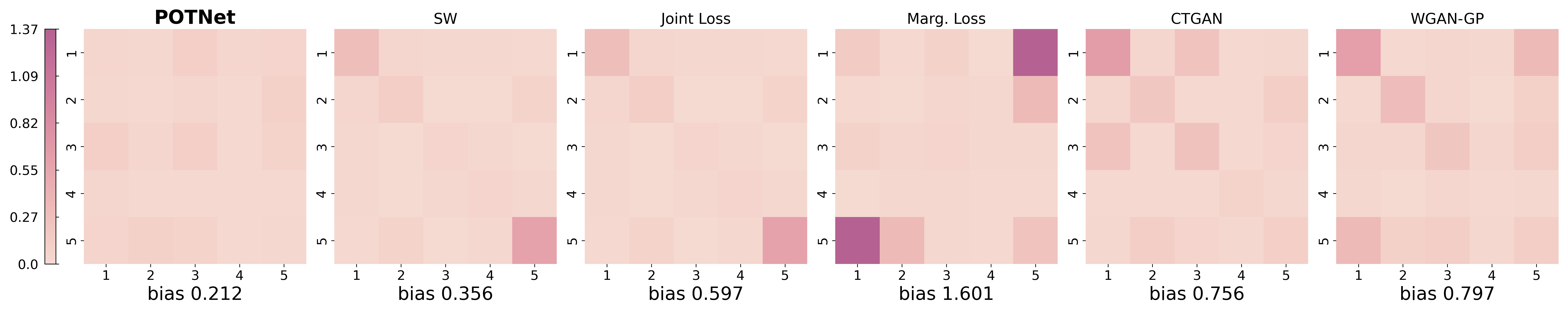
Figure 5: Difference between sample covariance matrices with respect to the ground truth; lighter color indicates smaller difference. Spectral norm of this difference is presented beneath the figures.

We also present the pairwise bivariate joint plots for the ground truth data and samples generated using POTNet, SW loss, joint loss, and marginal loss, respectively.

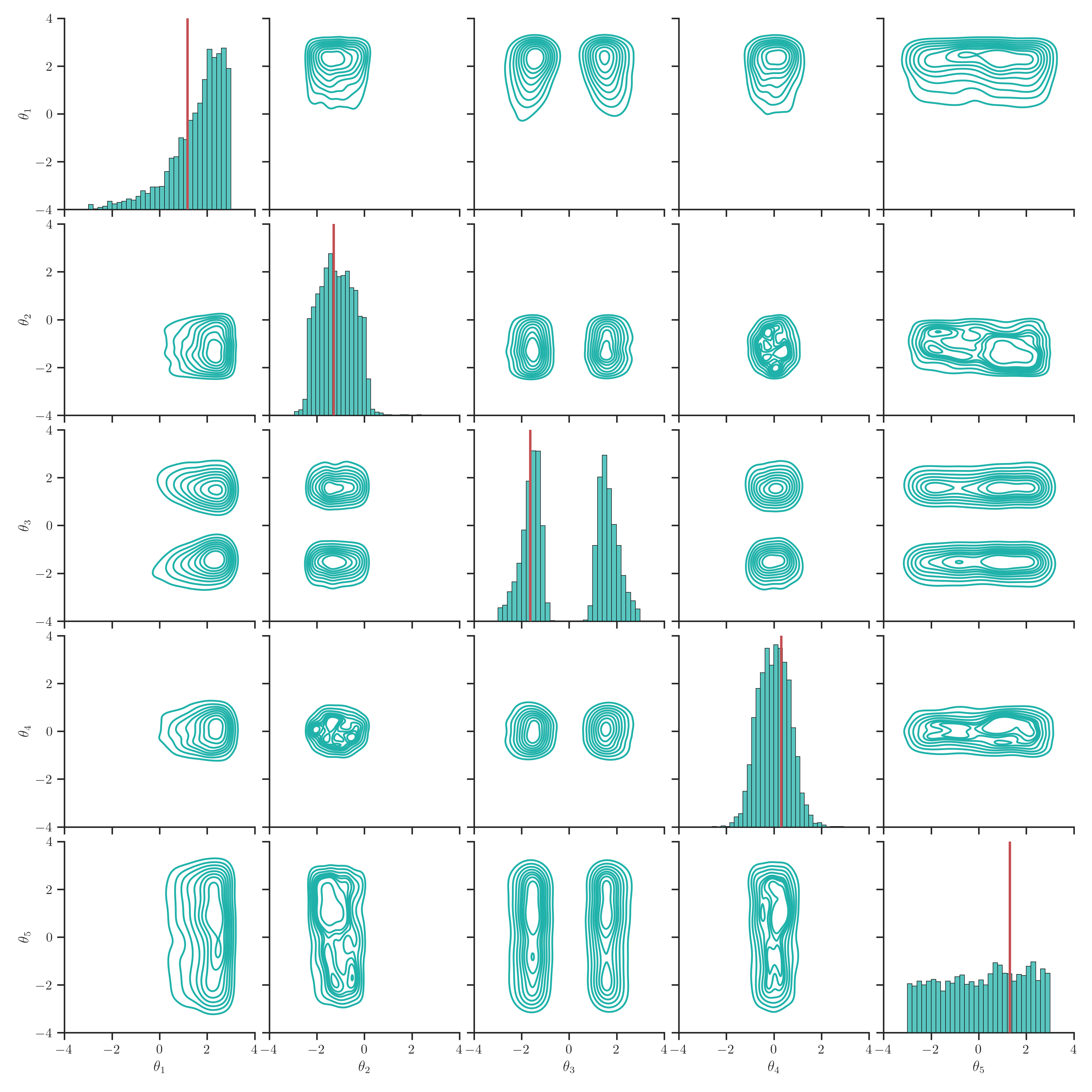
Figure 6: Samples from the true approximate posterior distribution via rejection sampling (ground truth). True parameters are indicated in red.

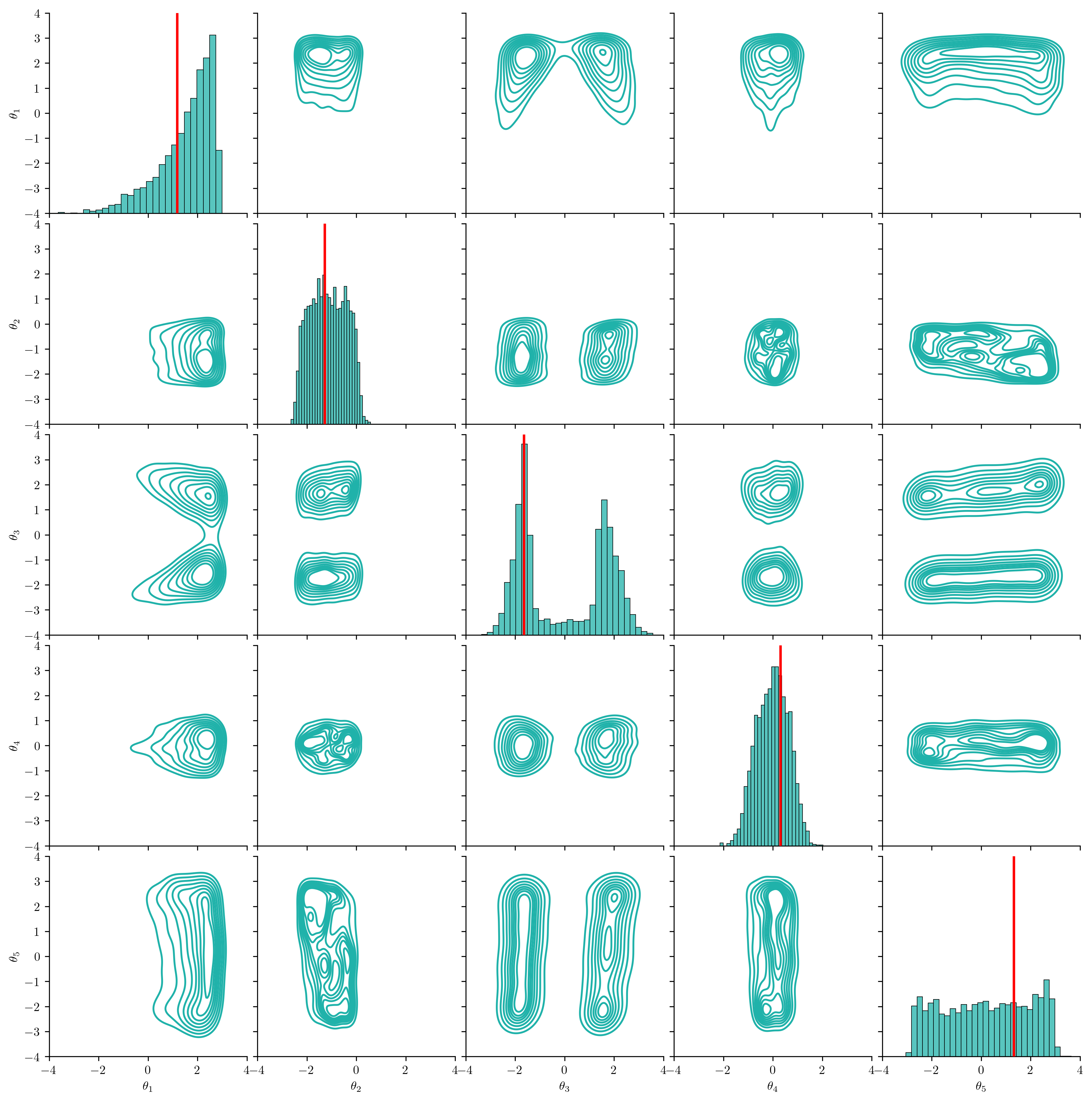
Figure 7: Samples generated by POTNet. True parameters are indicated in red.

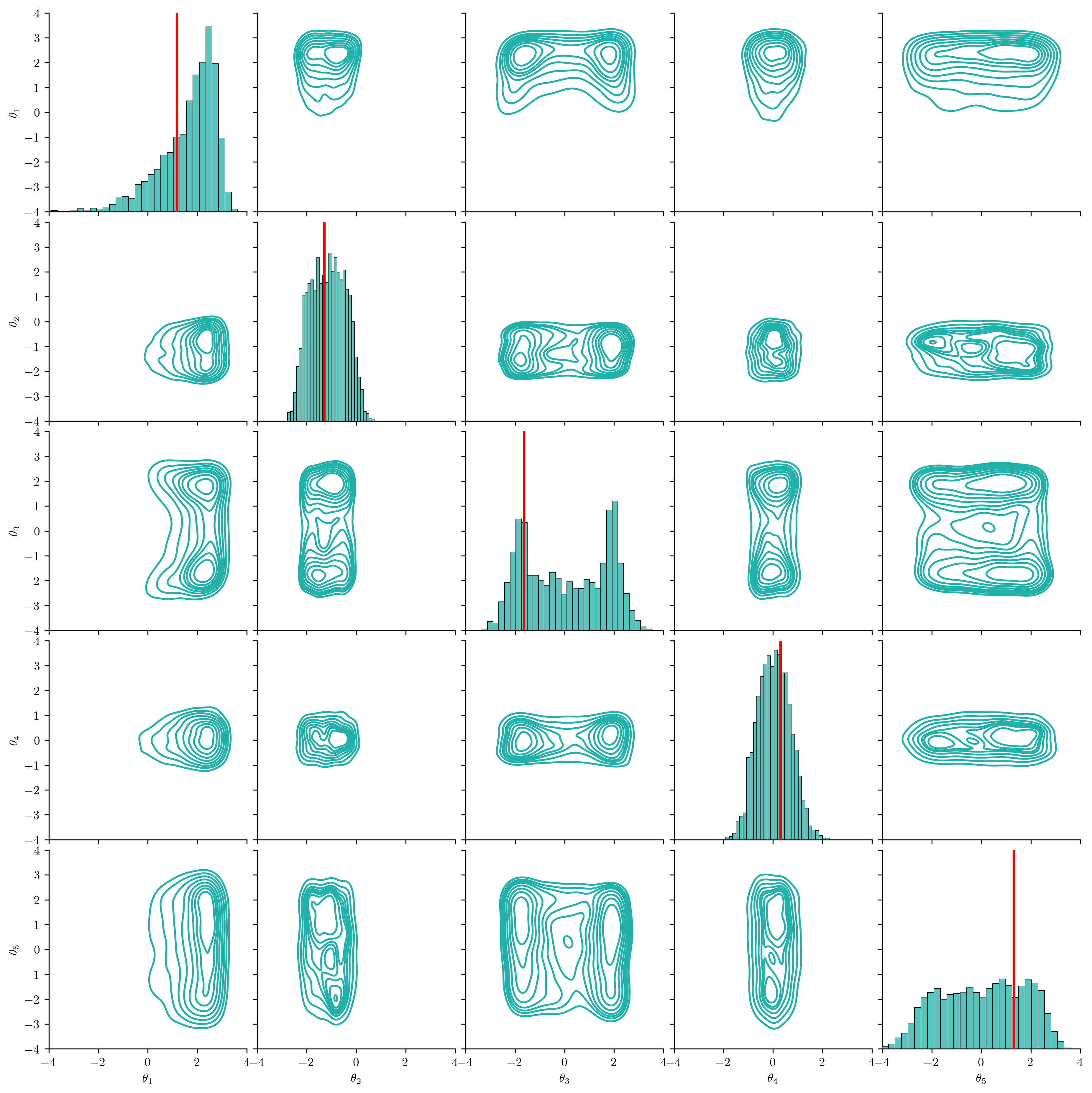
Figure 8: Samples generated using the sliced Wasserstein distance. True parameters are indicated in red.

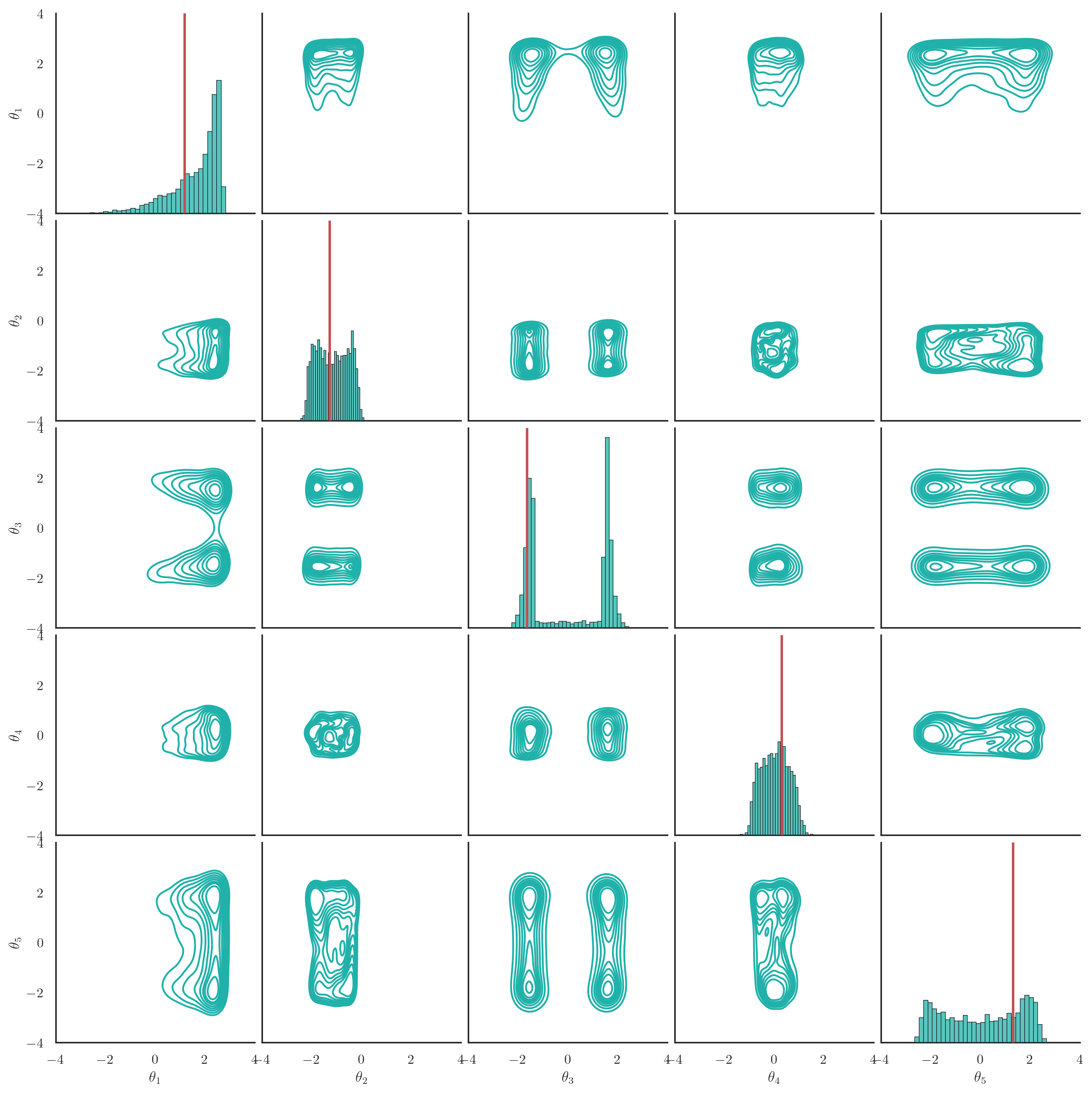
Figure 9: Samples generated by generator using only the joint loss without marginal penalties. True parameters are indicated in red.

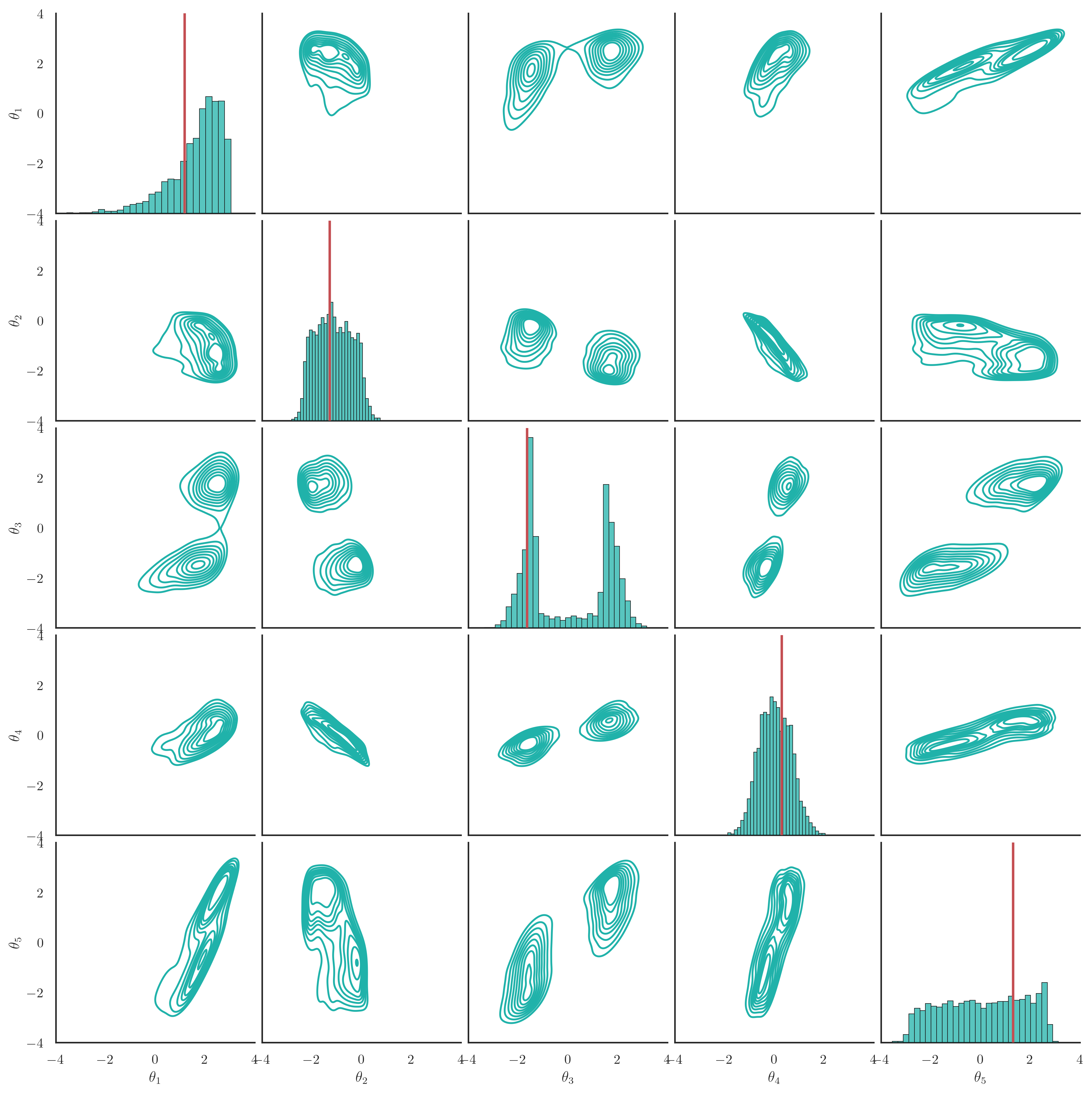
Figure 10: Samples generated by generator using only marginal losses (without the joint loss term). True parameters are indicated in red.

E.1 Pairwise density plot comparison of conditional POTNet

Figure 11: Samples from the true approximate posterior distribution via rejection sampling (ground truth). True parameters are indicated in red.

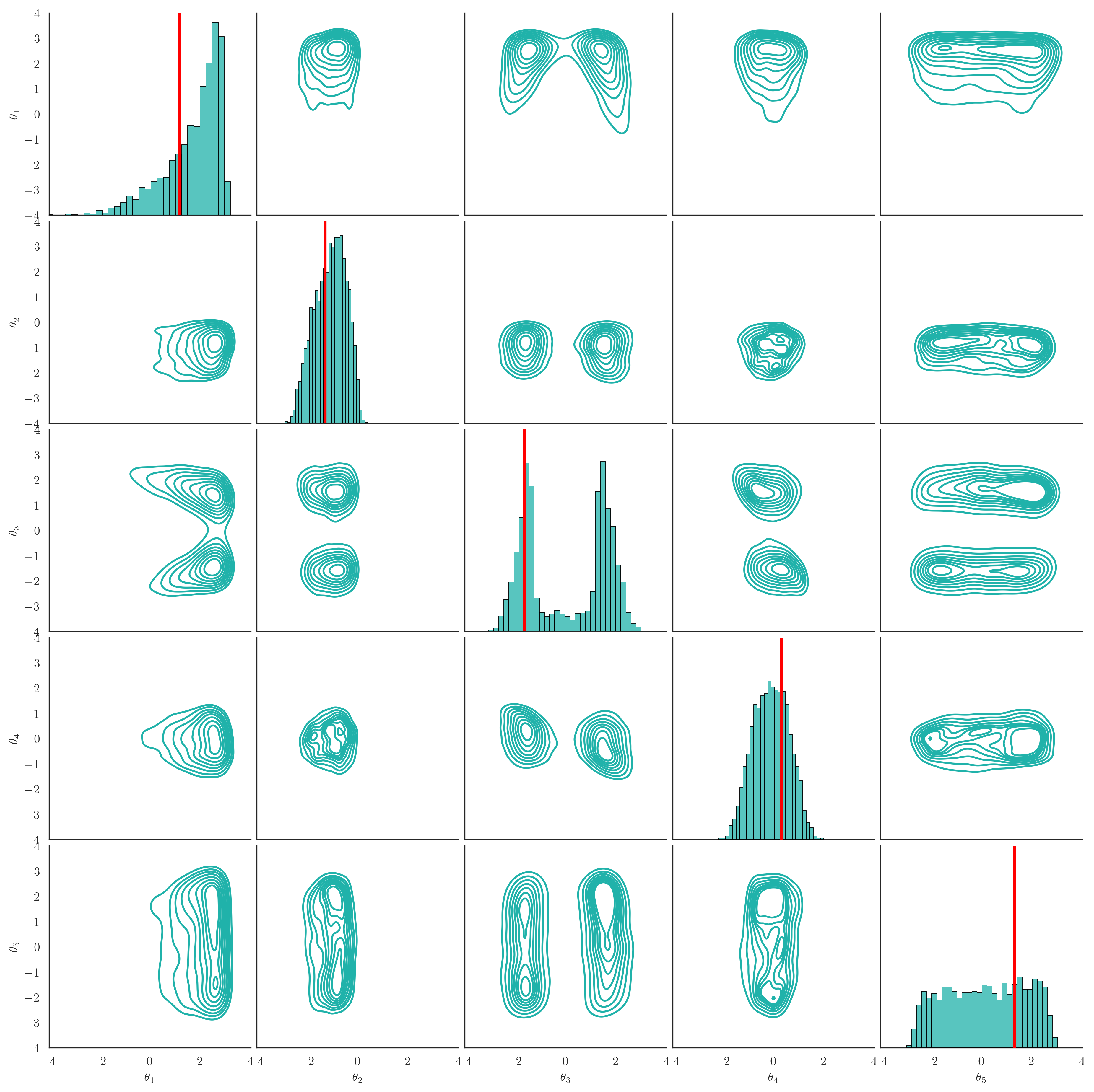
Figure 12: Samples generated by conditional POTNet and conditioning on the corresponding features $X$. True parameters are indicated in red.

Appendix F A comparison of maximum mean discrepancy (MMD) for likelihood-free inference simulated data

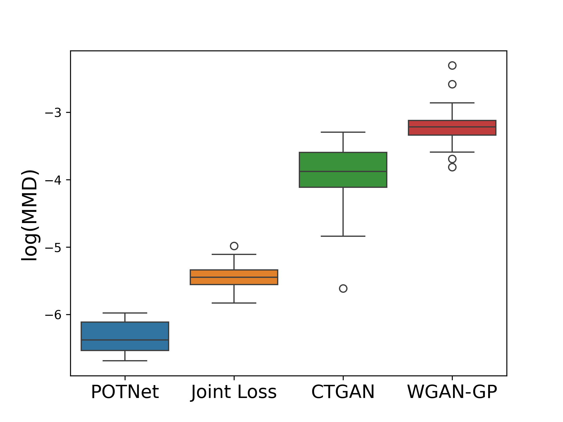
Figure 13: Maximum Mean Discrepancies (MMD, log scale) between the ground truth and the generated samples, computed over 20 iterations. Our proposed method exhibits superior performance in terms of MMD throughout 20 iterations.

Appendix G Comparison of Machine Learning Efficiency for California Housing dataset

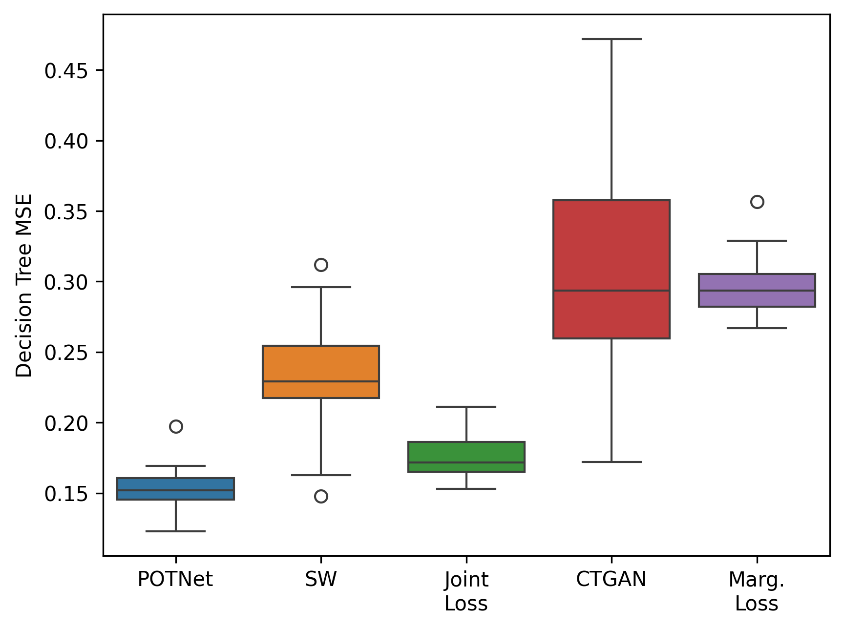
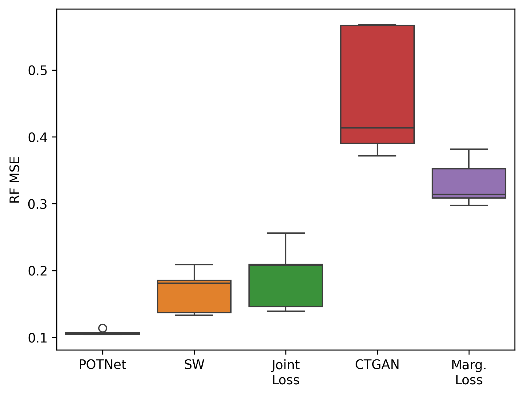
Figure 14: Machine Learning Efficiency: mean squared error evaluated on the test set using a decision tree regressor trained using synthetic data generated by each model. Lower values indicate better performance. Results obtained over 5 iterations.

Figure 15: Machine Learning Efficiency: mean squared error evaluated on the test set using a random forest regressor trained using synthetic data generated by each model. Lower values indicate better performance. Results obtained over 5 iterations.

Appendix H Comparison of Machine Learning Efficiency for Breast Cancer dataset

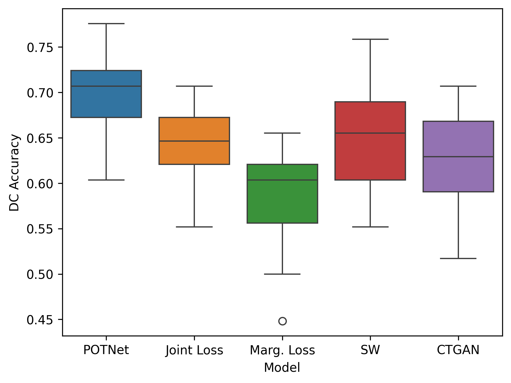
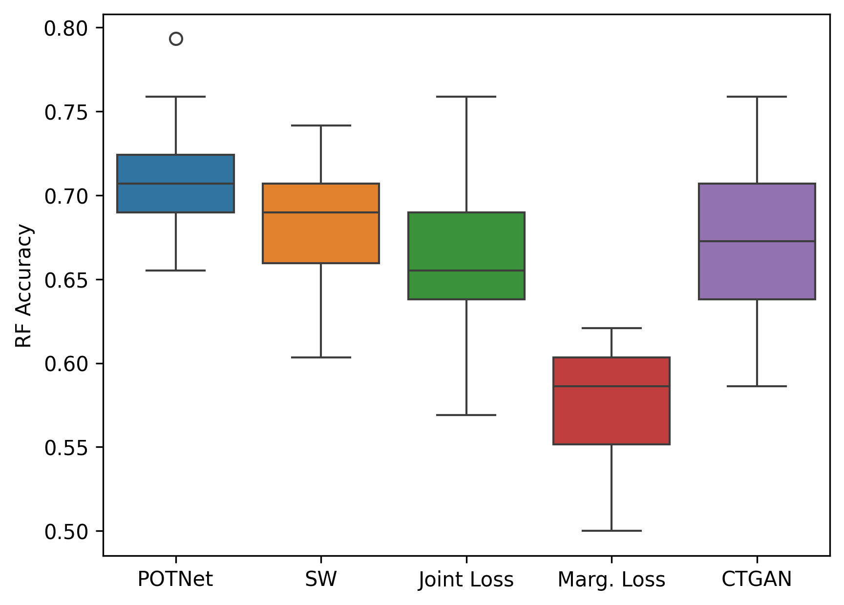
Figure 16: Machine Learning Efficiency: accuracy evaluated on the test set using a decision tree classifier trained using synthetic data generated by each model. Higher values indicate better performance. Results obtained over 5 iterations.

Figure 17: Machine Learning Efficiency: accuracy evaluated on the test set using a random forest classifier trained using synthetic data generated by each model. Higher values indicate better performance. Results obtained over 5 iterations.

Appendix I Comparison of Machine Learning Efficiency for Heart Disease dataset

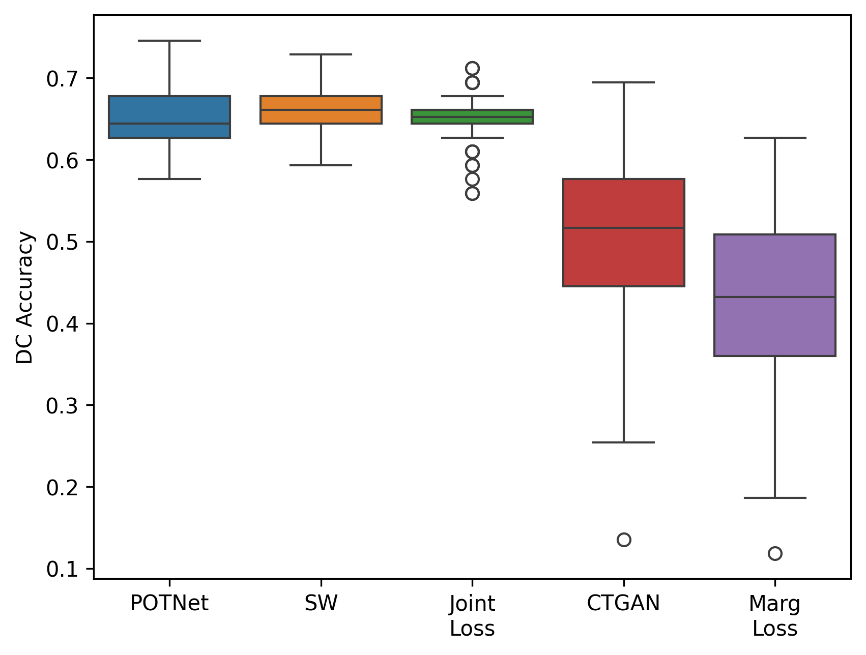
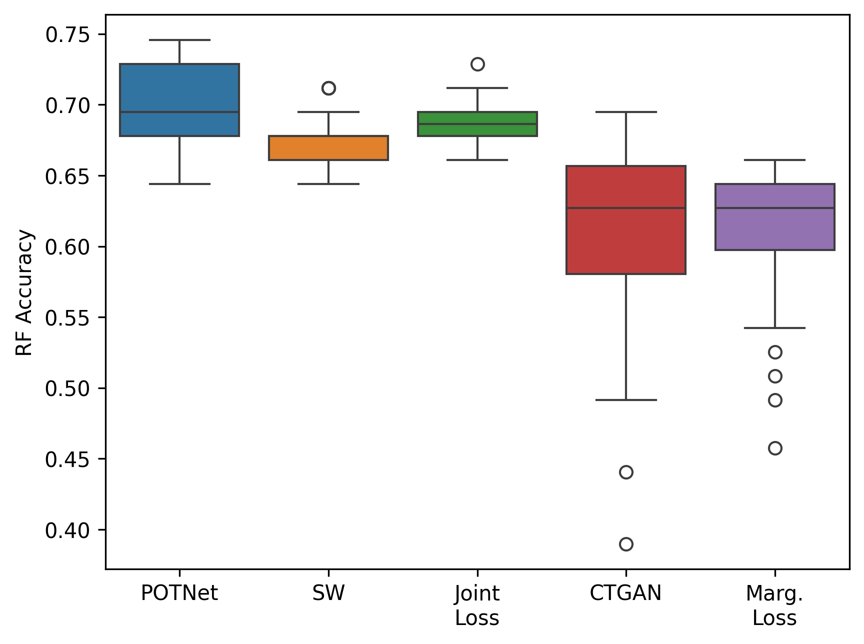
Figure 18: Machine Learning Efficiency: accuracy evaluated on the test set using a decision tree classifier trained using synthetic data generated by each model. Higher values indicate better performance. Results obtained over 5 iterations.

Figure 19: Machine Learning Efficiency: mean squared error evaluated on the test set using a random forest classifier trained using synthetic data generated by each model. Higher values indicate better performance. Results obtained over 5 iterations.

Appendix J Three-dimensional visualizations of generated samples for the likelihood-free regime

Below we present scatter plots of triviate joint distribution between synthetic samples generated by POTNet, SW model, and joint loss model. POTNet most effectively captures the joint distribution in all cases.

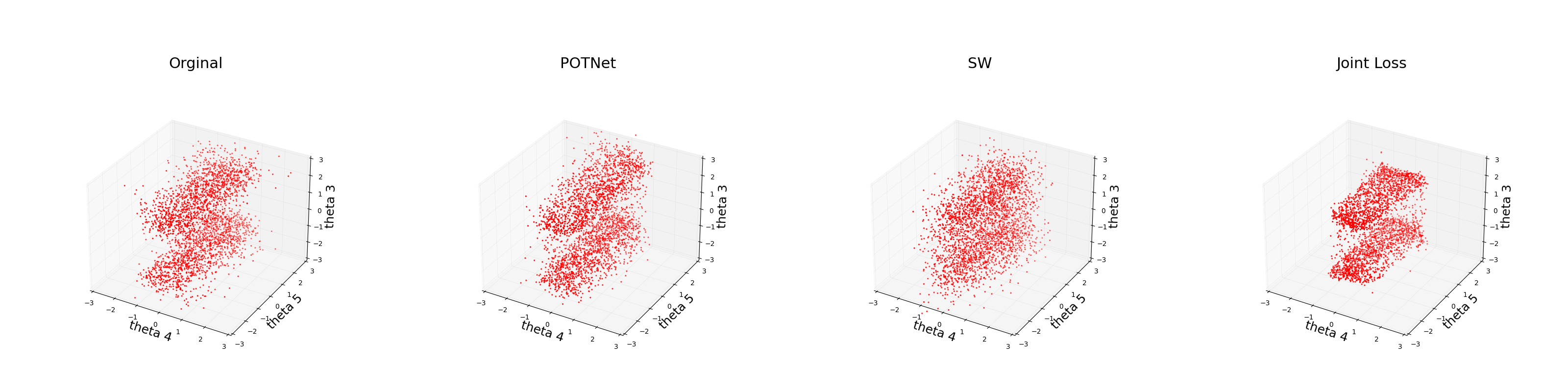
Figure 20:

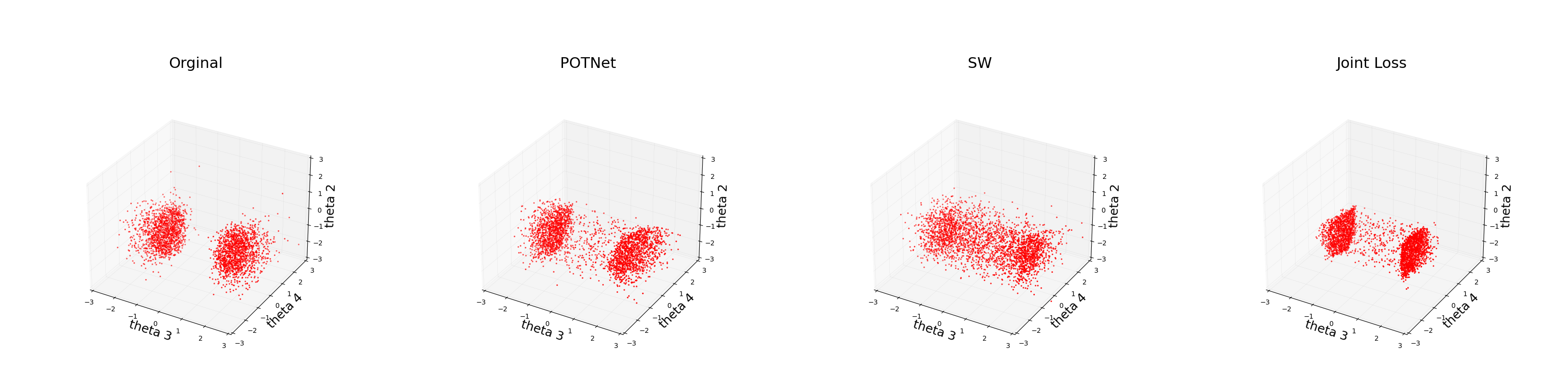
Figure 21:

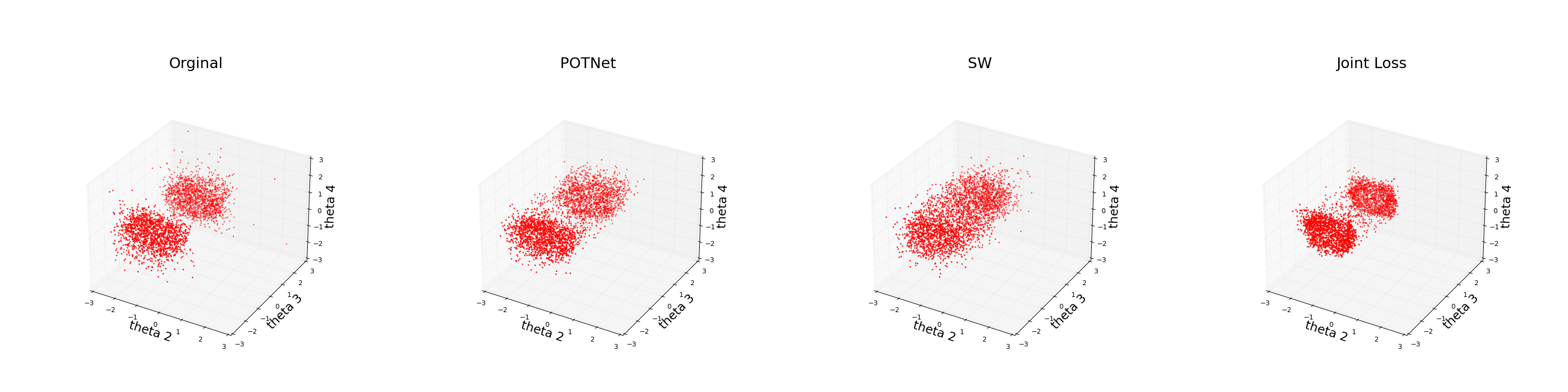
Figure 22:

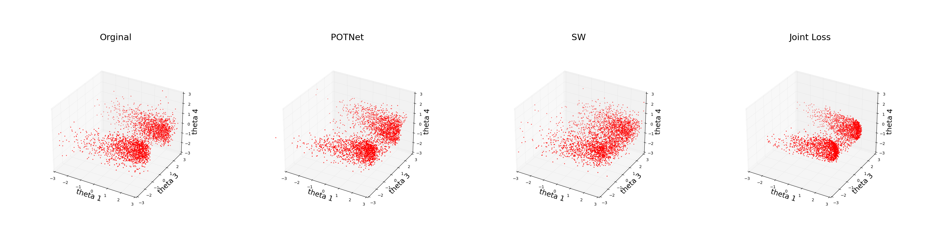
Figure 23:

References

- Arjovsky and Bottou [2017] M. Arjovsky and L. Bottou. Towards principled methods for training generative adversarial networks. arXiv preprint arXiv:1701.04862, 2017.
- Arjovsky et al. [2017] M. Arjovsky, S. Chintala, and L. Bottou. Wasserstein generative adversarial networks. In International conference on machine learning, pages 214–223. PMLR, 2017.
- Arora et al. [2017] S. Arora, R. Ge, Y. Liang, T. Ma, and Y. Zhang. Generalization and equilibrium in generative adversarial nets (gans). In International conference on machine learning, pages 224–232. PMLR, 2017.
- Beaumont [2010] M. A. Beaumont. Approximate Bayesian computation in evolution and ecology. Annual review of ecology, evolution, and systematics, 41:379–406, 2010.
- Bonneel et al. [2011] N. Bonneel, M. Van De Panne, S. Paris, and W. Heidrich. Displacement interpolation using Lagrangian mass transport. In Proceedings of the 2011 SIGGRAPH Asia conference, pages 1–12, 2011.
- Borisov et al. [2022a] V. Borisov, T. Leemann, K. Seßler, J. Haug, M. Pawelczyk, and G. Kasneci. Deep neural networks and tabular data: A survey. IEEE Transactions on Neural Networks and Learning Systems, 2022a.
- Borisov et al. [2022b] V. Borisov, K. Seßler, T. Leemann, M. Pawelczyk, and G. Kasneci. Language models are realistic tabular data generators. arXiv preprint arXiv:2210.06280, 2022b.
- Che et al. [2017] Z. Che, Y. Cheng, S. Zhai, Z. Sun, and Y. Liu. Boosting deep learning risk prediction with generative adversarial networks for electronic health records. In 2017 IEEE International Conference on Data Mining (ICDM), pages 787–792. IEEE, 2017.
- Cinquini et al. [2021] M. Cinquini, F. Giannotti, and R. Guidotti. Boosting synthetic data generation with effective nonlinear causal discovery. In 2021 IEEE Third International Conference on Cognitive Machine Intelligence (CogMI), pages 54–63. IEEE, 2021.
- Dahmen and Cook [2019] J. Dahmen and D. Cook. Synsys: A synthetic data generation system for healthcare applications. Sensors, 19(5):1181, 2019.
- Deshpande et al. [2018] I. Deshpande, Z. Zhang, and A. G. Schwing. Generative modeling using the sliced Wasserstein distance. In Proceedings of the IEEE conference on computer vision and pattern recognition, pages 3483–3491, 2018.
- Dudley [1969] R. M. Dudley. The speed of mean Glivenko-Cantelli convergence. The Annals of Mathematical Statistics, 40(1):40–50, 1969.
- Flamary et al. [2021] R. Flamary, N. Courty, A. Gramfort, M. Z. Alaya, A. Boisbunon, S. Chambon, L. Chapel, A. Corenflos, K. Fatras, N. Fournier, L. Gautheron, N. T. Gayraud, H. Janati, A. Rakotomamonjy, I. Redko, A. Rolet, A. Schutz, V. Seguy, D. J. Sutherland, R. Tavenard, A. Tong, and T. Vayer. POT: Python Optimal Transport. Journal of Machine Learning Research, 22(78):1–8, 2021. URL http://jmlr.org/papers/v22/20-451.html.
- Fonseca and Bacao [2023] J. Fonseca and F. Bacao. Tabular and latent space synthetic data generation: a literature review. Journal of Big Data, 10(1):115, 2023.
- Fournier and Guillin [2015] N. Fournier and A. Guillin. On the rate of convergence in Wasserstein distance of the empirical measure. Probability theory and related fields, 162(3-4):707–738, 2015.
- Ghassemi et al. [2020] M. Ghassemi, T. Naumann, P. Schulam, A. L. Beam, I. Y. Chen, and R. Ranganath. A review of challenges and opportunities in machine learning for health. AMIA Summits on Translational Science Proceedings, 2020:191, 2020.
- Goodfellow et al. [2014] I. Goodfellow, J. Pouget-Abadie, M. Mirza, B. Xu, D. Warde-Farley, S. Ozair, A. Courville, and Y. Bengio. Generative adversarial nets. Advances in neural information processing systems, 27, 2014.
- Gorishniy et al. [2021] Y. Gorishniy, I. Rubachev, V. Khrulkov, and A. Babenko. Revisiting deep learning models for tabular data. Advances in Neural Information Processing Systems, 34:18932–18943, 2021.
- Gretton et al. [2012] A. Gretton, K. M. Borgwardt, M. J. Rasch, B. Schölkopf, and A. Smola. A kernel two-sample test. The Journal of Machine Learning Research, 13(1):723–773, 2012.
- Gulrajani et al. [2017] I. Gulrajani, F. Ahmed, M. Arjovsky, V. Dumoulin, and A. C. Courville. Improved training of Wasserstein GANs. Advances in neural information processing systems, 30, 2017.
- Jang et al. [2016] E. Jang, S. Gu, and B. Poole. Categorical reparameterization with gumbel-softmax. arXiv preprint arXiv:1611.01144, 2016.
- Janosi et al. [1988] A. Janosi, W. Steinbrunn, M. Pfisterer, and R. Detrano. Heart Disease. UCI Machine Learning Repository, 1988. DOI: https://doi.org/10.24432/C52P4X.
- Jeffrey and Wandelt [2020] N. Jeffrey and B. D. Wandelt. Solving high-dimensional parameter inference: marginal posterior densities & Moment Networks. arXiv preprint arXiv:2011.05991, 2020.
- Jiang et al. [2017] B. Jiang, T.-y. Wu, C. Zheng, and W. H. Wong. Learning summary statistic for approximate Bayesian computation via deep neural network. Statistica Sinica, pages 1595–1618, 2017.
- Kamthe et al. [2021] S. Kamthe, S. Assefa, and M. Deisenroth. Copula flows for synthetic data generation. arXiv preprint arXiv:2101.00598, 2021.
- Kantorovich [2006] L. V. Kantorovich. On the translocation of masses. Journal of mathematical sciences, 133(4):1381–1382, 2006.
- Korotin et al. [2022] A. Korotin, A. Kolesov, and E. Burnaev. Kantorovich strikes back! Wasserstein GANs are not optimal transport? Advances in Neural Information Processing Systems, 35:13933–13946, 2022.
- Kuhn [1955] H. W. Kuhn. The Hungarian method for the assignment problem. Naval research logistics quarterly, 2(1-2):83–97, 1955.
- Loshchilov and Hutter [2017] I. Loshchilov and F. Hutter. Decoupled weight decay regularization. arXiv preprint arXiv:1711.05101, 2017.
- Lu et al. [2013] L. Lu, H. Jiang, and W. H. Wong. Multivariate density estimation by Bayesian sequential partitioning. Journal of the American Statistical Association, 108(504):1402–1410, 2013.
- Nekvi et al. [2023] R. I. Nekvi, S. Saha, Y. Al Mtawa, and A. Haque. Examining generative adversarial network for smart home ddos traffic generation. In 2023 International Symposium on Networks, Computers and Communications (ISNCC), pages 1–6. IEEE, 2023.
- Nott et al. [2014] D. J. Nott, Y. Fan, L. Marshall, and S. Sisson. Approximate Bayesian computation and Bayes’ linear analysis: toward high-dimensional ABC. Journal of Computational and Graphical Statistics, 23(1):65–86, 2014.
- Pace and Barry [1997] R. K. Pace and R. Barry. Sparse spatial autoregressions. Statistics & Probability Letters, 33(3):291–297, 1997.
- Papamakarios et al. [2019] G. Papamakarios, D. Sterratt, and I. Murray. Sequential neural likelihood: Fast likelihood-free inference with autoregressive flows. In The 22nd International Conference on Artificial Intelligence and Statistics, pages 837–848. PMLR, 2019.
- Rabin et al. [2012] J. Rabin, G. Peyré, J. Delon, and M. Bernot. Wasserstein barycenter and its application to texture mixing. In Scale Space and Variational Methods in Computer Vision: Third International Conference, SSVM 2011, Ein-Gedi, Israel, May 29–June 2, 2011, Revised Selected Papers 3, pages 435–446. Springer, 2012.
- Salimans et al. [2016] T. Salimans, I. Goodfellow, W. Zaremba, V. Cheung, A. Radford, and X. Chen. Improved techniques for training gans. Advances in neural information processing systems, 29, 2016.
- Salmona et al. [2022] A. Salmona, V. De Bortoli, J. Delon, and A. Desolneux. Can push-forward generative models fit multimodal distributions? Advances in Neural Information Processing Systems, 35:10766–10779, 2022.
- Shwartz-Ziv and Armon [2022] R. Shwartz-Ziv and A. Armon. Tabular data: Deep learning is not all you need. Information Fusion, 81:84–90, 2022.
- Villani et al. [2009] C. Villani et al. Optimal transport: old and new, volume 338. Springer, 2009.
- Wang and Ročková [2022] Y. Wang and V. Ročková. Adversarial Bayesian simulation. arXiv preprint arXiv:2208.12113, 2022.
- Weed and Bach [2019] J. Weed and F. Bach. Sharp asymptotic and finite-sample rates of convergence of empirical measures in Wasserstein distance. Bernoulli, 25(4A):2620–2648, 2019. ISSN 1350-7265,1573-9759. doi: 10.3150/18-BEJ1065. URL https://doi.org/10.3150/18-BEJ1065.
- Wu et al. [2019] J. Wu, Z. Huang, D. Acharya, W. Li, J. Thoma, D. P. Paudel, and L. V. Gool. Sliced Wasserstein generative models. In Proceedings of the IEEE/CVF Conference on Computer Vision and Pattern Recognition, pages 3713–3722, 2019.
- Xu et al. [2019] L. Xu, M. Skoularidou, A. Cuesta-Infante, and K. Veeramachaneni. Modeling tabular data using conditional gan. Advances in neural information processing systems, 32, 2019.
- Zhang et al. [2022] A. Zhang, L. Xing, J. Zou, and J. C. Wu. Shifting machine learning for healthcare from development to deployment and from models to data. Nature Biomedical Engineering, 6(12):1330–1345, 2022.
- Zwitter and Soklic [1988] M. Zwitter and M. Soklic. Breast Cancer. UCI Machine Learning Repository, 1988. DOI: https://doi.org/10.24432/C51P4M.