An estimator for the mean
that dominates the empirical average

Abstract

We propose a simple empirical representation of expectations such that: For a number of samples above a certain threshold, drawn from any probability distribution with finite fourth-order statistic, the proposed estimator outperforms the empirical average when tested against the actual population, with respect to the quadratic loss. For datasets smaller than this threshold, the result still holds, but for a class of distributions determined by their first four statistics. Our approach leverages the duality between distributionally robust and risk-averse optimization.

1 Introduction

Although expectations achieve the least value of the mean squared error, they often have to be estimated empirically by averaging on a set of samples drawn from an unknown probability distribution. While averaging behaves like the population mean in the long run, we often infer about the actual population based on limited data. In such cases, averaging exhibits sub-optimal mse performance when tested against the actual population, and thus, despite its simplicity, it is rather an arbitrary choice . That said, in this study we state the following motivating question:

Is there an algorithm that outperforms the
empirical average w.r.t. the mean square error?

Since it is the lack of mass that prevents the empirical average from performing well, one idea is to search for an appropriate re-weighting of the available data that, when followed by averaging, matches, or at least approaches the actual expected value in some well-defined distance. One approach for finding such a distributional shift is given by distributionally robust optimization (DRO). On top of that, a simple implementation of expectations asks for a distributionally robust mean squared error problem that is solvable in closed form. Thus, our initial question reduces to whether such a problem exists. In some cases, robustness against distributional shifts is as safeguarding against risky events (naturally coordinated by the distribution’s tail). Such a dual relation suggests a place to start our design.

To set up the stage for our investigation, on a probability space $(\Omega,\mathrm{F},\mu)$, consider a random vector ${\Theta}:\Omega\rightarrow\mathbb{R}^{d}$ distributed according to the unknown probability distribution $\mu_{\Theta}$. We are interested in estimating $\mathbb{E}{\Theta}$ based on i.i.d. data by means of an estimator $\widehat{{\Theta}}\in\mathbb{R}^{d}$. With the data generating distribution $\mu_{\Theta}$ being unknown, averaging corresponds to the solution of the empirical risk minimization problem $\min_{\widehat{\Theta}}Q(\widehat{\Theta})\equiv n^{-1}\sum^{n}_{i=1}\|\widehat{\Theta}-\Theta_{i}\|^{2}_{2}$, which is a surrogate of the mmse problem

$$\min_{\widehat{\Theta}\in\mathbb{R}^{d}}\mathbb{E}\|\widehat{\Theta}-\Theta\|^{2}_{2}.$$ (1)

Therefore, if we wish to devise an algorithm other than averaging for estimating $\mathbb{E}\Theta$, we need to start by first placing a problem with the aforesaid desired features (i.e., distributional robustness and closed form representation). To this end, we consider the following risk-constrained extension of (1)

$$\begin{array}[]{cl}\underset{\widehat{{\Theta}}\in\mathbb{R}^{d}}{\operatorname{min}}&\mathbb{E}~{}\|{\Theta}-\widehat{{\Theta}}\|_{2}^{2}\\ \text{ s.t. }&\mathbb{E}\big{(}\|{\Theta}-\widehat{{\Theta}}\|_{2}^{2}~{}-~{}\mathbb{E}\|{\Theta}-\widehat{{\Theta}}\|_{2}^{2}\big{)}^{2}\leq\varepsilon,\end{array}$$ (2)

where all expectations are taken w.r.t. $\mu$. Problem (2) is a quadratically constrained quadratic program (see Section 2) that in principle can be solved in closed form. Therefore, it is a candidate risk-constrained mmse problem and whether or not its solution answers positively our question remains to be verified. On our way there, our contributions are as follows:

1.1 Contributions

• The risk-constrained estimator as a stereographic projection.
  We observe that the constraint of (2) can be written as a perfect square, thus allowing us to view the solution of (2) as the stereographic projection of the mmse sphere onto the subspace $\mathbb{R}^{d}$. Subsequently, taking advantage of the Lagrangean duality, we solve (2) by completing the squares.

• Relation with Fisher’s moment coefficient of skewness.
  We find that the bias between the stereographic and the traditionally deployed orthogonal projection is composed by fractions of the Fisher’s skewness coefficient, and additional terms that capture the cross third-order statistics of the state, the latter as seen through the available information.

• Risk constrained estimator as a weighted average.
  Being guided by the geometric picture and the Lagrangean of the problem, we express the solution of (2) as a weighted sum through a fixed point equation. The latter linear combination becomes a weighted average within a computable range of the Lagrange multiplier associated with the constraint of (2).

• Fisher’s coefficient of skewness and the $2-$Wasserstein gradient of $\chi^{2}-$divergence.
  We demonstrate that Fisher’s moment coefficient of skewness can be expressed as a fraction of the expected $2-$Wasserstein gradient of the $\chi^{2}-$divergence, thus interpreting the directionality of the re-weighting.

• Distributionally robust mean squared error estimator $\mathrm{(DRMSEE)}$.
  Taking into account the relation between the Lagrangean of (2) and the mean-deviation risk measure of order $p=2$ (i.e., the mean-standard deviation risk measure), we show that the aforesaid weighted average solves the $\chi^{2}-$ distributionally robust mse estimation problem for all $\chi^{2}-$ radii inside the previously mentioned range.

• Generalization.
  We show that after a certain number of samples $n_{g}$ drawn from any probability distribution with finite fourth order moment, there exist a value $\lambda_{g}$ of $\lambda$ below which the empirical DRMSEE generalizes strictly better than the empirical average w.r.t. the quadratic loss. In addition, when the samples are less than $n_{g}$, the result still holds, but for a class of probability distributions determined by their first four statistics.

1.2 Roadmap

Expectations are the solution to the minimum mean squared error (mmse) estimation problem (Girshick and Savage, 1951; James and Stein, 1961; Devroye et al., 2003; Wang and Bovik, 2009; Verhaegen and Verdult, 2007; Kuhn et al., 2019) and are usually estimated by averaging over a set of samples. In many cases in statistics and machine learning though, such a set is limited and the lack of mass induces naturally an uncertain distributional shift from the actual measure (Duchi and Namkoong, 2018; Gotoh et al., 2018).

Distributionally robust optimization serves as a formulation paradigm in applications where the underlying distribution is partially known or completely unknown. This distributional uncertainty w.r.t. the population at hand, is expressed by an uncertainty set of probability distributions. The two main approaches for representing the uncertainty set, recently unified by (Blanchet et al., 2023), are the divergence approach, and the Wasserstein approach. In the former one, distributional shifts are measured in terms of likelihood ratios (Bertsimas and Sim, 2004; Bayraksan and Love, 2015; Namkoong and Duchi, 2016; Duchi and Namkoong, 2018; Van Parys et al., 2021; Blanchet et al., 2023), while in the latter, the ambiguity set is represented by a Wasserstein ball (Esfahani and Kuhn, 2015; Gao and Kleywegt, 2023; Lee and Raginsky, 2018; Kuhn et al., 2019; Blanchet et al., 2023).

On the other hand, risk-averse optimization refers to the optimization of risk measures. Unlike expectations, these are convex functions defined on the space of random variables and deliver optimizers that take into account the risky events of the underlying distribution (coordinated by the distribution’s tail). Being convex, a risk measure can be seen through the Legendre transform as the supremum of its affine minorants that is, as a family of expectations, over a subset of the (dual) space of (in general signed) measures (Shapiro et al., 2021).

For the particular class of coherent risk measures, this set contains probability measures and thus, safeguarding for risky events is as being robust against distributional shifts. In other words, solving a risk-constrained problem on the population at hand is as solving a min-max problem where expectations are taken for an appropriate re-weighting of that population.

That being said, minimization of risk, does not always correspond to a (DRO) problem, and vice versa. In our study, problem (2) is closely related to the mean-variance risk measure (Shapiro et al., 2021, p. 275), which does not lead to a distributionally robust problem in general. However, the mean deviation risk measure of order $p=2$ does, and it is also closely related to (2) (see Section 3). Our goal then is to examine if such a re-weighting of the underlying data indeed places the average closer to the expectation under a well-defined distance. If it does, the corresponding (re-weighted) empirical average serves as a more suitable algorithm for the mean w.r.t. the mse.

1.3 Related work

Mean square error estimation has received interest over the years (Girshick and Savage, 1951; Stein, 1956; James and Stein, 1961; Devroye et al., 2003; Wang and Bovik, 2009; Nguyen et al., 2023) not only because mean squared error (mse) serves as the long standard for measuring the adequacy of an estimator, but also because many problems in statistics can be recast to mean squared error estimation problems (Verhaegen and Verdult, 2007). Under the theory of Hilbert spaces, expectations can be defined as the orthogonal projections w.r.t. the induced norm and as such, they are the minimizers of the mse problem.

Mean-variance optimization was initially utilized by (Markowitz, 1952), in portfolio selection. Later on, (Abeille et al., 2016) deploys mean-variance for dynamic portfolio allocation problems, and (Kalogerias et al., 2020) stressed the importance of safeguarding against risky events in mean squared error Bayesian estimation. Further, (Wu et al., 2018; Shapiro et al., 2023) introduced the Bayesian Risk Optimization (BRO) formulation in which the risk functional is applied to the posterior distribution, and studied the mean-variance risk measure as a special case.

Distributionally robust optimization was introduced by (Scarf et al., 1957) and aims to produce solutions that perform well for a class of problems, all parameterized by a distribution in an uncertainty set. As a paradigm it has gain interest due to its connections to regularization, generalization, and robustness (Staib and Jegelka, 2019). In machine learning, the two main approaches for representing the uncertainty set of the DRO problem, have led to a number of structural results. For example, DRO with $\chi^{2}$-divergence is almost equivalent as controlling by the variance (Gotoh et al., 2018; Lam, 2016; Duchi and Namkoong, 2019) were the worst case measure is computed exactly in $O(n\log(n))$ (Staib and Jegelka, 2019). Further, (Staib and Jegelka, 2019) shows that maximum mean discrepancy DRO is almost equivalent to regularization by the Hilbert norm. In addition, (Gotoh et al., 2021) develops a theory for selecting the risk-aversion parameter (or level of robustness) of the distributionally robust formulation. Lastly, (Nguyen et al., 2023) introduced a distributionally robust minimium mean square error estimation model with a Wasserstein ambiguity set, and provided a solution by developing a numerical algorithm. Further,  (Blanchet et al., 2021) gives a statistical analysis of Wasserstein distributionally robust estimators.

Stein’s paradox (Efron and Morris, 1977) has a significant impact on high-dimensional statistics, suggesting that relying exclusively on the sample mean as the default estimator may not be the most effective approach in higher dimensions. To tackle this issue, the James-Stein estimator suggests improving estimation accuracy by adjusting the sample means towards a more centralized mean vector. The James-Stein estimator is a significant concept in statistical theory, particularly concerning the calculation of the mean in a multivariate normal distribution. Traditionally, statisticians rely on the sample mean, also known as the maximumlikelihood estimator. However, in situations where the means of multiple correlated Gaussian distributed random vectors are unknown, the James-Stein estimator, despite its bias, is preferred. This estimator was initially introduced by Charles Stein in 1956 (Stein, 1956) , revealing a surprising result: while the standard mean estimate is acceptable when dealing with two or fewer correlated vectors, it becomes unacceptable for three or more. This revelation led to the proposal of an improved estimator that involves adjusting the sample means towards a central vector of means, a concept often referred to as Stein’s paradox. The James-Stein estimator often achieves a lower mse compared to using the sample mean alone, especially when the sample size is small relative to the number of parameters being estimated. The James-Stein estimator has inspired extensive research exploring the concept of ‘shrinkage’ within statistics. Some notable examples include LASSO (Tibshirani, 1996), ridge regression (Hoerl and Kennard, 1970), the Ledoit-Wolf covariance estimator (Ledoit and Wolf, 2004), and Elastic Net (Zou and Hastie, 2005).

2 Risk-constrained minimum mean squared error estimators

We begin analyzing the risk-constrained mmse problem (2) by first referring the reader to (Kalogerias et al., 2019, Lemma 1), where the well-definiteness of the statement (2) is ensured under the following regularity condition

Assumption 1

It is true that $\int\|{\theta}\|_{2}^{3}~{}\mathrm{d}\mu_{{\Theta}}(\theta)<+\infty\text{.}$

By noticing that the constraint in (2) can be written as a perfect square, we establish a quadratic reformulation that on the one hand, allows us to interpret the solution to (2) as a stereographic projection, and on the other, sets the stage for a derivative-free solution:

Lemma 1 (The risk-constrained estimator as stereographic projection)

Under
Assumption 1, problem (2) is well-defined and equivalent to the convex quadratic program

$$\begin{array}[]{cl}\underset{\widehat{{\Theta}}\in\mathcal{L}_{2}}{\mathrm{min}}&\mathbb{E}\|{\Theta}-\widehat{\Theta}\|^{2}_{2}\\ \mathrm{s.t.}&\|\widehat{\Theta}-\frac{1}{4}\Sigma^{-1}_{\Theta}\zeta^{-}\|^{2}_{4\Sigma_{\Theta}}\leq\bar{\varepsilon}\end{array}$$ (3)

where $\zeta^{-}=2\big{(}\mathbb{E}\big{[}\|{\Theta}\|^{2}_{2}{\Theta}]-\mathbb{E}\|{\Theta}\|^{2}_{2}\mathbb{E}\Theta\big{)}$, $\bar{\varepsilon}=\varepsilon+(\zeta^{-})^{\top}\frac{\Sigma^{-1}_{{\Theta}|{X}}}{4}\zeta^{-}-\alpha$, $\alpha=\mathbb{E}(||\Theta||^{2}-\mathbb{E}||\Theta||^{2})^{2}$ and ${\Sigma}_{{\Theta}}\succcurlyeq{0}$ is the covariance matrix of $\Theta$ .

Lemma 1 shows the equivalence of (2) to the convex quadratic program (3) allowing to interpret the former in geometric terms based on the standard inner product in $\mathbb{R}^{d}$. Within this setting, the solution to (46) is a stereographic projection of the $\mathrm{mmse}-$sphere onto the subspace of the square integrable estimators. Further, we can do slightly more by applying Pythagora’s theorem to the objective in (3) to obtain

$$\begin{array}[]{cl}\underset{\widehat{{\Theta}}\in{\mathbb{R}^{d}}}{\mathrm{min}}&\|\widehat{{\Theta}}-\mathbb{E}\Theta\|^{2}_{2}\\ \mathrm{s.t.}&\|\widehat{{\Theta}}-\frac{1}{4}{\Sigma}^{-1}_{\Theta}\zeta^{-}\|^{2}_{4{\Sigma_{\Theta}}}\leq{\bar{\varepsilon}},\end{array},$$ (4)

where by $\zeta^{-}$ we mean the opposite vector to $\zeta$. According to Lemma 1, the solution of (4) (and therefore of (2)) is the point lying on the ellipse of ‘radius’ $\bar{\varepsilon}>0$ and of center $\frac{1}{4}{\Sigma}^{-1}_{\Theta}\zeta$, that has the least quadrance from the orthogonal projection $\mathbb{E}\Theta$.

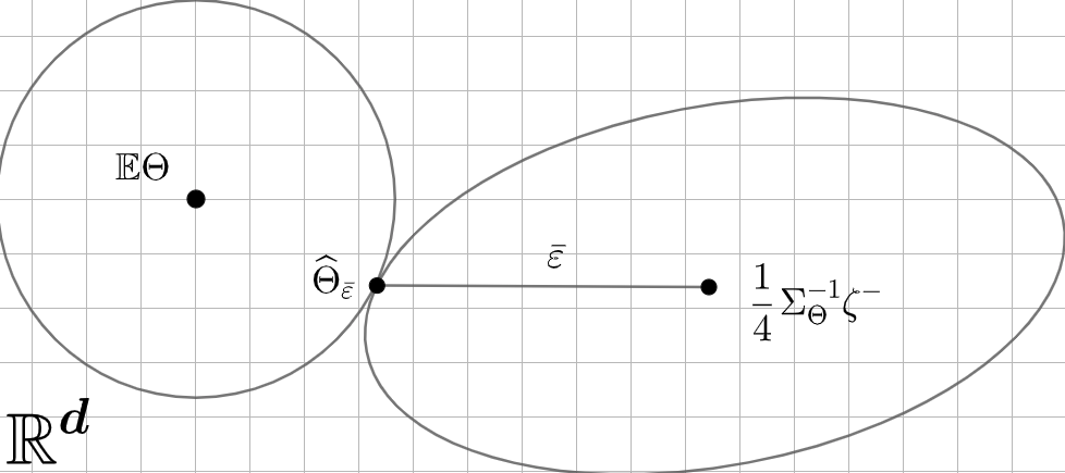
Figure 1: The solution to the ${\varepsilon}-$risk-averse mmse problem is the point on the ellipse of ‘radius’ $\bar{\varepsilon}\geq 0$ and center $\frac{1}{4}\Sigma^{-1}_{\Theta}\zeta^{-}$ that has the least distance from $\mathbb{E}\Theta$.

Guided by the geometric picture (see e.g. Figure 1), we observe that the problem is feasible for any $\bar{\varepsilon}\geq{0}$. In particular, for all $\bar{\varepsilon}\geq\bar{\varepsilon}_{cr}$,  $\bar{\varepsilon}_{cr}=\|{\mathbb{E}\Theta-\frac{1}{4}{\Sigma}^{-1}_{\Theta}\zeta^{-}\|^{2}_{4{\Sigma}_{\Theta}}}$, $\widehat{\Theta}^{*}=\mathbb{E}\Theta$, while for $\bar{\varepsilon}=0$, a solution exists only when $\mathbb{E}\Theta=\frac{1}{4}\Sigma^{-1}_{\Theta}\zeta^{-}$. Moving forward, for all $\bar{\varepsilon}\in(0,\bar{\varepsilon}_{c})$ the solution is the unique touching point of the circle and the ellipse and it is obtained by equating the “equilibrium forces”. However, due to the favorable structure provided by Lemma 1, we may proceed derivative-free (see Appendix A).

Proposition 1 (The risk-constrained mmse estimator)

Under the Assumption 1, the optimal solution to (2) is

$$\widehat{\Theta}^{*}_{\lambda^{*}}{=}\big{(}I+4\lambda^{*}\Sigma_{\Theta}\big{)}^{-1}\Big{(}\mathbb{E}\Theta+2\lambda^{*}\big{(}\mathbb{E}[\|\Theta\|^{2}_{2}\Theta]-\mathbb{E}\|\Theta\|^{2}_{2}\mathbb{E}\Theta\big{)}\Big{)},$$ (5)

where $\lambda^{*}\geq{0}$ is the solution to the corresponding dual problem.

Because by construction, (2) aims to reduce the estimation error variability, it is expected to do so by shifting the optimal estimates towards the areas suffering high loss, that is, towards the tail of the underlying distribution. The next result characterizes the bias of (5): The DRMSEE is a shifted version of the conditional expectation by a fraction of the conditional Fisher’s moment coefficient of skewness plus the cross third-order statistics of the state.

Corollary 1 (Risk-constrained mmse estimator and Fisher’s skewness)

The estimator (5) operates according to

$$\widehat{{\Theta}}^{*}_{i,u,\lambda} =\mathbb{E}{\Theta}_{i,u}{+}\frac{\lambda\sigma_{i}\sqrt{\sigma_{i}}}{1+2\lambda\sigma_{i}}\mathbb{E}\left(\frac{{\Theta}_{i,u}-\mathbb{E}{\Theta}_{i,u}}{\sqrt{\sigma_{i}}}\right)^{3}{+}\mathrm{T}_{i,\lambda},$$ (6)

where ${\Theta}_{i,u}$, and $\widehat{{\Theta}}^{*}_{i,u,\lambda}$ denotes the $i$th component of ${\Theta}_{u}\equiv U^{\top}{\Theta}$, and $U^{\top}\widehat{{\Theta}}^{*}_{\lambda}$, respectively, $U$ the orthonormal matrix with columns the eigen-vectors of ${\Sigma}_{{\Theta}}$, and

$$\small\mathrm{T}_{i,\lambda}=\frac{\lambda}{1+2\lambda\sigma_{i}}\sum_{k\neq{i}}\mathbb{E}{\Theta}^{2}_{k,u}\mathbb{E}{\Theta}_{i,u}-\mathbb{E}[{\Theta}^{2}_{k,u}{\Theta}_{i,u}].$$

In an effort to minimize the squared error on average while maintaining its variance small, DRMSEE attributes the estimation error made by the conditional expectation to the skewness of the conditional distribution along the eigendirections of the conditional expected error. In particular, in the one-dimensional case, cross third-order statistics are non-existent and therefore,

$$\widehat{{\Theta}}^{*}_{\lambda}=\mathbb{E}\Theta+\frac{\lambda\sigma\sqrt{\sigma}}{1+2\lambda\sigma}\mathbb{E}\Bigg{(}\frac{\Theta-\mathbb{E}{\Theta}}{\sqrt{\sigma}}\Bigg{)}^{3}~{},~{}\lambda\in[0,+\infty).$$ (7)

Corollary 1 reveals the “internal mechanism” with which (5) biases towards the tail of the underline distribution. Per error eigen-direction, the DRMSEE compensates for the high losses relative to the conditional expectation, by a fraction of the Fisher’s skewness coefficient and a term $\mathrm{T}_{i}$, that captures the cross third-order statistics of the state components. Although (6) involves the cross third-order statistics of the projected state, these statistics cannot emerge artificially from a coordinate change such as $U^{\top}{\Theta}$, but are intrinsic to the conditional state itself. Besides, a meaningfull measure of risk should always be coordinate change invariant.

Motivated by the Figure 1, and the Lagrangean of (2), we note that there exists a unique random element such that (5) is viewed as its corresponding average. Fortunately, such an element can be expressed as a Radon-Nikodym derivative w.r.t. $\mu_{\Theta}$.

Lemma 2 (Risk constrained estimator as a weighted average)

The optimal solution of (2) can be written as

$$\widehat{\Theta}^{*}_{\lambda}=\mathbb{E}_{\xi_{\Theta}(\widehat{\Theta}^{*}_{\lambda},\lambda)}\Theta,$$ (8)

where

$$\frac{\mathrm{d}{\mu_{\Theta}}}{\mathrm{d}\xi_{\Theta}}\equiv 1+2\lambda\big{(}\|\Theta-\widehat{\Theta}^{*}_{\lambda}\|^{2}_{2}-\mathbb{E}\|\Theta-\widehat{\Theta}^{*}_{\lambda}\|^{2}_{2}\big{)}.$$ (9)

In particular, for $\lambda\leq{1}/{\gamma^{*}}$, $\gamma^{*}=2\big{(}\mathbb{E}\|\widehat{\Theta}^{*}_{\infty}-\widehat{\Theta}^{*}_{0}\|^{2}_{2}+\mathrm{mmse}(\mu_{\Theta})\big{)}$, it follows that $\frac{\mathrm{d}{\mu_{\Theta}}}{\mathrm{d}\xi_{\Theta}}\geq{0}$.

Combining Lemma 2 and (7), we obtain

$$\mathbb{E}_{\xi_{\lambda}}\Theta=\mathbb{E}_{\mu}\Theta+\frac{\lambda\sigma\sqrt{\sigma}}{1+2\lambda\sigma}\mathbb{E}_{\mu}\left(\frac{\Theta-\mathbb{E}_{\mu}\Theta}{\sqrt{\sigma}}\right)^{3},~{}\lambda\leq 1/\gamma^{*}$$ (10)

In words, averaging on the re-distribution $\xi$ is the same as biasing the expectation w.r.t. the initial measure $\mu$ towards the tail of $\mu$ based on a fraction of the Fisher’s moment coefficient of skewness. At this point, the reader might find this fact as a strong indication of another manifestation of duality between risk-averse and distributionally robust optimization. In addition, for the one dimensional case, assuming a positively skewed distribution yields the bound

$$\mathbb{E}_{{\xi^{*}(\gamma^{*})}}\Theta-\mathbb{E}_{\mu}\Theta\leq\frac{\sigma\sqrt{\sigma}}{2\Big{(}\frac{\sigma}{2}{\mathbb{E}\Big{|}\frac{\Theta-\mathbb{E}\Theta}{\sqrt{\sigma}}\Big{|}^{3}+\mathrm{mmse}(\mu_{\Theta})}\Big{)}+2\sigma}\mathbb{E}\Bigg{(}\frac{\Theta-\mathbb{E}\Theta}{\sqrt{\sigma}}\Bigg{)}^{3}.$$ (11)

That is, the expectations of neighboring populations that can be tracked with re-weighting are determined by a fraction of the skewness of the population at hand. In other words, the lack of mass in the area of the tail is seen as the presence of risky events.

2.1 The Fisher’s coefficient of skewness and the $2-$Wasserstein gradient of the $\chi^{2}-$divergence

According to the previous discussion, we observe that the shift of the expectation in (6), and (7) defines in some sense the direction of the mass re-distribution of Lemma 2. In this subsection we make this observation more formal through the differentiable structure of the $2-$Wasserstein space $\mathcal{P}_{2,\text{ac }}(\mathbb{R}^{d})$ of probability measures absolutely continuous w.r.t. Lebesgue measure with finite second moment, equipped with the $2-$Wasserstein metric $W_{2}$. In particular, the dynamic formulation of the Wasserstein distance  (Benamou and Brenier, 2000) entails the definition of a Riemannian structure  (Chewi, 2023). At every point $\mu\in\mathcal{P}_{2,\text{ac}}(\mathbb{R}^{d})$, the tangent space $T_{\mu}\mathcal{P}_{2,\text{ac}}(\mathbb{R}^{d}):=\big{\{}\dot{\mu}:\mathbb{R}^{d}\rightarrow\mathbb{R}\big{|}\int\dot{\mu}=0\big{\}}$ contains the re-allocation directions and it is parameterized by functions $\lambda(x)$ on $\mathbb{R}^{d}$, through the elliptic operator $\lambda\mapsto-\nabla\cdot(\mu\nabla\lambda)$ (Otto, 2001). The (compatible with the distance) metric $g:T\mathcal{P}_{2,\text{ac}}(\mathbb{R}^{d})\times T\mathcal{P}_{2,\text{ac}}(\mathbb{R}^{d})\rightarrow\mathbb{R}^{+}$ has value at the point $\mu\in\mathcal{P}_{2,\text{ac}}(\mathbb{R}^{d})$  (Otto, 2001):

$$g(\dot{\mu}_{1},\dot{\mu}_{2})({\mu}):=\int_{\mathbb{R}^{d}}\langle\nabla\lambda_{1}(x),\nabla\lambda_{2}(x)\rangle\mu(x)dx=\mathbb{E}_{\mu}\langle\nabla\lambda_{1}(x),\nabla\lambda_{2}(x)\rangle.$$

Note that

$$g(\dot{\mu}_{1},\dot{\mu}_{2})({\mu}) =\int_{\mathbb{R}^{d}}\langle\nabla\lambda_{1}(x),\nabla\lambda_{2}(x)\rangle\mu(x)dx$$

$$=-\int_{\mathbb{R}^{d}}\lambda_{1}(x)\nabla\cdot(\mu\nabla\lambda_{2}(x))dx$$

$$=-\int_{\mathbb{R}^{d}}\dot{\mu}_{2}\lambda_{1}(x)dx.$$

Moving forward, we denote by $C^{\infty}(\mathcal{P}_{2,\text{ac}}(\mathbb{R}^{d}))$ the class of smooth real-valued maps $f:\mathcal{P}_{2,\text{ac}}(\mathbb{R}^{d})\rightarrow\mathbb{R}\cup\{\infty\}.$ Then, the gradient w.r.t. the defined metric, $\mathrm{grad}f:C^{\infty}(\mathcal{P}_{2,\text{ac}}(\mathbb{R}^{d}))\rightarrow\mathbb{R}$ is the unique vector field in $\mathrm{T}\mathcal{P}_{2,\text{ac}}(\mathbb{R}^{d})$ satisfying

$$\mathrm{d}f(X)({\mu})=g(\mathrm{grad}f,X)({\mu}),$$

where $\mathrm{d}f:\mathrm{T}\mathcal{P}_{2}(\mathbb{R}^{d})\rightarrow\mathbb{R}$ is the differential of $f$. To derive the gradient $(\mathrm{grad}f)(\mu)$, consider the curves $\mu_{t}:[0,1]\rightarrow\mathcal{P}_{2,\text{ac}}(\mathbb{R}^{d})$ progressing through $\mu$ and realize the tangent vector $\dot{\mu}_{t}=\nabla\cdot(\mu_{t}\nabla\lambda(x))$ for some $\lambda(x)$. It is

$$\mathrm{d}{f}(\dot{\mu})({\mu})=\lim_{t\rightarrow{0}}\frac{f(\mu+t\dot{\mu}_{t})-f(\mu)}{t} =\int\frac{\delta{f}}{\delta\mu}(x)\dot{\mu}_{t}dx$$

$$=-\int\frac{\delta{f}}{\delta\mu}(x)\nabla\cdot(\mu\nabla\lambda(x))dx$$

$$=\int\langle\nabla\frac{\delta{f}}{\delta\mu}(x),\nabla\lambda(x)\rangle\mu dx.$$

We identify $(\mathrm{grad}f)(\mu)\equiv\nabla~{}\frac{\delta{F}}{\delta\mu}(x)$, or equivalently $(\mathrm{grad}f)(\mu)=-\nabla\cdot(\mu\nabla~{}\frac{\delta{f}}{\delta\mu}(x))$. For the particular case of the $\chi^{2}-$divergence

$$\chi^{2}(\mu\|\nu)\equiv\begin{cases}\int_{\mathbb{R}^{d}}\left(1-\frac{\mathrm{d}\mu}{\mathrm{d}\bar{\nu}}\right)^{2}\mathrm{d}{\nu}(x)&\text{ if }\mu\ll{\nu}\\ +\infty&\text{ else }\end{cases},$$

we obtain

$$\mathrm{grad}\chi^{2}(\cdot\|\xi)(\mu)=2\nabla\frac{\mathrm{d}\mu}{\mathrm{d}\nu}.$$ (12)

After evaluating (12) to (9) in the one dimensional case (for simplicity), we obtain

$$\mathrm{grad}\chi^{2}(\cdot\|\xi)(\mu_{\lambda})=4\lambda(\Theta-\widehat{\Theta}^{*}_{\lambda}),$$

and by taking expectations

$$-\mathbb{E}_{\mu}[\mathrm{grad}\chi^{2}(\cdot\|\xi)(\mu_{\lambda})]=\frac{\lambda^{2}\sigma\sqrt{\sigma}}{1+\lambda\sigma}\mathbb{E}\left(\frac{\Theta-\mathbb{E}\Theta}{\sqrt{\sigma}}\right)^{3},~{}\lambda\leq 1/2\gamma^{*}.$$ (13)

Subsequently, by combining (7) and (13) we obtain

$$\mathbb{E}_{\xi_{\lambda}}\Theta-\mathbb{E}_{\mu}\Theta=-\frac{\mathbb{E}_{\mu}\mathrm{grad}\chi^{2}(\cdot\|\xi))(\mu_{\lambda})}{\lambda},~{}\lambda\in(0,1/2\gamma^{*}).$$

For a more comprehensive review in the theory of optimal transport and applications we refer the reader to (Ambrosio et al., 2005; Villani et al., 2009; Wibisono, 2018; Figalli and Glaudo, 2021; Chewi, 2023).

3 Distributionally robust mean square error estimation

In this section we show that (8) (and therefore the corresponding solution of (2)) is the solution to a $\chi^{2}-$ DRO problem for all $\chi^{2}-$radii less than a computable constant. We start, by taking into account the equivalence between (2) and the mean-deviation risk measure of order $p=2$ (see e.g. (Shapiro et al., 2021)). To not overload the notation, let us declare $\|{\Theta}-\widehat{{\Theta}}\|^{2}_{2}=Z_{\widehat{{\Theta}}}$. Then, (2) reads

$$\begin{array}[]{cl}\underset{\widehat{{\Theta}}\in\mathbb{R}^{d}}{\operatorname{min}}&\mathbb{E}_{\mu}~{}Z_{\widehat{{\Theta}}}\\ \text{ s.t. }&\mathrm{var}_{\mu}Z_{\widehat{{\Theta}}}\leq\varepsilon,\end{array}$$ (14)

or equivalently

$$\begin{array}[]{cl}\underset{\widehat{{\Theta}}\in\mathbb{R}^{d}}{\operatorname{min}}&\mathbb{E}_{\mu}~{}Z_{\widehat{{\Theta}}}\\ \text{ s.t. }&\sqrt{\rule{0.0pt}{8.61108pt}\mathrm{var}_{\mu}Z_{\widehat{{\Theta}}}}\leq\sqrt{\varepsilon}.\end{array}$$ (15)

It is a standard exercise to verify that the constraint in (15) is convex w.r.t. $\widehat{\Theta}$ which leads us to the following result.

Lemma 3 (Relation between the Lagrange multipliers of (14), and (15))

Let $\lambda^{*}_{mv}$ and $\lambda^{*}_{md}$ be the Lagrange multipliers associated with the constraint of (14), and (15) respectively. Then, for all $\varepsilon\geq\varepsilon_{\min}$ it holds

$${\lambda^{*}_{md}(\varepsilon)}=2\lambda^{*}_{mv}(\varepsilon){\sqrt{\varepsilon}}.$$ (16)

Moving forward, the problem is equivalent to

$$-\lambda_{md}^{*}({\varepsilon})\sqrt{\varepsilon}+\min_{\widehat{{{\Theta}}}\in\mathbb{R}^{d}}\mathbb{E}_{\mu}Z_{\Theta}+\lambda_{md}^{*}({\varepsilon})\sqrt{\rule{0.0pt}{8.61108pt}~{}\mathrm{var}_{\mu}Z_{\widehat{\Theta}}},$$

or to

$$-\lambda_{md}^{*}({\varepsilon})\sqrt{\varepsilon}+\min_{\widehat{{\Theta}}\in\mathbb{R}^{d}}\rho(Z_{\widehat{\Theta}}),$$

where

$$\rho(Z_{\widehat{\Theta}})\equiv\mathbb{E}_{\mu}Z_{\widehat{\Theta}}+\lambda_{md}^{*}({\varepsilon})\sqrt{\rule{0.0pt}{8.61108pt}~{}\mathrm{var}_{\mu}Z_{\widehat{{\Theta}}}},$$ (17)

is the mean-deviation risk measure of order $p=2$ w.r.t. $\mu$ (see e.g. (Shapiro et al., 2021)), with sensitivity constant, the optimal Lagrange multiplier $\lambda^{*}(\varepsilon)$.

3.1 Dual representation of the mean-deviation risk measure of order $p=2$

Equation (17) expresses the mean-deviation risk measure in its primal form, where the sensitivity constant is identified with the Lagrange multiplier associated with the constraint in (2). Aiming to study robustness in distributional shifts, the place to start is with the dual representation of (17). Following (Shapiro et al., 2021), the variance in (17), can be expressed via the norm in $\mathcal{L}_{2}$

$$\mathrm{var}_{\mu_{\Theta}}Z_{\widehat{\Theta}}=(\mathbb{E}_{\mu_{\Theta}}|Z_{\widehat{\Theta}}-\mathbb{E}_{\mu_{\Theta}}Z_{\widehat{\Theta}}|^{2})^{1/2}=\|Z_{\widehat{\Theta}}-\mathbb{E}_{\mu_{\Theta}}Z_{\widehat{\Theta}}\|_{{\mathcal{L}_{2}}},$$

the latter being identified with its dual norm $\|Z\|_{\mathcal{L}^{*}_{2}}=\sup_{\|\xi\|_{{}_{\mathcal{L}_{2}}}\leq 1}\langle\xi,Z\rangle$, where $||\xi||_{\mathcal{L}_{2}}\equiv||\xi||_{2}=\sqrt{\mathbb{E}_{\mu_{\Theta}}\mathbb{\xi}^{2}}$, and $\langle\xi,Z\rangle=\mathbb{E}_{\mu_{\Theta}}\xi{Z}$. Thus, we may write

$$\mathrm{var}_{\mu_{\Theta}}Z_{\widehat{\Theta}}=\sup_{||\xi||_{2}\leq{1}}\langle\xi-\mathbb{E}_{\mu_{\Theta}}\xi,Z_{\widehat{\Theta}}\rangle,$$

and subsequently (17) as:

$$\rho(Z_{\widehat{\Theta}}) =\langle 1,Z_{\widehat{\Theta}}\rangle+\lambda_{md}^{*}({\varepsilon})\sup_{||\xi||_{2}\leq{1}}\langle\xi-\mathbb{E}_{\mu_{\Theta}}\xi,Z_{\widehat{\Theta}}\rangle$$

$$=\sup_{||\xi||_{2}\leq{1}}\langle Z_{\widehat{\Theta}},1\rangle+\lambda_{md}^{*}({\varepsilon})\langle\xi-\mathbb{E}_{\mu_{\Theta}}\xi,Z_{\widehat{\Theta}}\rangle$$

$$=\sup_{||\xi||_{2}\leq{1}}\langle 1+\lambda_{md}^{*}({\varepsilon})(\xi-\mathbb{E}_{\mu_{\Theta}}\xi),Z_{\widehat{\Theta}}\rangle$$

$$=\sup_{\xi^{\prime}\in{\Xi}}\langle\xi^{\prime},Z_{\widehat{\Theta}}\rangle,~{}\Xi\equiv\bigg{\{}\xi^{\prime}\in\mathcal{L}^{*}_{2}:\xi^{\prime}=1+\lambda_{md}^{*}({\varepsilon})(\xi-\mathbb{E}_{\mu_{\Theta}}\xi),||\xi||_{2}\leq{1}\bigg{\}}.$$ (18)

From (18), $\mathbb{E}_{\mu_{\Theta}}\xi^{\prime}=1$, while $\mathbb{E}_{\mu_{\Theta}}\xi^{2}\leq{1}$ implies $\mathbb{E}_{\mu_{\Theta}}(\xi^{\prime}-1)^{2}\leq\lambda^{2*}_{md}(\varepsilon)$. Therefore, $\Xi\subseteq\mathrm{U}(\lambda^{*}_{md})$, where

$$\mathrm{U}(\lambda^{*}_{md})\equiv\big{\{}\xi\in\mathcal{L}^{*}_{2}~{}:~{}\mathbb{E}_{\mu_{\Theta}}\xi=1,~{}\mathbb{E}_{\mu_{\Theta}}(\xi-1)^{2}\leq\lambda_{md}^{2*}({\varepsilon})\big{\}}.$$ (19)

In addition, let $\xi^{\prime}=\xi-1\Leftrightarrow\xi=1+\xi^{\prime}+\mathbb{E}\xi^{\prime}$. Then $\lambda^{2*}_{md}(\varepsilon)\geq\mathbb{E}(\xi-1)^{2}=\mathbb{E}\xi^{{}^{\prime}2}$, which implies that $\Xi=\mathrm{U}(\lambda^{*}_{md})$. Thus, we may write

$$\rho(Z_{\widehat{\Theta}})=\sup_{\xi\in\mathrm{U}(\lambda^{*}_{md})}\langle\xi,Z_{\widehat{\Theta}}\rangle.$$ (20)

Based on the previous discussion, (2) is equivalent to

$$\min_{\widehat{\Theta}\in\mathbb{R}^{d}}\sup_{\xi\in\mathrm{U}(\lambda^{*}_{md})}\langle\xi,Z_{\widehat{\Theta}}\rangle.$$ (21)

The equality constraint in (19) can be absorbed and the constraint set may be re-expressed as

$$\mathrm{U}(\lambda^{*}_{md})\equiv\big{\{}\nu\in\mathcal{L}^{*}_{2}~{}:~{}\mathbb{E}_{\mu_{\Theta}}(\mathrm{d}\nu/\mathrm{d}\mu_{{}_{\Theta}}-1)^{2}\leq\lambda_{md}^{2*}({\varepsilon})\big{\}},$$

and subsequently (21) as

$$\min_{\widehat{\Theta}\in\mathbb{R}^{d}}\left\{\sup_{\nu\in\mathcal{L}^{*}_{2}}\mathbb{E}_{\nu}Z_{\widehat{\Theta}}~{}:~{}\chi^{2}(\nu||\mu_{\Theta})\leq\lambda^{2*}_{md}(\varepsilon)\right\},$$ (22)

where $\chi^{2}(\nu||\mu_{\Theta})$ is the chi-square divergence between the probability measure $\mu_{\Theta}$, and the signed measure $\nu\in\mathcal{L}^{*}_{2}$. The inner optimization problem is of a linear objective subject to a quadratic constraint over the infinite dimensional (dual) vector space $\mathcal{L}^{*}_{2}$, and can be easily handled by variational calculus. In particular, by introducing an additional Lagrange multiplier, for dualizing the quadratic constraint, it is easy to show that the supremum is attained at

$$\left(\frac{\mathrm{d}\nu}{\mathrm{d}\mathrm{\mu}_{\Theta}}\right)^{*}=\lambda^{*}_{md}(\varepsilon)\frac{Z_{\widehat{\Theta}}-\mathbb{E}_{\mu_{\Theta}}Z_{\widehat{\Theta}}}{\sqrt{\mathrm{var}_{{\mu_{\Theta}}}Z_{\widehat{\Theta}}}}+1.$$ (23)

Please note that the objective of the minimization problem in (22) is not convex since the expectation is taken w.r.t. signed measures. At this point, the reader might find it instructive comparing (23) to (9) through (16), and ask the question: Is there a subset of admissible Lagrange multipliers for which (22) (and therefore (2)) can be formulated as a distributionally (over probability measures) robust optimization problem? We answer this question with the following result.

Theorem 1 (Distributionally robust mean square error esimator)

Let $\Lambda\equiv\big{\{}\lambda\geq{0}~{}:~{}\lambda\leq 1/\gamma^{*}\big{\}},$ be a subset of admissible Lagrange multipliers associated with the constraint of (2), with $\gamma^{*}$ as in Lemma 2. Then, for the corresponding levels of risk, problem (1) is the same as the $\chi^{2}-$DRO problem

$$\underset{\widehat{{\Theta}}\in\mathbb{R}^{d}}{\mathrm{min}}~{}\bigg{\{}\sup_{0\leq\nu\in\mathcal{L}^{*}_{2}}~{}\mathbb{E}_{\sim\nu}\|{\Theta}-\widehat{{\Theta}}\|^{2}_{2}~{}:~{}\chi^{2}(\nu||\mu_{\Theta})\leq{\lambda}\bigg{\}},~{}\lambda\in\Lambda.$$ (24)

Based on Theorem 1, for the corresponding levels of risk in $\Lambda$, the solution to the distributionally robust problem (24) is the optimal solution to (2), $\widehat{\Theta}^{*}_{\lambda}$. The solution to the $\chi^{2}-$squared mmse DRO problem, biases -up to a change of co-ordinates- towards the areas of high loss, with a fraction of the Fisher’s moment coefficient of skewness plus some additional cross third-order statistics.

4 Mean squared error of the empirical DRMSEE

Now that the risk-constrained estimator has all the desired features, it remains to verify that indeed achieves a better generalization performance compared to the empirical risk. Given data $D=\{\Theta_{i}\}^{n}_{i=1}$, $\Theta_{i}\in\mathbb{R}$ of i.i.d samples generated by the unknown distribution $\mu$, let $\mu_{\mathrm{emp}}=n^{-1}\sum_{k}\delta(\theta-\Theta_{k})$ be the corresponding empirical measure. Applying $\mu_{\mathrm{emp}}$ to (7), we define the following algorithm

$$\widehat{\Theta}_{\bar{\lambda}}(D)\equiv\frac{1}{n}\sum_{i}\Theta_{i}+\bar{\lambda}\frac{1}{n}\sum_{i}\left({\Theta_{i}-n^{-1}\sum_{i}\Theta_{i}}\right)^{3},$$ (25)

where $\bar{\lambda}$ is a positive regularization parameter that replaces the first factor in the second term of (7). For ease of notation, let us first denote $\bar{\Theta}_{n}=n^{-1}\sum_{i}\Theta_{i}$, $\mathrm{T}_{n}=n^{-1}\sum_{i}(\Theta_{i}-\bar{\Theta}_{n})^{3}$. Then, the simplified empirical DRMSEE reads $\widehat{\Theta}_{\lambda,n}=\bar{\Theta}_{n}+\bar{\lambda}\mathrm{T}_{n}$.

Assumption 2 (Regularity condition)

It is true that $\int|\theta|^{4}\mathrm{d}\mu_{\Theta}(\theta)<{+\infty}$.

We are now in a position to verify our initial assertion. We do so, in the one dimensional case with the following:

Theorem 2 (Mean squared error of the empirical DRMSEE)

Let $\widehat{\Theta}_{n,\bar{\lambda}}$ be as in (25), and $\bar{\Theta}_{n}$ be the empirical average. Fix an $\epsilon>0$. Then, under Assumption 2, there exist constants $\alpha,\beta,\gamma$, and $n_{g}$ such that for any $n\geq{n}_{g}$

$$\mathbb{E}|\widehat{\Theta}^{*}_{n,\bar{\lambda}}-\Theta|^{2}<\mathbb{E}|\bar{\Theta}_{n}-\Theta|^{2},$$ (26)

for all $~{}\bar{\lambda}<({\alpha n^{2}+\beta n+\gamma})/({\mathbb{E}\mathrm{T}^{2}_{n}}+\epsilon)\xrightarrow{n\rightarrow\infty}0$. For $n\leq n_{g}$, there exist pairs of probability models and number of samples satisfying

$$\alpha+\frac{\beta}{n}+\frac{\gamma}{n^{2}}\geq{0},$$ (27)

such that (26) holds, for all $~{}\bar{\lambda}<({\alpha n^{2}+\beta n+\gamma})/({\mathbb{E}\mathrm{T}^{2}_{n}}+\epsilon)$.

Theorem 2 implies that there are models and number of samples for which the simplified empirical DRMSEE with appropriate $\bar{\lambda}$ should be preferred. In addition, even with the number of samples going to infinity, we can still outperform the empirical average by choosing $\bar{\lambda}$ small enough. Also, although the empirical average concentrates exponentially fast with the number of samples, small sample sets ‘give space’ to the quadratic loss to reveal the distribution’s shape and subsequently the worse performance of averaging inside a vicinity of the actual mean.

5 Conclusion and future work

In this paper we proposed an algorithm for expectations that achieves better performance compared to the empirical average with respect to the mean squared error. We started with the question of whether such an empirical estimator for the mean exist, and subsequently we leveraged the duality between risk-averse and distributionally robust optimization to state a risk-averse problem that at first, is solved in closed form. Further, we found that its solution is expressed as the expectation w.r.t. an optimal re-weighting, and the induced bias, the Fisher moment coefficient of skewness, being related to the expected $2-$Wasserstein gradient of the $\chi^{2}-$ divergence. Finally, we verified our initial assertion by showing that the derived algorithm improves the mse.

Looking ahead there are some interesting areas for future research to consider. For instance Theorem 2 does not provide us with a way to choose $\bar{\lambda}$, since the admissible set as well as the critical number of samples $n_{g}$ depend on the constants $\alpha,\beta,\gamma$ (the latter depending on unknown higher order moments). Replacing them with the corresponding empirical ones would be a study of interest.

Appendix A Appendix A (Proofs of Section 2)

A.1 Proof of Lemma 1

The square of the constraint of (2) is written as:

$$\Big{(}\|{\Theta}-\widehat{{\Theta}}\|^{2}_{2}-\mathbb{E}_{\mu_{\Theta}}||{\Theta}-\widehat{{\Theta}}||^{2}_{2}\Big{)}^{2} =(\|{\Theta}\|^{2}_{2}+\mathbb{E}\|{\Theta}\|^{2}_{2})^{2}$$

$$+4\widehat{\Theta}^{\top}({\Theta}-\mathbb{E}\Theta)({\Theta}-\mathbb{E}\Theta)^{\top}\widehat{\Theta}$$

$$+4(||\Theta||^{2}_{2}-\mathbb{E}\{||\Theta||^{2}_{2}\})(\mathbb{E}\Theta-{\Theta})^{\top}\widehat{\Theta}$$

$$=\left[\begin{array}[]{cc}1{}&~{}\widehat{{\Theta}}^{\top}\end{array}\right]\left[\begin{array}[]{ll}\alpha({\Theta})&\zeta({\Theta})^{\top}\\ \zeta({\Theta})&\gamma({\Theta})\end{array}\right]\left[~{}\begin{array}[]{c}1\\ \widehat{{\Theta}}{}\end{array}\right],$$ (33)

where

$$\alpha({\Theta}) =(||{\Theta}||^{2}_{2}-\mathbb{E}\|\Theta\|^{2}_{2})^{2}$$

$$\zeta({\Theta}) =2(\|{\Theta}\|_{2}^{2}-\mathbb{E}\{\|{\Theta}\|_{2}^{2}\})(\mathbb{E}\{{\Theta}\}-{\Theta})$$

$$\gamma({\Theta}) =4({\Theta}-\mathbb{E}\Theta)(\Theta-\mathbb{E}\Theta)^{\top}.$$

Thus, by taking expectations

$$\mathbb{E}_{\mu_{\Theta}}\Big{(}||{\Theta}-\widehat{{\Theta}}||^{2}_{2}-\mathbb{E}_{\mu_{\Theta}}||{\Theta}-\widehat{{\Theta}}||^{2}_{2}\Big{)}^{2}=\left[\begin{array}[]{cc}1{}&~{}\widehat{{\Theta}}^{\top}\end{array}\right]\left[\begin{array}[]{ll}\alpha&\zeta^{\top}\\ \zeta&\Gamma\end{array}\right]\left[~{}\begin{array}[]{c}1\\ \widehat{{\Theta}}{}\end{array}\right],$$ (39)

where $\alpha=\mathbb{E}\alpha({\Theta})$, $\zeta=\mathbb{E}\zeta({\Theta})$, and $\Gamma=4\Sigma_{\Theta}$. Equation (39) rests on the permutation-invariance property of the $\mathrm{trace}$, and on the $\sigma-$measurability of $\widehat{\Theta}$. Without loss of generality, let us assume that the covariance matrix $\Sigma_{\Theta}$ is strictly positive, and consider its Schur complement thus obtaining the following standard factorization (see e.g. [Verhaegen and Verdult, 2007, Lemma 2.3]):

$$\mathbb{E}\big{(}\|{\Theta}-\widehat{{\Theta}}\|^{2}_{2}-\mathbb{E}\|{\Theta}-\widehat{{\Theta}}\|^{2}_{2}\big{)}^{2}=\left[\begin{array}[]{c}1\\ ~{}\Gamma^{-1}\zeta-\widehat{\Theta}\end{array}\right]^{\top}\left[\begin{array}[]{ll}\alpha-\zeta^{\top}\Gamma^{-1}\zeta&~{}{0}\\ 0&\Gamma\end{array}\right]\left[\begin{array}[]{c}1\\ ~{}\Gamma^{-1}\zeta-\widehat{\Theta}\end{array}\right]_{\boldsymbol{.}}$$ (46)

A.2 Proof of Proposition 1

From Lemma 1, problem (2) can equivalently be written as:

$$\begin{array}[]{rl}\underset{\widehat{{\Theta}}\in\mathbb{R}^{d}}{\mathrm{min}}&\|\widehat{{\Theta}}-\mathbb{E}\Theta\|^{2}_{2}\\ \mathrm{s.t.}&\|\widehat{{\Theta}}-\frac{1}{4}{\Sigma}^{-1}_{\Theta}\zeta^{-}\|^{2}_{4{\Sigma_{\Theta}}}\leq\bar{\varepsilon}\end{array},~{}\bar{\varepsilon}\geq 0~{}=~{}\underset{{\widehat{{\Theta}}\in\mathbb{R}^{d}}}{\mathrm{min}}\sup_{\lambda\geq{0}}\mathrm{L}(\widehat{{\Theta}},\lambda),$$

where $\mathrm{L}:\mathbb{R}^{d}\times\mathbb{R}^{+}\rightarrow\mathbb{R}$ is the Lagrangean of (4) given by

$$\mathrm{L}(\widehat{{\Theta}},\lambda)=\|\widehat{{\Theta}}-\mathbb{E}\Theta\|^{2}_{2}+\lambda~{}\|\widehat{{\Theta}}-\frac{1}{4}{\Sigma}^{-1}_{\Theta}\zeta^{-}\|^{2}_{4{\Sigma_{\Theta}}}-\lambda\bar{\varepsilon},$$ (47)

and $\lambda\in\mathbb{R}^{+}$ is the multiplier associated with the constraint of (4). Slater’s condition is directly verified from (4) and therefore, due to convexity, the dual-optimal value is attained, and (4) has zero duality gap:

$$\underset{\widehat{{\Theta}}\in\mathbb{R}^{d}}{\mathrm{min}}\sup_{\lambda\geq{0}}\mathrm{L}(\widehat{{\Theta}},\lambda)=\sup_{\lambda\geq{0}}\underset{{\widehat{{\Theta}}\in\mathbb{R}^{d}}}{\mathrm{min}}\mathrm{L}(\widehat{{\Theta}},\lambda).$$

The Lagrangian reads

$$\mathrm{L}(\widehat{{\Theta}},\lambda)=\left[\begin{array}[]{cc}\widehat{{\Theta}}^{\top}{}&~{}1\end{array}\right]\left[\begin{array}[]{ll}{I}+4\lambda\Sigma_{\Theta}{}{}&~{}~{}-\big{(}\mathbb{E}\Theta+\lambda\zeta^{-}\big{)}\\ -\big{(}\mathbb{E}\Theta+\lambda\zeta^{-}\big{)}^{\top}&||\mathbb{E}\Theta||^{2}_{2}+\lambda||\frac{1}{4}{\Sigma}^{-1}_{\Theta}\zeta^{-}||^{2}_{2}\end{array}\right]\left[~{}\begin{array}[]{c}\widehat{{\Theta}}\\ 1{}\end{array}\right]-\lambda\bar{\varepsilon},$$ (53)

and by performing a similar decomposition as in (46) we obtain

$$\mathrm{L}(\widehat{{\Theta}},\lambda) =\big{\{}\|\widehat{{\Theta}}-({I}+4\lambda{\Sigma}_{\Theta})^{-1}(\mathbb{E}\{\Theta\}+\lambda{\zeta}^{-})\|^{2}_{I+4\lambda{\Sigma}_{\Theta}}\big{\}}$$

$$-\big{\{}\big{(}\mathbb{E}[\Theta]+\lambda\zeta^{-}\big{)}^{\top}\big{(}{I}+4\lambda\Sigma_{{\Theta}|{X}}\big{)}^{-1}\big{(}\mathbb{E}\Theta+\lambda\zeta^{-}\big{)}\big{\}}$$

$$+\big{\{}\|\mathbb{E}\Theta\|^{2}_{2}+\lambda\|\frac{1}{4}{\Sigma}^{-1}_{\Theta}{\zeta}^{-}\|^{2}_{{\Sigma}_{{\Theta}}}\big{\}}-\lambda\bar{\varepsilon}.$$ (54)

The last two terms in (54) do not depend on $\widehat{{\Theta}}$, and thus

$$\widehat{{\Theta}}^{*}_{\lambda}=({I}+4\lambda{\Sigma}_{\Theta})^{-1}(\mathbb{E}\{\Theta\}+\lambda{\zeta}^{-}),$$ (55)

is primal-optimal.

A.3 Proof of Corollary 1

Let us denote $\Pi(\lambda)=({I}+4\lambda{\Sigma}_{\Theta})^{-1}$. Differentiation of (55) w.r.t. $\lambda\in(0,+\infty)$, gives

$$\mathrm{d}_{\lambda}\widehat{{\Theta}}^{*}_{\lambda} =-4\Pi(\lambda)\Sigma_{\Theta}\Pi(\lambda)(\mathbb{E}\{\Theta\}+\lambda{\zeta}^{-})+\Pi(\lambda){\zeta}^{-},$$ (56)

where the commutator $[\Pi,\Sigma_{\Theta}]\equiv\Pi\Sigma_{\Theta}-\Sigma_{\Theta\mid{X}}\Pi=0$, and therefore we may write

$$\mathrm{d}_{\lambda}\widehat{{\Theta}}^{*}_{\lambda} =\Pi(\lambda)^{2}\Big{(}-4\Sigma_{\Theta}(\mathbb{E}\Theta+\lambda{\zeta}^{-})+\Pi(\lambda)^{-1}{\zeta}^{-}\Big{)}$$

$$=-4\Pi(\lambda)^{2}\Sigma_{\Theta}\Big{(}\mathbb{E}\Theta-(4\Sigma_{\Theta})^{-1}\zeta^{-}\Big{)}.$$ (57)

It is worth noticing that the dependency on $\lambda$ has transferred in $\Pi$, and that $\mathbb{E}\Theta=\widehat{\Theta}^{*}_{0}$, and $(4\Sigma_{\Theta})^{-1}\zeta^{-}=\widehat{\Theta}^{*}_{\infty}$. Thus, we declare $\widehat{\Delta\Theta}^{*}_{0\infty}=(4\Sigma_{\Theta})^{-1}\zeta^{-}-\mathbb{E}\Theta$. By integrating (57) w.r.t. $\lambda$ we obtain

$$\widehat{{\Theta}}^{*}_{\lambda} =\widehat{{\Theta}}^{*}_{0}+U\mathrm{H}(\lambda)U^{\top}\widehat{\Delta\Theta}^{*}_{0\infty}.$$ (58)

where $\mathrm{H}(\lambda)=\mathrm{diag}(\frac{4\lambda\sigma_{\Theta}}{1+4\lambda\sigma_{\Theta}})$. That is, the optimal estimates are shifted versions of the conditional expectation by a transformed version of the vector $\widehat{\Delta\Theta}^{*}_{0\infty}$. Recall that this vector encodes the difference between the center of the circle and the center of the ellipsoid in Figure 1. From (58) we obtain

$$U^{\top}\widehat{{\Theta}}^{*}_{\lambda}=U^{\top}\widehat{{\Theta}}^{*}_{0}+H(\lambda)\big{(}U^{\top}\widehat{{\Theta}}^{*}_{0}-U^{\top}\widehat{{\Theta}}^{*}_{\infty}\big{)}$$ (59)

Further,

$$U^{\top}\widehat{{\Theta}}^{*}_{0} =U^{\top}\mathbb{E}{\Theta}=\mathbb{E}{\Theta}_{u},$$ (60)

where ${\Theta}_{u}\equiv U^{\top}{\Theta}$. In addition, since

$$U^{\top}\mathbb{E}[\|{\Theta}\|^{2}_{2}{\Theta}]=\mathbb{E}[\|UU^{\top}{\Theta}\|^{2}_{2}U^{\top}{\Theta}],$$

and $U^{\top}$ is unitary,

$$U^{\top}\widehat{{\Theta}}^{*}_{\infty} =\frac{1}{2}\Lambda^{-1}_{{\Theta}}\bigg{(}\mathbb{E}[\|{\Theta}_{u}\|^{2}_{2}{\Theta}_{u}]-\mathbb{E}\|{\Theta}_{u}\|^{2}_{2}\mathbb{E}{\Theta}_{u}\bigg{)}$$ (61)

By $\widehat{{\Theta}}^{*}_{i,u,\lambda}$, and ${\Theta}_{i,u}$ we mean the $i$th component of $\widehat{{\Theta}}^{*}_{u,\lambda}\equiv U^{\top}\widehat{{\Theta}}^{*}_{\lambda}$, and ${\Theta}_{u}$, respectively. Also, note that since the singular values of the covariance matrix are coordinate-change invariant, $\Lambda_{{\Theta}}=\Lambda_{{\Theta}_{u}}$, or $\mathrm{var}[{\Theta}_{i}]=\mathrm{var}[{\Theta}_{i,u}]\equiv\sigma_{i}$. Thus,

$$\widehat{{\Theta}}^{*}_{i,u,\lambda} =\mathbb{E}{\Theta}_{i,u}+\frac{2\lambda\sigma_{i}}{1+2\lambda\sigma_{i}}\Bigg{(}\mathbb{E}{\Theta}_{i,u}-\frac{1}{2\sigma_{i}}\Big{(}\sum_{k}\mathbb{E}[{\Theta}^{2}_{k,u}{\Theta}_{i,u}]-\sum_{k}\mathbb{E}{\Theta}^{2}_{k,u}\mathbb{E}{\Theta}_{i,u}\Big{)}\Bigg{)}$$

$$=\mathbb{E}{\Theta}_{i,u}$$

$$+\frac{2\lambda\sigma_{i}}{1+2\lambda\sigma_{i}}\Bigg{(}\mathbb{E}{\Theta}_{i,u}-\frac{1}{2\sigma_{i}}\Big{(}\mathbb{E}{\Theta}^{3}_{i,u}-\mathbb{E}{\Theta}^{2}_{i,u}\mathbb{E}{\Theta}_{i,u}\Big{)}\Bigg{)}$$

$$+\frac{2\lambda\sigma_{i}}{1+2\lambda\sigma_{i}}\Bigg{(}-\frac{1}{2\sigma_{i}}\Big{(}\sum_{k\neq{i}}\mathbb{E}[{\Theta}^{2}_{k,u}{\Theta}_{i,u}]-\sum_{k\neq{i}}\mathbb{E}{\Theta}^{2}_{k,u}\mathbb{E}{\Theta}_{i,u}\Big{)}\Bigg{)}$$ (62)

Completing the third power in the second term of (62), and subsequently setting the last term equal to $\mathrm{T}_{i,\lambda}$ concludes the proof.

A.4 Proof of Lemma 2

The optimallity condition for the corresponding to (2) Lagrangean yields:

$$\mathrm{d}_{\widehat{\Theta}^{*}}\mathrm{L}(\widehat{\Theta}^{*},\lambda)=0,$$

or

$$2\mathbb{E}(\widehat{\Theta}^{*}_{\lambda}-\Theta)+\lambda\mathbb{E}\bigg{\{}2\Big{(}\|\Theta-\widehat{\Theta}^{*}_{\lambda}\|^{2}_{2}-\mathbb{E}\|\Theta-\widehat{\Theta}^{*}_{\lambda}\|^{2}_{2}\Big{)}\big{(}2(\Theta-\widehat{\Theta}^{*}_{\lambda})-2\mathbb{E}(\Theta-\widehat{\Theta}^{*}_{\lambda})\big{)}\bigg{\}}=0,$$

or

$$2\mathbb{E}(\widehat{\Theta}^{*}_{\lambda}-\Theta)-\lambda\mathbb{E}\bigg{\{}2\Big{(}\|\Theta-\widehat{\Theta}^{*}_{\lambda}\|^{2}_{2}-\mathbb{E}\|\Theta-\widehat{\Theta}^{*}_{\lambda}\|^{2}_{2}\Big{)}\big{(}2\Theta-2\mathbb{E}\Theta\big{)}\bigg{\}}=0,$$

or

$$\mathbb{E}(\widehat{\Theta}^{*}_{\lambda}-\Theta)-2\lambda\mathbb{E}\bigg{\{}\Big{(}\|\Theta-\widehat{\Theta}^{*}_{\lambda}\|^{2}_{2}-\mathbb{E}\|\Theta-\widehat{\Theta}^{*}_{\lambda}\|^{2}_{2}\Big{)}\Theta\bigg{\}}=0,$$

or

$$\widehat{\Theta}^{*}_{\lambda}=\mathbb{E}\bigg{\{}\bigg{[}1+2\lambda\Big{(}\|\Theta-\widehat{\Theta}^{*}_{\lambda}\|^{2}_{2}-\mathbb{E}\|\Theta-\widehat{\Theta}^{*}_{\lambda}\|^{2}_{2}\Big{)}\bigg{]}\Theta\bigg{\}},$$ (63)

The Radon-Nikodym derivative in (63) takes positive as well as negative values. However, $\frac{\mathrm{d}{\xi}}{\mathrm{d}\mu}\geq 1-2\lambda\mathbb{E}||\Theta-\widehat{\Theta}^{*}_{\lambda}||^{2}_{2},$ and therefore, $\lambda\leq{1}/{2\mathbb{E}||\Theta-\widehat{\Theta}^{*}_{\lambda}||^{2}_{2}},~{}\lambda\in[0,+\infty)$ renders the factor in (63) a positive density. This is guaranteed when

$$\lambda {\leq}\inf_{\lambda\in[0,+\infty)}\frac{1}{2\mathbb{E}\|\Theta-\widehat{\Theta}^{*}_{\lambda}\|^{2}_{2}}{=}\frac{1}{2\mathbb{E}\|\Theta-\widehat{\Theta}^{*}_{\infty}\|^{2}_{2}}{=}\frac{1}{2\big{(}\mathbb{E}\|\widehat{\Delta\Theta}^{*}_{0\infty}\|^{2}_{2}+\mathrm{mmse}(\mu_{\Theta})\big{)}}\equiv{1}/{\gamma^{*}},$$

where the first equality follows because the objective increases with $\lambda\geq{0}$.

Appendix B Appendix B (Proofs of Sections 3, 4)

B.1 Proof of Lemma 3

Convexity of (14), as well as of (15) and therefore Slater’s condition imply that the dual optimal is attained. The KKT conditions for (14), and (15) are $\mathrm{d}_{\widehat{\Theta}}\mathbb{E}Z_{\widehat{{\Theta}}^{*}}=-\lambda^{*}_{mv}(\varepsilon)\nabla\mathrm{var}Z_{\widehat{{\Theta}}^{*}},$ and $\mathrm{d}_{\widehat{\Theta}}\mathbb{E}Z_{\widehat{{\Theta}}^{*}}=-\lambda^{*}_{md}(\varepsilon)\nabla\mathrm{var}Z_{\widehat{{\Theta}}^{*}}({2\sqrt{\rule{0.0pt}{5.16663pt}\mathrm{var}Z_{\widehat{{\Theta}}^{*}}}})^{-1},$ respectively. Complementary slackness condition for (15) yields ${\lambda^{*}_{md}(\varepsilon)}=2\lambda^{*}_{mv}(\varepsilon){\sqrt{\varepsilon}}.$

B.2 Proof of Theorem 1

It is true that

$$\min_{\widehat{\Theta}\in\mathbb{R}^{d}}\sup_{\nu\in\mathrm{U}(\lambda^{*}_{md})}\mathbb{E}_{\nu}||\Theta-\widehat{\Theta}||^{2}_{2} =\mathbb{E}_{\nu^{*}(\lambda^{*}_{md})}\|\Theta-\widehat{\Theta}_{\lambda^{*}_{mv}}\|^{2}_{2}$$ (64)

$$=\mathbb{E}_{\nu^{*}(\lambda^{*}_{md})}\|\Theta-\mathbb{E}_{\frac{d\xi}{d\mu}(\lambda^{*}_{mv})}\Theta\|^{2}_{2}$$ (65)

$$=\mathbb{E}_{\nu^{*}(\lambda^{*}_{md})}\|\Theta-\mathbb{E}_{\nu^{*}(\lambda^{*}_{md})}\Theta\|^{2}_{2}$$ (66)

Lemma 2 justifies the second equality, while (66) follows from (65) by matching (23), with (8) for $\lambda=\lambda^{*}_{mv}$, and subsequently applying (16). In addition, for every $\lambda^{*}_{md}\leq 2\sqrt{\varepsilon}/\gamma^{*}$

$$\min_{\widehat{\Theta}\in\mathbb{R}^{d}}\sup_{\nu\in\mathrm{U}(\lambda^{*}_{md})}\mathbb{E}_{\nu}\|\Theta-\widehat{\Theta}\|^{2}_{2} \geq\min_{\widehat{\Theta}\in\mathbb{R}^{d}}\sup_{\begin{subarray}{c}{0\leq\nu\in\mathrm{U}(\lambda^{*}_{md})}\end{subarray}}\mathbb{E}_{\nu}\|\Theta-\widehat{\Theta}\|^{2}_{2}$$ (67)

$$=\sup_{\begin{subarray}{c}{0\leq\nu\in\mathrm{U}(\lambda^{*}_{md})}\end{subarray}}\min_{\widehat{\Theta}}\mathbb{E}_{\nu}\|\Theta-\widehat{\Theta}\|^{2}_{2}$$ (68)

$$=\sup_{\begin{subarray}{c}{0\leq\nu\in\mathrm{U}(\lambda^{*}_{md})}\end{subarray}}\mathbb{E}_{\nu}\|\Theta-\mathbb{E}_{\nu}\Theta\|^{2}_{2}$$

$$\geq\mathbb{E}_{\nu^{*}(\lambda^{*}_{md})}\|\Theta-\mathbb{E}_{\nu^{*}({\lambda^{*}_{md}})}\Theta\|^{2}_{2}.$$ (69)

Equality (68) follows from (67) because the conditions of Sion’s minimax theorem are satisfied for the concave-convex minimax problem (in the corresponding strong and weak^∗ topologies). Lastly, from Lemma 2 the expectation in (69) is w.r.t. positive measure and all the above inequalities are in fact equalities, and the result follows from (67).

B.3 Proof of Theorem 2

It is $\bar{\Theta}_{n}=n^{-1}\sum_{i}\Theta_{i}$, $\mathrm{T}_{n}=n^{-1}\sum_{i}(\Theta_{i}-\bar{\Theta}_{n})^{3}$ and $\widehat{\Theta}_{\lambda,n}=\bar{\Theta}_{n}+\bar{\lambda}\mathrm{T}_{n}$. We want to find (if they exist), the values of $\lambda$ such that the simplified empirical DRMSEE generalizes better than the empirical average. For any $\epsilon>0$,

$$\mathbb{E}(\widehat{\Theta}_{\bar{\lambda},n}-\Theta)^{2} =\mathbb{E}(\bar{\Theta}_{n}-\Theta)^{2}+\bar{\lambda}^{2}\mathbb{E}\mathrm{T}^{2}_{n}-2\bar{\lambda}\mathbb{E}\big{[}(\Theta-\bar{\Theta}_{n})\mathrm{T}_{n}\big{]}$$

$$\leq\mathbb{E}(\bar{\Theta}_{n}-\Theta)^{2}+\bar{\lambda}^{2}(\mathbb{E}\mathrm{T}^{2}_{n}+\epsilon)-2\bar{\lambda}\mathbb{E}\big{[}(\Theta-\bar{\Theta}_{n})\mathrm{T}_{n}\big{]}.$$ (70)

Note that for

$$\bar{\lambda}^{2}(\mathbb{E}\mathrm{T}^{2}_{n}+\epsilon)-2\bar{\lambda}\mathbb{E}\big{[}(\Theta-\bar{\Theta}_{n})\mathrm{T}_{n}\big{]}\leq{0}$$ (71)

the empirical DRMSEE generalizes better than the empirical average and with $\bar{\lambda}>{0}$, condition (71) reads

$$\bar{\lambda}(\mathbb{E}\mathrm{T}^{2}_{n}+\epsilon)-2\mathbb{E}\big{[}(\Theta-\bar{\Theta}_{n})\mathrm{T}_{n}\big{]}\leq{0},$$ (72)

or

$$\bar{\lambda}\leq\frac{2\mathbb{E}\big{[}(\Theta-\Theta_{n})\mathrm{T}_{n}\big{]}}{\mathbb{E}\mathrm{T}^{2}_{n}+\epsilon}=\frac{2n\mathbb{E}\big{[}(\Theta-n^{-1}\sum_{i}\Theta_{i})\sum_{i}(\Theta_{i}-n^{-1}\sum_{i}\Theta_{i})^{3}\big{]}}{\mathbb{E}\big{[}\big{(}\sum_{i}(\Theta_{i}-n^{-1}\sum\Theta_{i})^{3}\big{)}^{2}\big{]}+\epsilon}.$$ (73)

We need to verify that (73) can be satisfied indeed for positive values of $\bar{\lambda}$. Thus, we need to check whether the right hand-side of (73) can be actually positive under reasonable conditions. For the numerator of (73) we have:

$$\mathbb{E}\big{[}(\Theta-\bar{\Theta}_{n})\sum_{i}(\Theta_{i}-\bar{\Theta}_{n})^{3}\big{]}=\mathbb{E}\big{[}\Theta\sum_{i}(\Theta_{i}-\bar{\Theta}_{n})^{3}\big{]}-\mathbb{E}\big{[}\bar{\Theta}_{n}\sum_{i}(\Theta_{i}-\bar{\Theta}_{n})^{3}\big{]}$$ (74)

We compute each term of (74). For the first one

$$\mathbb{E}\big{[}\Theta\sum_{i}(\Theta_{i}-\bar{\Theta}_{n})^{3}\big{]}=\mathbb{E}\big{[}\Theta\sum_{i}(\Theta_{i}^{3}-3\Theta_{i}^{2}\bar{\Theta}_{n}+3\Theta_{i}\bar{\Theta}^{2}_{n}-\bar{\Theta}^{3}_{n})\big{]}$$

$$=\mathbb{E}\Theta\sum^{n}_{i}\big{(}\mathbb{E}\Theta^{3}_{i}-3\mathbb{E}[\Theta^{2}_{i}\bar{\Theta}_{n}]+3\mathbb{E}[\Theta_{i}\bar{\Theta}^{2}_{n}]-\mathbb{E}\bar{\Theta}^{3}_{n}\big{)}$$ (75)

Clearly, for the first term inside the parenthesis of (75) we have $\mathbb{E}\Theta_{i}^{3}=\mathbb{E}\Theta^{3}$. For the second term of (75) we have:

$$-3\mathbb{E}[\Theta_{i}^{2}\bar{\Theta}_{n}] =-3n^{-1}\mathbb{E}[\Theta^{2}_{i}(\Theta_{i}+\sum^{n}_{j=1,j\neq{i}}\Theta_{j})]$$

$$=-3n^{-1}(\mathbb{E}\Theta^{3}+\mathbb{E}\Theta^{2}\mathbb{E}\Theta(n-1))$$

$$=-3n^{-1}\mathbb{E}\Theta^{3}-3n^{-1}(n-1)\mathbb{E}\Theta^{2}\mathbb{E}\Theta.$$ (76)

For the third term inside the parenthesis of (75)

$$3\mathbb{E}[\Theta_{i}\bar{\Theta}^{2}_{n}] =3n^{-2}\mathbb{E}[\Theta_{i}\big{(}\sum_{j}\Theta_{j}\big{)}^{2}]$$

$$=3n^{-2}\mathbb{E}[\Theta_{i}\big{(}\Theta_{i}+\sum^{n}_{j=1,j\neq{i}}\Theta_{j}\big{)}^{2}]$$

$$=3n^{-2}\mathbb{E}[\Theta_{i}\big{(}\Theta^{2}_{i}+(\sum^{n}_{j=1,j\neq{i}}\Theta_{j})^{2}+2\Theta_{i}\sum^{n}_{j=1,j\neq{i}}\Theta_{j}\big{)}]$$

$$=3n^{-2}\mathbb{E}\Theta^{3}_{i}+3n^{-2}\mathbb{E}\Theta_{i}\mathbb{E}(\sum^{n}_{j=1,j\neq{i}}\Theta_{j})^{2}+6n^{-2}(n-1)\mathbb{E}\Theta_{i}\mathbb{E}\Theta^{2}_{i},$$ (77)

where with the notation $j=1,j\neq{i}$ we consider all the samples except from the $i-$th one. For the squared sum in (77) we have:

$$\mathbb{E}(\sum^{n}_{j=1,j\neq{i}}\Theta_{j})^{2}=(n-1)\mathbb{E}\Theta^{2}+(\mathbb{E}\Theta)^{2}(n-1)(n-2)$$ (78)

Thus, the third term of (75) reads:

$$3\mathbb{E}[\Theta_{i}\bar{\Theta}^{2}_{n}] =3n^{-2}\mathbb{E}\Theta^{3}+3n^{-2}(n-1)\mathbb{E}\Theta\mathbb{E}\Theta^{2}+3n^{-2}(n-1)(n-2)(\mathbb{E}\Theta)^{3}+6n^{-2}(n-1)\mathbb{E}\Theta\mathbb{E}\Theta^{2}$$

$$=3n^{-2}\mathbb{E}\Theta^{3}+9n^{-2}(n-1)\mathbb{E}\Theta\mathbb{E}\Theta^{2}+3n^{-2}(n-1)(n-2)(\mathbb{E}\Theta)^{3}.$$ (79)

For the fourth term of (75) we have:

$$\mathbb{E}\bar{\Theta}^{3}_{n} =n^{-3}\mathbb{E}\left(\sum^{n}_{i=1}\Theta_{i}\right)^{3}$$

$$=n^{-3}\mathbb{E}\left(\sum_{i=1}^{n}\Theta_{i}^{3}+3\sum_{i=1}^{n}\sum_{j=1}^{i-1}\Theta_{i}^{2}\Theta_{j}+3\sum_{i=1}^{n}\sum_{j=1}^{i-1}\Theta_{i}\Theta_{j}^{2}+6\sum_{i=1}^{n}\sum_{j=1}^{i-1}\sum_{k=1}^{j-1}\Theta_{i}\Theta_{j}\Theta_{k}\right)$$

$$=n^{-3}\left(\mathbb{E}\Theta^{3}\sum_{i=1}^{n}1+6\mathbb{E}\Theta^{2}\mathbb{E}\Theta\sum_{i=1}^{n}\sum_{j=1}^{i-1}1+6(\mathbb{E}\Theta)^{3}\sum_{i=1}^{n}\sum_{j=1}^{i-1}\sum_{k=1}^{j-1}1\right)$$

$$=n^{-3}\left(\mathbb{E}\Theta^{3}n+3n(n-1)\mathbb{E}\Theta^{2}\mathbb{E}\Theta+6(\mathbb{E}\Theta)^{3}\sum_{i=1}^{n}\sum_{j=1}^{i-1}\sum_{k=1}^{j-1}1\right)$$ (80)

and

$$\sum_{i=1}^{n}\sum_{j=1}^{i-1}\sum_{k=1}^{j-1}1 =\sum_{i=1}^{n}\sum_{j=1}^{i-1}j-1=\sum_{i=1}^{n}\sum_{j=1}^{i-2}j=\sum_{i=1}^{n}\frac{(i-2)(i-1)}{2}$$

$$=\frac{n(n+1)(2n+1)}{12}-\frac{3n(n+1)}{2}+n$$ (81)

Therefore, the fourth term of (75) reads:

$$\mathbb{E}\bar{\Theta}^{3}_{n} =n^{-3}\left(\mathbb{E}\Theta^{3}n+3n(n-1)\mathbb{E}\Theta^{2}\mathbb{E}\Theta+(\mathbb{E}\Theta)^{3}\frac{n(n+1)(2n+1)}{2}-{9n(n+1)}(\mathbb{E}\Theta)^{3}+6n(\mathbb{E}\Theta)^{3}\right)$$

$$=\mathbb{E}\Theta^{3}n^{-2}+3n^{-2}(n-1)\mathbb{E}\Theta^{2}\mathbb{E}\Theta+\frac{(n+1)(2n+1)}{2}n^{-2}(\mathbb{E}\Theta)^{3}-{9n^{-2}(n+1)}(\mathbb{E}\Theta)^{3}+6n^{-2}(\mathbb{E}\Theta)^{3}$$ (82)

By (76), (79), (82), (75) reads:

$$\big{(}\mathbb{E}\Theta^{3}_{i}-3\mathbb{E}[\Theta^{2}_{i}\bar{\Theta}_{n}]+3\mathbb{E}[\Theta_{i}\bar{\Theta}^{2}_{n}]-\mathbb{E}\bar{\Theta}^{3}_{n}\big{)}=\mathbb{E}\Theta^{3}$$

$$-3n^{-1}\mathbb{E}\Theta^{3}-3n^{-1}(n-1)\mathbb{E}\Theta^{2}\mathbb{E}\Theta$$

$$+3n^{-2}\mathbb{E}\Theta^{3}+9n^{-2}(n-1)\mathbb{E}\Theta\mathbb{E}\Theta^{2}+3n^{-2}(n-1)(n-2)(\mathbb{E}\Theta)^{3}$$

$$-\mathbb{E}\Theta^{3}n^{-2}-3n^{-2}(n-1)\mathbb{E}\Theta^{2}\mathbb{E}\Theta-\frac{(n+1)(2n+1)}{2}n^{-2}(\mathbb{E}\Theta)^{3}+{9n^{-2}(n+1)}(\mathbb{E}\Theta)^{3}-6n^{-2}(\mathbb{E}\Theta)^{3}$$

$$=\mathbb{E}\Theta^{3}\left(1-3n^{-1}+3n^{-2}-n^{-2}\right)+\mathbb{E}\Theta^{2}\mathbb{E}\Theta\left(-3n^{-1}(n-1)+9n^{-2}(n-1)-3n^{-2}(n-1)\right)$$

$$+(\mathbb{E}\Theta)^{3}\left(3n^{-2}(n-1)(n-2)-\frac{(n+1)(2n+1)}{2}n^{-2}-6n^{-2}+9n^{-2}(n+1)\right)$$ (83)

The summation in (75) increase order by $n$. Thus

$$\sum^{n}_{i=1}\big{(}\mathbb{E}\Theta^{3}_{i}-3\mathbb{E}[\Theta^{2}_{i}\bar{\Theta}_{n}]+3\mathbb{E}[\Theta_{i}\bar{\Theta}^{2}_{n}]-\mathbb{E}\bar{\Theta}^{3}_{n}\big{)}=$$

$$=\mathbb{E}\Theta^{3}\left(n-3+3n^{-1}-n^{-1}\right)+\mathbb{E}\Theta^{2}\mathbb{E}\Theta\left(-3(n-1)+9n^{-1}(n-1)-3n^{-1}(n-1)\right)$$

$$+(\mathbb{E}\Theta)^{3}\left(3n^{-1}(n-1)(n-2)-\frac{(n+1)(2n+1)}{2}n^{-1}-6n^{-1}+9n^{-1}(n+1)\right)$$

$$=\mathbb{E}\Theta^{3}\frac{(n-1)(n-3)}{n}-3\frac{(n-1)(n-2)}{n}\mathbb{E}\Theta^{2}\mathbb{E}\Theta$$

$$+(\mathbb{E}\Theta)^{3}\left(3n^{-1}(n-1)(n-2)-\frac{(n+1)(2n+1)}{2}n^{-1}-6n^{-1}+9n^{-1}(n+1)\right)$$ (84)

Therefore, the first term in (74) reads:

$$\mathbb{E}\big{[}\Theta\sum_{i}(\Theta_{i}-\bar{\Theta}_{n})^{3}\big{]}$$

$$=\mathbb{E}\Theta\mathbb{E}\Theta^{3}\frac{(n-1)(n-3)}{n}-3\mathbb{E}\Theta^{2}(\mathbb{E}\Theta)^{2}\frac{(n-1)(n-2)}{n}$$

$$+(\mathbb{E}\Theta)^{4}\left(3n^{-1}(n-1)(n-2)-\frac{(n+1)(2n+1)}{2}n^{-1}-6n^{-1}+9n^{-1}(n+1)\right)$$ (85)

For the second term of (74) we have

$$\mathbb{E}\big{[}\bar{\Theta}_{n}\sum_{i}(\Theta_{i}-\bar{\Theta}_{n})^{3}\big{]}=\mathbb{E}\big{[}\bar{\Theta}_{n}\sum_{i}\left(\Theta^{3}_{i}-3\Theta^{2}_{i}\bar{\Theta}_{n}+3\Theta_{i}\bar{\Theta}^{2}_{n}-\bar{\Theta}^{3}_{n}\right)\big{]}$$

$$=\sum_{i}\left(\mathbb{E}[\Theta^{3}_{i}\bar{\Theta}_{n}]-3\mathbb{E}[\Theta^{2}_{i}\bar{\Theta}^{2}_{n}]+3\mathbb{E}[\Theta_{i}\bar{\Theta}^{3}_{n}]-\mathbb{E}\bar{\Theta}^{4}_{n}\right)$$ (86)

For the first term in (86) we have:

$$\mathbb{E}[\Theta^{3}_{i}\bar{\Theta}_{n}] =n^{-1}\mathbb{E}[\Theta_{i}^{3}\left(\Theta_{i}+\sum_{j=1,j\neq i}^{n}\Theta_{j}\right)]$$

$$=n^{-1}\left(\mathbb{E}\Theta^{4}+(n-1)\mathbb{E}\Theta^{3}\mathbb{E}\Theta\right)$$

$$=n^{-1}\mathbb{E}\Theta^{4}+n^{-1}(n-1)\mathbb{E}\Theta^{3}\mathbb{E}\Theta.$$ (87)

Moving forward, for the second term in (86) we have:

$$-3\mathbb{E}[\Theta^{2}_{i}\bar{\Theta}^{2}_{n}]=-3n^{-2}\mathbb{E}[\Theta^{2}_{i}\left(\Theta_{i}+\sum_{j=1,j\neq{i}}\Theta_{j}\right)^{2}]$$

$$=-3n^{-2}\mathbb{E}[\Theta^{2}_{i}(\Theta^{2}_{i}+2\Theta_{i}\sum_{j=1,j\neq{i}}\Theta_{j}+(\sum_{j=1,j\neq{i}}\Theta_{j})^{2})]$$

$$=-3n^{-2}\left(\mathbb{E}\Theta^{4}_{i}+2\mathbb{E}\Theta^{3}_{i}\mathbb{E}(\sum_{j=1,j\neq{i}}\Theta_{j})+\mathbb{E}\Theta^{2}_{i}\mathbb{E}(\sum_{j=1,j\neq{i}}\Theta_{j})^{2}\right)$$

$$=-3n^{2}\left(\mathbb{E}\Theta^{4}+2(n-1)\mathbb{E}\Theta^{3}\mathbb{E}\Theta+\mathbb{E}\Theta^{2}_{i}\mathbb{E}(\sum_{j=1,j\neq{i}}\Theta_{j})^{2}\right)$$

$$=-3n^{-2}\left(\mathbb{E}\Theta^{4}+2(n-1)\mathbb{E}\Theta^{3}\mathbb{E}\Theta+\mathbb{E}\Theta^{2}_{i}((n-1)\mathbb{E}\Theta^{2}+(\mathbb{E}\Theta)^{2}(n-1)(n-2))\right)$$

$$=-3n^{-2}\left(\mathbb{E}\Theta^{4}+2(n-1)\mathbb{E}\Theta^{3}\mathbb{E}\Theta+(n-1)(\mathbb{E}\Theta^{2})^{2}+(n-1)(n-2)\mathbb{E}\Theta^{2}(\mathbb{E}\Theta)^{2}\right)$$

$$=-3n^{-2}\mathbb{E}\Theta^{4}-6n^{-2}(n-1)\mathbb{E}\Theta^{3}\mathbb{E}\Theta-3n^{-2}(n-1)(\mathbb{E}\Theta^{2})^{2}-3n^{-2}(n-1)(n-2)\mathbb{E}\Theta^{2}(\mathbb{E}\Theta)^{2}$$ (88)

The third term in (86) is a bit more involved. We have:

$$3\mathbb{E}[\Theta_{i}\bar{\Theta}^{3}_{n}]=3n^{-3}\mathbb{E}[\Theta_{i}(\sum_{j}\Theta_{j})^{3}]$$

$$=3n^{-3}\mathbb{E}[\Theta_{i}^{2}(\Theta_{i}+\sum_{j=1,j\neq{i}}\Theta_{j})^{3}]$$

$$=3n^{-3}\mathbb{E}[\Theta_{i}(\Theta^{3}_{i}+3\Theta^{2}_{i}\sum_{j=1,j\neq{i}}\Theta_{j}+3\Theta_{i}(\sum_{j=1,j\neq{i}}\Theta_{j})^{2}+(\sum_{j=1,j\neq{i}}\Theta_{j})^{3})]$$

$$=3n^{-3}\left(\mathbb{E}\Theta^{4}_{i}+3\mathbb{E}\Theta^{3}_{i}\mathbb{E}(\sum_{j=1,j\neq{i}}\Theta_{j})+3\mathbb{E}\Theta^{2}_{i}\mathbb{E}(\sum_{j=1,j\neq{i}}\Theta_{j})^{2}+\mathbb{E}\Theta_{i}\mathbb{E}(\sum_{j=1,j\neq{i}}\Theta_{j})^{3}\right)$$

$$=3n^{-3}\left(\mathbb{E}\Theta^{4}+3\mathbb{E}\Theta^{3}\mathbb{E}(\sum_{j=1,j\neq{i}}\Theta_{j})+3\mathbb{E}\Theta^{2}\mathbb{E}(\sum_{j=1,j\neq{i}}\Theta_{j})^{2}+\mathbb{E}\Theta\mathbb{E}(\sum_{j=1,j\neq{i}}\Theta_{j})^{3}\right)$$

$$=3n^{-3}\left(\mathbb{E}\Theta^{4}+3(n-1)\mathbb{E}\Theta^{3}\mathbb{E}\Theta+3\mathbb{E}\Theta^{2}\Big{(}(n-1)\mathbb{E}\Theta^{2}+(\mathbb{E}\Theta)^{2}(n-1)(n-2)\Big{)}+\mathbb{E}\Theta\mathbb{E}(\sum_{j=1,j\neq{i}}\Theta_{j})^{3}\right)$$

$$=3n^{-3}\mathbb{E}\Theta^{4}+9n^{-3}(n-1)\mathbb{E}\Theta^{3}\mathbb{E}\Theta+9n^{-3}(n-1)(\mathbb{E}\Theta^{2})^{2}+9n^{-3}(n-1)(n-2)\mathbb{E}\Theta^{2}(\mathbb{E}\Theta)^{2}$$

$$+3n^{-3}\mathbb{E}\Theta\mathbb{E}(\sum_{j=1,j\neq{i}}\Theta_{j})^{3}$$ (89)

and

$$\mathbb{E}\left(\sum_{j=1,j\neq{i}}^{n}\Theta_{j}\right)^{3}{=}(n-1)\mathbb{E}\Theta^{3}+3(n-1)(n-2)\mathbb{E}\Theta^{2}\mathbb{E}\Theta+(\mathbb{E}\Theta)^{3}(n-1)(n-2)(n-3).$$ (90)

Thus by plugging in (90) into (89) we obtain the third term in (86)

$$3\mathbb{E}[\Theta_{i}\bar{\Theta}_{n}^{3}] =3n^{-3}\mathbb{E}\Theta^{4}+9n^{-3}(n-1)\mathbb{E}\Theta^{3}\mathbb{E}\Theta+9n^{-3}(n-1)(\mathbb{E}\Theta^{2})^{2}$$

$$+9n^{-3}(n-1)(n-2)\mathbb{E}\Theta^{2}(\mathbb{E}\Theta)^{2}$$

$$+3n^{-3}(n-1)\mathbb{E}\Theta\mathbb{E}\Theta^{3}+9n^{-3}(n-1)(n-2)\mathbb{E}\Theta^{2}(\mathbb{E}\Theta)^{2}$$

$$+3n^{-3}(\mathbb{E}\Theta)^{4}(n-1)(n-2)(n-3)$$

$$=3n^{-3}\mathbb{E}\Theta^{4}+12n^{-3}(n-1)\mathbb{E}\Theta^{3}\mathbb{E}\Theta+9n^{-3}(n-1)(\mathbb{E}\Theta^{2})^{2}$$

$$+18n^{-3}(n-1)(n-2)\mathbb{E}\Theta^{2}(\mathbb{E}\Theta)^{2}+3n^{-3}(\mathbb{E}\Theta)^{4}(n-1)(n-2)(n-3)$$ (91)

Therefore

$$3\mathbb{E}[\Theta_{i}\bar{\Theta}_{n}^{3}] =3n^{-3}\mathbb{E}\Theta^{4}+12n^{-3}(n-1)\mathbb{E}\Theta^{3}\mathbb{E}\Theta+9n^{-3}(n-1)(\mathbb{E}\Theta^{2})^{2}$$

$$+18n^{-3}(n-1)(n-2)\mathbb{E}\Theta^{2}(\mathbb{E}\Theta)^{2}+3n^{-3}(\mathbb{E}\Theta)^{4}(n-1)(n-2)(n-3)$$ (92)

The last term in (86) is $-\mathbb{E}\bar{\Theta}^{4}_{n}$. It is

$$-\mathbb{E}\bar{\Theta}^{4}_{n} =-n^{-3}\mathbb{E}\Theta^{4}-4n^{-3}(n-1)\mathbb{E}\Theta^{3}\mathbb{E}\Theta-3n^{-3}(n-1)(\mathbb{E}\Theta^{2})^{2}$$

$$-6n^{-3}(n-1)(n-2)\mathbb{E}\Theta^{2}(\mathbb{E}\Theta)^{2}{-}n^{-3}(n-1)(n-2)(n-3)(\mathbb{E}\Theta)^{4}$$ (93)

To see that, it is:

$$\mathbb{E}\bar{\Theta}_{n}^{4}=n^{-4}\sum_{k_{1},\dots,k_{n}\geq{0}}\frac{4!}{k_{1}!\dots k_{n}!}\mathbb{E}[\Theta^{k_{1}}\cdot\dots\cdot\Theta^{k_{n}}],$$ (94)

where $k_{1},\dots,k_{n}\geq{0}$ are all combinations that sum up to $n$. The possible cases are

• To have some of the $k_{i}^{\prime}$s equal to $4$ and all other equal to zero. Then $\frac{4!}{k_{1}!\dots k_{n}!}=1$ and $\mathbb{E}\Theta^{k_{1}}\cdot\dots\cdot\Theta^{k_{n}}=\mathbb{E}\Theta^{4}$. This can happened with $n$ different ways. Thus, the sum (94) is going to have a term $n\mathbb{E}\Theta^{4}$.

• To have some of the $k_{i}^{\prime}$s equal to $3$ and another one equal to $1$. Then $\frac{4!}{k_{1}!\dots k_{n}!}=4$, and $\mathbb{E}\Theta^{k_{1}}\cdot\dots\cdot\Theta^{k_{n}}=\mathbb{E}\Theta^{3}\mathbb{E}\Theta$. This can happened with $\frac{n!}{(n-2)!}$ different ways. Thus, the sum (94) is going to have a term $\frac{4n!}{(n-2)!}\mathbb{E}\Theta^{3}\mathbb{E}\Theta=4n(n-1)\mathbb{E}\Theta^{3}\mathbb{E}\Theta$.

• To have some of the $k_{i}^{\prime}$s equal to $2$ and another one equal to $2$ as well. Then $\frac{4!}{k_{1}!\dots k_{n}!}=6$, and $\mathbb{E}\Theta^{k_{1}}\cdot\dots\cdot\Theta^{k_{n}}=(\mathbb{E}\Theta^{2})^{2}$. This can happened with $\frac{n!}{2!(n-2)!}$ different ways. Thus, the sum (94) is going to have a term $\frac{n(n-1)}{2}6(\mathbb{E}\Theta^{2})^{2}=3n(n-1)(\mathbb{E}\Theta^{2})^{2}$.

• To have some of the $k_{i}^{\prime}$s equal to $2$, another one equal to $1$, and another one equal to $1$ as well. Then $\frac{4!}{k_{1}!\dots k_{n}!}=12$, and $\mathbb{E}\Theta^{k_{1}}\cdot\dots\cdot\Theta^{k_{n}}=\mathbb{E}\Theta^{2}(\mathbb{E}\Theta)^{2}$. This can happened with $\frac{n!}{2!(n-3)!}=\frac{n(n-1)(n-2)}{2!}$ different ways. Thus, the sum (94) is going to have a term $4\cdot 3\frac{n(n-1)(n-2)}{2}\mathbb{E}\Theta^{2}(\mathbb{E}\Theta)^{2}=6n(n-1)(n-2)\mathbb{E}\Theta^{2}(\mathbb{E}\Theta)^{2}$.

• The last case is that of four aces. Then $\frac{4!}{k_{1}!\dots k_{n}!}=4!$, and $\mathbb{E}\Theta^{k_{1}}\cdot\dots\cdot\Theta^{k_{n}}=(\mathbb{E}\Theta)^{4}$. This can happened with $\frac{n!}{4!(n-4)!}=\frac{n(n-1)(n-2)(n-3)}{4!}$ different ways. Thus, the sum (94) is going to have a term $4!\frac{n(n-1)(n-2)(n-3)}{4!}(\mathbb{E}\Theta)^{4}=n(n-1)(n-2)(n-3)(\mathbb{E}\Theta)^{4}$.

Therefore,

$$\mathbb{E}\bar{\Theta}^{4}_{n} =n^{-3}\mathbb{E}\Theta^{4}+4n^{-3}(n-1)\mathbb{E}\Theta^{3}\mathbb{E}\Theta+3n^{-3}(n-1)(\mathbb{E}\Theta^{2})^{2}$$

$$+6n^{-3}(n-1)(n-2)\mathbb{E}\Theta^{2}(\mathbb{E}\Theta)^{2}{+}n^{-3}(n-1)(n-2)(n-3)(\mathbb{E}\Theta)^{4},$$ (95)

By gathering all the terms we have that the parenthesis in (86) reads:

$$\left(\mathbb{E}[\Theta^{3}_{i}\bar{\Theta}_{n}]-3\mathbb{E}[\Theta^{2}_{i}\bar{\Theta}^{2}_{n}]+3\mathbb{E}[\Theta_{i}\bar{\Theta}^{3}_{n}]-\mathbb{E}\bar{\Theta}^{4}_{n}\right)$$

$$=n^{-1}\mathbb{E}\Theta^{4}+n^{-1}(n-1)\mathbb{E}\Theta^{3}\mathbb{E}\Theta$$

$$-3n^{-2}\mathbb{E}\Theta^{4}-6n^{-2}(n-1)\mathbb{E}\Theta^{3}\mathbb{E}\Theta-3n^{-2}(n-1)\left(\mathbb{E}\Theta^{2}\right)^{2}-3n^{-2}(n-1)(n-2)\mathbb{E}\Theta^{2}(\mathbb{E}\Theta)^{2}$$

$$+3n^{-3}\mathbb{E}\Theta^{4}+12n^{-3}(n-1)\mathbb{E}\Theta^{3}\mathbb{E}\Theta+9n^{-3}(n-1)\left(\mathbb{E}\Theta^{2}\right)^{2}$$

$$+18n^{-3}(n-1)(n-2)\mathbb{E}\Theta^{2}(\mathbb{E}\Theta)^{2}+3n^{-3}(\mathbb{E}\Theta)^{4}(n-1)(n-2)(n-3)-n^{-3}\mathbb{E}\Theta^{4}$$

$$-4n^{-3}(n-1)\mathbb{E}\Theta^{3}\mathbb{E}\Theta-3n^{-3}(n-1)\left(\mathbb{E}\Theta^{2}\right)^{2}$$

$$-6n^{-3}(n-1)(n-2)\mathbb{E}\Theta^{2}(\mathbb{E}\Theta)^{2}-n^{-3}(n-1)(n-2)(n-3)(\mathbb{E}\Theta)^{4}$$

$$=n^{-3}\mathbb{E}\Theta^{4}(n-1)(n-2)$$

$$+n^{-3}\mathbb{E}\Theta^{3}\mathbb{E}\Theta(n-1)(n-2)(n-4)$$

$$-3(\mathbb{E}\Theta^{2})^{2}n^{-2}(n-1)(n-2)$$

$$+9\mathbb{E}\Theta^{2}(\mathbb{E}\Theta)^{2}n^{-3}(n-1)(n-2)$$

$$+2(\mathbb{E}\Theta)^{4}n^{-3}(n-1)(n-2)(n-3)$$ (96)

Lastly, the outer summation in (86) reduces the order by $n$.

$$\mathbb{E}\left[\bar{\Theta}_{n}\sum_{i}\left(\Theta_{i}-\bar{\Theta}_{n}\right)^{3}\right] =n^{-2}\mathbb{E}\Theta^{4}(n-1)(n-2)$$

$$+n^{-2}\mathbb{E}\Theta^{3}\mathbb{E}\Theta(n-1)(n-2)(n-4)$$

$$-3\left(\mathbb{E}\Theta^{2}\right)^{2}n^{-1}(n-1)(n-2)$$

$$+9\mathbb{E}\Theta^{2}(\mathbb{E}\Theta)^{2}n^{-2}(n-1)(n-2)$$

$$+2(\mathbb{E}\Theta)^{4}n^{-2}(n-1)(n-2)(n-3)$$ (97)

As a result

$$\mathbb{E}\big{[}(\Theta-\bar{\Theta}_{n})\sum_{i}(\Theta_{i}-\bar{\Theta}_{n})^{3}\big{]}=\mathbb{E}\big{[}\Theta\sum_{i}(\Theta_{i}-\bar{\Theta}_{n})^{3}\big{]}-\mathbb{E}\big{[}\bar{\Theta}_{n}\sum_{i}(\Theta_{i}-\bar{\Theta}_{n})^{3}\big{]}$$

$$=\mathbb{E}\Theta\mathbb{E}\Theta^{3}\frac{(n-1)(n-3)}{n}-3\mathbb{E}\Theta^{2}(\mathbb{E}\Theta)^{2}\frac{(n-1)(n-2)}{n}$$

$$+(\mathbb{E}\Theta)^{4}\left(3n^{-1}(n-1)(n-2)-\frac{(n+1)(2n+1)}{2}n^{-1}-6n^{-1}+9n^{-1}(n+1)\right)$$

$$-n^{-2}\mathbb{E}\Theta^{4}(n-1)(n-2)-n^{-2}\mathbb{E}\Theta^{3}\mathbb{E}\Theta(n-1)(n-2)(n-4)$$

$$+3\left(\mathbb{E}\Theta^{2}\right)^{2}n^{-1}(n-1)(n-2)$$

$$-9\mathbb{E}\Theta^{2}(\mathbb{E}\Theta)^{2}n^{-2}(n-1)(n-2)$$

$$-2(\mathbb{E}\Theta)^{4}n^{-2}(n-1)(n-2)(n-3)$$

$$=\frac{6n^{3}((\mathbb{E}\Theta^{2})^{2}-(\mathbb{E}\Theta)^{2}\mathbb{E}\Theta^{2})}{2n^{2}}$$

$$+\frac{n^{2}(6\mathbb{E}\Theta\mathbb{E}\Theta^{3}+36(\mathbb{E}\Theta)^{2}\mathbb{E}\Theta^{2}+24(\mathbb{E}\Theta)^{4}-2\mathbb{E}\Theta^{4}-18(\mathbb{E}\Theta^{2})^{2})}{2n^{2}}$$

$$+\frac{n(-22\mathbb{E}\Theta\mathbb{E}\Theta^{3}-66(\mathbb{E}\Theta)^{2}\mathbb{E}\Theta^{2}-27(\mathbb{E}\Theta)^{4}+6\mathbb{E}\Theta^{4}+12(\mathbb{E}\Theta^{2})^{2})}{2n^{2}}$$

$$=\frac{\alpha n^{3}+\beta n^{2}+\gamma n}{2n^{2}},$$ (98)

where the constants

$$\alpha =6((\mathbb{E}\Theta^{2})^{2}-(\mathbb{E}\Theta)^{2}\mathbb{E}\Theta^{2})$$

$$\beta =6\mathbb{E}\Theta\mathbb{E}\Theta^{3}+36(\mathbb{E}\Theta)^{2}\mathbb{E}\Theta^{2}+24(\mathbb{E}\Theta)^{4}-2\mathbb{E}\Theta^{4}-18(\mathbb{E}\Theta^{2})^{2}$$

$$\gamma =-22\mathbb{E}\Theta\mathbb{E}\Theta^{3}-66(\mathbb{E}\Theta)^{2}\mathbb{E}\Theta^{2}-27(\mathbb{E}\Theta)^{4}+6\mathbb{E}\Theta^{4}+12(\mathbb{E}\Theta^{2})^{2}$$ (99)

Since $\bar{\lambda}$ is chosen to be positive, (73) makes sense only for the those pairs of models, number of samples such that

$$\alpha+\frac{\beta}{n}+\frac{\gamma}{n^{2}}\geq{0}.$$ (100)

However, please observe that due to Jensen $\alpha>{0},$ and therefore with $n\geq\lceil\left(\frac{|b|+|c|}{a}\right)^{1/2}\rceil\equiv n_{g}$, condition (100) is satisfied for any model with finite fourth order statistic. In addition,

$$\mathbb{E}\left[\left(\Theta-\bar{\Theta}_{n}\right)\mathrm{T}_{n}\right] =\mathbb{E}\left[\Theta\mathrm{T}_{n}\right]-\mathbb{E}\left[\bar{\Theta}_{n}\mathrm{T}_{n}\right]$$

$$=\mathbb{E}\Theta\mathbb{E}\mathrm{T}_{n}-\mathbb{E}\left[\bar{\Theta}_{n}\mathrm{T}_{n}\right]$$

$$=\mu\mathbb{E}\left[\mathrm{T}_{n}\right]-\mathbb{E}\left[\bar{\Theta}_{n}\mathrm{T}_{n}\right]$$

$$=\mathbb{E}\left[\left(\mathbb{E}\Theta-\bar{\Theta}_{n}\right)\mathrm{T}_{n}\right],$$ (101)

and

$$\frac{\mathbb{E}[\left(\Theta-\bar{\Theta}_{n}\right)\mathrm{T}_{n}]}{\mathbb{E}\mathrm{T}_{n}^{2}+\epsilon}=\frac{\mathbb{E}[\left(\mathbb{E}\Theta-\bar{\Theta}_{n}\right)\mathrm{T}_{n}]}{\mathbb{E}\mathrm{T}_{n}^{2}+\epsilon} \leq\frac{\sqrt{\mathbb{E}\left(\mathbb{E}\Theta-\bar{\Theta}_{n}\right)^{2}}\sqrt{\mathbb{E}\mathrm{T}_{n}^{2}}}{\mathbb{E}\mathrm{T}_{n}^{2}+\epsilon}$$

$$=\frac{\sqrt{\mathbb{E}[\left(\mathbb{E}\Theta-\bar{\Theta}_{n}\right)^{2}]}}{\sqrt{\mathbb{E}\mathrm{T}_{n}^{2}+\epsilon}}$$ (102)

which goes to zero from the weak Law. Further, for $n\leq n_{g}$ there exist models with constants $(\alpha,\beta,\gamma)$ that satisfy (100).

References

• Abeille et al. [2016] Marc Abeille, Alessandro Lazaric, Xavier Brokmann, et al. Lqg for portfolio optimization. arXiv preprint arXiv:1611.00997, 2016.
• Ambrosio et al. [2005] Luigi Ambrosio, Nicola Gigli, and Giuseppe Savaré. Gradient flows: in metric spaces and in the space of probability measures. Springer Science & Business Media, 2005.
• Bayraksan and Love [2015] Güzin Bayraksan and David K Love. Data-driven stochastic programming using phi-divergences. In The operations research revolution, pages 1–19. INFORMS, 2015.
• Benamou and Brenier [2000] Jean-David Benamou and Yann Brenier. A computational fluid mechanics solution to the Monge-Kantorovich mass transfer problem. Numerische Mathematik, 84(3):375–393, 2000.
• Bertsimas and Sim [2004] Dimitris Bertsimas and Melvyn Sim. The price of robustness. Operations research, 52(1):35–53, 2004.
• Blanchet et al. [2021] Jose Blanchet, Karthyek Murthy, and Viet Anh Nguyen. Statistical analysis of wasserstein distributionally robust estimators. In Tutorials in Operations Research: Emerging Optimization Methods and Modeling Techniques with Applications, pages 227–254. INFORMS, 2021.
• Blanchet et al. [2023] Jose Blanchet, Daniel Kuhn, Jiajin Li, and Bahar Taskesen. Unifying distributionally robust optimization via optimal transport theory. arXiv preprint arXiv:2308.05414, 2023.
• Chewi [2023] Sinho Chewi. An optimization perspective on log-concave sampling and beyond. PhD thesis, Massachusetts Institute of Technology, 2023.
• Devroye et al. [2003] Luc Devroye, Dominik Schäfer, László Györfi, and Harro Walk. The estimation problem of minimum mean squared error. Statistics & Decisions, 21(1):15–28, 2003.
• Duchi and Namkoong [2018] John Duchi and Hongseok Namkoong. Learning models with uniform performance via distributionally robust optimization. arXiv preprint arXiv:1810.08750, 2018.
• Duchi and Namkoong [2019] John Duchi and Hongseok Namkoong. Variance-based regularization with convex objectives. Journal of Machine Learning Research, 20(68):1–55, 2019.
• Efron and Morris [1977] Bradley Efron and Carl Morris. Stein’s paradox in statistics. Scientific American, 236(5):119–127, 1977.
• Esfahani and Kuhn [2015] Peyman Mohajerin Esfahani and Daniel Kuhn. Data-driven distributionally robust optimization using the wasserstein metric: Performance guarantees and tractable reformulations. arXiv preprint arXiv:1505.05116, 2015.
• Figalli and Glaudo [2021] Alessio Figalli and Federico Glaudo. An invitation to optimal transport, Wasserstein distances, and gradient flows. 2021.
• Gao and Kleywegt [2023] Rui Gao and Anton Kleywegt. Distributionally robust stochastic optimization with wasserstein distance. Mathematics of Operations Research, 48(2):603–655, 2023.
• Girshick and Savage [1951] MA Girshick and LJ Savage. Bayes and minimax estimates for quadratic loss functions. In Proceedings of the Second Berkeley Symposium on Mathematical Statistics and Probability, volume 2, pages 53–74. University of California Press, 1951.
• Gotoh et al. [2018] Jun-ya Gotoh, Michael Jong Kim, and Andrew EB Lim. Robust empirical optimization is almost the same as mean–variance optimization. Operations research letters, 46(4):448–452, 2018.
• Gotoh et al. [2021] Jun-ya Gotoh, Michael Jong Kim, and Andrew EB Lim. Calibration of distributionally robust empirical optimization models. Operations Research, 69(5):1630–1650, 2021.
• Hoerl and Kennard [1970] Arthur E Hoerl and Robert W Kennard. Ridge regression: Biased estimation for nonorthogonal problems. Technometrics, 12(1):55–67, 1970.
• James and Stein [1961] William James and Charles Stein. Estimation with quadratic loss. In Breakthroughs in statistics: Foundations and basic theory, pages 443–460. Springer, 1961.
• Kalogerias et al. [2019] Dionysios S Kalogerias, Luiz FO Chamon, George J Pappas, and Alejandro Ribeiro. Risk-aware mmse estimation. arXiv preprint arXiv:1912.02933, 2019.
• Kalogerias et al. [2020] Dionysios S Kalogerias, Luiz FO Chamon, George J Pappas, and Alejandro Ribeiro. Better safe than sorry: Risk-aware nonlinear bayesian estimation. In ICASSP 2020-2020 IEEE international conference on acoustics, speech and signal processing (ICASSP), pages 5480–5484. IEEE, 2020.
• Kuhn et al. [2019] Daniel Kuhn, Peyman Mohajerin Esfahani, Viet Anh Nguyen, and Soroosh Shafieezadeh-Abadeh. Wasserstein distributionally robust optimization: Theory and applications in machine learning. In Operations research & management science in the age of analytics, pages 130–166. Informs, 2019.
• Lam [2016] Henry Lam. Robust sensitivity analysis for stochastic systems. Mathematics of Operations Research, 41(4):1248–1275, 2016.
• Ledoit and Wolf [2004] Olivier Ledoit and Michael Wolf. A well-conditioned estimator for large-dimensional covariance matrices. Journal of multivariate analysis, 88(2):365–411, 2004.
• Lee and Raginsky [2018] Jaeho Lee and Maxim Raginsky. Minimax statistical learning with wasserstein distances. Advances in Neural Information Processing Systems, 31, 2018.
• Markowitz [1952] Harry Markowitz. Portfolio selection. The Journal of Finance, 7(1):77–91, 1952. ISSN 00221082, 15406261. URL http://www.jstor.org/stable/2975974.
• Namkoong and Duchi [2016] Hongseok Namkoong and John C Duchi. Stochastic gradient methods for distributionally robust optimization with f-divergences. Advances in neural information processing systems, 29, 2016.
• Nguyen et al. [2023] Viet Anh Nguyen, Soroosh Shafieezadeh-Abadeh, Daniel Kuhn, and Peyman Mohajerin Esfahani. Bridging bayesian and minimax mean square error estimation via wasserstein distributionally robust optimization. Mathematics of Operations Research, 48(1):1–37, 2023.
• Otto [2001] Felix Otto. The geometry of dissipative evolution equations: The porous medium equation. Communications in Partial Differential Equations, 26(1-2):101–174, 2001.
• Scarf et al. [1957] Herbert E Scarf, KJ Arrow, and S Karlin. A min-max solution of an inventory problem. Rand Corporation Santa Monica, 1957.
• Shapiro et al. [2021] Alexander Shapiro, Darinka Dentcheva, and Andrzej Ruszczynski. Lectures on stochastic programming: modeling and theory. SIAM, 2021.
• Shapiro et al. [2023] Alexander Shapiro, Enlu Zhou, and Yifan Lin. Bayesian distributionally robust optimization. SIAM Journal on Optimization, 33(2):1279–1304, 2023.
• Staib and Jegelka [2019] Matthew Staib and Stefanie Jegelka. Distributionally robust optimization and generalization in kernel methods. Advances in Neural Information Processing Systems, 32, 2019.
• Stein [1956] C Stein. Inadmissibility of the usual estimator for the mean of a multivariate distribution: Berkeley. volume 1. edited by: Neyman j, 1956.
• Tibshirani [1996] Robert Tibshirani. Regression shrinkage and selection via the lasso. Journal of the Royal Statistical Society Series B: Statistical Methodology, 58(1):267–288, 1996.
• Van Parys et al. [2021] Bart PG Van Parys, Peyman Mohajerin Esfahani, and Daniel Kuhn. From data to decisions: Distributionally robust optimization is optimal. Management Science, 67(6):3387–3402, 2021.
• Verhaegen and Verdult [2007] Michel Verhaegen and Vincent Verdult. Filtering and system identification: a least squares approach. Cambridge university press, 2007.
• Villani et al. [2009] Cédric Villani et al. Optimal transport: old and new, volume 338. Springer, 2009.
• Wang and Bovik [2009] Zhou Wang and Alan C Bovik. Mean squared error: Love it or leave it? a new look at signal fidelity measures. IEEE signal processing magazine, 26(1):98–117, 2009.
• Wibisono [2018] Andre Wibisono. Sampling as optimization in the space of measures: The langevin dynamics as a composite optimization problem. In Conference on Learning Theory, pages 2093–3027. PMLR, 2018.
• Wu et al. [2018] Di Wu, Helin Zhu, and Enlu Zhou. A bayesian risk approach to data-driven stochastic optimization: Formulations and asymptotics. SIAM Journal on Optimization, 28(2):1588–1612, 2018.
• Zou and Hastie [2005] Hui Zou and Trevor Hastie. Regularization and variable selection via the elastic net. Journal of the Royal Statistical Society Series B: Statistical Methodology, 67(2):301–320, 2005.