Study of Decays in Standard Model and Family Non-universal Model
Abstract
Within QCD factorization approach, we employ the new results of form factors of and calculate the branching fractions, CP asymmetries (CPAs) and polarization fractions of the decay modes in both the standard model (SM) and the family non-universal model. We find that in SM the above observables are relate to two parameters and , which characterize the end-point divergence in the hard spectator-scattering amplitudes. When setting and , the theoretical uncertainties are large. By combining the experimental data, our results can be used to constrain these two parameters. Supposing , we study the effects of boson on the concerned observables. With the available branching fraction of , the possible ranges of parameter spaces are obtained. Within the allowed parameter spaces, the branching fraction of can be enlarged remarkably. Furthermore, the new introduced weak phase plays important roles in significantly affecting the CPAs and polarization fractions, which are important observables for probing the effects of NP. If these decay modes were measured in the on-going LHC-b and Belle-II experiments in future, the peculiar deviation from SM could provide a signal of the family non-universal model, which can also be used to constrain the mass of boson in turn.
pacs:
13.25.Hw, 12.38.BxI Introduction
It is well known that the hadronic charmless -meson weak decays play important roles in testing the flavor dynamics of the standard model (SM) and searching for possible effects of new physics (NP) beyond of SM. Particularly, decays dominated by contributions from flavour-changing neutral-currents (FCNC) provide a sensitive probe for NP because their amplitudes are described by loop (or penguin) diagrams where new particles may enter. Moreover, the SM predictions for CP asymmetry (CPA) in several decays are tiny, making them ideal places to look for effects of NP. In past decades, there are already many measurements in rare decays at the B-factories Belle and BABAR, and the LHC-experiments, such as , , and decays ParticleDataGroup:2022pth .
Although new particles have not been observed directly in the on-going LHC experiments, several experimental results on rare decays show poor agreement with the corresponding SM predictions. For example, the LHCb collaboration reported deviations in the angular distribution of the decay (the “ anomaly”) and in the branching fractions of the , , and decays (for recent reviews, see, e.g., Li:2018lxi ; Bifani:2018zmi and references therein). Theoretically, in order to explain above deviations, on the one hand, we need to calculate all possible corrections in SM including high-order and high-power corrections, and on the other hand we also consider whether these anomalies are due to contributions of NP. It is found that most deviations of semi-leptonic decays are related to the FCNC transition. If NP is indeed at the origin of the anomalies in transition, it is natural to expect signals in other observables induced by other transitions, possibly with different realizations though sharing some common features. A natural extension to explore the possible existence of these signals are the charmless hadronic decays induced by transitions. Based on this strategy, some decays such as Alguero:2020xca ; Li:2022mtc and Kapoor:2023txh have been studied comprehensively. However, unlike semileptonic decays, meson hadronic decays suffer from larger uncertainties arising from the nonperturbative inputs and corrections from high-order and high-power, so that it is more difficult to calculate with a high precision. For this reason, we are encouraged to search for observables of some decay modes that have less theoretical uncertainties.
Motivated by above, we would like to study the process and , which are dominated by the FCNC transition. In SM, the possible feynman diagrams for the are presented in Figure.1, where Fig. 1(a) is the electroweak penguin diagram, Fig. 1(b) is the suppressed tree diagram and Fig. 1(c) is the singlet-annihilation diagram. In particular, the last diagram called hairpin diagram is viewed as suppressed by Okubo-Zweig-Iizuka (OZI) rules, because the meson is produced from at least three gluons, thus this contribution is neglected. Therefore, decay is independent of weak annihilation contributions and only sensitive to hard spectator scattering corrections, making it an ideal channel for determining the end-point parameters in the hard spectator scattering (HSS) amplitudes. Furthermore, the interference between Fig. 1(a) and Fig. 1(b) might lead to possible CPA in this decay.

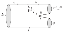
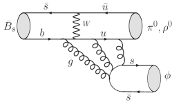
(a) (b) (c)
In order to calculate the two body charmless non-leptonic decays, several attractive QCD-inspired approaches, such as QCD factorization (QCDF) Beneke:1999br ; Beneke:2000ry , perturbative QCD (pQCD) Keum:2000ph ; Lu:2000em and soft-collinear effective theory (SCET) Bauer:2000yr ; Bauer:2001yt , have been proposed in the last decades. In previous studies, the branching fractions of these decays are shown to be about in SM, both in QCDF Beneke:2006hg ; Chang:2017brr ; Cheng:2009mu and in PQCD Ali:2007ff . In the experimental side, the branching fraction of decay has been measured by the LHCb collaboration LHCb:2016vqn ,
| (1) |
with a significance of about . However, the polarization fractions and CPA have not been measured till now. In addition, has been suggested as a tool to measure via the mixing-induced CP asymmetry Fleischer:1994rs . Since in the era of LHCb and Belle-II these two processes become interesting objects for tests of isospin-violation and potential NP Belle-II:2018jsg we will in the following study their phenomenology in full detail, in SM and beyond. In the calculation, we will adopt the QCDF approach, since there is no annihilation contribution in these decays.
Although most experimental data is consistent with the SM predictions, most of us believe that SM is just an effective theory of a more fundamental one yet to be discovered. The presence of a boson associated with an additional gauge symmetry is a well-motivated extension of SM. It should be emphasized that this additional symmetry has not been invented to solve a particular problem of SM, but rather occurs as a byproduct in many models like e.g. grand unified theories, various models of dynamical symmetry breaking and little-Higgs models. An extensive review about the physics of gauge-bosons can be found in Langacker:2008yv . The most interesting feature is that the family non-universal couplings could lead to FCNC in the tree level Buchalla:1995dp ; Nardi:1992nq . The phenomenological effects of in decays have been studied extensively Barger:2009qs ; Cheung:2006tm ; Chang:2009wt ; Hua:2010wf ; Hua:2010we . In this work, we will address the effect of the in the rare decay modes and . Because these two decays are all penguin dominated process and mediated by , they are expected to be sensitive to the effect of the .
The layout of this paper is as follows. In Sec.II we will present the theoretical predictions of and in SM based on QCDF. Sec.III is devoted to the contributions of . Some discussions are also given in this section. We will summarize this work at last.
II Predictions in SM
In SM, the effective weak Hamiltonian mediating FCNC transition of the type has the form Buchalla:1995vs :
| (2) |
where is Fermi coupling constant and is the product of the CKM matrix element. are the Wilson coefficients with the renormalization scale . The are the local four fermion operators, and are the left-handed current-current operators, and are the QCD and electroweak penguin operators, respectively, and they can be expressed as follows:
| (3) |
where and are color indices and are charges of the corresponding quark.
In QCDF approach, the hadronic matrix element of the decay can be written as
| (4) |
where and are the perturbative short-distance interactions and can be calculated perturbatively. are the universal and non-perturbative distribution amplitudes, which can be estimated by the non-perturbative approaches, such as the light cone QCD sum rules, QCD sum rules or lattice QCD.
Because the initial state heavy meson has spin 0, the two vector mesons must have the same helicity due to the conservation of angular momentum. Within the framework of QCDF, the effective Hamiltonian matrix elements are written in the form
| (5) |
where the superscript denotes the helicity of the final-state meson. describes contributions from naive factorization, vertex corrections, penguin contractions and spectator scattering expressed in terms of the flavor operators . Specifically,
| (6) | |||||
where and , and the summation is over . The symbol indicates that the matrix elements of the operators in are to be evaluated in the factorized form.
The decay constant and form factors is defined by Cheng:2009mu :
| (7) | |||||
| (8) | |||||
| (9) | |||||
where , , and
| (10) |
In this work, the form factors of we adopted are from Bharucha:2015bzk based on the light-cone sum rules.
For a decay , its factorizable matrix elements are thus given as
| (11) | |||||
| (12) |
where takes the spectator quark of the meson and is the emitted meson. So, the longitudinal and transverse components are obtained as
| (13) | |||||
| (14) |
In QCDF, in Eq.(6) are basically the Wilson coefficients in conjunction with short-distance nonfactorizable corrections including vertex corrections and hard spectator interactions, and they have the expressions as
| (15) |
where . The upper (lower) signs apply when is odd (even), are the Wilson coefficients, with . The functions stand for vertex corrections, for hard spectator interactions with a hard gluon exchange between the emitted meson and the spectator quark and for penguin contractions. In addition, the expression of the quantities reads
| (18) |
| B meson parameters | ||||||
|---|---|---|---|---|---|---|
| Light vector mensons | ||||||
| Form factors at | ||||||
| Quark masses | ||||||
| Wolfenstein parameters | ||||||
It is noted that there are end-point divergences when we study power corrections in QCDF. When we calculate the hard spectator interactions at twist-3 order, soft and collinear divergences arise from the soft spectator quark Beneke:1999br . Since the treatment of end-point divergences is model dependent, this subleading power corrections generally can be studied only in a phenomenological way. In this work, we shall follow Beneke:1999br ; Beneke:2006hg to model the end-point divergence in as
| (19) |
where is a typical scale, and are the unknown real parameters.
The amplitudes of and decays are written as
| (20) |
| (21) |
We note that the transverse amplitudes are suppressed by a factor relative to , as shown in Eqs.(13) and (14). In addition, the axial-vector and vector contributions to are cancelled by each other in the heavy-quark limit, due to an exact form factor relation Beneke:2000wa . Thus, in quark model Korner:1979ci or naive factorization Kramer:1991xw , the hierarchy of helicity amplitudes
| (22) |
is therefore expected. This hierarchy can also be explained by the chirality flip Kagan:2004uw . The transverse amplitudes defined in the transversity basis are related to the helicity ones via
| (23) |
With the amplitudes, we then obtain the branching fraction of as
| (24) |
where is the lifetime of the meson and is the absolute value of two final-state hadrons’ momentum in the rest frame. Then, three polarization fractions are then defined as
| (25) |
with . In addition, we can also define the direct CPAs as:
| (26) | |||
| (27) |
Using the input parameters listed in Table. 1, we now calculate the branching fractions, polarization fractions and direct CPAs. As aforementioned, two of the most important parameters are and . We firstly follow Beneke:2006hg and adopt the default values and . Three observables of decay and in SM are presented as
| (30) | |||
| (33) | |||
| (36) |
where the errors are from the uncertainties of the nonperturbative parameters. It can be seen that the longitudinal polarization fractions and the CPAs are not sensitive to the nonperturbative inputs, such as decay constants, form factors, and moments in the distribution amplitudes. In addition, we find that for the major uncertainties are from the form factors, while the decay constants dominate the uncertainties in . The branching fractions are in agreement with the previous predictions of Beneke:2006hg , and are larger than those of Cheng:2009mu , because the form factors of we used are larger than theirs. Comparing to the experimental data LHCb:2016vqn shown in Eq. (1), our results is a bit larger than the data. The other observables have not been measured till now.
In ref.Chang:2017brr , the authors had fitted within the all data. Within these ranges, we suppose and obtain the results as
| (39) | |||
| (42) | |||
| (45) |
where the first errors are from the uncertainties of the nonperturbative parameters, and the second ones come from the phase . From the results, it is obvious that the strong phase takes larger uncertainties, especially for decay . Moreover, when the is in the range , the branching fraction of agrees with the data LHCb:2016vqn . In order to show the effects of the parameters , we set and and plot the variations of the branching fractions, CPAs and longitudinal polarization fractions of and decays with the phase in Fig.2 and Fig.3, respectively. In fact, if becomes larger, the uncertainties taken by will be even larger. In all figures, only uncertainties of the form factors (decay constants) in () are considered. In future, if these above observables could be measured with high precision, our theoretical results will be useful for determining the range of in turn.
III Effects of New Physics
| Wilson | ||||
|---|---|---|---|---|
| coefficients | ||||
Though when , the SM prediction of branching fraction of can explain the data, we have chances to search for the effects of NP, because and have not completely confirmed yet. In this section, we will study the effects of an extra gauge boson in these decays . Ignore the mixing between and , we write the couplings of the to fermions as Langacker:2008yv
| (46) |
where is the family index and labels the fermions and . In some string and GUT models Chaudhuri:1994cd ; Cleaver:1998gc ; Cvetic:2001tj ; Cvetic:2002qa ; Kuo:1984gz ; Barger:1987hh , the couplings are not required to be family universal. When rotating to the physical basis, FCNCs generally appear at tree level in both left handed and right handed sectors, explicitly, as
| (47) |
For simplicity, we suppose that the right-handed couplings are flavor-diagonal and . As a result, the part of the effective Hamiltonian for transition has the form as:
| (48) |
where and is the mass. Compared with the effective weak Hamiltonian of SM shown in Eq.(2), the above Hamiltonian Eq. (48) can be rearranged as
| (49) |
where are the effective operators of SM. are the modifications to the corresponding SM Wilson coefficients caused by boson, which are expressed as
| (50) |
in terms of the model parameters at the scale. It is found that the contributes not only to the EW penguins operators but also to the QCD penguins ones. In particular, we suppose that new physics is manifest in the EW penguins by setting as done in Buras:2003dj . Due to the hermiticity of the effective Hamiltonian, the diagonal elements of the effective coupling matrices are real. However, for the off-diagonal one , it could be a complex with a new weak phase . As a result, the resulting contributions to the Wilson coefficients are then written as:
| (51) |
with
| (52) |
The next step is to constrain the ranges of the new defined parameters . In generally, we suppose that both the and gauge groups origin from the same grand unified theories, and is expected. The direct search for boson is one of important physics programs of current and future high-energy colliders. However, the direct signal of the new boson have not been observed in the current experiments such as CMS and ATLAS, implying that the mass of would be larger than the TeV scale. In this work, we set conservatively. Because the family non-universal leads to and FCNC, so that mixing happens at the tree level. Then, the mass difference presents the most strong constraint to the models with boson, and is theoretically required Chang:2009tx ; Li:2012xc ; Barger:2004qc . Meanwhile, in order to explain CPAs of and branching fractions of and , the diagonal elements should satisfy Cheung:2006tm ; Barger:2009qs . In addition this parameter region is of interest for collider detection. Based on the above results obtained, we shall use
| (53) |
We also note that the other SM Wilson coefficients also receive contributions from the boson through renormalization group (RG) evolution. Given that there is no significant RG running effect between and scale, the RG evolution of the modified Wilson coefficients is exactly the same as the ones in the SM Buchalla:1995vs . The Wilson coefficients at and scale have been presented in Table. 2.
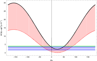
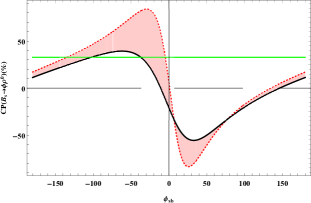
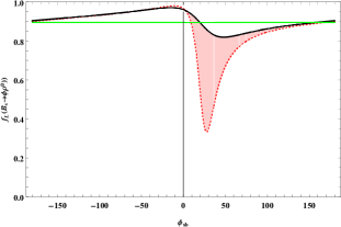
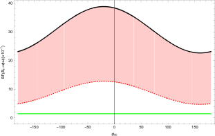
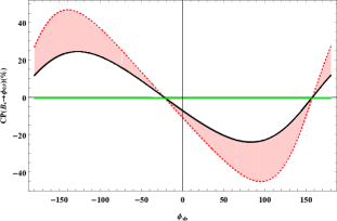

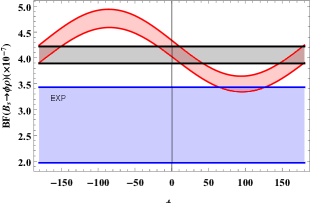
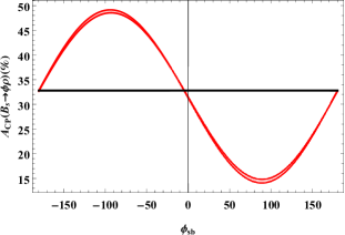
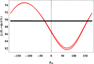
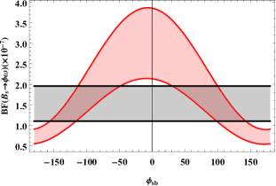
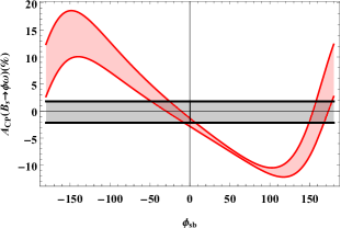
To illustrate the effect of the boson, by setting and , one can get the variations of the CP averaged branching fractions, CPAs and longitudinal polarization fractions of decays and as a function of the new weak phase , as shown in Fig. 4 and Fig. 5, where the horizontal lines are the center values predicted in SM. From left panel of Fig. 4, we find that large , namely a lighter boson, is ruled out. When , is favored. With this range, the branching fraction of would be , which is larger than that of SM by one order of magnitude, as shown in left panel of Fig. 5. As aforementioned, the newly introduced weak phase in the off-diagonal element of plays a major role in changing CPA. The CPAs are much sensitive to and . For , if , the range of CPA is . If , its CPA could reach for some special . The CPA of shares the same characteristics with . These remarkable changes shown in the center panels of Fig. 4 and Fig. 5 will be important signals in testing the model.
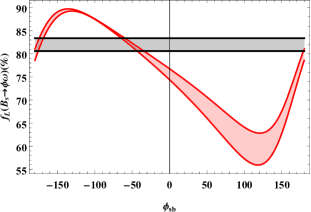
For the decay , the longitudinal polarization fraction is not sensitive to nonperturbative parameters if we adopt and , as shown in the right panel of Fig. 2. When including the contribution of , it could decrease to 0.33, when and . If , it could be enhanced to . For the decay , if , the is in the range , which is larger than the prediction of SM. In addition, we also note that when , the changes is not as remarkable as the case of , which can be seen in the right panels of of Fig. 4 and Fig. 5. The reason is that, when , the contribution of is comparable with that of SM, however when , the contribution of becomes larger than that of SM and dominate the amplitude. If we only consider effect of , for both decays. In future, these observables could be used to probe the effect of new physics. If the were detected in the colliders directly, these decays would also be useful to constrain the couplings.
IV Summary
In this work, we calculated the branching fractions, CP asymmetries and polarization fractions of the decay mode and within the QCD factorization approach in both the SM and the family non-universal model. This approach is suitable because these decay modes have no contributions from annihilation diagrams. In SM, both decays are sensitive to two parameters and , which are from end-point singularities in the hard spectator scattering.
Using the latest results of form factors of , we obtained with , and is with and . These results are a bit larger than the current experimental data. In addition, the longitudinal polarization fraction is and for different values of . Due to the interference between tree and penguin contributions, the CPA is about . The future measurements of and are helpful to determine the parameters (). The decay was also studied.
Because when we adopt , the effects of will be buried in the large uncertainties taken from , we only study its effects in and by setting . In comparison with experimental data, (light ) is ruled out. By setting , the range is favoured. The branching fraction of may be enlarged by one ordr of magnitude by boson within the allowed parameter space. The of decreases to 0.33 with , and reaches to 0.97 with . Furthermore, as the direct CPA is concerned, it can reach with suitable parameter space. The contribution of to was also calculated. All above observables could be measured in the on-going LHC-b experiment and Belle-II, and the future measurements with high precision will provide a plate to test the non-universal model, and can be used to constrain the mass of the boson in turn.
Acknowledgment
This work was supported in part by the National Science Foundation of China under the Grant Nos. 12375089, and the Natural Science Foundation of Shandong province under the Grant No. ZR2022ZD26.
References
- (1) R. L. Workman et al. [Particle Data Group], Review of Particle Physics, PTEP 2022, 083C01 (2022).
- (2) Y. Li and C. D. Lü, Recent Anomalies in B Physics, Sci. Bull. 63, 267-269 (2018) [arXiv:1808.02990 [hep-ph]].
- (3) S. Bifani, S.Descotes-Genon, A.Romero Vidal and M. H. Schune, Review of Lepton Universality tests in decays, J. Phys. G 46, no.2, 023001 (2019) [arXiv:1809.06229 [hep-ex]].
- (4) M. Algueró, A. Crivellin, S. Descotes-Genon, J. Matias and M. Novoa-Brunet, A new -flavour anomaly in : anatomy and interpretation, JHEP 04, 066 (2021) [arXiv:2011.07867 [hep-ph]].
- (5) Y. Li, G. H. Zhao, Y. J. Sun and Z. T. Zou, Family Non-universal Effects on Decays in Perturbative QCD Approach, Phys. Rev. D 106, no.9, 093009 (2022) [arXiv:2209.13389 [hep-ph]].
- (6) T. Kapoor and E. Kou, New physics search via CP observables in decays with left- and right-handed chromomagnetic operators, Phys. Rev. D 108, no.9, 096002 (2023) [arXiv:2303.04494 [hep-ph]].
- (7) M. Beneke, G. Buchalla, M. Neubert and C. T. Sachrajda, QCD factorization for decays: Strong phases and CP violation in the heavy quark limit, Phys. Rev. Lett. 83, 1914-1917 (1999) Phys. Rev. Lett. 83, 1914-1917 (1999) [arXiv:hep-ph/9905312 [hep-ph]].
- (8) M. Beneke, G. Buchalla, M. Neubert and C. T. Sachrajda, QCD factorization for exclusive, nonleptonic B meson decays: General arguments and the case of heavy light final states, Nucl. Phys. B 591, 313-418 (2000) Nucl. Phys. B 591, 313-418 (2000) [arXiv:hep-ph/0006124 [hep-ph]].
- (9) Y. Y. Keum, H. n. Li and A. I. Sanda, Fat penguins and imaginary penguins in perturbative QCD, Phys. Lett. B 504, 6-14 (2001) [arXiv:hep-ph/0004004 [hep-ph]].
- (10) C. D. Lu, K. Ukai and M. Z. Yang, Branching ratio and CP violation of decays in perturbative QCD approach, Phys. Rev. D 63 (2001), 074009 [arXiv:hep-ph/0004213 [hep-ph]].
- (11) A. Ali, G. Kramer, Y. Li, C. D. Lu, Y. L. Shen, W. Wang and Y. M. Wang, Charmless non-leptonic decays to , and final states in the pQCD approach, Phys. Rev. D 76, 074018 (2007) [arXiv:hep-ph/0703162 [hep-ph]].
- (12) C. W. Bauer, S. Fleming, D. Pirjol and I. W. Stewart, An Effective field theory for collinear and soft gluons: Heavy to light decays, Phys. Rev. D 63, 114020 (2001) [arXiv:hep-ph/0011336 [hep-ph]].
- (13) C. W. Bauer, D. Pirjol and I. W. Stewart, Soft collinear factorization in effective field theory, Phys. Rev. D 65, 054022 (2002) [arXiv:hep-ph/0109045 [hep-ph]].
- (14) M. Beneke, J. Rohrer and D. Yang, Branching fractions, polarisation and asymmetries of decays, Nucl. Phys. B 774, 64-101 (2007) [arXiv:hep-ph/0612290 [hep-ph]].
- (15) Q. Chang, X. Li, X. Q. Li and J. Sun, Study of the weak annihilation contributions in charmless decays, Eur. Phys. J. C 77, no.6, 415 (2017) Eur. Phys. J. C 77, no.6, 415 (2017) [arXiv:1706.06138 [hep-ph]].
- (16) H. Y. Cheng and C. K. Chua, QCD Factorization for Charmless Hadronic Decays Revisited, Phys. Rev. D 80, 114026 (2009) Phys. Rev. D 80, 114026 (2009) [arXiv:0910.5237 [hep-ph]].
- (17) R. Aaij et al. [LHCb], Observation of the decay and evidence for , Phys. Rev. D 95, no.1, 012006 (2017) [arXiv:1610.05187 [hep-ex]].
- (18) R. Fleischer, Search for the angle in the electroweak penguin dominated decay , Phys. Lett. B 332, 419-427 (1994)
- (19) E. Kou et al. [Belle-II], The Belle II Physics Book, PTEP 2019, no.12, 123C01 (2019) [arXiv:1808.10567 [hep-ex]].
- (20) P. Langacker, The Physics of Heavy Gauge Bosons, Rev. Mod. Phys. 81, 1199-1228 (2009) [arXiv:0801.1345 [hep-ph]].
- (21) G. Buchalla, G. Burdman, C. T. Hill and D. Kominis, GIM violation and new dynamics of the third generation, Phys. Rev. D 53, 5185-5200 (1996) [arXiv:hep-ph/9510376 [hep-ph]].
- (22) E. Nardi, , new fermions and flavor changing processes. Constraints on models from , Phys. Rev. D 48, 1240-1247 (1993) [arXiv:hep-ph/9209223 [hep-ph]].
- (23) V. Barger, L. L. Everett, J. Jiang, P. Langacker, T. Liu and C. E. M. Wagner, Transitions in Family-dependent Models, JHEP 12, 048 (2009) [arXiv:0906.3745 [hep-ph]].
- (24) K. Cheung, C. W. Chiang, N. G. Deshpande and J. Jiang, Constraints on flavor-changing models by mixing, production, and , Phys. Lett. B 652, 285-291 (2007) [arXiv:hep-ph/0604223 [hep-ph]].
- (25) Q. Chang, X. Q. Li and Y. D. Yang, Constraints on the nonuniversal Z-prime couplings from , and Decays, JHEP 05, 056 (2009) [arXiv:0903.0275 [hep-ph]].
- (26) J. Hua, C. S. Kim and Y. Li, Testing the Non-universal Model in Decay, Phys. Lett. B 690, 508-513 (2010) [arXiv:1002.2532 [hep-ph]].
- (27) J. Hua, C. S. Kim and Y. Li, Annihilation-Type Charmless Radiative Decays of B Meson in Non-universal Model, Eur. Phys. J. C 69, 139-146 (2010) [arXiv:1002.2531 [hep-ph]].
- (28) G. Buchalla, A. J. Buras and M. E. Lautenbacher, Weak decays beyond leading logarithms, Rev. Mod. Phys. 68, 1125-1144 (1996) [arXiv:hep-ph/9512380 [hep-ph]].
- (29) A. Bharucha, D. M. Straub and R. Zwicky, in the Standard Model from light-cone sum rules, JHEP 08, 098 (2016) [arXiv:1503.05534 [hep-ph]].
- (30) M. Beneke and T. Feldmann, Symmetry breaking corrections to heavy to light B meson form-factors at large recoil, Nucl. Phys. B 592, 3-34 (2001) [arXiv:hep-ph/0008255 [hep-ph]].
- (31) J. G. Korner and G. R. Goldstein, Quark and Particle Helicities in Hadronic Charmed Particle Decays, Phys. Lett. B 89, 105-110 (1979)
- (32) G. Kramer and W. F. Palmer, Branching ratios and CP asymmetries in the decay , Phys. Rev. D 45, 193-216 (1992)
- (33) A. L. Kagan, Polarization in decays, Phys. Lett. B 601, 151-163 (2004) [arXiv:hep-ph/0405134 [hep-ph]].
- (34) S. Chaudhuri, S. W. Chung, G. Hockney and J. D. Lykken, String consistency for unified model building, Nucl. Phys. B 456, 89-129 (1995) [arXiv:hep-ph/9501361 [hep-ph]].
- (35) G. Cleaver, M. Cvetic, J. R. Espinosa, L. L. Everett, P. Langacker and J. Wang, Physics implications of flat directions in free fermionic superstring models 1. Mass spectrum and couplings, Phys. Rev. D 59, 055005 (1999) [arXiv:hep-ph/9807479 [hep-ph]].
- (36) M. Cvetic, G. Shiu and A. M. Uranga, Three family supersymmetric standard - like models from intersecting brane worlds, Phys. Rev. Lett. 87, 201801 (2001) [arXiv:hep-th/0107143 [hep-th]].
- (37) M. Cvetic, P. Langacker and G. Shiu, Phenomenology of a three family standard like string model, Phys. Rev. D 66, 066004 (2002) [arXiv:hep-ph/0205252 [hep-ph]].
- (38) T. K. Kuo and N. Nakagawa, An extension of the electroweak theory, Phys. Rev. D 30, 2011 (1984)
- (39) V. D. Barger, N. G. Deshpande, T. Kuo, A. Bagneid, S. Pakvasa and K. Whisnant, Discovery Limits of New Gauge Bosons of , Int. J. Mod. Phys. A 2, 1327 (1987)
- (40) A. J. Buras, R. Fleischer, S. Recksiegel and F. Schwab, , new physics in and implications for rare and decays, Phys. Rev. Lett. 92, 101804 (2004) Phys. Rev. Lett. 92, 101804 (2004) [arXiv:hep-ph/0312259 [hep-ph]].
- (41) V. Barger, C. W. Chiang, J. Jiang and P. Langacker, mixing in models with flavor-changing neutral currents, Phys. Lett. B 596, 229-239 (2004) [arXiv:hep-ph/0405108 [hep-ph]].
- (42) Q. Chang, X. Q. Li and Y. D. Yang, Family Non-universal effects on mixing, and Decays, JHEP 02, 082 (2010) [arXiv:0907.4408 [hep-ph]].
- (43) X. Q. Li, Y. M. Li, G. R. Lu and F. Su, mixing in a family non-universal model revisited, JHEP 05, 049 (2012) [arXiv:1204.5250 [hep-ph]].