Signal of phase transition hidden in quasinormal modes of regular AdS black holes

Yang Guo, Hao Xie, and Yan-Gang Miao

School of Physics, Nankai University, Tianjin 300071, China

We discuss the intrinsic relations between thermodynamic phase transitions and quasinormal modes in regular AdS black holes, specifically in the Bardeen and Hayward AdS classes. To this end, we calculate the quasinormal modes of massless scalar field perturbations around small and large black holes via the Horowitz-Hubeny method. By investigating the isobaric and isothermal phase transitions for Bardeen and Hayward AdS black holes in detail, we observe that a dramatic change of quasinormal modes appears near the phase transition point of small and large black holes, and that it corresponds to the swallow tail structure in the plane of Gibbs free energy and pressure. Moreover, by analyzing the evolution of black holes along the coexistence curve of small and large black hole phases, we also observe the dramatic change in quasinormal modes. Such a phenomenon confirms the signal of the phase transition in the quasinormal mode spectrum, which can be understood as a thermodynamic signal hidden in the dynamical spectrum.

1 Introduction

Quasinormal modes have been studied [1, 2, 3, 4, 5, 6] in a wide range of issues in General Relativity and alternative theories of gravity. In general, quasinormal modes are used to describe the stability of black holes perturbed by an external field or by a spacetime metric, and they are also thought to carry the information of gravitational waves.

There have been some arguments [7, 8] about whether black holes carry thermodynamic information that might be observed in future. In addition, it has been suggested [9] that scalar field perturbations are related to thermodynamic phase transitions of charged black holes, where an obvious change of quasinormal modes may be associated with a second order phase transition. Furthermore, some studies have pointed out [7, 10] that a phase transition would probably connect to quasinormal modes, but their correspondence between the thermodynamic and dynamic aspects should be analyzed in more details instead of simply by numerical coincidence.

Recently, a remarkable progress has been made [11, 12, 13, 14], indicating that the information of phase transitions does appear in the quasinormal mode spectra only for some specific cases in singular black holes. It has been expected for a long time that thermodynamic phase transitions of black holes have some observational characteristics, which would be possible if the phase transitions have the connections to quasinormal modes. In the present work, we deal with this issue for regular black holes through the procedure of phase transitions. In terms of the analyses [15, 16, 17, 18] of thermodynamic phase transitions for AdS black holes, we use the semi-analytical method proposed [19] by Horowitz and Hubeny to compute the quasinormal modes for two regular AdS black holes, the Bardeen and Hayward AdS classes, and then investigate the corresponding relations between thermodynamic phase transitions and quasinormal modes. In the thermodynamic aspect, we analyze the isobaric and isothermal phase transitions of small-large black holes in an extended phase space by showing the swallow tail structure in the plane of Gibbs free energy and pressure, and also discuss the evolution of black holes along the coexistence curve of small and large black hole phases. On the other hand, in the dynamic aspect, we calculate the quasinormal modes of massless scalar field perturbations around small and large Bardeen and Hayward AdS black holes via the Horowitz-Hubeny method. By connecting the two aspects, we indeed find the signal of the phase transition in the quasinormal mode spectrum for Bardeen and Hayward AdS black holes.

Our paper is organized as follows. In Sec. 2.1, we make a general introduction to Einstein gravity coupled with nonlinear electrodynamics, and then analyze thermodynamic phase transitions in regular AdS black holes in Sec. 2.2. Next, we introduce the massless scalar field perturbation in an asymptotic AdS spacetime in terms of the Horowitz-Hubeny method in Sec. 3.1. We compute the quasinormal modes of scalar field perturbations when the Bardeen and Hayward AdS black holes undergo the isobaric and isothermal phase transitions in Sec. 3.2 and Sec. 3.3, respectively. In Sec. 3.4, we calculate quasinormal modes when the two black holes evolve along the coexistence curves, and analyze the behavior of quasinormal modes near the phase transition point of small-large black holes. Finally, we give our conclusions in Sec. 4.

2 Phase transition in regular AdS black holes

2.1 Einstein gravity coupled with nonlinear electrodynamics

The Einstein gravity theory coupled with a nonlinear electromagnetic field is described by the action,

$$S=\frac{1}{16\pi}\int d^{4}x\sqrt{-g}\left({R}-2\Lambda-\mathcal{L}(F)\right),$$ (2.1)

where $R$ is scalar curvature and $F=\frac{1}{4}F^{ab}F_{ab}$ the electromagnetic invariant in the four-dimensional spacetime with indices $a$ and $b$. And the Lagrangian density of nonlinear electrodynamics is given [20] by

$$\mathcal{L}(F)=\frac{4\mu M\left(2Fq^{2}\right)^{(\nu+3)/4}}{q^{3}\left[1+\left(2Fq^{2}\right)^{\nu/4}\right]^{(\mu+\nu)/\nu}},$$ (2.2)

which yields the static and spherically symmetric solution with the following shape function,

$$f(r)=1-\frac{2Mr^{\mu-1}}{(r^{\nu}+q^{\nu})^{\mu/\nu}}+\frac{r^{2}}{l^{2}},$$ (2.3)

where $M$ denotes the black hole mass, $q$ the magnetic charge, $l$ the radius of AdS spacetime, and $\mu$ and $\nu$ the dimensionless constants which characterize the nonlinear degree of electromagnetic fields. For the case of $\mu=3$ and $\nu=2$, this solution reduces [21] to the Bardeen AdS black hole, and for the case of $\mu=\nu=3$, it reduces [22] to the Hayward AdS black hole. The first law of thermodynamics can be written [23, 24, 25] in the form,

$$dM=\frac{\kappa}{8\pi}dA+\Psi dq+K_{q}dq+K_{M}dM,$$ (2.4)

where $\Psi$ is the magnetic potential, and $K_{q}$ and $K_{M}$ appear as the factors of the extra terms $K_{q}dq$ and $K_{M}dM$,

$$\Psi = \frac{M\left\{\mu q^{\nu}r_{+}^{-\nu}+3\left(1+q^{\nu}r_{+}^{-\nu}\right)\left[\left(1+q^{\nu}r_{+}^{-\nu}\right)^{\mu/\nu}-1\right]\right\}}{2q\left(1+q^{\nu}r_{+}^{-\nu}\right)^{(\mu+\nu)/\nu}},$$ (2.5)

$$K_{q} = \frac{Mr_{+}^{\mu}\left[3-3\left(q^{\nu}r_{+}^{-\nu}+1\right)^{\mu/\nu}+\mu q^{\nu}(r_{+}^{\nu}+q^{\nu})^{-1}\right]}{2q\left(r_{+}^{\nu}+q^{\nu}\right)^{\mu/\nu}},$$ (2.6)

$$K_{M} = 1-\frac{r_{+}^{\mu}}{\left(r_{+}^{\nu}+q^{\nu}\right)^{\mu/\nu}}.$$ (2.7)

Here $r_{+}$ stands for the radius of outer horizons as usual.

2.2 The small-large black hole phase transition

2.2.1 Bardeen AdS black holes

The first law, see Eq. (2.4) together with the term $VdP$ owing to the introduction of the AdS spacetime, can be rearranged to be a “standard form”, i.e. the formulation without the extra terms mentioned above, as follows:

$$dM=T^{\prime}dS+V^{\prime}dP+\Psi^{\prime}dq,$$ (2.8)

where the effective temperature $T^{\prime}$, effective volume $V^{\prime}$ and effective magnetic potential $\Psi^{\prime}$ are defined by

$$T^{\prime}\equiv\frac{T}{1-K_{M}},\qquad V^{\prime}\equiv\frac{V}{1-K_{M}},\qquad\Psi^{\prime}\equiv\frac{\Psi+K_{q}}{1-K_{M}}.$$ (2.9)

For Bardeen AdS black holes with $\mu=3$ and $\nu=2$, by using Eqs. (2.5), (2.6), (2.7), and (2.9) we obtain

$$T^{\prime} = \frac{\sqrt{q^{2}+r_{+}^{2}}\left(8\pi Pr_{+}^{4}-2q^{2}+r_{+}^{2}\right)}{4\pi r_{+}^{4}},$$ (2.10)

$$V^{\prime} = \frac{4}{3}\pi\left(q^{2}+r_{+}^{2}\right)^{3/2},$$ (2.11)

$$\Psi^{\prime} = \frac{3Mq}{q^{2}+r_{+}^{2}}.$$ (2.12)

In the extended phase space, $(T^{\prime},P,\Psi^{\prime};S,V^{\prime},q)$, the Gibbs free energy takes the form,

$$G^{\prime}=M-T^{\prime}S,$$ (2.13)

and correspondingly the equation of state reads from Eqs. (2.10) and (2.11),

$$P=P(T^{\prime},V^{\prime})=\frac{4\pi T^{\prime}\left(\frac{3V^{\prime}}{4\pi}-q^{3}\right)^{4/3}+3q^{3}-\frac{3V^{\prime}}{4\pi}}{8\pi\left(\frac{3V^{\prime}}{4\pi}-q^{3}\right)^{5/3}}.$$ (2.14)

Substituting Eqs. (2.10), (2.11), and (2.14) into the following critical condition,

$$\left(\frac{\partial P}{\partial V^{\prime}}\right)_{T^{\prime}}=0,\qquad\left(\frac{\partial^{2}P}{\partial V^{\prime 2}}\right)_{T^{\prime}}=0,$$ (2.15)

we can solve the critical point,

$$T^{\prime}_{c} = \frac{5\sqrt{188\sqrt{10}-505}}{432\pi q},$$

$$V^{\prime}_{c} = \frac{4}{3}\left(2\sqrt{10}+5\right)^{3/2}\pi q^{3},$$

$$P_{c} = \frac{5\sqrt{10}-13}{432\pi q^{2}},$$ (2.16)

at which the phase transition of small and large black holes goes to the end in the evolution of the Bardeen AdS class, see Sec. 3.4, for the details.

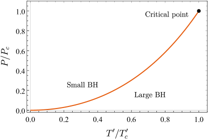
Figure 1: The coexistence curve of small-large phases for Bardeen AdS black holes

Fig. 1 clearly shows the existence of phase transitions of small and large black holes in the Bardeen AdS class, where the coexistence curve given by the Gibbs free energy Eq. (2.13) obeys strictly the Maxwell law in the extended phase space, $(T^{\prime},P,\Psi^{\prime};S,V^{\prime},q)$. The curve describes coexistence of small and large black holes when the phase transition occurs. The critical point is highlighted by black color at the end of the coexistence curve. From this figure, we can see that the effective temperature and pressure of the small black hole phase are strictly the same as those of large black hole phase.

2.2.2 Hayward AdS black holes

As discussed for the Bardeen AdS class, we derive the following effective quantities by using Eqs. (2.4)-(2.9) with $\mu=\nu=3$ for the Hayward AdS class,

$$T^{\prime} = \frac{8\pi Pr_{+}^{5}-2q^{3}+r_{+}^{3}}{4\pi r_{+}^{4}},$$

$$V^{\prime} = \frac{4}{3}\pi\left(q^{3}+r_{+}^{3}\right),$$

$$\Psi^{\prime} = \frac{3Mq^{2}r_{+}^{3}}{(r_{+}^{3}+q^{3})^{2}}.$$ (2.17)

Corresponding, we obtain the critical point of phase transitions,

$$T^{\prime}_{c} = \frac{3}{8\sqrt[3]{20}\pi q},$$

$$V^{\prime}_{c} = 28\pi q^{3},$$

$$P_{c} = \frac{3}{80\sqrt[3]{50}\pi q^{2}}.$$ (2.18)

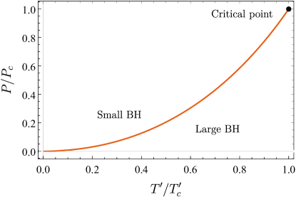
Figure 2: The coexistence curve of small-large phases for Hayward AdS black holes

Fig. 2 depicts the coexistence curve of small and large black hole phases in the Hayward AdS class, where the critical point is highlighted by black color at the end of the coexistence curve. Similarly, the effective temperature and pressure of small black holes are the same as those of large black holes when the phase transition occurs.

3 Signal of phase transition hidden in quasinormal modes

3.1 Perturbation in an asymptotic AdS spacetime

Now we introduce the Horowitz-Hubeny method [19] for a scalar field perturbation in an asymptotic AdS spacetime. A massless scalar field is described by the equation,

$${\nabla}^{2}\Phi=0,$$ (3.19)

and it is usually decomposed by the following form in a spherically symmetric spacetime,

$$\Phi(t,r,\theta,\phi)=\frac{1}{r}\psi(r)Y(\theta,\phi)e^{-i\omega t},$$ (3.20)

where $Y(\theta,\phi)$ is spherical harmonics. Using the tortoise coordinate defined by $dr_{*}=dr/f(r)$, we derive the radial equation,

$$\frac{d^{2}\psi}{{dr_{*}}^{2}}+(\omega^{2}-V)\psi=0,$$ (3.21)

where the potential takes the form for the metric with the shape function Eq. (2.3),

$$V(r)=f(r)\left[\frac{l(l+1)}{r^{2}}+\frac{1}{r}f^{\prime}(r)\right].$$ (3.22)

In an asymptotically flat spacetime, the potential vanishes at infinity. Therefore, the quasinormal modes are determined by the outgoing waves near infinity, $\Phi\sim e^{-i\omega(t-r_{*})}$, and by the ingoing waves near an outer horizon, $\Phi\sim e^{-i\omega(t+r_{*})}$. However, the situation is different in an asymptotic AdS spacetime, where the potential diverges at infinity and thus the wave function $\Phi$ vanishes. As a result, the quasinormal modes related to an AdS spacetime are determined only by ingoing waves near an outer horizon. To this end, we calculate the modes of ingoing waves near an outer horizon, $\Phi\sim e^{-i\omega(t+r_{*})}$, and write [19] the line element in the ingoing Eddington coordinates for the sake of convenience,

$$ds^{2}=-f(r)dv^{2}+2dvdr+r^{2}d\Omega^{2}.$$ (3.23)

By using the corresponding decomposition of $\Phi$,

$$\Phi(v,r,\theta,\phi)=\frac{1}{r}\psi(r)Y(\theta,\phi)e^{-i\omega v},$$ (3.24)

and substituting it into Eq. (3.19), we derive the following radial equation,

$$f(r)\frac{d^{2}\psi(r)}{dr^{2}}+[f^{\prime}(r)-2i\omega]\frac{\psi(r)}{r}-V(r)\psi(r)=0,$$ (3.25)

where the effective potential $V(r)$ is expressed by

$$V(r)=\frac{1}{r}f^{\prime}(r)+\frac{l(l+1)}{r^{2}}.$$ (3.26)

In order to calculate the quasinormal modes, we expand the solution in a power series at the horizon $r_{+}$ and restrict the solution to zero at infinity. The range of our solution is $r_{+}<r<+\infty$. In order to give the quasinormal modes numerically, we change the range to a finite one by setting $x=1/r$, and thus transfer Eq. (3.25) into the following form,

$$s(x)\frac{d^{2}\psi(x)}{dx^{2}}+\frac{t(x)}{x-x_{+}}\frac{d\psi(x)}{dx}+\frac{u(x)}{(x-x_{+})^{2}}\psi(x)=0,$$ (3.27)

where $x_{+}=1/r_{+}$ and the three coefficient functions take the forms,

$$s(x) =-\frac{x^{4}f(x)}{x-x_{+}},$$ (3.28)

$$t(x) =-2x^{3}f(x)-x^{4}\frac{df(x)}{dx}-2i\omega x^{2},$$ (3.29)

$$u(x) =(x-x_{+})V(x).$$ (3.30)

We can expand them as the Taylor series with the center at $x=x_{+}$,

$$s(x)=\sum_{n=0}^{\infty}s_{n}(x-x_{+})^{n},$$

$$t(x)=\sum_{n=0}^{\infty}t_{n}(x-x_{+})^{n},$$

$$u(x)=\sum_{n=0}^{\infty}u_{n}(x-x_{+})^{n}.$$ (3.31)

It is worth noting that $s_{0}=2x_{+}^{2}\kappa$, $t_{0}=2x_{+}^{2}(\kappa-i\omega)$, and $u_{0}=0$ at the horizon $x=x_{+}$, where $\kappa$ is the surface gravity and can be expressed as $\kappa=f^{\prime}(r_{+})/2$. To determine the behavior of the quasinormal modes near the horizon, we set the solution $\psi(x)$ as

$$\psi(x)=\sum_{n=0}^{\infty}a_{n}(x-x_{+})^{n}.$$ (3.32)

When substituting Eq. (3.31) and Eq. (3.32) into Eq. (3.27), we obtain the recursion relations of $a_{n}$,

$$a_{n}=-\frac{1}{P_{n}}\sum_{k=0}^{n-1}\left[k(k-1)s_{n-k}+kt_{n-k}+u_{n-k}\right]a_{k},$$ (3.33)

where $P_{n}$ is given by

$$P_{n}=n(n-1)s_{0}+nt_{0}=2x_{+}^{2}n(n\kappa-i\omega).$$ (3.34)

Since the solution $\psi(x)$ satisfies the boundary condition: $\psi(x)\rightarrow 0$ in the limit of $x\rightarrow 0$, we need to find the zeros of the equation, $\sum_{n=0}^{\infty}a_{n}(\omega)(-x_{+})^{n}=0$, in the complex $\omega$ plane. As a result, we compute the complex quasinormal frequencies by truncating the series, $\sum_{n=0}^{\infty}a_{n}(\omega)(-x_{+})^{n}$, at a large enough value of $n$ and computing the relevant finite sum as a function of $\omega$. In the following subsections, we calculate the quasinormal frequencies to the order of $n=50$ and obtain the convergent numerical results, where our investigation follows the procedures of isobaric and isothermal phase transitions in Sec. 3.2 and Sec. 3.3, respectively, and also the evolution procedure along coexistence curves of small-large black hole phases in Sec. 3.4.

3.2 Isobaric phase transition

When the effective temperature goes large, the Bardeen and Hayward AdS black holes evolve and cross the coexistence curve along the isobar as shown in Fig. 3, where the arrow indicates the direction of small-large black hole phase transition, that is, the small black hole phase passes through the phase transition point of the coexistence curve and then turns into the large black hole phase.

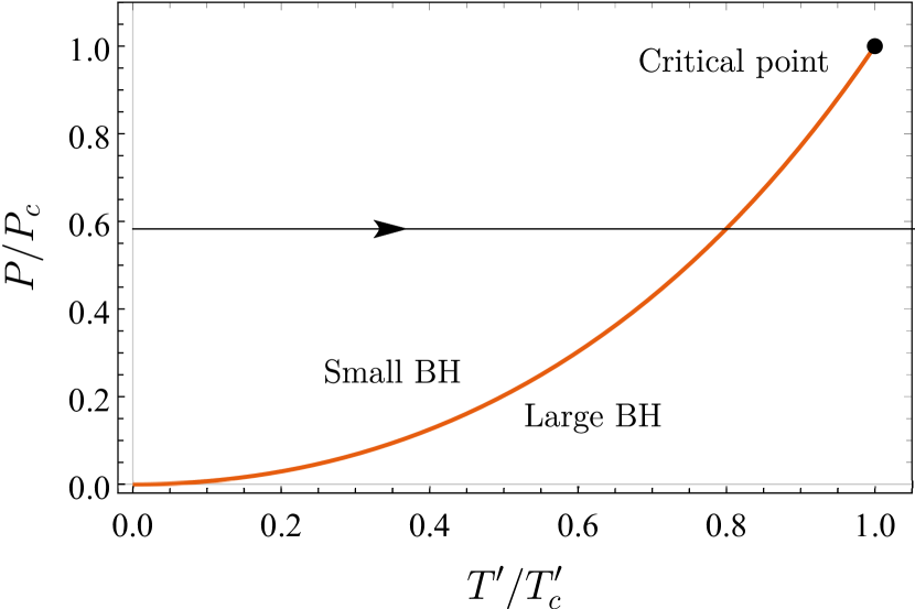
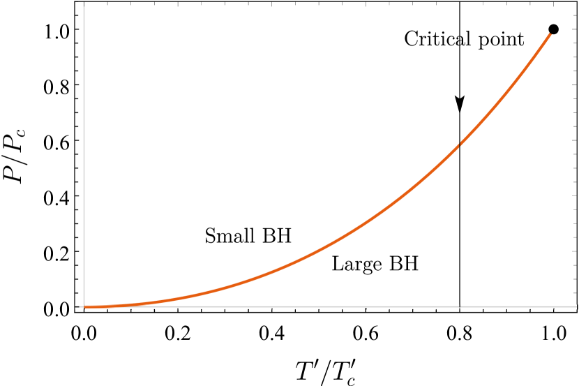
(a) Bardeen AdS black hole

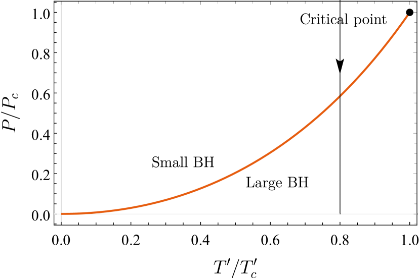
(b) Hayward AdS black hole

Figure 3: Isobaric phase transition and coexistence curve for small and large black holes

Next, we calculate the quasinormal modes when the Bardeen and Hayward AdS black holes evolve along this isobar shown in Fig. 3, and list the numerical results of quasinormal mode frequencies for both the Bardeen and Hayward AdS classes in Table 1. For each class, the upper part, above the horizontal line, gives the data for the small black hole phase, while the lower part does for the large black hole phase. Specifically, the isobar $P=0.00483$ or $P=0.00757$ is set for Bardeen or Hayward AdS black holes. When the effective temperature of small black holes increases and reaches the value at which the small-large black hole phase transition occurs, $T^{\prime}_{0}=0.05577$ for the Bardeen AdS class and $T^{\prime}_{0}=0.07036$ for the Hayward AdS class, respectively, a dramatic change appears in quasinormal spectra.

Bardeen AdS black hole
$T^{\prime}$	$r_{+}$	$\omega$
0.050	0.915	2.35954 - 3.60483 i
0.051	0.927	2.37202 - 3.62750 i
0.052	0.941	2.38627 - 3.65313 i
0.053	0.956	2.40127 - 3.68049 i
0.054	0.974	2.41947 - 3.71606 i
0.055	0.994	2.43878 - 3.75648 i
0.056	3.442	6.47910 - 9.38757 i
0.057	3.699	6.94789 - 10.0555 i
0.058	3.920	7.35130 - 10.6318 i
0.059	4.119	7.71520 - 11.1521 i
0.060	4.304	8.05349 - 11.6366 i
Hayward AdS black hole
$T^{\prime}$	$r_{+}$	$\omega$
0.065	0.816	2.55852 - 2.91317 i
0.066	0.825	2.56397 - 2.92913 i
0.067	0.835	2.56989 - 2.94712 i
0.068	0.846	2.57623 - 2.96714 i
0.069	0.858	2.58288 - 2.98917 i
0.070	0.871	2.58983 - 3.01316 i
0.071	2.888	5.68775 - 7.75504 i
0.072	3.044	5.96104 - 8.16489 i
0.073	3.183	6.20559 - 8.53076 i
0.074	3.311	6.43156 - 8.86816 i
0.075	3.431	6.64403 - 9.18482 i

Table 1: The quasinormal mode frequencies of a massless scalar field perturbation with respect to the effective temperature $T^{\prime}$, where the isobar $P=0.00483$ or $P=0.00757$ is set for Bardeen or Hayward AdS black holes. The phase transition point is located at $T^{\prime}_{0}=0.05577$ for Bardeen AdS black holes, or $T^{\prime}_{0}=0.07036$ for Hayward AdS black holes.

3.3 Isothermal phase transition

When the pressure becomes small, the Bardeen and Hayward AdS black holes evolve and cross the coexistence curve along the isotherm as shown in Fig. 4, where the arrow indicates the direction of small-large black hole phase transition, that is, the small black hole phase passes through the phase transition point of the coexistence curve and then turns into the large black hole phase.

(a) Bardeen AdS black hole

(b) Hayward AdS black hole

Figure 4: Isothermal phase transition and coexistence curve for small and large black holes

Next, we calculate the quasinormal modes when the Bardeen and Hayward AdS black holes evolve along this isotherm shown in Fig. 4, and list the numerical results of quasinormal mode frequencies for both the Bardeen and Hayward AdS classes in Table 2. For each class, the upper part, above the horizontal line, gives the data for the small black hole phase, while the lower part does for the large black hole phase. Specifically, the isotherm $T^{\prime}=0.8T^{\prime}_{c}$ is set for both Bardeen and Hayward AdS black holes. When the pressure of small black holes decreases and reaches the value at which the small-large black hole phase transition occurs, $P_{0}=0.00483$ for the Bardeen AdS class and $P_{0}=0.00757$ for the Hayward AdS class, respectively, a dramatic change appears in quasinormal spectra.

Combining the results in the above subsection with those in this one, we can conclude that the same phenomenon exists, i.e., the dramatic change of quasinormal modes appears in both the isobaric and isothermal phase transitions.

Bardeen AdS black hole
$P$	$r_{+}$	$\omega$
0.0053	0.988	2.43274 - 3.74402 i
0.0052	0.993	2.43791 - 3.75502 i
0.0051	0.997	2.44169 - 3.76321 i
0.0050	1.002	2.44628 - 3.77294 i
0.0049	1.008	2.45140 - 3.78524 i
0.0048	3.443	6.48103 - 9.39022 i
0.0047	3.639	6.83841 - 9.89935 i
0.0046	3.829	7.18522 - 10.3943 i
0.0045	4.015	7.52490 - 10.8800 i
0.0044	4.202	7.86690 - 11.3693 i
0.0043	4.390	8.21091 - 11.8621 i
Hayward AdS black hole
$P$	$r_{+}$	$\omega$
0.0080	0.866	2.58719 - 3.00396 i
0.0079	0.868	2.58825 - 3.00760 i
0.0078	0.871	2.58983 - 3.01316 i
0.0077	0.873	2.59087 - 3.01684 i
0.0076	0.876	2.59240 - 3.02232 i
0.0075	2.848	5.61789 - 7.65011 i
0.0074	2.948	5.79271 - 7.91257 i
0.0073	3.045	5.96280 - 8.16752 i
0.0072	3.141	6.13160 - 8.42015 i
0.0071	3.236	6.29907 - 8.67041 i
0.0070	3.331	6.46693 - 8.92091 i

Table 2: The quasinormal mode frequencies of a massless scalar field perturbation with respect to the pressure $P$, where the isotherm $T^{\prime}=0.8T^{\prime}_{c}$ is set for both Bardeen and Hayward AdS black holes. The phase transition point is located at $P_{0}=0.00483$ for Bardeen AdS black holes, or $P_{0}=0.00757$ for Hayward AdS black holes.

3.4 Quasinormal modes on coexistence curves

In Sec. 3.2 and Sec. 3.3, we investigate the isobaric and isothermal phase transitions for both Bardeen and Hayward AdS black holes and find that the dramatic changes of quasinormal modes indeed indicate the signal of phase transitions. In this subsection, we analyze the thermodynamic and dynamic behaviors of the two regular AdS black holes when the evolution of the black holes goes along the coexistence curves as shown in Fig. 5, where the arrow shows the evolution direction of the black holes towards the critical points.

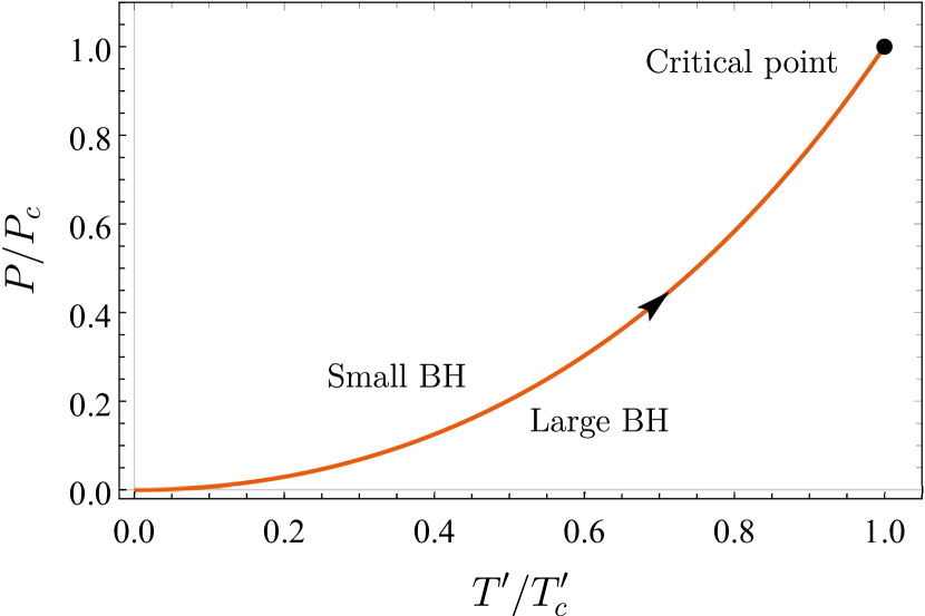
(a) Bardeen AdS black hole

(b) Hayward AdS black hole

Figure 5: Coexistence curve for small and large black holes

As known, when a phase transition occurs in an AdS black hole, the Gibbs free energy of this black hole exhibits the swallow tail structure as shown in Fig. 6, which corresponds to an intermediate state of phase transitions. In our case of Bardeen and Hayward AdS classes, this intermediate state means that the small and large black holes coexist. When the critical point is reached, see the purple curve in Fig. 6, the small-large black hole phase transition ends and then both the intermediate state and the swallow tail structure of the Gibbs free energy disappear simultaneously.

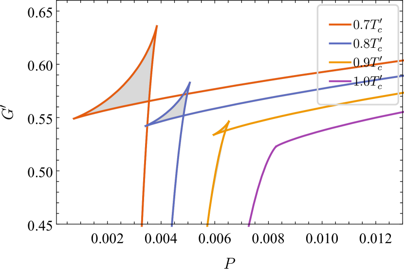
(a) Bardeen AdS black hole

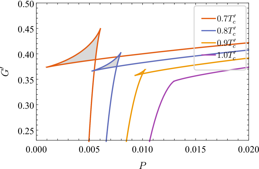
(b) Hayward AdS black hole

Figure 6: The swallow tail structure of Gibbs free energy

By calculating those quasinormal modes that the Bardeen and Hayward AdS black holes evolve along the coexistence curves, we find from Fig. 7 and Fig. 8 that the differences between small and large black holes’ real (imaginary) parts are very dramatic when the black holes stay at the point of coexistence curves far away from the critical point, and that such a difference gradually decreases when the point moves towards the critical point and vanishes at the critical point. Moreover, the shaded area in the swallow tail structure of Gibbs free energy, see Fig. 6, corresponds to the shaded area associated with quasinormal modes, see Fig. 7 and Fig. 8, and both areas disappear at the critical point of phase transitions. As a result, the dynamic behavior of small-large black hole coexistence confirms the signal of thermodynamic phase transitions from an alternative viewpoint that is different from isobaric and isothermal phase transitions.

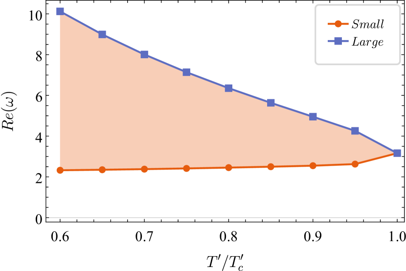
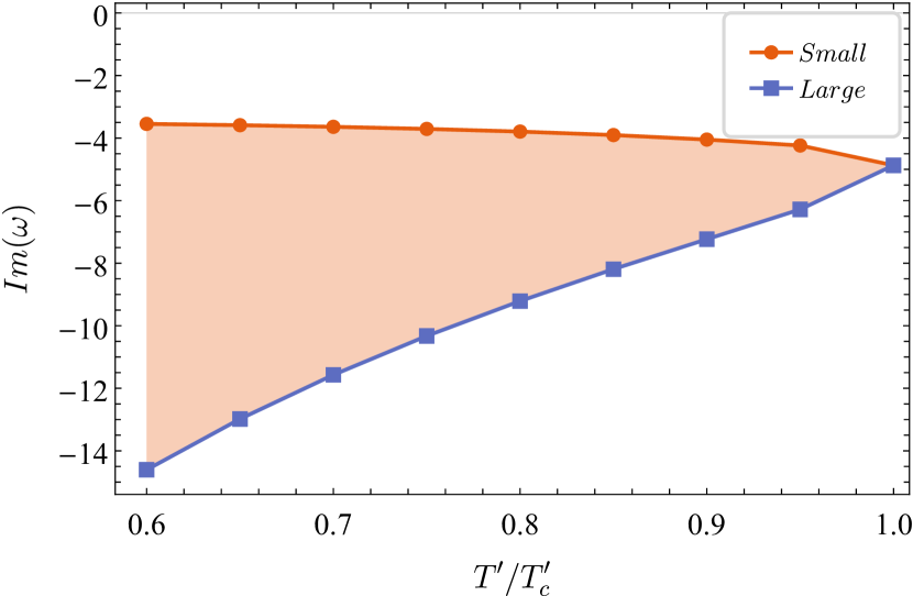
Figure 7: Quasinormal modes when the Bardeen AdS black holes evolve along the coexistence curves

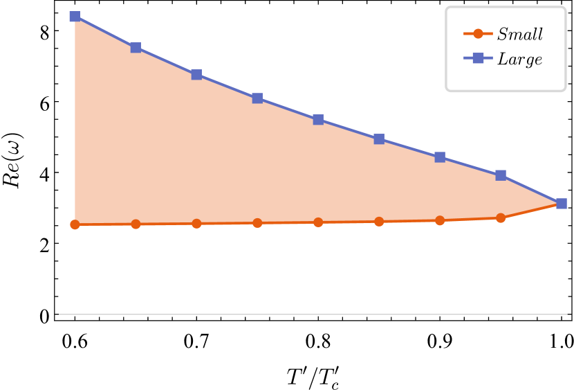
Figure 8: Quasinormal modes when the Hayward AdS black holes evolve along the coexistence curves

4 Summary

In the present work, we investigate systematically the correlation between phase transitions and quasinormal modes for regular AdS black holes by following the procedures of isobaric and isothermal phase transitions and the evolution procedure along coexistence curves of small-large black hole phases, where the phase transitions belong to thermodynamics, while the quasinormal modes dynamics. As expected, we confirm that such a correlation is inevitable but not accidental by numerical coincidence. We thus conclude that quasinormal modes can be a dynamic probe of thermodynamic phase transitions, which implies that the information of phase transitions may be hidden in the observations of gravitational waves that are closely related to quasinormal modes.

Acknowledgments

This work was supported in part by the National Natural Science Foundation of China under Grant No. 12175108.

References

- [1] E. Berti and K.D. Kokkotas, Quasinormal modes of Reissner-Nordström-anti-de Sitter black holes: Scalar, electromagnetic and gravitational perturbations, Phys. Rev. D 67 (2003) 064020 [gr-qc/0301052].
- [2] R.A. Konoplya, Quantum corrected black holes: quasinormal modes, scattering, shadows, Phys. Lett. B 804 (2020) 135363 [1912.10582].
- [3] Y. Guo and Y.-G. Miao, Null geodesics, quasinormal modes and the correspondence with shadows in high-dimensional Einstein-Yang-Mills spacetimes, Phys. Rev. D 102 (2020) 084057 [2007.08227].
- [4] Y. Guo, C. Lan and Y.-G. Miao, Bounce corrections to gravitational lensing, quasinormal spectral stability, and gray-body factors of Reissner-Nordström black holes, Phys. Rev. D 106 (2022) 124052 [2201.02971].
- [5] E. Berti, V. Cardoso and A.O. Starinets, Quasinormal modes of black holes and black branes, Class. Quant. Grav. 26 (2009) 163001 [0905.2975].
- [6] R.A. Konoplya and A. Zhidenko, Quasinormal modes of black holes: From astrophysics to string theory, Rev. Mod. Phys. 83 (2011) 793 [1102.4014].
- [7] E. Berti and V. Cardoso, Quasinormal modes and thermodynamic phase transitions, Phys. Rev. D 77 (2008) 087501 [0802.1889].
- [8] Y. Liu, D.-C. Zou and B. Wang, Signature of the Van der Waals like small-large charged AdS black hole phase transition in quasinormal modes, JHEP 09 (2014) 179 [1405.2644].
- [9] J. Jing and Q. Pan, Quasinormal modes and second order thermodynamic phase transition for Reissner-Nordstrom black hole, Phys. Lett. B 660 (2008) 13 [0802.0043].
- [10] X.-P. Rao, B. Wang and G.-H. Yang, Quasinormal modes and phase transition of black holes, Phys. Lett. B 649 (2007) 472 [0712.0645].
- [11] B. Wang, C.-Y. Lin and E. Abdalla, Quasinormal modes of Reissner-Nordstrom anti-de Sitter black holes, Phys. Lett. B 481 (2000) 79 [hep-th/0003295].
- [12] J. Shen, B. Wang, C.-Y. Lin, R.-G. Cai and R.-K. Su, The phase transition and the Quasi-Normal Modes of black Holes, JHEP 07 (2007) 037 [hep-th/0703102].
- [13] Y.S. Myung, Phase transition for black holes with scalar hair and topological black holes, Phys. Lett. B 663 (2008) 111 [0801.2434].
- [14] G. Koutsoumbas, E. Papantonopoulos and G. Siopsis, Phase Transitions in Charged Topological-AdS Black Holes, JHEP 05 (2008) 107 [0801.4921].
- [15] D. Kubiznak and R.B. Mann, P-V criticality of charged AdS black holes, JHEP 07 (2012) 033 [1205.0559].
- [16] Z.-M. Xu, Y.-S. Wang, B. Wu and W.-L. Yang, Thermodynamic phase transition of the AdS black holes from the perspective of the complex analysis, 2305.05916.
- [17] S.-W. Wei and Y.-X. Liu, Insight into the Microscopic Structure of an AdS Black Hole from a Thermodynamical Phase Transition, Phys. Rev. Lett. 115 (2015) 111302 [1502.00386].
- [18] S.-W. Wei and Y.-X. Liu, Clapeyron equations and fitting formula of the coexistence curve in the extended phase space of charged AdS black holes, Phys. Rev. D 91 (2015) 044018 [1411.5749].
- [19] G.T. Horowitz and V.E. Hubeny, Quasinormal modes of AdS black holes and the approach to thermal equilibrium, Phys. Rev. D 62 (2000) 024027 [hep-th/9909056].
- [20] Z.-Y. Fan and X. Wang, Construction of Regular Black Holes in General Relativity, Phys. Rev. D 94 (2016) 124027 [1610.02636].
- [21] E. Ayon-Beato and A. Garcia, The Bardeen model as a nonlinear magnetic monopole, Phys. Lett. B 493 (2000) 149 [gr-qc/0009077].
- [22] S.A. Hayward, Formation and evaporation of regular black holes, Phys. Rev. Lett. 96 (2006) 031103 [gr-qc/0506126].
- [23] D.A. Rasheed, Nonlinear electrodynamics: Zeroth and first laws of black hole mechanics, hep-th/9702087.
- [24] Y. Zhang and S. Gao, First law and Smarr formula of black hole mechanics in nonlinear gauge theories, Class. Quant. Grav. 35 (2018) 145007 [1610.01237].
- [25] Y. Guo, H. Xie and Y.-G. Miao, Recovery of consistency in thermodynamics of regular black holes in Einstein’s gravity coupled with nonlinear electrodynamics, to appear in Nuclear Physics B, 2306.12709.