Polyhedral Complex Derivation from Piecewise Trilinear Networks

Abstract

Recent advancements in visualizing deep neural networks provide insights into their structures and mesh extraction from Continuous Piecewise Affine (CPWA) functions. Meanwhile, developments in neural surface representation learning incorporate non-linear positional encoding, addressing issues like spectral bias; however, this poses challenges in applying mesh extraction techniques based on CPWA functions. Focusing on trilinear interpolating methods as positional encoding, we present theoretical insights and an analytical mesh extraction, showing the transformation of hypersurfaces to flat planes within the trilinear region under the eikonal constraint. Moreover, we introduce a method for approximating intersecting points among three hypersurfaces contributing to broader applications. We empirically validate correctness and parsimony through chamfer distance and efficiency, and angular distance, while examining the correlation between the eikonal loss and the planarity of the hypersurfaces.

hyperrefToken not allowed in a PDF string hyperrefIgnoring empty anchor

1 Introduction

Recent advancements in visualizing deep neural networks (Zhang et al., 2020; Lei & Jia, 2020; Lei et al., 2021; Berzins, 2023) contribute significantly to understanding the intricate structures that define these networks. This progress not only provides valuable insights into their expressivity, robustness, training methodologies, and distinctive geometry, but it also, by leveraging the inherent piecewise linearity in Continuous Piecewise Affine (CPWA) functions, e.g., ReLU neural networks, represents each region as a convex polyhedral, and the assembly of these polyhedral sets constructs a polyhedral complex that delineates the decision boundaries of neural networks (Grigsby & Lindsey, 2022).

Building upon these breakthroughs, we explore the exciting prospect of analytically extracting a mesh representation from neural implicit surface networks (Wang et al., 2021; Yariv et al., 2023; Li et al., 2023). The extraction of a mesh not only offers a precise visualization and characterization of the network’s geometry but also does so efficiently through the utilization of vertices and faces, in contrast to sampling-based methods (Lorensen & Cline, 1987; Shen et al., 2021).

These networks typically learn a signed distance function (SDF) by utilizing ReLU neural networks. However, recent approaches incorporate non-linear positional encoding techniques, such as trigonometric functions (Mildenhall et al., 2021) or trilinear interpolations using hashing (Müller et al., 2022) or tensor factorization (Chen et al., 2022), to mitigate issues like spectral bias (Tancik et al., 2020), ensuring fast convergence, and maintaining high-fidelity. Consequently, applying mesh extraction techniques based on CPWA functions becomes challenging.

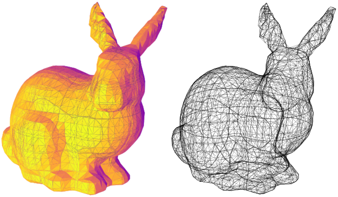
Figure 1: The normal map and skeleton visualization are analytically generated from piecewise trilinear networks, comprising both HashGrid (Müller et al., 2022) and ReLU neural networks, that have been trained to learn a signed distance function with the eikonal loss for the Stanford bunny (Curless & Levoy, 1996).

Focusing on the successful and widely-adopted trilinear interpolating methods, we present novel theoretical insights and a practical methodology for precise mesh extraction. Following a novel review of the edge subdivision method (Berzins, 2023), an efficient mesh extraction technique for CPWA functions, within the framework of tropical geometry (Section 3), we demonstrate that ReLU neural networks incorporating the trilinear module are piecewise trilinear networks (Definition 4.1). Then, we establish that the hypersurface within the trilinear region becomes a plane under the eikonal (Bruns, 1895) constraint (Theorem 4.5), a common practice during the training of SDF.

Building upon this observation, we propose a method for approximating the determination of intersecting points among three hypersurfaces. Given the inherent curvature of these surfaces, achieving an exact solution is infeasible. In our approach, we utilize two hypersurfaces and a diagonal plane for a more feasible and precise approximation (Theorem 4.7). Additionally, we introduce a methodology for arranging vertices composed of faces to implicitly represent normal vectors. We experimentally confirm accuracy and simplicity using chamfer distance, efficiency, and angular distance, simultaneously exploring the relationship between the eikonal loss and the planarity of the hypersurface. In Figure 1, we present the analytically generated normal map and skeleton visualizations produced by our method using piecewise trilinear networks composed of HashGrid and ReLU neural networks. For a more detailed view and comprehensive explanations, please refer to Figure 7 in Appendix.

As we delve into this novel avenue, we not only aim to extend the existing visualization techniques to trilinear neural networks but also to explore potential new directions stemming from the applications of mesh extraction, e.g., baking for real-time rendering or geometric loss using extracted geometry (Berzins, 2023) in future work.

Our contributions are summarized as follows:

1. We present novel theoretical insights and a practical methodology for precise mesh extraction, employing piecewise trilinear networks.

2. This provides a theoretical exposition of the eikonal constraint, revealing that within the trilinear region, the hypersurface transforms into a plane.

3. We empirically validate correctness and parsimony through chamfer distance and efficiency, and angular distance, while examining the correlation between the eikonal loss and hypersurface planarity.

2 Related Work

Mesh extraction in deep neural networks.

A conventional black-box approach is to assess a given function at sampled points to derive the complex of the function, commonly implemented through marching cubes (Lorensen & Cline, 1987) or marching tetrahedra (Doi & Koide, 1991; Shen et al., 2021). Despite the inclusion of mesh optimization techniques (Hoppe et al., 1993) in modern mesh packages, this exhaustive method is still inclined to generate redundant complexities due to the discretization, needlessly burdening the computational load on a learning pipeline. Aiming for exact extraction, initial efforts focused on identifying linear regions (Serra et al., 2018) and employing Analytical Marching (Lei & Jia, 2020) to exactly reconstruct the zero-level isosurface. Contemporary approaches involve region subdivision, wherein the regions of the complex are progressively subdivided from neuron to neuron and layer to layer, allowing for the efficient calculation of the exponentially increasing linear regions (Raghu et al., 2017; Hanin & Rolnick, 2019; Humayun et al., 2023; Berzins, 2023). Nevertheless, many previous studies have explored CPWA functions consisting of fully connected layers and ReLU activation, primarily owing to the mathematical simplicity of hyperplanes defining linear regions. However, this restricts their applications in emerging domains of deep implicit surface learning that diverge from CPWA functions.

Positional encoding.

The spectral bias of a multi-layer perceptron (MLP) hinders to effectively learn high frequencies, both theoretically and empirically (Tancik et al., 2020). To address this limitation, Fourier feature mapping, employing trigonometric projections similar to those used in the Transformer architecture (Vaswani et al., 2017), proves successful in representing complex 3D objects and scenes. Furthermore, to address its slow convergence, positional encoding methods and enhance rendering quality, novel positional encoding methods using trilinear interpolations, e.g., HashGrid (Müller et al., 2022), TensoRF (Chen et al., 2022) are introduced. Both techniques generate positional features through trilinear interpolation among the eight nearest corner features derived from a pre-defined 3D grid. These features are obtained by hashing from multi-resolution hash tables or factorized representations of a feature space, respectively. However, these approaches cause the function represented by neural networks to deviate from CPWA functions, as trilinear interpolation is not an affine transformation. Consequently, this results in the division of complex regions by intricate hypersurfaces.

Eikonal equation and SDF.

An eikonal  equation is a non-linear first-order partial differential equation governing the propagation of wavefronts. Notably, this equation finds application in the regularization of a signed distance function (SDF) in the context of neural surface modeling (Gropp et al., 2020; Wang et al., 2021; Li et al., 2023). If $\Omega$ represents a subset of the space ${\mathcal{X}}$ equipped with the metric $d$, the SDF $f({\bm{x}})$ is defined as follows:

$$f({\bm{x}})=\begin{cases}-d({\bm{x}},\partial\Omega)&\text{if}~{}{\bm{x}}\in\Omega\\ d({\bm{x}},\partial\Omega)&\text{if}~{}{\bm{x}}\in\Omega^{\complement}\\ \end{cases}$$ (1)

where $\partial\Omega$ denotes the boundary of $\Omega$. The metric $d$ is then expressed as:

$$d({\bm{x}},\partial\Omega):=\inf_{{\bm{y}}\in\partial\Omega}d({\bm{x}},{\bm{y}})$$ (2)

where $d$ represents the shortest distance from ${\bm{x}}$ to $\partial\Omega$ in the Euclidean space of ${\mathcal{X}}$. In the context of the Euclidean space with a piecewise smooth boundary, the SDF exhibits differentiability almost everywhere, and its gradient adheres to the eikonal equation. Specifically, for points ${\bm{x}}$ on the boundary, $\nabla f({\bm{x}})=N({\bm{x}})$ where the Jacobian of $f$ represents the outward normal vector, or equivalently, $|\nabla f({\bm{x}})|=1$.

3 Preliminaries

In this section, we present an overview of tropical geometry (Section 3.1) to provide a formal definition of the tropical hypersurface (Section 3.2). This hypersurface is significant as it serves as the decision boundary for ReLU neural networks optimizing an SDF, resulting in the formation of a polyhedral complex. For this, we delve into the examination of the tropical algebra of neural networks (Section 3.3). Furthermore, we discuss the edge subdivision algorithm (Berzins, 2023) for extracting the tropical hypersurface (Section 3.4), and we extend this discussion to include considerations for trilinear interpolation in Section 4. Given that Section 3.1 to 3.3 offer insights into tropical geometry, illustrating how each neuron contributes to forming the polyhedral complex, you may choose to skip these subsections if you are already acquainted with these concepts.

3.1 Tropical Geometry

Tropical  geometry (Itenberg et al., 2009; Maclagan & Sturmfels, 2021) describes polynomials and their geometric characteristics. As a skeletonized version of algebraic geometry, tropical geometry represents piecewise linear meshes using tropical semiring and tropical polynomial.

The tropical semiring is an algebraic structure that extends real numbers and $-\infty$ with the two operations of tropical sum $\oplus$ and tropical product $\odot$. Tropical sum and product are conveniently replaced with $\max(\cdot)$ and $+$, respectively. Notice that $-\infty$ is the tropical sum identity, zero is the tropical product identity, and these satisfy associativity, commutativity, and distributivity. For example, a classical polynomial $x^{3}+2xy+y^{4}$ would represent $\max(3x,~{}x+y+2,~{}4y)$. Roughly speaking, this is the tropicalization of the polynomial, denoted tropical polynomial or simply $f$.

3.2 Tropical Hypersurface

The set of points where a tropical polynomial $f$ is non-differentiable, mainly due to tropical sum, $\max(\cdot)$, is called tropical hypersurface, denoted $V(f)$. Note that $V$ is an analogy to the vanishing set of a polynomial.

Definition 3.1 (Tropical hypersurface).

The tropical hypersurface of a tropical polynomial $f({\bm{x}})=c_{1}{\bm{x}}^{\mathrm{\alpha}_{1}}\oplus\cdots\oplus c_{r}{\bm{x}}^{\mathrm{\alpha}_{r}}$ is defined as:

$$V(f)=\{{\bm{x}}\in\mathbb{R}^{d}:c_{i}{\bm{x}}^{\mathrm{\alpha}_{i}}=c_{j}{\bm{x}}^{\mathrm{\alpha}_{j}}=f({\bm{x}})~{}~{}~{}~{}~{}$$

$$~{}~{}~{}~{}~{}\text{for some}~{}~{}~{}\mathrm{\alpha}_{i}\neq\mathrm{\alpha}_{j}\}$$ (3)

where the tropical monomial $c_{i}{\bm{x}}^{\mathrm{\alpha}_{i}}$ with $d$-variate ${\bm{x}}$ is defined as $c\odot x_{1}^{a_{i,1}}\odot\cdots\odot x_{d}^{a_{i,d}}$ with $d$-variate $\mathrm{\alpha}_{i}=(a_{i,1},\dots,a_{i,d})$. In other words, this is the set of points where $f(x)$ equals two or more monomials in $f$.

3.3 Tropical Algebra of Neural Networks

Definition 3.2 (ReLU neural networks).

Without loss of generality, $L$-layer neural networks with ReLU activation are a composition of functions defined as:

$$\nu^{(L)}=\rho^{(L)}\circ\sigma^{(L-1)}\circ\rho^{(L-1)}\cdots\sigma^{(1)}\circ\rho^{(1)}$$ (4)

where $\sigma({\bm{x}})=\max({\bm{x}},0)$ and $\rho^{(i)}({\bm{x}})={\bm{W}}^{(i)}{\bm{x}}+{\bm{b}}^{(i)}$.

Although the neural networks $\nu$ is generally non-convex, it is known that the difference of two tropical signomials can represent $\nu$ (Zhang et al., 2018). A tropical signomial takes the same form as a tropical polynomial (ref. Definition 3.1), but it additionally allows the exponentials $\mathrm{\alpha}$ to be real values rather than integers. With tropical signomials $F$, $G$, and $H$,

$$\nu^{(l)}({\bm{x}}) =H^{(l)}({\bm{x}})-G^{(l)}({\bm{x}})$$ (5)

$$\sigma^{(l)}\nu^{(l)}({\bm{x}}) =F^{(l)}({\bm{x}})-G^{(l)}({\bm{x}})$$ (6)

where $F^{(l)}$, $G^{(l)}$, and $H^{(l)}$ are as follows:

$$F^{(l)}({\bm{x}}) =\max\big{(}H^{(l)}({\bm{x}}),~{}G^{(l)}({\bm{x}})\big{)}$$ (7)

$$G^{(l)}({\bm{x}}) ={\bm{W}}_{+}^{(l)}G^{(l-1)}({\bm{x}})+{\bm{W}}_{-}^{(l)}F^{(l-1)}({\bm{x}})$$ (8)

$$H^{(l)}({\bm{x}}) ={\bm{W}}_{+}^{(l)}F^{(l-1)}({\bm{x}})+{\bm{W}}_{-}^{(l)}G^{(l-1)}({\bm{x}})+{\bm{b}}^{(l)}$$ (9)

while ${\bm{W}}^{(l)}={\bm{W}}_{+}^{(l)}-{\bm{W}}_{-}^{(l)}$ where ${\bm{W}}_{+}^{(l)}$ and ${\bm{W}}_{-}^{(l)}\in\mathbb{R}^{+}$.

Proposition 3.3.

(Decision boundary of neural networks) The decision boundary for $L$-layer neural networks with ReLU activation $\nu^{(L)}({\bm{x}})=0$ is where two tropical monomials, or two arguments of $\max$, equal (Definition 3.1), recursively, as follows:

$${\mathcal{B}}\subseteq\big{\{}{\bm{x}}:\nu_{j}^{(i)}({\bm{x}})=H_{j}^{(i)}({\bm{x}})-G_{j}^{(i)}({\bm{x}})=0,~{}~{}~{}$$

$$i\in(1,\dots,L),~{}j\in(1,\dots,H)\big{\}}$$ (10)

where the subscription $j$ denotes the $j$-th element, assuming the hidden size of neural networks is $H$, while the $L$-th layer has a single output, for simplicity. Remind that tropical operations satisfy the usual laws of arithmetic for recursive consideration.

This implies that piecewise hyperplanes corresponding to the preactivations $\{\nu_{j}^{(i)}\}$ are the candidates shaping the decision boundary. Each linear region has the same pattern of zero masking by $\textrm{ReLU}(\cdot)$, effectively making it linear as an equation of a plane. In turn, if the pattern changes as an input is continually changed, it moves to another linear region. From a geometric point of view, this is why the number of linear regions grows polynomially with the hidden size $H$ and exponentially with the number of layers $L$ (Zhang et al., 2018; Serra et al., 2018).

3.4 Edge Subdivision for Tropical Geometry

Polyhedral  complex derivation from a multitude of linear regions is inefficient and may be infeasible in some cases. Rather, Berzins (2023) argue that tracking vertices and edges of the decision boundary sequentially considering the polynomial number of hyperplanes is particularly efficient, even enabling parallel tensor computations.

Initially, we start with a unit cube of eight vertices and a dozen edges, denoted by ${\mathcal{V}}$ and ${\mathcal{E}}$, respectively. For each piecewise linear, or folded in their term, hyperplane, we find the intersection points of each one of the edges and the hyperplane (if any) to add to ${\mathcal{V}}$. The divided edges by the intersection are also added to ${\mathcal{E}}$. Note that we find new edges of polygons, the intersections of convex polyhedra representing corresponding linear regions (Grigsby & Lindsey, 2022), and the folded hyperplane. Repeating these for all folded hyperplanes, before selecting all vertices ${\bm{x}}^{\star}$ where $\nu({\bm{x}}^{\star})=0$. Then, the corresponding edges would represent the decision boundary.

To elaborate with details, the order of subdivising is invariant as stated in Proposition 3.3; however, we must perform the subdivision with all hyperplanes in the previous layers in advance if we want to keep the current set of edges not crossing linear regions. One critical advantage of this principle is that we can find the intersection point by evaluating the output ratio of the two vertices of an edge, $\nu({\bm{x}}_{0})$ and $\nu({\bm{x}}_{1})$, which are proportional to the distances to the hyperplane by Thales’s theorem (Friedrich et al., 2008). The intersection point would simply be $\hat{{\bm{x}}}_{0,1}=(1-w){\bm{x}}_{0}+w{\bm{x}}_{1}$ where $w=|d_{0}|/|d_{0}-d_{1}|$ and $d_{k}=\nu_{j}^{(l)}({\bm{x}}_{k})$, upon the fact that $d_{0}\cdot d_{1}<0$ if the hyperplane divides the edge.

Updating edges needs two steps: dividing the edge into two new edges and adding new edges of intersectional polygons by a hyperplane for convex polyhedra representing linear regions. The latter is a tricky part that we need to find every pair of two vertices among $\{\hat{{\bm{x}}}_{\cdot,\cdot}\}$, both within the same linear region and on the two common hyperplanes, obviously including the current hyperplane. They argue that the sign-vectors for the preactivations provide an efficient way to find them.

Definition 3.4 (Sign-vectors).

For the current hyperplane specified by the $i^{*}$-th layer and its $j^{*}$-th preactivation, we define the sign-vectors with a small positive constant $\epsilon$:

$$\gamma({\bm{x}}_{k})_{\phi(i,j)} =\begin{cases}+1&\text{if }~{}\nu^{(i)}_{j}({\bm{x}}_{k})~{}~{}>+\epsilon\\ ~{}~{}~{}0&\text{if }|\nu^{(i)}_{j}({\bm{x}}_{k})|~{}\leq+\epsilon\\ -1&\text{if }~{}\nu^{(i)}_{j}({\bm{x}}_{k})~{}~{}<-\epsilon\end{cases}$$ (11)

for all $i$ and $j$ where $\phi(i,j)\leq\phi(i^{*},j^{*})$, and $\phi(i,j)$ is an ascending indexing function from lower layers, to vectorize a signed matrix, handling arbitrary hidden sizes of networks.

Notice that a hyperplane divides a space into two half-spaces, two linear regions. Collectively, if the sign-vectors for the $i$-th layer and its $j$-th preactivation of two vertices have the same values except for zeros, which are wild cards for matching, we can say that the two vertices are within the same linear region in the current step $(i^{*},j^{*})$. For the second, the sign-vector has at least three zeros specifying a point by at least three hyperplanes. If two zeros are at the same indices in the two sign-vectors, the two vertices are on the same two hyperplanes, forming an edge. Notice that our principle asserts edges should be within linear regions.

They argue that the edge subdivision provides the optimal time and memory complexities of ${\mathcal{O}}(|{\mathcal{V}}|)$, linear in the number of vertices, while it can be efficiently computed in parallel. According to Hanin & Rolnick (2019), the number of linear regions is known for $o(N^{L}/L!)$ where $N$ is the total number of neurons, or $\phi(L,1)$ in our notation.

4 Method

4.1 Piecewise Trilinear Networks

Definition 4.1 (Trilinear interpolation).

Let a unit hypercube be in the $D$-dimensional space, where its $2^{D}$ corners are represented by ${\bm{H}}\in\mathbb{R}^{2^{D}\times F}$. Given a weight ${\bm{w}}\in[0,1]^{D}$, the interpolation $\psi$ is defined as:

$$\psi({\bm{w}};{\bm{H}})=\sum_{i=0}^{2^{D}-1}\omega(i,{\bm{w}})\cdot{\bm{H}}_{i}~{}~{}~{}\in\mathbb{R}^{F}$$ (12)

where the interpolating weight $\omega(i,{\bm{w}})\in\mathbb{R}$ is defined using a left-aligned and zero-trailing binarization function $\textrm{B}\in\{0,1\}^{D}$ as follows:

$$\omega(i,{\bm{w}})=\prod_{j=1}^{D}(1-\textrm{B}(i)_{j})(1-{\bm{w}}_{j})+\textrm{B}(i)_{j}{\bm{w}}_{j}$$ (13)

which is the volume of the opposite subsection of the hypercube divided by the weight point ${\bm{w}}$. For a general hypercube, scaling the weight for a unit hypercube gets the same result. Trilinear interpolation extends linear and bilinear interpolations to three dimensions, where $D=3$.

Lemma 4.2 (Nested trilinear interpolation).

Let a nested cube be inside of a unit cube, where its positions of the eight corners deviate $-{\bm{a}}_{j}$ or $+{\bm{b}}_{j}$, such that ${\bm{a}}_{j},{\bm{b}}_{j}\geq 0$, from ${\bm{w}}_{j}$ for each dimension $j$, using the notations of Definition 4.1. The eight corners of the nested cube are the trilinear interpolations of the eight corners of the unit cube. Then, the trilinear interpolation with the unit cube and the nested cube for ${\bm{w}}$ is identical.

Proof.

Notice that trilinear interpolation is linear for each dimension to prove it. The detailed proof can be found in Lemma A.1. ∎

Definition 4.3 (Piecewise trilinear networks).

Let a positional encoding module be $\tau:\mathbb{R}^{D}\rightarrow\mathbb{R}^{F}$ using the trilinear interpolation of spatially nearby learnable vectors on a three-dimensional grid, e.g., HashGrid (Müller et al., 2022) or TensoRF (Chen et al., 2022). Usually, they transform the input coordinate ${\bm{x}}$ to ${\bm{w}}$ with a multi-resolution scale and find a relative position within a grid cell. Then, we define trilinear neural networks $\tilde{\nu}$, by prepending $\tau$ to the neural networks $\nu$ from Definition 3.2. The input and output dimensions of $\nu$ are adapted to $F$ and $1$, respectively.

$$\tilde{\nu}^{(L)}=\nu^{(L)}\circ\tau$$ (14)

Note that $\tau$ is grid-wise trilinear. Using Lemma 4.2, $\tilde{\nu}$ is trilinear within the composite intersections of linear regions of $\nu$ and trilinear regions of $\tau$ if available. (We will discuss how to access the cubic corner features in the case that trilinear regions are no longer cubic in Section 5.3.) Then, we regard $\tilde{\nu}$ as piecewise trilinear.

4.2 Curved Edge Subdivision in a Trilinear Space

In a trilinear space, $\tau$ projects a line to a curve except the lines on the grid. Notably, the diagonal line ${\bm{t}}=(t,t,t)^{\intercal}$ where $t\in[0,1]$ is projected to a cubic Bézier curve (ref. Proposition A.2). We aim to generalize for the curved edge subdivision for hypersurfaces.

Lemma 4.4 (Curved edge of two hypersurfaces).

In a piecewise trilinear region, let an edge $({\bm{x}}_{0},{\bm{x}}_{7})$ be the intersection of two hypersurfaces $\tilde{\nu}_{i}({\bm{x}})=\tilde{\nu}_{j}({\bm{x}})=0$, while ${\bm{x}}_{0}$ and ${\bm{x}}_{7}$ are on the two hypersurfaces. Then, the edge is defined as:

$$\{{\bm{x}}:\tau({\bm{x}})=(1-t)\tau({\bm{x}}_{0})+t\tau({\bm{x}}_{7})\hskip 40.00006pt$$

$$~{}~{}\text{where}~{}~{}{\bm{x}}\in\mathbb{R}^{D}~{}~{}\text{and}~{}~{}t\in\mathbb{R}\}.$$ (15)

Proof.

The detailed proof is provided in Lemma A.4. ∎

Notice that it does not decrease the number of variables to find a line solution since the trilinear interpolation $\tau$ forms hypersurfaces making complex cases. Yet, we theoretically demonstrate that the eikonal constraints on $\tilde{\nu}$ render them hyperplanes with linear solutions.

Theorem 4.5 (Hypersurface and eikonal constraint).

A hypersurface $\tau({\bm{x}})=0$ passing two points $\tau({\bm{x}}_{0})=\tau({\bm{x}}_{7})=0$ while $\tau({\bm{x}}_{1\dots 6})\neq 0$ satisfies the eikonal constraint $\|\nabla\tau({\bm{x}})\|_{2}=1$ for all ${\bm{x}}\in[0,1]^{3}$. Then, the hypersurface of $\tau({\bm{x}})=0$ is a plane.

Corollary 4.6 (Affine-transformed hypersurface and eikonal constraint).

Let $\nu_{0}({\bm{x}})$ and $\nu_{1}({\bm{x}})$ be two affine transformations defined by ${\bm{W}}_{i}^{\intercal}{\bm{x}}+{\bm{b}}_{i}$, $i\in\{0,1\}$. A hypersurface $\nu_{0}\big{(}\tau({\bm{x}})\big{)}=0$ passing two points $\nu_{0}\big{(}\tau({\bm{x}}_{0})\big{)}=\nu_{0}\big{(}\tau({\bm{x}}_{7})\big{)}=0$ while $\nu_{0}\big{(}\tau({\bm{x}}_{1\dots 6})\big{)}\neq 0$ satisfies the eikonal constraint $\|\nabla\nu_{1}\big{(}\tau({\bm{x}})\big{)}\|_{2}=1$ for all ${\bm{x}}\in[0,1]^{3}$. Then, the hypersurface of $\nu_{0}\big{(}\tau({\bm{x}})\big{)}=0$ is a plane.

The proofs can be found in Theorem A.5 and Corollary A.6

Since we aim for a polyhedral complex derivation that piecewise trilinear networks represent, we replace one of the hypersurfaces (possibly) forming the curved edge with a diagonal plane in a piecewise trilinear region. We opt for this choice not only due to its mathematical simplicity but also the characteristics of trilinear hypersurfaces as illustrated in Figure 6, Appendix. Thus, the new vertices lie on at least two hypersurfaces, and the new edges exist on the same hypersurface, while the eikonal constraint minimizes any associated error. This error is tolerated by the hyperparameter $\epsilon$ as specified in Definition 3.4.

Theorem 4.7 (Intersection of two hypersurfaces and a diagonal plane).

Let $\tilde{\nu}_{0}({\bm{x}})=0$ and $\tilde{\nu}_{1}({\bm{x}})=0$ be two hypersurfaces passing two points ${\bm{x}}_{0}$ and ${\bm{x}}_{7}$ such that $\tilde{\nu}_{0}({\bm{x}}_{0})=\tilde{\nu}_{1}({\bm{x}}_{0})=0$ and $\tilde{\nu}_{0}({\bm{x}}_{7})=\tilde{\nu}_{1}({\bm{x}}_{7})=0$, ${\bm{P}}_{i}:=\tilde{\nu}_{0}({\bm{x}}_{i})$ and ${\bm{Q}}_{i}:=\tilde{\nu}_{1}({\bm{x}}_{i})$, ${\bm{P}}_{\alpha}=\big{[}{\bm{P}}_{0};~{}{\bm{P}}_{1};~{}{\bm{P}}_{4};~{}{\bm{P}}_{5}\big{]}$, ${\bm{P}}_{\beta}=\big{[}{\bm{P}}_{2};~{}{\bm{P}}_{3};~{}{\bm{P}}_{6};~{}{\bm{P}}_{7}\big{]}$, and ${\bm{X}}=[(1-x)^{2};~{}x(1-x);~{}(1-x)x;~{}x^{2}]$. Then, $x,z\in[0,1]$ of the intersection point of the two hypersurfaces and a diagonal plane of $x=z$ is the solution of the following quartic equation:

$${\bm{X}}^{\intercal}\big{(}{\bm{P}}_{\alpha}{\bm{Q}}_{\beta}^{\intercal}-{\bm{P}}_{\beta}{\bm{Q}}_{\alpha}^{\intercal}\big{)}{\bm{X}}=0$$ (16)

while

$$y =\frac{{\bm{X}}^{\intercal}{\bm{P}}_{\alpha}}{{\bm{X}}^{\intercal}({\bm{P}}_{\alpha}-{\bm{P}}_{\beta})}\hskip 20.00003pt({\bm{P}}_{\alpha}\neq{\bm{P}}_{\beta}).$$ (17)

Proof.

Please refer to Theorem A.7 for the proof. ∎

Note that finding roots of a polynomial is the eigenvalue decomposition of a companion matrix (Edelman & Murakami, 1995), which can be parallelized (ref. Lemma A.8). Given that the companion matrix remains small for a quartic equation in $\mathbb{R}^{4\times 4}$, the overall complexity remains $\mathcal{O}(|\mathcal{V}|)$. For the detailed complexity analysis on the proposed method, please refer to Appendix B.

4.3 Skeletonization

Skeletonization selects the vertices such that:

$${\mathcal{V}}^{\star}=\{{\bm{x}}|\tilde{\nu}({\bm{x}})\leq\epsilon,{\bm{x}}\in{\mathcal{V}}\}$$ (18)

and the edges ${\mathcal{E}}^{\star}$ such that their two vertices are among ${\mathcal{V}}^{\star}$.

4.4 Faces and Normals

Edges lying on the same plane and a shared region form a face, and this alignment can be determined by evaluating the sign-vectors (ref. Definition 3.4 and Section 5.2). It is important to note that faces are not inherently triangular; however, if needed, they can be triangulated via triangularization for further analysis. The order of vertices conventionally describes its normal. Let ${\bm{x}}_{0}$, ${\bm{x}}_{1}$, and ${\bm{x}}_{2}$ be the vertices forming a triangular face. The normal is defined as follows:

$${\bm{n}}=({\bm{x}}_{1}-{\bm{x}}_{0})\times({\bm{x}}_{2}-{\bm{x}}_{0})$$ (19)

where $\times$ denotes cross product, and the normal is orthogonal to both vectors, with a direction given by the right-hand rule. If the viewing direction aligns opposite to the normal, the order of vertices follows a counter-clockwise arrangement.

We determine the vertex order based on the normal derived from the Jacobian of the mean of vertices. Using cosine similarity to compute relative angles $\theta\in[-\pi,\pi]$ and cross product for getting direction, we identify the counter-clockwise arrangement of vertices, as outlined in Algorithm 1.

Algorithm 1 Sorting Polygon Vertices

  Input: vertices ${\bm{x}}_{i}$, normal ${\bm{n}}$, $N=|\{{\bm{x}}_{i}\}|$

  $\mu=\sum_{i}{\bm{x}}_{i}/N$

  for $i=0$ to $N-1$ do

     ${\bm{v}}_{i}=({\bm{x}}_{i}-\mu)/\|{\bm{x}}_{i}-\mu\|_{2}$

     ${\bm{c}}_{i}=\langle{\bm{v}}_{i},~{}{\bm{v}}_{0}\rangle$,   ${\bm{d}}_{i}=\langle{\bm{v}}_{i}\times{\bm{v}}_{0},~{}{\bm{n}}\rangle$

     $\theta_{i}={\bm{c}}_{i}(2\cdot{\bm{1}}_{{\bm{d}}_{i}\geq 0}-1)+2\cdot{\bm{1}}_{{\bm{d}}_{i}<0}$

  end for

  return $\text{ArgSort}(\{-\theta_{i}\})$

5 Implementation

We employ the HashGrid (Müller et al., 2022) for $\tau$, although any encoding using trilinear interpolation we defined can be applied. We illustrate our method in Algorithm 3 and 4, describing the details in the following sections.

5.1 Initialization

While the edge subdivision (Berzins, 2023) starts with a unit cube of eight vertices and a dozen edges, we know that the unit cube is subdivided by orthogonal planes consisting of the grid. Let an input coordinate be ${\bm{x}}\in[0,1]^{3}$, and there is a unit cube such that one of its corners is at the origin. Taking into account multi-resolution grids, we obtain the marks $m_{i}$, such that the grid planes are $x=m_{i}$, $y=m_{i}$, and $z=m_{i}$, following Algorithm 2. Notice that we carefully consider the offset $s/2$, which prevents the zero derivatives from aligning across all resolution levels (ref. Appendix A of Müller et al. (2022)). Leveraging the obtained marks, we derive the associated grid vertices and edges, which serve as the initial sets for ${\mathcal{V}}$ and ${\mathcal{E}}$, respectively.

Algorithm 2 HashGrid Marks

  Input: Resolution levels $L$, base resolution $N_{\text{min}}$, max resolution $N_{\text{max}}$

  $m=\{0,~{}1\}$

  $b=\log_{2}(N_{\text{max}}/N_{\text{min}})/(L-1)$

  for $l=0$ to $L-1$ do

     $s=1/\big{(}N_{\text{min}}\cdot\exp_{2}(l\cdot b)-1\big{)}$

     $m\leftarrow m+\text{Max}\big{(}\text{Arange}(-s/2,~{}1,~{}s),~{}0\big{)}$

  end for

  return $\text{Sort}\big{(}\text{Unique}(m)\big{)}$

5.2 Optimizing Sign-vectors

The number of orthogonal planes may significantly surpass the number of neurons, making it impractical to allocate elements for the sign-vectors (Definition 3.4). To address this, leveraging the orthogonality of the grid planes, we store a plane index along with an indicator of whether the input is on the plane ($\gamma=0$) or not ($\gamma=1$), similarly.

5.3 Piecewise Trilinear Region

In Theorem 4.7, we need the outputs of corners ${\bm{P}}$ and ${\bm{Q}}$ in a common piecewise trilinear region; however, some corners may be outside of the region. For this, we replace all ReLU activations using the mask ${\bm{m}}$ that:

$${\bm{m}}_{j}^{(i)}=(\tilde{\nu}_{j}^{(i)}({\bm{x}}_{0})>\epsilon)~{}|~{}(\tilde{\nu}_{j}^{(i)}({\bm{x}}_{7})>\epsilon),$$ (20)

where ${\bm{x}}_{0}$ and ${\bm{x}}_{7}$ are the vertices of an edge of interest, for the calculated cubic corners ${\bm{x}}_{0\dots 7}$. This implies that $\nu$ exhibits linearity, except for instances where two vertices simultaneously deviate from linearity. Moreover, as explained in Section 5.1, we can ensure that each edge resides within a shared trilinear region.

For ${\bm{P}}$ and ${\bm{Q}}$, we select the last two pairs of $i$ and $j$ such that $\gamma_{\phi(i,j)}({\bm{x}}_{0})=\gamma_{\phi(i,j)}({\bm{x}}_{7})=0$, indicating two common hypersurfaces passing two points ${\bm{x}}_{0}$ and ${\bm{x}}_{7}$.

Algorithm 3 Polyhedral Complex Derivation

  Input: Sets of vertices ${\mathcal{V}}$ and edges ${\mathcal{E}}$ (from Section 5.1), # of layer $L$, hidden size $H$, trilinear networks $\tilde{\nu}$

  for $i=0$ to $L-1$ do

     for $j=0$ to $H-1$ do

        ${\mathcal{V}},{\mathcal{E}}=$ CurvedEdgeSubdivision$({\mathcal{V}},{\mathcal{E}},\tilde{\nu},i,j)$

     end for

  end for

  ${\mathcal{V}},{\mathcal{E}}=$ CurvedEdgeSubdivision$({\mathcal{V}},{\mathcal{E}},\tilde{\nu},L,0)$

  ${\mathcal{V}}^{\star},{\mathcal{E}}^{\star}=$ Skeletonize$({\mathcal{V}},{\mathcal{E}},\tilde{\nu},\epsilon)$ $\triangleright$ Section 4.3

  ${\mathcal{F}}^{\star}=$ ExtractFaces$({\mathcal{V}}^{\star},{\mathcal{E}}^{\star})$ $\triangleright$ Section 4.4

  return ${\mathcal{V}}^{\star},{\mathcal{E}}^{\star},{\mathcal{F}}^{\star}$

Algorithm 4 Curved Edge Subdivision

  Input: A set of vertices ${\mathcal{V}}$, a set of edges ${\mathcal{E}}$, trilinear networks $\tilde{\nu}$, layer index $i$, neuron index $j$

  $d=\tilde{\nu}({\mathcal{V}};i,j)$

  ${\mathcal{V}}_{\text{new}}=\emptyset$

  for $e$ in ${\mathcal{E}}$ do

     if $d_{e_{0}}\cdot d_{e_{1}}<0$ then

        ${\bm{P}},{\bm{Q}}=$ Corners$(e)$ $\triangleright$ Section 5.3

        ${\bm{x}}_{\text{new}}=$ Intersect$({\bm{P}},{\bm{Q}},e)$ $\triangleright$ Theorem 4.7

        ${\mathcal{V}}_{\text{new}}\leftarrow{\mathcal{V}}_{\text{new}}+\{{\bm{x}}_{\text{new}}\}$

        $e\leftarrow[e_{0},~{}\text{Index}({\bm{x}}_{\text{new}})]$

        ${\mathcal{E}}\leftarrow{\mathcal{E}}+\{[e_{1},~{}\text{Index}({\bm{x}}_{\text{new}})]\}$

     end if

  end for

  ${\mathcal{V}}\leftarrow{\mathcal{V}}+{\mathcal{V}}_{\text{new}}$

  ${\mathcal{E}}\leftarrow{\mathcal{E}}+$ FindPolygons$({\mathcal{V}}_{\text{new}})$ $\triangleright$ Section 3.4

  return ${\mathcal{V}}$, ${\mathcal{E}}$

6 Experiments

6.1 Hyperparameter

For ReLU neural networks, the number of layers $L$ of 3, hidden size $H$ of 16, and $\epsilon$ of 1e-4 for the sign-vectors (ref. Definition 3.4). The weight for the eikonal loss is 1e-2. For HashGrid, the resolution levels of 4, feature size of 2, base resolution $N_{\text{min}}$ of 2, and max resolution $N_{\text{max}}$ of 16 (sphere) or 32 (bunny). We use the official Python package of tinycudnn  for the HashGrid module.

6.2 Chamfer Distance

The chamfer distance is a metric used to evaluate the similarity between two sets of sampled points from two meshes. Let ${\mathcal{S}}_{0}$ and ${\mathcal{S}}_{1}$ be the two sets of points. Specifically, the bidirectional chamfer distance (CD) is defined as follows:

$$\text{CD}({\mathcal{S}}_{0},{\mathcal{S}}_{1}) =\frac{1}{2}\Big{(}\overrightarrow{\text{CD}}({\mathcal{S}}_{0},{\mathcal{S}}_{1})+\overrightarrow{\text{CD}}({\mathcal{S}}_{1},{\mathcal{S}}_{0})\Big{)},$$ (21)

$$\overrightarrow{\text{CD}}({\mathcal{S}}_{0},{\mathcal{S}}_{1}) =\frac{1}{|{\mathcal{S}}_{0}|}\sum_{{\bm{x}}\in{\mathcal{S}}_{0}}\min_{{\bm{y}}\in{\mathcal{S}}_{1}}\|{\bm{x}}-{\bm{y}}\|_{2}^{2}.$$ (22)

We randomly select 100K points on the faces through ray-marching from the origin, directing toward a randomly chosen point on a unit sphere. Additionally, we generate another 100K points by ray-marching from a randomly selected point on the sphere toward the origin, specifically for a non-convex complex. We obtain ${\mathcal{S}}_{1}$ by using marching cubes (MC) with 256³ grid samples as the reference ground truth.

Figure 4 and Figure 4 show the chamfer distances for a unit sphere and the Standford bunny (Curless & Levoy, 1996). Varying the number of samples in marching cubes (Lorensen & Cline, 1987), we plot the baseline with respect to the number of generated vertices. Given that our method, Tropical, extracts vertices from the intersection points of hypersurfaces, we represent the results with a red diagonal cross.

Our approach yields nearly optimal outcomes while being parsimonious in the utilization of vertices for both scenarios. To illustrate, consider the MC achieving a comparable chamfer distance with approximately seven times more vertices and redundancy in surface representation. Specifically, the chamfer efficiency, defined as $1/\big{(}\sqrt{|{\mathcal{V}}|}\times\text{CD}\big{)}$, emphasizes this observation, revealing a ratio of 5.75 (ours) versus 4.68 (MC) as shown in Table 1.

In cases where the target surfaces exhibit planary characteristics, our method inherently holds an advantage over MC in capturing optimal vertices and faces. Nevertheless, when dealing with curved surfaces, our method may not reach the approximation achieved by MC with excessive sampling. A potential approach for our method involves breaking the curved edges to better conform to the learned surfaces. This entails allocating more vertices strategically, aiming for an improved approximation.

Table 1: Chamfer distance (CD) and chamfer efficiency (CE) for the Stanford bunny. The chamfer distance ($\times$1e-7) is evaluated using the marching cubes (MC) with 256³ grid samples as the reference ground truth for all measurements. The chamfer efficiency is succinctly expressed as $1/(\sqrt{|{\mathcal{V}}|}\times\text{CD})$, providing a concise representation of the trade-off between the number of vertices and the chamfer distance. The results are averaged over three random seeds. Please refer to Table 2 in Appendix for standard deviation.

	Sample	$|{\mathcal{V}}|$ $\downarrow$	CD $\downarrow$	CE $\uparrow$	Time $\downarrow$
MC	16	303	1364	4.21	0.00
	24	704	858	4.39	0.00
	32	1338	584	4.68	0.00
	40	2105	513	4.25	0.01
	48	3065	440	4.11	0.04
	56	4202	390	3.96	0.01
	64	5570	325	4.12	0.02
	128	22612	305	2.18	0.10
	196	51343	147	3.00	0.34
	224	70007	161	2.34	0.62
Ours	-	4491	259	5.75	5.66

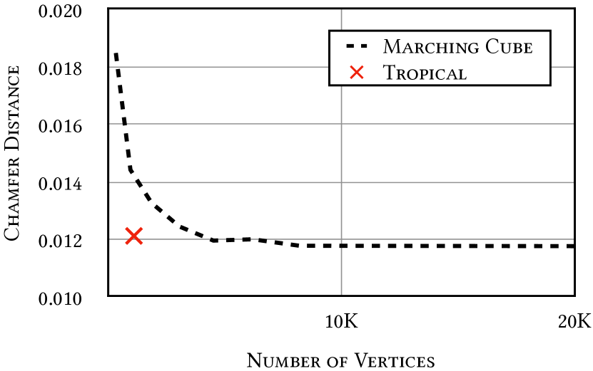
Figure 2: Chamfer distances for a unit sphere varying the number of vertices.

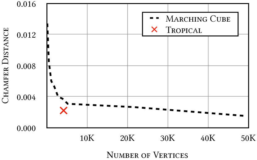
Figure 3: Chamfer distances for the Stanford bunny varying the number of vertices.

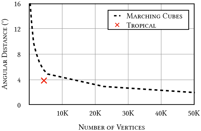
Figure 4: Angular distances of the normal vectors for the Stanford bunny.

Figure 5: Effect of varying the weight of the eikonal loss on the flatness error $\Delta_{\text{flat}}$, as illustrated in Equation 24. For the plot, we conduct experiments using the unit sphere.

6.3 Angular Distance

The angular distance measures how much the normal vectors deviate from the ground truths. Analogous to the chamfer distance, we sample 200K points on the surface and calculate the normal vectors using Equation 19 in Section 4.4. The angular distance is defined as follows:

$$\text{AD}({\mathcal{N}}_{0},{\mathcal{N}}_{1})=\mathbb{E}_{i}\Big{[}\frac{180}{\pi}\cdot\cos^{-1}\big{(}\langle{\mathcal{N}}_{0}^{(i)},{\mathcal{N}}_{1}^{(i)}\rangle\big{)}\Big{]}$$ (23)

In Figure 4, the angular distances of the normal vectors for the Stanford bunny are plotted. As we expected, our approach efficiently estimates the faces using a parsimonious number of vertices compared to the sampling-based method.

6.4 Eikonal Constraint for Planarity

To assess the practical efficacy of the eikonal constraint, which enforces the planarity of hypersurfaces as outlined in Theorem 4.5, we quantify the error associated with the trilinear flat constraints presented in the proof of Theorem A.5 in Appendix. Let ${\bm{x}}_{0}$ and ${\bm{x}}_{7}$ be two vertices consisting of an edge, while ${\bm{x}}_{1\dots 6}$ are its cubic corners. We obtain $\tilde{\nu}({\bm{x}}_{1\dots 6})$ in a piecewise trilinear region as described in Section 5.3. This evaluation is conducted as follows:

$$\Delta_{\text{flat}}= \mathbb{E}_{\mathcal{E}}\Big{[}\frac{1}{2}\big{(}\|\Sigma_{i\in\{1,2,4\}}\tilde{\nu}({\bm{x}}_{i})\|_{1}+\|\Sigma_{i\in\{3,5,6\}}\tilde{\nu}({\bm{x}}_{i})\|_{1}\big{)}$$

$$~{}~{}+\frac{1}{3}\Big{(}\sum_{i=1}^{3}\|\Sigma_{j\in\{i,7-i\}}\tilde{\nu}({\bm{x}}_{j})\|_{1}\Big{)}\Big{]}/2.$$ (24)

In Figure 5, we empirically validate that the eikonal loss enforces planarity in the hypersurfaces within piecewise trilinear regions, as described in Theorem 4.5. Absence of the eikonal loss results in elevated planarity errors, leading to the construction of an inaccurate mesh.

7 Limitation

In Section 4.4, the extraction of faces, including getting normal vectors and vertex sorting, gathers vertices on the same plane within a trilinear region for our visualization. To achieve this, we initially implemented a naive approach by creating a dictionary mapping regions to vertices through the iteration over the identified regions. However, we acknowledge the potential for further optimization to enhance efficiency. The process currently takes $3.23\pm 0.06$ seconds, constituting approximately 79% of the total time spent, excluding the plotting phase. Notice that we provided the detailed complexity analysis on our method in Appendix B.

8 Conclusions

In conclusion, our exploration of novel techniques in visualizing trilinear neural networks unveils intricate structures and extends mesh extraction applications beyond CPWA functions. Focused on trilinear interpolating methods, our study yields novel theoretical insights and a practical methodology for precise mesh extraction. Notably, Theorem 4.5 shows the transformation of hypersurfaces to planes within the trilinear region under the eikonal constraint. Empirical validation using chamfer distance and efficiency, and angular distance affirms the correctness and parsimony of our methodology. The correlation analysis between eikonal loss and hypersurface planarity adds depth to our understanding. Our proposed method for approximating intersecting points among three hypersurfaces, coupled with a vertex arrangement methodology, broadens the applications of our techniques. This work establishes a foundation for future research and practical applications in the evolving landscape of deep neural network analysis and real-time rendering mesh extraction.

Broader Impact and Ethical Considerations

This work aims to advance machine learning through improved mesh extraction techniques from neural surface representations. Ethical aspects align with established norms in the field, focusing on theoretical insights, analytical methods, and empirical validations for broader applications.

Appendix A Theoretical Proofs

Lemma A.1.

(Nested trilinear interpolation, restated) Let a nested cube be inside of a unit cube, where its positions of the eight corners deviate $-{\bm{a}}_{j}$ or $+{\bm{b}}_{j}$, such that ${\bm{a}}_{j},{\bm{b}}_{j}\geq 0$, from ${\bm{w}}_{j}$ for each dimension $j$, using the notations of Definition 4.1. The eight corners of the nested cube are the trilinear interpolations of the eight corners of the unit cube. Then, the trilinear interpolation with the unit cube and the nested cube for ${\bm{w}}$ is identical.

Proof.

Let a left-aligned and zero-trailing binarization function be $\textrm{B}(\cdot)\in\{0,1\}^{D}$ and $D=3$. The partial derivative of the trilinear interpolation with the nested cube $\hat{{\bm{H}}}$ with respect to ${\bm{H}}_{7}$ and ${\bm{H}}_{0}$ would be:

$$\frac{\partial\phi({\bm{w}};\hat{{\bm{H}}})}{\partial{\bm{H}}_{7}} =\sum_{i=0}^{2^{D}-1}\prod_{j=1}^{D}\frac{(1-\textrm{B}(i)_{j}){\bm{b}}_{j}({\bm{w}}_{j}-{\bm{a}}_{j})+\textrm{B}(i)_{j}{\bm{a}}_{j}({\bm{w}}_{j}+{\bm{b}}_{j})}{{\bm{a}}_{j}+{\bm{b}}_{j}}$$ (25)

$$=\sum_{i=0}^{2^{D-1}-1}\frac{{\bm{b}}_{D}({\bm{w}}_{D}-{\bm{a}}_{D})+{\bm{a}}_{D}({\bm{w}}_{D}+{\bm{b}}_{D})}{{\bm{a}}_{D}+{\bm{b}}_{D}}\prod_{j=1}^{D-1}\frac{(1-\textrm{B}(i)_{j}){\bm{b}}_{j}({\bm{w}}_{j}-{\bm{a}}_{j})+\textrm{B}(i)_{j}{\bm{a}}_{j}({\bm{w}}_{j}+{\bm{b}}_{j})}{{\bm{a}}_{j}+{\bm{b}}_{j}}$$ (26)

$$={\bm{w}}_{D}\sum_{i=0}^{2^{D-1}-1}\prod_{j=1}^{D-1}\frac{(1-\textrm{B}(i)_{j}){\bm{b}}_{j}({\bm{w}}_{j}-{\bm{a}}_{j})+\textrm{B}(i)_{j}{\bm{a}}_{j}({\bm{w}}_{j}+{\bm{b}}_{j})}{{\bm{a}}_{j}+{\bm{b}}_{j}}$$ (27)

$$=\prod_{j=1}^{D}{\bm{w}}_{j}=\frac{\partial\phi({\bm{w}};{\bm{H}})}{\partial{\bm{H}}_{7}}$$ (28)

and

$$\frac{\partial\phi({\bm{w}};\hat{{\bm{H}}})}{\partial{\bm{H}}_{0}} =\sum_{i=0}^{2^{D}-1}\prod_{j=1}^{D}\frac{(1-\textrm{B}(i)_{j}){\bm{b}}_{j}(1-{\bm{w}}_{j}+{\bm{a}}_{j})+\textrm{B}(i)_{j}{\bm{a}}_{j}(1-{\bm{w}}_{j}-{\bm{b}}_{j})}{{\bm{a}}_{j}+{\bm{b}}_{j}}$$ (29)

$$=(1-{\bm{w}}_{D})\sum_{i=0}^{2^{D-1}-1}\prod_{j=1}^{D-1}\frac{(1-\textrm{B}(i)_{j}){\bm{b}}_{j}(1-{\bm{w}}_{j}+{\bm{a}}_{j})+\textrm{B}(i)_{j}{\bm{a}}_{j}(1-{\bm{w}}_{j}-{\bm{b}}_{j})}{{\bm{a}}_{j}+{\bm{b}}_{j}}$$ (30)

$$=\prod_{j=1}^{D}(1-{\bm{w}}_{j})=\frac{\partial\phi({\bm{w}};{\bm{H}})}{\partial{\bm{H}}_{0}},$$ (31)

respectively. In a similar way, we can describe the other cases ${\bm{H}}_{1}$ to ${\bm{H}}_{6}$ of the nested trilinear weights since there are two cases for each dimension inside the product. ∎

Proposition A.2 (Cubic Bézier curve).

Trilinear interpolation from Definition 4.1 with the weights on the diagonal line ${\bm{t}}=(t,t,t)^{\intercal}$ where $t\in[0,1]$ is a cubic Bézier curve.

Proof.

We rewrite the trilinear interpolation from Definition 4.1 with the weight ${\bm{t}}$ as follows:

$$\psi({\bm{t}};{\bm{H}}) =\sum_{i=0}^{2^{3}-1}\omega(i,{\bm{t}})\cdot{\bm{H}}_{i}$$ (32)

$$=\sum_{i=0}^{2^{3}-1}\prod_{j=1}^{3}\Big{[}(1-\textrm{B}(i)_{j})(1-t)+\textrm{B}(i)_{j}t\Big{]}\cdot{\bm{H}}_{i}$$ (33)

$$=(1-t)^{3}{\bm{H}}_{0}+(1-t)^{2}t({\bm{H}}_{1}+{\bm{H}}_{2}+{\bm{H}}_{4})+(1-t)t^{2}({\bm{H}}_{3}+{\bm{H}}_{5}+{\bm{H}}_{6})+t^{3}{\bm{H}}_{7}$$ (34)

$$=(1-t)^{3}{\bm{H}}_{0}+3(1-t)^{2}t(\frac{{\bm{H}}_{1}+{\bm{H}}_{2}+{\bm{H}}_{4}}{3})+3(1-t)t^{2}(\frac{{\bm{H}}_{3}+{\bm{H}}_{5}+{\bm{H}}_{6}}{3})+t^{3}{\bm{H}}_{7}$$ (35)

$$=(1-t)^{3}{\bm{P}}_{0}+3(1-t)^{2}t{\bm{P}}_{1}+3(1-t)t^{2}{\bm{P}}_{2}+t^{3}{\bm{P}}_{3}$$ (36)

Four points ${\bm{P}}_{0}:={\bm{H}}_{0}$, ${\bm{P}}_{1}:=\frac{{\bm{H}}_{1}+{\bm{H}}_{2}+{\bm{H}}_{4}}{3}$, ${\bm{P}}_{2}:=\frac{{\bm{H}}_{3}+{\bm{H}}_{5}+{\bm{H}}_{6}}{3}$, and ${\bm{P}}_{3}:={\bm{H}}_{7}$ define the cubic Bézier curve. ∎

As $t$ is changed from zero to one, the curve starts at ${\bm{P}}_{0}$ going toward ${\bm{P}}_{1}$ and turns in the direction of ${\bm{P}}_{2}$ before arriving at ${\bm{P}}_{3}$. Usually, the curve does not pass ${\bm{P}}_{1}$ nor ${\bm{P}}_{2}$; but these give the directional guide for the curve.

Lemma A.3 (Hypersurfaces in a trilinear space).

In a piecewise trilinear region where ${\bm{x}}$ lies, hypersurfaces of the piecewise trilinear networks are defined as follows, following the notation of Definition 4.1:

$$0=\tilde{\nu}({\bm{x}}) =\sum_{i=0}^{2^{D}-1}\omega(i,{\bm{w}})\cdot\tilde{\nu}({\bm{x}}_{i})$$ (37)

where ${\bm{w}}\in[0,1]^{D}$ is the relative position in a grid cell and $\{{\bm{x}}_{i}\}$ and $\{{\bm{H}}_{i}\}$ are the corresponding corner positions and representations, respectively, in a trilinear space.

Proof.

In a piecewise trilinear region, we can use the linearity of $\nu$ as follows:

$$\tilde{\nu}({\bm{x}}) =\big{(}\nu\circ\tau\big{)}({\bm{x}})$$ (38)

$$=\nu\Big{(}\sum_{i=0}^{2^{D}-1}\omega(i,{\bm{w}})\cdot{\bm{H}}_{i}\Big{)}$$ (39)

$$=\sum_{i=0}^{2^{D}-1}\omega(i,{\bm{w}})\cdot\nu\big{(}{\bm{H}}_{i}\big{)}$$ (40)

$$=\sum_{i=0}^{2^{D}-1}\omega(i,{\bm{w}})\cdot\tilde{\nu}\big{(}{\bm{x}}_{i}\big{)}$$ (41)

which concludes the proof. ∎

Lemma A.4 (Curved edge of two hypersurfaces, restated).

In a piecewise trilinear region, let an edge $({\bm{x}}_{0},{\bm{x}}_{7})$ be the intersection of two hypersurfaces $\tilde{\nu}_{i}({\bm{x}})=\tilde{\nu}_{j}({\bm{x}})=0$, while ${\bm{x}}_{0}$ and ${\bm{x}}_{7}$ are on the two hypersurfaces. Then, the edge is defined as:

$$\{{\bm{x}}:\tau({\bm{x}})=(1-t)\tau({\bm{x}}_{0})+t\tau({\bm{x}}_{7})\hskip 5.50003pt\hskip 5.50003pt\text{where}\hskip 5.50003pt\hskip 5.50003pt{\bm{x}}\in\mathbb{R}^{D}\hskip 5.50003pt\hskip 5.50003pt\text{and}\hskip 5.50003pt\hskip 5.50003ptt\in[0,1]\}.$$ (42)

Proof.

By Definition 4.3,

$$\tilde{\nu}_{i}({\bm{x}}_{0})=\tilde{\nu}_{i}({\bm{x}}_{7})\hskip 5.50003pt \Leftrightarrow\hskip 5.50003pt\nu_{i}\big{(}\tau({\bm{x}}_{0})\big{)}=\nu_{i}\big{(}\tau({\bm{x}}_{7})\big{)},$$ (43)

while $\nu_{i}$ is linear in a piecewise trilinear region. Since it similarly goes for $\nu_{j}$, the intersection line of two hyperplanes $\nu_{i}$ and $\nu_{j}$ is $(1-t)\tau({\bm{x}}_{0})+t\tau({\bm{x}}_{7})$ where $t\in\mathbb{R}$. In other words, the edge is on the hypersurface $\nu_{i}\big{(}(1-t)\tau({\bm{x}}_{0})+t\tau({\bm{x}}_{7})\big{)}=0$ where $t\in\mathbb{R}$. The edge is defined as follows:

$$\{{\bm{x}}:\tau({\bm{x}})=(1-t)\tau({\bm{x}}_{0})+t\tau({\bm{x}}_{7})\hskip 5.50003pt\hskip 5.50003pt\text{where}\hskip 5.50003pt\hskip 5.50003pt{\bm{x}}\in\mathbb{R}^{D}\hskip 5.50003pt\hskip 5.50003pt\text{and}\hskip 5.50003pt\hskip 5.50003ptt\in\mathbb{R}\}$$ (44)

which concludes the proof. ∎

Notice that when $\tau({\bm{x}})_{1}+\tau({\bm{x}})_{2}+\tau({\bm{x}})_{4}=\tau({\bm{x}})_{3}+\tau({\bm{x}})_{5}+\tau({\bm{x}})_{6}=0$, at least one connecting edge can be identified. This occurs along the diagonal line ${\bm{x}}=t\cdot{\bm{1}}$, where $t\in[0,1]$. Along this line, $\tau({\bm{x}})$ represents a cubic Bézier curve, as shown in Proposition A.2 with the control points of ${\bm{P}}_{1}$ and ${\bm{P}}_{2}$ set to zeros, which is the line.

Theorem A.5 (Hypersurface and eikonal constraint, restated).

A hypersurface $\tau({\bm{x}})=0$ passing two points $\tau({\bm{x}}_{0})=\tau({\bm{x}}_{7})=0$ while $\tau({\bm{x}}_{1\dots 6})\neq 0$ satisfies the eikonal constraint $\|\nabla\tau({\bm{x}})\|_{2}=1$ for all ${\bm{x}}\in[0,1]^{3}$. Then, the hypersurface is a plane.

Proof.

By the definition of the eikonal constraint,

$$\|\nabla\tau({\bm{x}})\|_{2} =\Big{(}\frac{\partial\tau({\bm{x}})}{\partial x}\Big{)}^{2}+\Big{(}\frac{\partial\tau({\bm{x}})}{\partial y}\Big{)}^{2}+\Big{(}\frac{\partial\tau({\bm{x}})}{\partial z}\Big{)}^{2}=1$$ (45)

$$\frac{\partial\|\nabla\tau({\bm{x}})\|_{2}}{\partial x} =2\Big{(}\frac{\partial\tau({\bm{x}})}{\partial y}\Big{)}\Big{(}\frac{\partial^{2}\tau({\bm{x}})}{\partial y\partial x}\Big{)}+2\Big{(}\frac{\partial\tau({\bm{x}})}{\partial z}\Big{)}\Big{(}\frac{\partial^{2}\tau({\bm{x}})}{\partial z\partial x}\Big{)}=0$$ (46)

$$\frac{\partial\|\nabla\tau({\bm{y}})\|_{2}}{\partial y} =2\Big{(}\frac{\partial\tau({\bm{x}})}{\partial x}\Big{)}\Big{(}\frac{\partial^{2}\tau({\bm{x}})}{\partial x\partial y}\Big{)}+2\Big{(}\frac{\partial\tau({\bm{x}})}{\partial z}\Big{)}\Big{(}\frac{\partial^{2}\tau({\bm{x}})}{\partial z\partial y}\Big{)}=0$$ (47)

$$\frac{\partial\|\nabla\tau({\bm{z}})\|_{2}}{\partial z} =2\Big{(}\frac{\partial\tau({\bm{x}})}{\partial x}\Big{)}\Big{(}\frac{\partial^{2}\tau({\bm{x}})}{\partial x\partial z}\Big{)}+2\Big{(}\frac{\partial\tau({\bm{x}})}{\partial y}\Big{)}\Big{(}\frac{\partial^{2}\tau({\bm{x}})}{\partial y\partial z}\Big{)}=0$$ (48)

where

$$\frac{\partial\tau({\bm{x}})}{\partial y} =(1-x)\Big{(}(1-z)\big{(}\tau({\bm{x}}_{2})-\tau({\bm{x}}_{0})\big{)}+z\big{(}\tau({\bm{x}}_{6})-\tau({\bm{x}}_{4})\big{)}\Big{)}$$

$$\hskip 20.00003pt+x\Big{(}(1-z)\big{(}\tau({\bm{x}}_{3})-\tau({\bm{x}}_{1})\big{)}+z\big{(}\tau({\bm{x}}_{7})-\tau({\bm{x}}_{5})\big{)}\Big{)}.$$ (49)

However, since $\tau({\bm{x}}_{0})=\tau({\bm{x}}_{7})=0$ while $\tau({\bm{x}}_{2})\neq 0$ and $\tau({\bm{x}}_{5})\neq 0$, there is no solution $\tau({\bm{x}}_{1\dots 6})$ of $\frac{\partial\tau({\bm{x}})}{\partial y}=0$ for any ${\bm{x}}$. Likewise, the same goes for $\frac{\partial\tau({\bm{x}})}{\partial x}$ and $\frac{\partial\tau({\bm{x}})}{\partial z}$. By the way, we can rewrite the three partial derivatives as follows:

$$bC+cB=aC+cA=aB+bA=0$$ (50)

where $a\neq 0$, $b\neq 0$, and $c\neq 0$. By substituting $B=-bC/c$ and $A=-aC/c$, we can show that $-abC/c-abC/c=0\Leftrightarrow C=0$, which makes $A=B=C=0$. Therefore, we rewrite A, B, and C as follows:

$$\frac{\partial^{2}\tau({\bm{x}})}{\partial y\partial z} =(1-x)\big{(}-\tau({\bm{x}}_{2})-\tau({\bm{x}}_{4})+\tau({\bm{x}}_{6})\big{)}+x\big{(}+\tau({\bm{x}}_{1})-\tau({\bm{x}}_{3})-\tau({\bm{x}}_{5})\big{)}$$ (51)

$$\frac{\partial^{2}\tau({\bm{x}})}{\partial z\partial x} =(1-y)\big{(}-\tau({\bm{x}}_{1})-\tau({\bm{x}}_{4})+\tau({\bm{x}}_{5})\big{)}+y\big{(}+\tau({\bm{x}}_{2})-\tau({\bm{x}}_{3})-\tau({\bm{x}}_{6})\big{)}$$ (52)

$$\frac{\partial^{2}\tau({\bm{x}})}{\partial x\partial y} =(1-z)\big{(}-\tau({\bm{x}}_{1})-\tau({\bm{x}}_{2})+\tau({\bm{x}}_{3})\big{)}+z\big{(}+\tau({\bm{x}}_{4})-\tau({\bm{x}}_{5})-\tau({\bm{x}}_{6})\big{)},$$ (53)

respectively. The following conditions would satisfy the eikonal constraint:

$$-\tau({\bm{x}}_{2})-\tau({\bm{x}}_{4})+\tau({\bm{x}}_{6}) =0$$ (54)

$$\tau({\bm{x}}_{1})-\tau({\bm{x}}_{3})-\tau({\bm{x}}_{5}) =0$$ (55)

$$-\tau({\bm{x}}_{1})-\tau({\bm{x}}_{4})+\tau({\bm{x}}_{5}) =0$$ (56)

$$+\tau({\bm{x}}_{2})-\tau({\bm{x}}_{3})-\tau({\bm{x}}_{6}) =0$$ (57)

$$-\tau({\bm{x}}_{1})-\tau({\bm{x}}_{2})+\tau({\bm{x}}_{3}) =0$$ (58)

$$+\tau({\bm{x}}_{4})-\tau({\bm{x}}_{5})-\tau({\bm{x}}_{6}) =0$$ (59)

From Equation 56 and Equation 59,

$$\tau({\bm{x}}_{1}) =-\tau({\bm{x}}_{6})$$ (60)

From Equation 55 and Equation 58,

$$\tau({\bm{x}}_{2}) =-\tau({\bm{x}}_{5})$$ (61)

From Equation 55 and Equation 56,

$$\tau({\bm{x}}_{4}) =-\tau({\bm{x}}_{3})$$ (62)

From Equation 58, Equation 59, and Equation 62,

$$\tau({\bm{x}}_{1})+\tau({\bm{x}}_{2})+\tau({\bm{x}}_{4}) =0$$ (63)

$$\tau({\bm{x}}_{3})+\tau({\bm{x}}_{5})+\tau({\bm{x}}_{6}) =0$$ (64)

Using Equation 60, Equation 61, Equation 62, Equation 63, and Equation 64,

$$\tau({\bm{x}}) =\big{(}x(1-y)(1-z)-(1-x)yz\big{)}\tau({\bm{x}}_{1})$$

$$\hskip 20.00003pt+\big{(}(1-x)y(1-z)-x(1-y)z\big{)}\tau({\bm{x}}_{2})$$

$$\hskip 40.00006pt+\big{(}(1-x)(1-y)z-xy(1-z)\big{)}\tau({\bm{x}}_{4})$$ (65)

$$=(x+\alpha)\tau({\bm{x}}_{1})+(y+\alpha)\tau({\bm{x}}_{2})+(z+\alpha)\tau({\bm{x}}_{4})$$ (66)

$$=x\tau({\bm{x}}_{1})+y\tau({\bm{x}}_{2})+z\tau({\bm{x}}_{4})+\alpha\big{(}\tau({\bm{x}}_{1})+\tau({\bm{x}}_{2})+\tau({\bm{x}}_{4})\big{)}$$ (67)

$$=x\tau({\bm{x}}_{1})+y\tau({\bm{x}}_{2})+z\tau({\bm{x}}_{4})=0$$ (68)

where $\alpha=2xyz-xy-yz-zx$.

This is an equation of a plane where its normal vector is $\big{(}\tau({\bm{x}}_{1}),\tau({\bm{x}}_{2}),\tau({\bm{x}}_{4})\big{)}$. Again, to satisfy the eikonal constraint,

$$\tau({\bm{x}}_{1})^{2}+\tau({\bm{x}}_{2})^{2}+\tau({\bm{x}}_{4})^{2}=1$$ (69)

$$\tau({\bm{x}}_{3})^{2}+\tau({\bm{x}}_{5})^{2}+\tau({\bm{x}}_{6})^{2}=1,$$ (70)

which concludes the proof. ∎

Corollary A.6 (Affine-transformed hypersurface and eikonal constraint, restated).

Let $\nu_{0}({\bm{x}})$ and $\nu_{1}({\bm{x}})$ be two affine transformations defined by ${\bm{W}}_{i}^{\intercal}{\bm{x}}+{\bm{b}}_{i}$, $i\in\{0,1\}$. A hypersurface $\nu_{0}\big{(}\tau({\bm{x}})\big{)}=0$ passing two points $\nu_{0}\big{(}\tau({\bm{x}}_{0})\big{)}=\nu_{0}\big{(}\tau({\bm{x}}_{7})\big{)}=0$ while $\nu_{0}\big{(}\tau({\bm{x}}_{1\dots 6})\big{)}\neq 0$ satisfies the eikonal constraint $\|\nabla\nu_{1}\big{(}\tau({\bm{x}})\big{)}\|_{2}=1$ for all ${\bm{x}}\in[0,1]^{3}$. Then, the hypersurface is a plane.

Proof.

Similarly to Theorem A.5, we investigate the Jacobian of the eikonal constraint to be zero as follows:

$$\|\nabla\nu_{1}\big{(}\tau({\bm{x}})\big{)}\|_{2} =\Big{(}\frac{\partial\nu_{1}}{\partial\tau}\frac{\partial\tau({\bm{x}})}{\partial x}\Big{)}^{2}+\Big{(}\frac{\partial\nu_{1}}{\partial\tau}\frac{\partial\tau({\bm{x}})}{\partial y}\Big{)}^{2}+\Big{(}\frac{\partial\nu_{1}}{\partial\tau}\frac{\partial\tau({\bm{x}})}{\partial z}\Big{)}^{2}=1$$ (71)

$$\frac{\partial\|\nabla\nu_{1}\big{(}\tau({\bm{x}})\big{)}\|_{2}}{\partial x} =2\Big{(}\frac{\partial\nu_{1}}{\partial\tau}\frac{\partial\tau({\bm{x}})}{\partial y}\Big{)}\Big{(}\frac{\partial\nu_{1}}{\partial\tau}\frac{\partial^{2}\tau({\bm{x}})}{\partial y\partial x}\Big{)}+2\Big{(}\frac{\partial\nu_{1}}{\partial\tau}\frac{\partial\tau({\bm{x}})}{\partial z}\Big{)}\Big{(}\frac{\partial\nu_{1}}{\partial\tau}\frac{\partial^{2}\tau({\bm{x}})}{\partial z\partial x}\Big{)}=0.$$ (72)

Since $\partial\nu_{1}/\partial\tau$ is a constant, using Lemma A.3 and replacing $\nu_{1}$ and $\tau$ with $\nu_{1}\circ\nu_{0}^{-1}$ and $\nu_{0}\circ\tau$, respectively, give us the same constaints for $\nu_{0}\big{(}\tau({\bm{x}}_{1\dots 6})\big{)}$ regardless of $\nu_{1}$. ∎

Theorem A.7 (Intersection of two hypersurfaces and a diagonal plane, restated).

Let $\tilde{\nu}_{0}({\bm{x}})=0$ and $\tilde{\nu}_{1}({\bm{x}})=0$ be two hypersurfaces passing two points ${\bm{x}}_{0}$ and ${\bm{x}}_{7}$ such that $\tilde{\nu}_{0}({\bm{x}}_{0})=\tilde{\nu}_{1}({\bm{x}}_{0})=0$ and $\tilde{\nu}_{0}({\bm{x}}_{7})=\tilde{\nu}_{1}({\bm{x}}_{7})=0$, ${\bm{P}}_{i}:=\tilde{\nu}_{0}({\bm{x}}_{i})$ and ${\bm{Q}}_{i}:=\tilde{\nu}_{1}({\bm{x}}_{i})$,

$${\bm{P}}_{\alpha}=\big{[}{\bm{P}}_{0};\hskip 5.50003pt{\bm{P}}_{1};\hskip 5.50003pt{\bm{P}}_{4};\hskip 5.50003pt{\bm{P}}_{5}\big{]},\hskip 20.00003pt{\bm{P}}_{\beta}=\big{[}{\bm{P}}_{2};\hskip 5.50003pt{\bm{P}}_{3};\hskip 5.50003pt{\bm{P}}_{6};\hskip 5.50003pt{\bm{P}}_{7}\big{]},$$ (73)

and

$${\bm{X}}=\begin{bmatrix}(1-x)^{2}\\ x(1-x)\\ (1-x)x\\ x^{2}\end{bmatrix}.$$ (74)

Then, $x,z\in[0,1]$ of the intersection point of the two hypersurfaces and a diagonal plane of $x=z$ is the solution of the following quartic equation:

$${\bm{X}}^{\intercal}\big{(}{\bm{P}}_{\alpha}{\bm{Q}}_{\beta}^{\intercal}-{\bm{P}}_{\beta}{\bm{Q}}_{\alpha}^{\intercal}\big{)}{\bm{X}}=0$$ (75)

while

$$y =\frac{{\bm{X}}^{\intercal}{\bm{P}}_{\alpha}}{{\bm{X}}^{\intercal}({\bm{P}}_{\alpha}-{\bm{P}}_{\beta})}\hskip 20.00003pt({\bm{P}}_{\alpha}\neq{\bm{P}}_{\beta}).$$ (76)

Proof.

We rearrange $\tilde{\nu}_{0}({\bm{x}})$ using $x=z$ as follows:

$$\tilde{\nu}_{0}({\bm{x}}) =(1-y)\cdot{\bm{X}}^{\intercal}\big{[}{\bm{P}}_{0};\hskip 5.50003pt{\bm{P}}_{1};\hskip 5.50003pt{\bm{P}}_{4};\hskip 5.50003pt{\bm{P}}_{5}\big{]}+y\cdot{\bm{X}}^{\intercal}\big{[}{\bm{P}}_{2};\hskip 5.50003pt{\bm{P}}_{3};\hskip 5.50003pt{\bm{P}}_{6};\hskip 5.50003pt{\bm{P}}_{7}\big{]}$$ (77)

$$=(1-y){\bm{X}}^{\intercal}{\bm{P}}_{\alpha}+y{\bm{X}}^{\intercal}{\bm{P}}_{\beta}=0$$ (78)

$$\Leftrightarrow y =\frac{{\bm{X}}^{\intercal}{\bm{P}}_{\alpha}}{{\bm{X}}^{\intercal}({\bm{P}}_{\alpha}-{\bm{P}}_{\beta})}\hskip 20.00003pt({\bm{P}}_{\alpha}\neq{\bm{P}}_{\beta}).$$ (79)

In a similar way, we rewrite $\tilde{\nu}_{1}({\bm{x}})$ as follows:

$${\bm{X}}^{\intercal}({\bm{P}}_{\alpha}-{\bm{P}}_{\beta})\tilde{\nu}_{1}({\bm{x}}) ={\bm{X}}^{\intercal}{\bm{P}}_{\alpha}\cdot{\bm{X}}^{\intercal}{\bm{Q}}_{\beta}-{\bm{X}}^{\intercal}{\bm{P}}_{\beta}\cdot{\bm{X}}^{\intercal}{\bm{Q}}_{\alpha}$$ (80)

$$={\bm{X}}^{\intercal}{\bm{P}}_{\alpha}{\bm{Q}}_{\beta}^{\intercal}{\bm{X}}-{\bm{X}}^{\intercal}{\bm{P}}_{\beta}{\bm{Q}}_{\alpha}^{\intercal}{\bm{X}}$$ (81)

$$={\bm{X}}^{\intercal}\big{(}{\bm{P}}_{\alpha}{\bm{Q}}_{\beta}^{\intercal}-{\bm{P}}_{\beta}{\bm{Q}}_{\alpha}^{\intercal}\big{)}{\bm{X}}.$$ (82)

Notice that this is a quartic equation of $x$. To find the coefficients of the general form of quadratic equation, we consider a mapping ${\bm{C}}$ from the interpolation coefficients $\tau_{i}$ to polynomial coefficients $c_{i}$:

$$\begin{bmatrix}c_{0}\\ c_{1}\\ c_{2}\end{bmatrix}={\bm{C}}\begin{bmatrix}\tau_{0}\\ \tau_{1}\\ \tau_{2}\\ \tau_{3}\end{bmatrix}=\begin{bmatrix}1&0&0&0\\ -2&1&1&0\\ 1&-1&-1&1\end{bmatrix}\begin{bmatrix}\tau_{0}\\ \tau_{1}\\ \tau_{2}\\ \tau_{3}\end{bmatrix}$$ (83)

where $\tau_{0}(1-x)^{2}+\tau_{1}x(1-x)+\tau_{2}(1-x)x+\tau_{3}x^{2}=c_{0}+c_{1}x+c_{2}x^{2}$. Then, the coefficients of the quartic equation of Equation 82 are as follows:

$$\begin{bmatrix}c_{00}&c_{01}&c_{02}\\ c_{10}&c_{11}&c_{12}\\ c_{20}&c_{21}&c_{22}\\ \end{bmatrix}={\bm{C}}\big{(}{\bm{P}}_{\alpha}{\bm{Q}}_{\beta}^{\intercal}-{\bm{P}}_{\beta}{\bm{Q}}_{\alpha}^{\intercal}\big{)}{\bm{C}}^{\intercal}$$ (84)

where the anti-diagonal sum of the result is the quartic coefficients, i.e.,

$$c_{00}+(c_{10}+c_{01})x+(c_{20}+c_{11}+c_{02})x^{2}+(c_{21}+c_{12})x^{3}+c_{22}x^{4}.$$ (85)

The solutions of the quartic equation such that $x\in[0,1]$ are the valid intersection points, and we choose one of them $x$ if there are more than one solution. Note that we can compute a batch of quartic equations using the parallel computing of the eigenvalue decomposition with Lemma A.8.

We determine $y$ by Equation 79 using $x$, and $z=x$. ∎

We reproduce the method to find polynomial roots from companion matrix eigenvalues  (Edelman & Murakami, 1995).

Lemma A.8 (Polynomial roots from companion matrix eigenvalues, reproduced).

The companion matrix of the monic polynomial  

$$p(x)=c_{0}+c_{1}x+\dots+c_{n-1}x^{n-1}+x^{n}$$ (86)

is defined as:

$$C(p)=\begin{bmatrix}0&0&\cdots&0&-c_{0}\\ 1&0&\cdots&0&-c_{1}\\ 0&1&\cdots&0&-c_{2}\\ \vdots&\vdots&\ddots&\vdots&\vdots\\ 0&0&\cdots&1&-c_{n-1}\end{bmatrix}.$$ (87)

The roots of the characteristic polynomial $p(x)$ are the eigenvalues of $C(p)$.

Appendix B Complexity Analysis

We provide a detailed exposition of the complexity analysis in Section 3.4 to ensure the comprehensiveness of our work. Notice that our complexity analysis closely aligns with the approach outlined in Berzins (2023), as in their Appendix A.

Algorithm 4 operates on the vertices and edges, ${\mathcal{V}}$ and ${\mathcal{E}}$, respectively. Therefore, our initial focus is on the complexity associated with these inputs. Let $|{\mathcal{V}}|$, $|{\mathcal{E}}|$, and $|\hat{{\mathcal{E}}}|$ ($\hat{{\mathcal{E}}}\subset{\mathcal{E}}$) be the number of vertices, edges, and splitting edges consisting of polygons (Section 3.4), at the iteration of $i$ and $j$.

1. During the initialization step (refer to Section 5.1), we determine $|{\mathcal{V}}|$ and $|{\mathcal{E}}|$ to construct a grid in $\mathbb{R}^{D}$. In the case of having $M$ HashGrid marks, the quantities are defined as $M^{D}$ and $D(M-1)M^{D-1}$, respectively. In case of the large $M$, we consider vertex and edge pruning for efficient computations inspired by a pruning strategy proposed in Berzins (2023). If, for every future neuron, denoted as $\phi(i,j)>\phi(i^{*},j^{*})$, the two vertices of an edge exhibit identical signs, the edge can be safely pruned as it will not undergo splitting. We make the assumption of that $M^{D}<|{\mathcal{V}}|$ to avoid an excessively dense grid, with a complexity of ${\mathcal{O}}(|{\mathcal{V}}|)$.

2. Evaluate $\tilde{\nu}({\mathcal{V}};i,j)$ with a complexity of ${\mathcal{O}}(|{\mathcal{V}}|)$, assuming negligible inference costs as constants. The intermediate results from the inference can be used for the sign-vectors (Definition 3.4).

3. Identify splitting edges $\hat{{\mathcal{E}}}$ by comparing two signs per edge, with a complexity of ${\mathcal{O}}(|{\mathcal{E}}|)$.

4. Obtain ${\bm{P}}$ and ${\bm{Q}}$ for Theorem 4.7 with a complexity of ${\mathcal{O}}(|\hat{{\mathcal{E}}}|)$ in a similar way.

5. Inference for Theorem 4.7 involves matrix-vector multiplications and the eigenvalue decomposition of a companion matrix for each edge, with a complexity of ${\mathcal{O}}(|\hat{{\mathcal{E}}}|)$. Considering the maximum size of 4 for a quartic equation, this operation is regarded as linear.

6. Find intersecting polygons by pairing two sign-vectors with two common zeros in a shared region of the new vertices resulting from splitting, with a complexity of ${\mathcal{O}}(|\hat{{\mathcal{E}}}|)$.

In the study by Berzins (2023), a linear relationship between $|{\mathcal{V}}|$ and $|{\mathcal{E}}|$ for a mesh is empirically observed (see Figure 8a in Berzins (2023)). It is worth to note that the number of splitting edges can be effectively upper-bounded as $|\hat{{\mathcal{E}}}|<|{\mathcal{E}}|D/\phi(i,j)$ using Theorem 5 in (Hanin & Rolnick, 2019). Consequently, all the steps outlined in Algorithm 4 demonstrate a linear dependency on the number of vertices, denoted as ${\mathcal{O}}(|{\mathcal{V}}|)$.

To obtain faces, we sort the vertices within each region based on the Jacobian with respect to the mean of the vertices (see Algorithm 1). Considering triangularization, where each face has three vertices, the complexity remains ${\mathcal{O}}(|{\mathcal{V}}|)$, assuming the negligible cost of calculating the Jacobian, especially when performed in parallel. We recognize the possibility of further optimizations to improve efficiency for this iterative step, which we defer as part of future endeavors.

Appendix C Experimental Results

Table 2 shows the extended outcomes from Table 1, encompassing standard deviations and the results considered as ground-truth, obtained through marching cubes with 256 samples.

Table 3 shows the angular distance results depicted in Figure 4.

Table 2: Chamfer distance (CD) and chamfer efficiency (CE) for the Stanford bunny. The chamfer distance is evaluated using the marching cubes with 256³ grid samples ($\star$) as the reference ground truth for all measurements. The chamfer efficiency is succinctly expressed as $1/(\text{CD}\times\sqrt{\text{Vertices}})$, providing a concise representation of the trade-off between the number of vertices and the chamfer distance. The standard deviations are provided after the $\pm$ notation, based on results obtained from three random seeds.

Method	Sample	Vertices $\downarrow$	CD ($\times$ 1e-6) $\downarrow$	CE $\uparrow$	Time $\downarrow$
Marching Cubes	16	303 $\pm$       1	13643 $\pm$   55	4.21	0.00 $\pm$ 0.00
	24	704 $\pm$     14	8576 $\pm$ 173	4.39	0.00 $\pm$ 0.00
	32	1338 $\pm$     26	5842 $\pm$ 198	4.68	0.00 $\pm$ 0.00
	40	2105 $\pm$     41	5134 $\pm$ 156	4.25	0.01 $\pm$ 0.00
	48	3065 $\pm$     39	4400 $\pm$   81	4.11	0.04 $\pm$ 0.06
	56	4202 $\pm$     62	3896 $\pm$ 136	3.96	0.01 $\pm$ 0.00
	64	5570 $\pm$     78	3252 $\pm$ 733	4.12	0.02 $\pm$ 0.00
	128	22612 $\pm$   378	3053 $\pm$ 102	2.18	0.10 $\pm$ 0.00
	196	51343 $\pm$   826	1471 $\pm$ 745	3.00	0.34 $\pm$ 0.01
	224	70007 $\pm$ 1128	1614 $\pm$ 473	2.34	0.62 $\pm$ 0.02
Marching Cubes⋆	256	91641 $\pm$ 1521	0 $\pm$     0	-	0.89 $\pm$ 0.03
Tropical (ours)	-	4491 $\pm$     92	2593 $\pm$ 484	5.75	5.66 $\pm$ 1.40

Table 3: Angular distance (AD) for the Stanford bunny. Similarly to the chamfer distance, the angular distance (^∘) is also evaluated using the marching cubes with 256³ grid samples ($\star$) as the reference ground truth for all measurements. The standard deviations are provided after the $\pm$ notation, based on results obtained from three random seeds.

Method	Sample	Vertices $\downarrow$	AD (∘) $\downarrow$
Marching Cubes	16	303 $\pm$       1	16.0 $\pm$ 12.5
	24	704 $\pm$     14	13.2 $\pm$ 10.6
	32	1339 $\pm$     27	9.8 $\pm$   8.7
	40	2107 $\pm$     41	8.2 $\pm$   7.3
	48	3067 $\pm$     39	6.8 $\pm$   6.7
	56	4205 $\pm$     63	5.6 $\pm$   6.2
	64	5569 $\pm$     77	4.9 $\pm$   5.2
	128	22615 $\pm$   380	2.9 $\pm$   4.0
	196	51345 $\pm$   826	1.9 $\pm$   2.9
	224	70015 $\pm$ 1131	1.8 $\pm$   2.8
Marching Cubes⋆	256	91643 $\pm$ 1521	-
Tropical (ours)	-	4490 $\pm$     91	3.8 $\pm$   4.5

Appendix D Visualizations

In Figure 6, we explain the rationale behind adopting the diagonal plane assumption in Theorem 4.7 and Section 4.2.

In Figure 7, we showcase the analytical generation of a normal map from piecewise trilinear networks, utilizing HashGrid (Müller et al., 2022) and ReLU neural networks. Our approach dynamically assigns vertices based on the learned decision boundary. Notably, the configuration of hash grids influences vertex selection, and each grid can be subdivided into multiple polyhedra for accurate representation of smooth curves.

In Figure 8, we present a comparative visualization of normal maps for marching cubes, demonstrating variations in the number of samplings alongside our method, with the respective vertex counts indicated in parentheses. This analysis highlights the trade-off between detail preservation and computational efficiency, showcasing the optimality of our analytically extracted mesh from decision boundary apex points.

In Figure 9, we compare marching cubes (MC) with 256 and 64 samplings to our method. MC 64 shows limitations in representing pointy areas, while our approach excels with analytical extraction from decision boundary apex points. Adaptive sampling leads to some vertices being in close proximity (10.1% within 1e-3), prompting potential mesh optimization for improved efficiency.

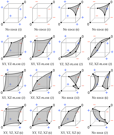
Figure 6: We depict the 64 scenarios of the edge within a trilinear region, excluding isomorph cases specifying the count within parentheses. No edge indicates where two diagonal zero corners are not connected. The labels XY, YZ, and XZ refer to $x=y$, $y=z$, and $z=x$ diagonal planes, respectively, form the shared edge, connecting the two diagonal zero corners, with the hypersurface in the schematic figure. In nearly all cases, a diagonal plane intersects with the hypersurface, except, at most, four cases, depending on the curvature determined by corner values.

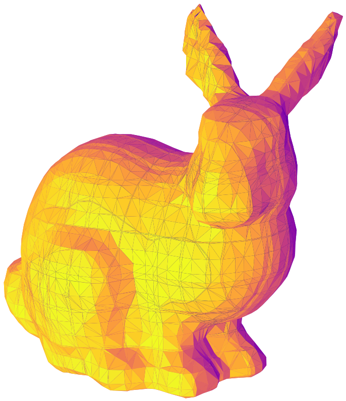
Figure 7: The normal map is analytically generated from piecewise trilinear networks, comprising both HashGrid (Müller et al., 2022) and ReLU neural networks, that have been trained to learn a signed distance function with the eikonal loss for the Stanford bunny (Curless & Levoy, 1996). Our approach dynamically assigns vertices based on the learned decision boundary. One notable observation is that the configuration of hash grids influences the selection of vertices. Additionally, each grid can be subdivided into multiple polyhedra to accurately represent smooth curves.

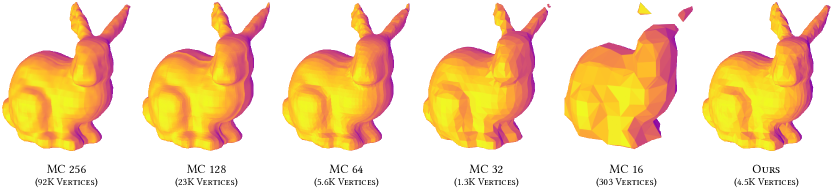
Figure 8: Visualizing normal maps for marching cubes varying the number of samplings, and ours, with the number of vertices denoted in parentheses. Low sampling has a risk of omitting sharp object details, while dense sampling results in redundant vertices and faces. As our mesh is analytically extracted from the decision boundary apex points of networks, it represents an optimal choice in balancing detail preservation and efficiency.

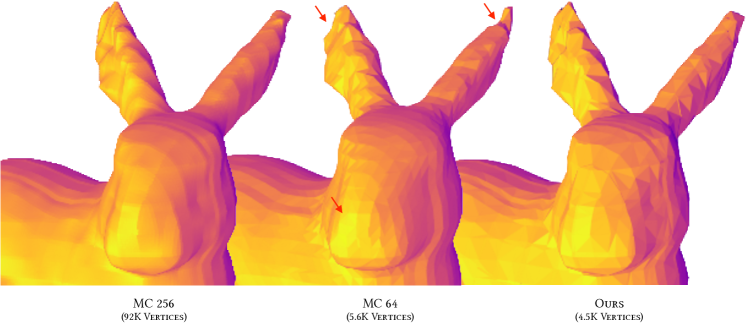
Figure 9: In a face-to-face comparison, we examine marching cubes with 256 and 64 samplings, denoted as MC 256 and MC 64, respectively, and our method. Notably, MC 64 struggles to accurately represent pointy areas of meshes due to its coarse sampling. In contrast, our approach has an advantage in this aspect, as we analytically extract the mesh from the decision boundary apex points of networks. However, it is worth noting that our adaptive sampling introduces a disadvantage where some vertices are in close proximity; specifically, we observed that 10.1% of vertices are within 1e-3 proximity to others. We believe that optimizing the mesh can significantly improve the parsimony of the vertex count compared with marching cubes.

References

- Berzins (2023) Berzins, A. Polyhedral complex extraction from relu networks using edge subdivision. In International Conference on Machine Learning. PMLR, 2023.
- Bruns (1895) Bruns, H. Das eikonal, volume 21. S. Hirzel, 1895.
- Chen et al. (2022) Chen, A., Xu, Z., Geiger, A., Yu, J., and Su, H. TensoRF: Tensorial radiance fields. In European Conference on Computer Vision, pp. 333–350. Springer, 2022.
- Curless & Levoy (1996) Curless, B. and Levoy, M. A volumetric method for building complex models from range images. In Proceedings of the 23rd annual conference on Computer graphics and interactive techniques, pp. 303–312, 1996.
- Doi & Koide (1991) Doi, A. and Koide, A. An efficient method of triangulating equi-valued surfaces by using tetrahedral cells. IEICE TRANSACTIONS on Information and Systems, 74(1):214–224, 1991.
- Edelman & Murakami (1995) Edelman, A. and Murakami, H. Polynomial roots from companion matrix eigenvalues. Mathematics of Computation, 64(210):763–776, 1995.
- Friedrich et al. (2008) Friedrich, T. et al. Elementary geometry, volume 43. American Mathematical Soc., 2008.
- Grigsby & Lindsey (2022) Grigsby, J. E. and Lindsey, K. On transversality of bent hyperplane arrangements and the topological expressiveness of relu neural networks. SIAM Journal on Applied Algebra and Geometry, 6(2):216–242, 2022.
- Gropp et al. (2020) Gropp, A., Yariv, L., Haim, N., Atzmon, M., and Lipman, Y. Implicit geometric regularization for learning shapes. arXiv preprint arXiv:2002.10099, 2020.
- Hanin & Rolnick (2019) Hanin, B. and Rolnick, D. Complexity of linear regions in deep networks. In International Conference on Machine Learning, pp. 2596–2604. PMLR, 2019.
- Hoppe et al. (1993) Hoppe, H., DeRose, T., Duchamp, T., McDonald, J., and Stuetzle, W. Mesh optimization. In Proceedings of the 20th annual conference on Computer graphics and interactive techniques, pp. 19–26, 1993.
- Humayun et al. (2023) Humayun, A. I., Balestriero, R., Balakrishnan, G., and Baraniuk, R. G. Splinecam: Exact visualization and characterization of deep network geometry and decision boundaries. In Proceedings of the IEEE/CVF Conference on Computer Vision and Pattern Recognition, pp. 3789–3798, 2023.
- Itenberg et al. (2009) Itenberg, I., Mikhalkin, G., and Shustin, E. I. Tropical algebraic geometry, volume 35. Springer Science & Business Media, 2009.
- Katz (2017) Katz, E. What is… tropical geometry. Notices of the AMS, 64(4), 2017.
- Kim et al. (2018) Kim, H., Kim, M., Seo, D., Kim, J., Park, H., Park, S., Jo, H., Kim, K., Yang, Y., Kim, Y., Sung, N., and Ha, J.-W. NSML: Meet the MLAAS platform with a real-world case study. arXiv preprint arXiv:1810.09957, 2018.
- Lei & Jia (2020) Lei, J. and Jia, K. Analytic marching: An analytic meshing solution from deep implicit surface networks. In International Conference on Machine Learning, pp. 5789–5798. PMLR, 2020.
- Lei et al. (2021) Lei, J., Jia, K., and Ma, Y. Learning and meshing from deep implicit surface networks using an efficient implementation of analytic marching. IEEE Transactions on Pattern Analysis and Machine Intelligence, 44(12):10068–10086, 2021.
- Li et al. (2023) Li, Z., Müller, T., Evans, A., Taylor, R. H., Unberath, M., Liu, M.-Y., and Lin, C.-H. Neuralangelo: High-fidelity neural surface reconstruction. In Proceedings of the IEEE/CVF Conference on Computer Vision and Pattern Recognition, pp. 8456–8465, 2023.
- Lorensen & Cline (1987) Lorensen, W. E. and Cline, H. E. Marching cubes: A high resolution 3d surface construction algorithm. ACM SIGGRAPH Computer Graphics, 21(4):163–169, 1987.
- Maclagan & Sturmfels (2021) Maclagan, D. and Sturmfels, B. Introduction to tropical geometry, volume 161. American Mathematical Society, 2021.
- Mildenhall et al. (2021) Mildenhall, B., Srinivasan, P. P., Tancik, M., Barron, J. T., Ramamoorthi, R., and Ng, R. Nerf: Representing scenes as neural radiance fields for view synthesis. Communications of the ACM, 65(1):99–106, 2021.
- Müller et al. (2022) Müller, T., Evans, A., Schied, C., and Keller, A. Instant neural graphics primitives with a multiresolution hash encoding. ACM Transactions on Graphics (ToG), 41(4):1–15, 2022.
- Raghu et al. (2017) Raghu, M., Poole, B., Kleinberg, J., Ganguli, S., and Sohl-Dickstein, J. On the expressive power of deep neural networks. In international conference on machine learning, pp. 2847–2854. PMLR, 2017.
- Serra et al. (2018) Serra, T., Tjandraatmadja, C., and Ramalingam, S. Bounding and counting linear regions of deep neural networks. In International Conference on Machine Learning, pp. 4558–4566. PMLR, 2018.
- Shen et al. (2021) Shen, T., Gao, J., Yin, K., Liu, M.-Y., and Fidler, S. Deep marching tetrahedra: a hybrid representation for high-resolution 3d shape synthesis. Advances in Neural Information Processing Systems, 34:6087–6101, 2021.
- Tancik et al. (2020) Tancik, M., Srinivasan, P., Mildenhall, B., Fridovich-Keil, S., Raghavan, N., Singhal, U., Ramamoorthi, R., Barron, J., and Ng, R. Fourier features let networks learn high frequency functions in low dimensional domains. Advances in Neural Information Processing Systems, 33:7537–7547, 2020.
- Vaswani et al. (2017) Vaswani, A., Shazeer, N., Parmar, N., Uszkoreit, J., Jones, L., Gomez, A. N., Kaiser, Ł., and Polosukhin, I. Attention is all you need. Advances in neural information processing systems, 30, 2017.
- Wang et al. (2021) Wang, P., Liu, L., Liu, Y., Theobalt, C., Komura, T., and Wang, W. Neus: Learning neural implicit surfaces by volume rendering for multi-view reconstruction. arXiv preprint arXiv:2106.10689, 2021.
- Yariv et al. (2023) Yariv, L., Hedman, P., Reiser, C., Verbin, D., Srinivasan, P. P., Szeliski, R., Barron, J. T., and Mildenhall, B. Bakedsdf: Meshing neural sdfs for real-time view synthesis. arXiv preprint arXiv:2302.14859, 2023.
- Zhang et al. (2018) Zhang, L., Naitzat, G., and Lim, L.-H. Tropical geometry of deep neural networks. In International Conference on Machine Learning, pp. 5824–5832. PMLR, 2018.
- Zhang et al. (2020) Zhang, Z., Wang, Y., Jimack, P. K., and Wang, H. Meshingnet: A new mesh generation method based on deep learning. In International Conference on Computational Science, pp. 186–198. Springer, 2020.