The physical properties of -4LAC low-synchrotron-peaked BL Lac objects
Abstract
Previous studies on the fitting of spectral energy distributions (SEDs) often apply the external-Compton process to interpret the high-energy peak of low-synchrotron-peaked (LSP) BL Lac objects (LBLs), despite the lack of strong broad emission lines observed for LBLs. In this work, we collect quasi-simultaneous multi-wavelength data of 15 LBLs from the fourth LAT AGN catalog (4LAC). We propose an analytical method to assess the necessity of external photon fields in the framework of one-zone scenario. Following derived analytical results, we fit the SEDs of these LBLs with the conventional one-zone leptonic model and study their jet physical properties. Our main results can be summarized as follows. (1) We find that most LBLs cannot be fitted by the one-zone synchrotron self-Compton (SSC) model. This indicates that external photons play a crucial role in the high-energy emission of LBLs, therefore we suggest that LBLs are masquerading BL Lacs. (2) We suggest that the -ray emitting regions of LBLs are located outside the broad-line region and within the dusty torus. (3) By extending the analytical method to all types of LSPs in -4LAC (using historical data), we find that the high-energy peaks of some flat spectrum radio quasars and blazar candidates of unknown types can be attributed to the SSC emission, implying that the importance of external photons could be minor. We suggest that the variability timescale may help distinguish the origin of the high-energy peak.
keywords:
radiation mechanisms: non-thermal – galaxies: active – galaxies: jets.1 Introduction
Blazars are the most extreme subclass of active galactic nuclei (AGNs), whose emission is dominated by the non-thermal emission from the relativistic jet orients close to observers’ line of sight (Urry & Padovani, 1995). Due to relativistic beaming effects, the observed emission is Doppler boosted, and variability timescale is shortened (e.g., Böttcher, 2019; Cerruti, 2020). The spectral energy distributions (SEDs) of blazars usually show a double-peak structure in the diagram (e.g., Böttcher, 2007). Because of the detected significant linear polarization, the low-energy peak (from radio to UV/X-ray) is attributed to synchrotron emission from relativistic electrons in a magnetic field. In leptonic scenarios, the high-energy peak (from X-ray to -ray band) is attributed to the inverse Compton (IC) scattering of relativistic electrons (e.g., Dermer, 1995; Dermer & Schlickeiser, 2002; Böttcher, 2007). The seed photons for the IC process originate from the synchrotron emission of the same population of relativistic electrons (synchrotron self-Compton, SSC; e.g., Tavecchio et al., 1998) or from external photon fields (external-Compton, EC; e.g., Ghisellini & Tavecchio, 2009), such as the accretion disk (e.g., Dermer & Schlickeiser, 1993), the broad-line region (BLR, Sikora et al., 1994; Fan et al., 2006) and the dusty torus (DT, Błażejowski et al., 2000; Sokolov & Marscher, 2005). Alternatively, the hadronic model is another possible origin of the high-energy peak (e.g., Mannheim, 1993; Dermer et al., 2012; Dimitrakoudis et al., 2012; Li et al., 2022; Xue et al., 2022, 2023; Wang et al., 2023). Based on the emission line features, blazars can be classified into BL Lac objects (BL Lacs) with no or weak emission lines (equivalent width, Å) and flat spectrum radio quasars (FSRQs) with strong emission lines ( Å; Urry & Padovani, 1995). According to the peak frequency of the low-energy synchrotron peak (), Abdo et al. (2010b) divided blazars into low-synchrotron-peaked (LSP, Hz), intermediate-synchrotron-peaked (ISP, Hz) and high-synchrotron-peaked (HSP, Hz) sources. Ajello et al. (2022) found that FSRQs are basically LSPs, while BL Lacs have a more uniform distribution of low-energy peaks. Modeling SEDs of blazars provides us a way to explore the intrinsic physical properties of emitting region inside the jet (e.g., Ghisellini & Tavecchio, 2008, 2009, 2010; Ghisellini et al., 2014; Mankuzhiyil et al., 2011; Mankuzhiyil et al., 2012; Tan et al., 2020; Deng et al., 2021; Yan et al., 2014; Zhang et al., 2012).
The conventional one-zone leptonic model has been widely applied to reproduce blazars’ SEDs. FSRQs are usually fitted with a one-zone EC model in their SEDs (e.g., Ghisellini et al., 2010; Ghisellini et al., 2014), due to the observation of broad emission lines. In contrast, the situation for BL Lacs is more complicated. ISP BL Lacs (IBLs) and HSP BL Lacs (HBLs) generally adopt a one-zone SSC model for fitting (e.g., Zhang et al., 2012; Yan et al., 2014; Ding et al., 2017), while LSP BL Lacs (LBLs) typically use the one-zone EC model (e.g., Böttcher & Bloom, 2000; Wang & Xue, 2021; Deng & Jiang, 2023). Yan et al. (2014) found that the one-zone SSC model has difficulty in explaining the SEDs of LBLs. Specifically, the model predicted low-energy peaks are higher than those suggested by the data points. Furthermore, the X-ray spectrum of some LBLs is too soft to naturally extend to the higher-energy band. Therefore it is reasonable to introduce another component to interpret the high-energy peak. In the one-zone leptonic model, an EC component is typically introduced, even though no strong broad emission lines are observed for LBLs. If the EC emission does indeed dominate the high-energy peak, then it implies that the broad emission lines of LBLs are outshone by the luminous non-thermal emission from the jet. Consequently, LBLs can be considered as masquerading BL Lacs (e.g., Giommi et al., 2012; Giommi et al., 2013; Liu et al., 2019; Xiao et al., 2022b). Therefore, it would be advantageous to explore if external photons are indispensable for interpreting the high-energy peak of LBLs.
The rapid and large-amplitude variability of blazars imply that not only the flux in each band vary dramatically, but also the peak frequencies of the double peaks shift significantly with time (e.g., Massaro et al., 2004; Sahakyan & Giommi, 2021; Zhang et al., 2012). Therefore, quasi-simultaneous multi-wavelength SEDs are essential to reveal the physical properties of their jets (e.g., Yan et al., 2014). In this work, we collect quasi-simultaneous multi-wavelength data of 15 LBLs from the fourth LAT AGN catalog (4LAC). By using an analytical method to constrain the parameter space, we analyse the applicability of the one-zone SSC model to LBLs. We explore the physical properties of LSP blazars jets by interpreting their SEDs in the framework of one-zone leptonic model. This paper is organized as follows. In Section 2, we present the sample collection and -LAT data analysis. The analytical method and model description are given in Section 3, followed by the results and discussion in Section 4. Finally, we end with conclusions in Section 5. The cosmological parameters , , and = 0.71 (Bennett et al., 2014) are used throughout this work.
2 sample collection and data analysis
2.1 Sample collection
We collected 15 LBLs from -4LAC as our sample. To obtain their contemporaneous multi-wavelength SEDs, we firstly collected all data and corresponding observation times of these LBLs in the Space Science Data Center (SSDC) SED Builder (Stratta et al., 2011)111http://tools.ssdc.asi.it/SED/. Then, we searched for the intersection of observation time in the infrared to X-ray range and ensured that the time interval between any two bands does not exceed seven days. The radio data were not taken into account, because they could not be explained by a one-zone model and the radio data available on the SSDC were mostly collected around the 1990s. Finally, we obtained the GeV data by integrating two months that include the previous time intersection (details can be found in Section 2.2), because the -ray data on the SSDC are obtained by integrating annually, which obviously does not meet the requirement of contemporaneous multi-wavelength data. Note that the observation time intervals of the data from infrared to X-ray range that we collected are within one week, while the -LAT data are integrated for two months. Therefore, the multi-wavelength data in this sample are quasi-simultaneous rather than simultaneous. The details of the quasi-simultaneous data of each LBL are given in Table 1.
2.2 Fermi-LAT data analysis
The LAT on board the Fermi mission is a pair-conversion instrument that is sensitive to GeV emission (Atwood et al., 2009). We collected Fermi-LAT data in the sky-survey mode encompassing two months listed as in Table 1, which is taken from the Table 1 as the midpoint. Data were analyzed with the fermitools version 2.2.0. A binned maximum likelihood analysis was performed on a region of interest (ROI) with a radius centered on the “R.A.” and “decl.” of each source. Recommended event selections for data analysis were “FRONT+BACK” (evtype=3) and evclass=128. We applied a maximum zenith angle cut of to reduce the effect of the Earth albedo background. The standard gtmktime filter selection with an expression of (DATA_QUAL LAT_CONFIG ) was set. A source model was generated containing the position and spectral definition for all the point sources and diffuse emission from the 4FGL (Abdollahi et al., 2022) within of the ROI center. The analysis included the standard galactic diffuse emission model () and the isotropic component (iso_P8R3_SOURCE_V3_v1.txt), respectively. We binned the data in counts maps with a scale of per pixel and used 30 logarithmically spaced bins in energy of GeV. The energy dispersion correction was made when event energies extending down to 100 MeV were taken into consideration. We divide this spectral energy distribution into six or three equal logarithmic energy bins in the GeV for sources above or below , respectively, shown in Fig. 2. The data points with or nominal flux uncertainty larger than half the flux itself are given upper limits at the 95% confidence level.
| name | Source name | RA (J2000) | Dec. (J2000) | |||
|---|---|---|---|---|---|---|
| (degrees) | (degrees) | |||||
| (1) | (2) | (3) | (4) | (5) | (6) | (7) |
| 4FGL J0100.3+0745 | GB6 J0100+0745 | 0.30052 | 15.0866 | 7.7643 | 2010.07.09 | 2010.06.09–2010.08.09 |
| 4FGL J0141.4-0928 | PKS 0139-09 | 0.733 | 25.357634 | -9.478798 | 2010.05.30–2010.06.06 | 2010.05.03–2010.07.03 |
| 4FGL J0210.7-5101 | PKS 0208-512 | 1.003 | 32.692502 | -51.017193 | 2009.11.26 | 2009.10.26–2009.12.26 |
| 4FGL J0238.6+1637 | PKS 0235+164 | 0.94 | 39.662209 | 16.616465 | 2010.01.30 | 2010.01.01–2010.03.01 |
| 4FGL J0334.2-4008 | PKS 0332-403 | 1.445 | 53.556894 | -40.140388 | 2010.01.17–2010.01.18 | 2009.12.17–2010.02.17 |
| 4FGL J0522.9-3628 | PKS 0521-36 | 0.055 | 80.741603 | -36.45857 | 2010.03.05 | 2010.02.05–2010.04.05 |
| 4FGL J0854.8+2006 | PKS 0851+202 | 0.306 | 133.703646 | 20.108511 | 2010.04.10 | 2010.03.10–2010.05.10 |
| 4FGL J0958.7+6534 | S4 0954+65 | 0.367 | 149.696855 | 65.565228 | 2010.03.12 | 2010.02.12–2010.04.12 |
| 4FGL J1043.2+2408 | B2 1040+24A | 0.559117 | 160.787649 | 24.143169 | 2010.07.09 | 2010.06.09–2010.08.09 |
| 4FGL J1147.0-3812 | PKS 1144-379 | 1.048 | 176.755711 | -38.203062 | 2010.06.24 | 2010.05.24–2010.07.24 |
| 4FGL J1517.7-2422 | AP Lib | 0.048 | 229.424223 | -24.372078 | 2010.02.20 | 2010.01.20–2010.03.20 |
| 4FGL J1751.5+0938 | OT 081 | 0.322 | 267.886744 | 9.650202 | 2010.04.01 | 2010.03.01–2010.05.01 |
| 4FGL J1800.6+7828 | S5 1803+784 | 0.68 | 270.190349 | 78.467783 | 2009.10.13 | 2009.09.13–2009.11.13 |
| 4FGL J2152.5+1737 | S3 2150+17 | 0.871 | 328.137 | 17.6173 | 2010.04.08–2010.04.10 | 2010.03.09–2010.05.09 |
| 4FGL J2247.4-0001 | PKS 2244-002 | 0.949 | 341.867 | -0.0263 | 2010.01.14–2010.01.16 | 2009.12.15–2010.02.15 |
3 Analytical method and model description
The following analytical method and numerical modeling are carried out within the framework of the one-zone leptonic model. It is assumed that all the radiation of the blazar jet comes from a spherical emitting region with radius , which is filled with a uniform magnetic field and a plasma of charged particles. The emitting region moves along a relativistic jet with the bulk Lorentz factor at a viewing angle to the observer’s line of sight, where is the speed of the emitting region. Due to relativistic beaming effects, the observed flux is boosted by a factor of , where is the Doppler factor. In this paper, we approximate by assuming . In this section, parameters without superscript are measured in the comoving frame, those with superscript "obs" are measured in the frame of the observer, and those with superscript "AGN" are measured in the AGN frame, unless specified otherwise.
3.1 Analytical method
In order to explore the necessity of external photon fields, the following analytical calculation of searching the parameter space will be carried out under the one-zone SSC model. In the one-zone model, the physical properties of the emitting region are characterized by three parameters, i.e., , , and , which can be constrained analytically based on the peak frequencies and peak luminosities of two SED peaks (Chen, 2017, 2018). Here we adopt – cm, 0.1–10 G (e.g., O’Sullivan & Gabuzda, 2009; Pushkarev et al., 2012; Karamanavis et al., 2016; Hodgson et al., 2017; Kang et al., 2021; Kim et al., 2022), and 1–30 (Hovatta et al., 2009) as the reference ranges for , , and suggested by observations (hereafter referred to as the observational constraints). If no parameter space could be found within them, introducing the external photon field to explain the high-energy peak would be inevitable.
From peak frequencies of the two peaks, the relation between and can be obtained. In the framework of one-zone SSC model, the emission at the peak frequency is dominantly produced by relativistic electrons with , where is the break Lorentz factor of the electron energy distribution (EED). Using the monochromatic approximation (Rybicki & Lightman, 1979a), the peak frequency of low-energy peak can be expressed as
| (1) |
where is the redshift. In the Thomson (TMS) regime, the peak frequency of the high-energy peak is expressed as . Combining them together, the relation between and can be obtained
| (2) |
It can be seen that when and are derived from observation, and are inversely proportional. Since the frequency obtained by the empirical function has some uncertainty, we consider an uncertainty of a factor of 3 in in the following.
The relation between , , in the TMS regime can also be obtained from the ratio of the total luminosities of the two peaks,
| (3) |
where and represent the total luminosities of the IC peak and the synchrotron peak, respectively; and are the energy densities of synchrotron photons and magnetic field in the comoving frame, respectively, where is the speed of light. If assuming that the shape of two peaks can be represented by a broken power law spectrum, we have
| (4) |
where is the peak luminosity, and is a correction term, where and are the slopes below and above the peaks, respectively, in the diagram. Substituting Eq. (4) into Eq. (3), we have
| (5) |
where and are the peak luminosities of the low-energy peak and the high-energy peak, respectively. If considering satisfies the observational constraint, the correlation between and can be obtained. Combining Eq. (2) and Eq. (5), it is possible to find that if a reasonable parameter space can be found in one-zone SSC model for LBLs under the TMS regime.
On the other hand, since the high-energy peaks of LBLs usually extend to band, it is necessary to check if the Klein–Nishina (KN) effect becomes severe and softens the spectrum. When and satisfy
| (6) |
where is the Planck constant, and is the electron rest mass, the KN effect will be severe, lowering the peak frequency and peak luminosity of the IC peak. Following Tavecchio et al. (1998), in the KN regime can be obtained by
| (7) |
where . Combining Eq. (1) and Eq. (7), we can get the relation between and
| (8) |
Interestingly, in the KN regime, the relation between and turns to be positive, which indicates that the parameter spaces constrained in the TMS regime and the KN regime will be quite different.
Due to the severe KN effect, the IC cooling efficiency is greatly reduced, so the ratio of the total luminosity needs to be corrected as
| (9) |
where is the available energy density of synchrotron photons, which can be obtained by integrating the energy density of photons with frequency , i.e.,
| (10) |
Substituting Eq. (4), Eq. (7), and Eq. (10) into Eq. (9), we can obtain the relation between , , and in the KN regime as
| (11) |
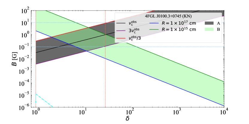
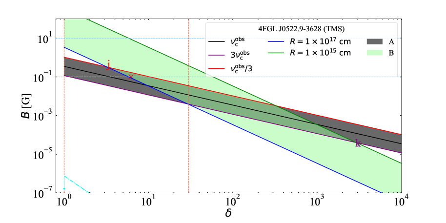
Finally, we can analyse the applicability of the one-zone SSC model to LBLs in different scattering regimes. Here, we take the first LBL of our sample, i.e., 4FGL J0100.3+0745, as an example to show its parameter space derived with above methods. The resulting parameter spaces are shown in Fig. 1, where the upper panel is for the KN regime, and the lower panel is for the TMS regime. Combining Eq. (1) and Eq. (6), we can find that only when
| (12) |
the severe KN effect will be triggered. Therefore, the space above the cyan dash-dotted line in the upper panel of Fig. 1 should be discarded. Since no parameter space can be found under the observational constraints (corresponding to the rectangular region), we suggest that its SED cannot be fitted with the one-zone SSC model in the KN regime. To explore the possibility of reproducing SEDs in the KN regime for general cases, we give a test in the critical condition (, ). By setting (an average value suggested by Ackermann et al., 2011), we find that only when Hz, there is a intersect area between the cyan dash-dotted line and the rectangular region. Therefore, for LBLs, we only need to consider whether there is a parameter space satisfying observational constraints in the TMS regime. However, it can be seen from the lower panel of Fig. 1 that there is still no parameter space. Therefore, the external photon field is necessary to be introduced. The above analytical methods would be applied in this work and the corresponding results would be given in Section 4.

3.2 Model description
The external photon fields in the mostly applied one-zone EC model are BLR and DT, which are closely related to the thermal radiation of the accretion disk. In our modeling, we assume that the accretion disk is geometrically thin and optically thick (Shakura & Sunyaev, 1973). Its emission profile has the following multi-temperature blackbody form (Frank et al., 2002):
| (13) |
where is the luminosity distance, is the Boltzmann constant, is the radial distance between the disk and the central supermassive black hole (SMBH), and are the inner and outer radii of the disk, assumed to be and , respectively (e.g., Frank et al., 2002), where is the Schwarzschild radius, is the universal gravitational constant, is the mass of the SMBH. Note that, only affects the peak frequency of the thermal radiation of the accretion disk. For simplicity, is assumed to be an average value of solar mass (Paliya et al., 2017; Xiao et al., 2022a). The radial dependence of the temperature is as follows:
| (14) |
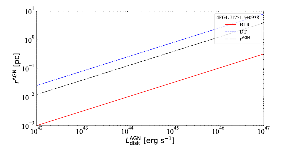
where is the luminosity of the accretion disk, is the Stefan-Boltzmann constant, is the accretion efficiency (e.g., Paliya et al., 2017). Since the emitting region is moving away from the accretion disk, the energy density of rear-end photons from the disk is usually low in the comoving frame. Therefore, in this work, we mainly consider the BLR and DT as the external photon fields (e.g., D’Ammando et al., 2016; Arsioli & Chang, 2018), which reprocess of the disk luminosity into the BLR and DT radiation, respectively (e.g., Hayashida et al., 2012). The energy densities of the BLR () and the DT () in the comoving frame can be estimated as (Hayashida et al., 2012)
| (15) |
and
| (16) |
where is the distance between the emitting region and the SMBH, pc and pc are the characteristic distances of the BLR and DT, respectively (e.g., Ghisellini & Tavecchio, 2008). The radiation of the BLR and DT are assumed to be isotropic graybody radiation, whose peak frequencies in the comoving frame are Hz (Tavecchio & Ghisellini, 2008) and Hz (Cleary et al., 2007), respectively.
In the leptonic model, the jet’s non-thermal emission is from the relativistic elections, whose distribution can be obtained by solving the continuity equation that includes injection, radiative cooling and escape (e.g., Chiaberge & Ghisellini, 1999; Hu et al., 2023). In this work, relativistic electrons are assumed to be injected into the emitting region with a broken power-law distribution at a constant rate (Ghisellini et al., 2010), i.e.,
| (17) |
where is the electron Lorentz factor, and are the minimum and maximum electron Lorentz factors, respectively, and are the spectral indices below and above , respectively, is a normalization constant in units of , which can be obtained from , where is the electron injection luminosity. When the injection is balanced by the cooling and escape (Deng et al., 2021; Chiaberge & Ghisellini, 1999; Li & Kusunose, 2000; Böttcher & Chiang, 2002; Tramacere et al., 2011; Yan et al., 2012), the steady-state EED is obtained as where . More specifically, is the dynamical timescale, and is the radiative cooling timescale, where is the Thomson scattering cross-section,
| (18) | ||||
is a numerical factor accounting for the KN effect (e.g., Schlickeiser & Ruppel, 2010; Xue et al., 2022), where is the energy of soft photons, , is the number density distribution of soft photons, is the energy density of soft photons. For SSC model, we set , while for EC model.
After obtaining the steady-state EED , we can calculate the non-thermal radiation of the jet, including synchrotron, SSC, and EC emissions. For the synchrotron emission, its emission coefficient can be obtained by
| (19) |
where is the mean emission coefficient for a single electron integrated over the isotropic distribution of pitch angles (e.g., Crusius & Schlickeiser, 1986; Ghisellini et al., 1988; Katarzyński et al., 2001). And the synchrotron absorption coefficient (e.g., Rybicki & Lightman, 1979b) can be calculated with
| (20) |
Then, we can calculate the synchrotron intensity by solving radiative transfer equation for the spherical geometry (e.g., Bloom & Marscher, 1996; Kataoka et al., 1999):
| (21) |
where is the optical depth.
The SSC and EC emission coefficients are given as
| (22) |
where and are the soft photon energy and the scattered photon energy in units of , respectively, is the number density of soft photons per energy interval, is the Compton kernel given by Jones (1968). Since the emitting region is transparent for IC radiation, we can obtain the IC intensity as Finally, the total observed flux density of the jet can be calculated by
| (23) |
Due to the possibility of annihilation between high-energy photons and low-energy photons, we calculate the internal absorption (e.g., Dermer & Menon, 2009) and correct the GeV–TeV spectrum by using the extragalactic background light model presented by Saldana-Lopez et al. (2021).
There are 11 free parameters in our model: , , , , , , , , , , and only for the EC model. Since they are coupled to each other, reproducing the best-fit SEDs will take a long time if we allow all parameters to be free. In this work, we estimate and from the spectral indices and of the SEDs, respectively. We set , because it has little effect on the fitting results. We adopt (Ghisellini et al., 2005) as a default value, unless it is constrained by the quasi-simultaneous data of the low-energy peak (e.g., Zhang et al., 2012). Finally, we determine by fitting the optical-UV data if there is a blue bump structure, otherwise we assume that can be any value that does not contaminate the synchrotron emission.
| Source name | |||||||||||
|---|---|---|---|---|---|---|---|---|---|---|---|
| (G) | (cm) | () | () | (pc) | |||||||
| (1) | (2) | (3) | (4) | (5) | (6) | (7) | (8) | (9) | (10) | (11) | (12) |
| 4FGL J0100.3+0745 | 29.0 | 1.0 | 16.8 | 39.8 | 2.7 | 0.1 | 3.1 | 6.3 | 42.5 | -2.2 | 6.1 |
| 4FGL J0141.4-0928a | 9.7 | 1.0 | 16.7 | 43.3 | 2.6 | 1.0 | 2.5 | 4.0 | 43.9 | -1.5 | 7.5 |
| 4FGL J0210.7-5101a | 18.5 | 2.0 | 16.4 | 42.8 | 2.8 | 1.2 | 3.9 | 3.2 | 46.2 | -0.4 | 13.4 |
| 4FGL J0238.6+1637ab | 15.1 | 0.8 | 16.6 | 43.0 | 2.7 | 0.7 | 3.7 | 3.6 | 43.9 | -1.4 | 141.6 |
| 4FGL J0334.2-4008ab | 26.0 | 0.5 | 16.9 | 42.8 | 2.8 | 1.5 | 2.9 | 3.8 | 43.9 | -0.8 | 34.3 |
| 4FGL J0854.8+2006ab | 11.7 | 0.9 | 16.9 | 42.9 | 2.7 | 1.1 | 2.6 | 4.3 | 43.9 | -1.2 | 82.2 |
| 4FGL J0958.7+6534b | 16.0 | 1.0 | 16.6 | 42.3 | 2.8 | 0.9 | 4.2 | 6.3 | 43.9 | -1.3 | 36.4 |
| 4FGL J1043.2+2408b | 16.0 | 1.5 | 16.4 | 42.3 | 2.6 | 0.7 | 4.5 | 6.3 | 45.2 | -0.9 | 14.4 |
| 4FGL J1147.0-3812a | 25.8 | 0.3 | 16.9 | 42.9 | 2.2 | 1.2 | 3.0 | 4.0 | 43.5 | -0.8 | 19.6 |
| 4FGL J1517.7-2422a | 4.8 | 0.3 | 16.6 | 42.9 | 3.4 | 1.8 | 2.9 | 4.9 | 43.0 | -1.6 | 35.9 |
| 4FGL J1751.5+0938b | 11.7 | 0.3 | 17.0 | 43.3 | 2.6 | 1.8 | 3.2 | 6.3 | 43.7 | -1.1 | 68.9 |
| 4FGL J1800.6+7828a | 17.9 | 1.0 | 16.6 | 42.7 | 3.3 | 1.6 | 3.7 | 4.2 | 43.2 | -1.6 | 8.9 |
| 4FGL J2152.5+1737 | 26.3 | 0.6 | 16.7 | 42.0 | 3.3 | 1.5 | 4.7 | 6.3 | 43.9 | -1.1 | 14.5 |
| 4FGL J2247.4-0001 | 16.5 | 0.5 | 16.7 | 42.7 | 3.4 | 1.7 | 3.6 | 6.3 | 43.9 | -1.3 | 5.3 |
| 4FGL J0522.9-3628b (EC) | 5.0 | 0.3 | 16.8 | 43.1 | 3.1 | 1.5 | 3.1 | 6.3 | 43.0 | -1.5 | 68.6 |
| 4FGL J0522.9-3628b (SSC) | 6.2 | 0.1 | 17.0 | 43.3 | 3.4 | 1.6 | 3.8 | 6.3 | 43.0 | 82.8 |
- Notes.
-
a
The source with limited .
-
b
The source with potentially more than one state of quasi-simultaneous data points in the optical and/or X-ray bands.
4 Results and discussion
4.1 The physical properties of LBLs
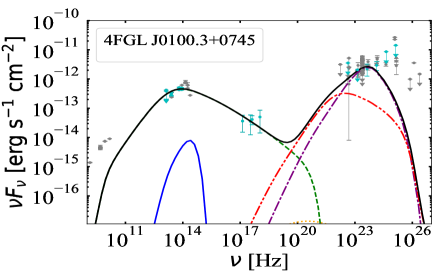
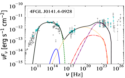
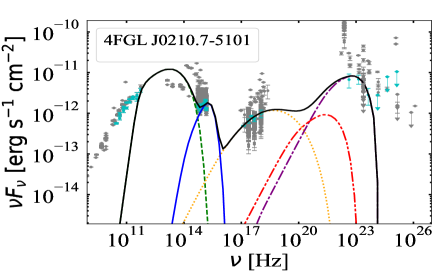
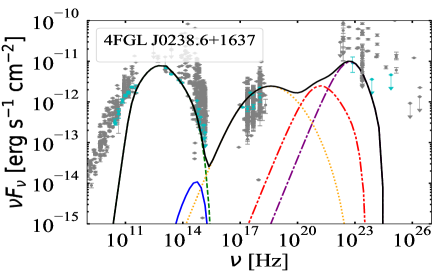
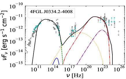
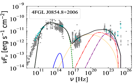
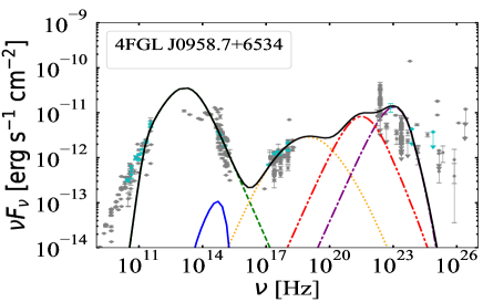
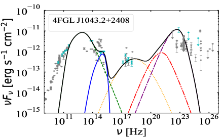
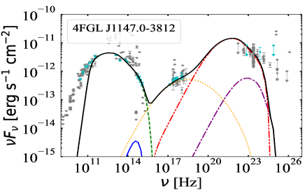
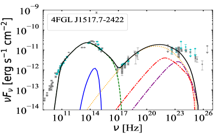
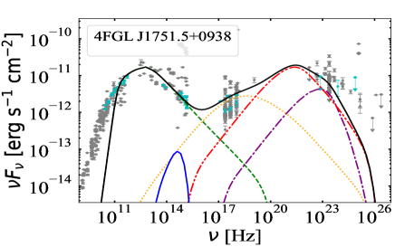
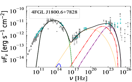
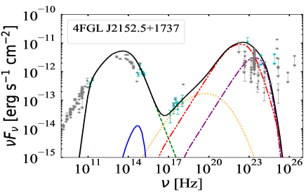
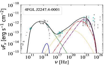
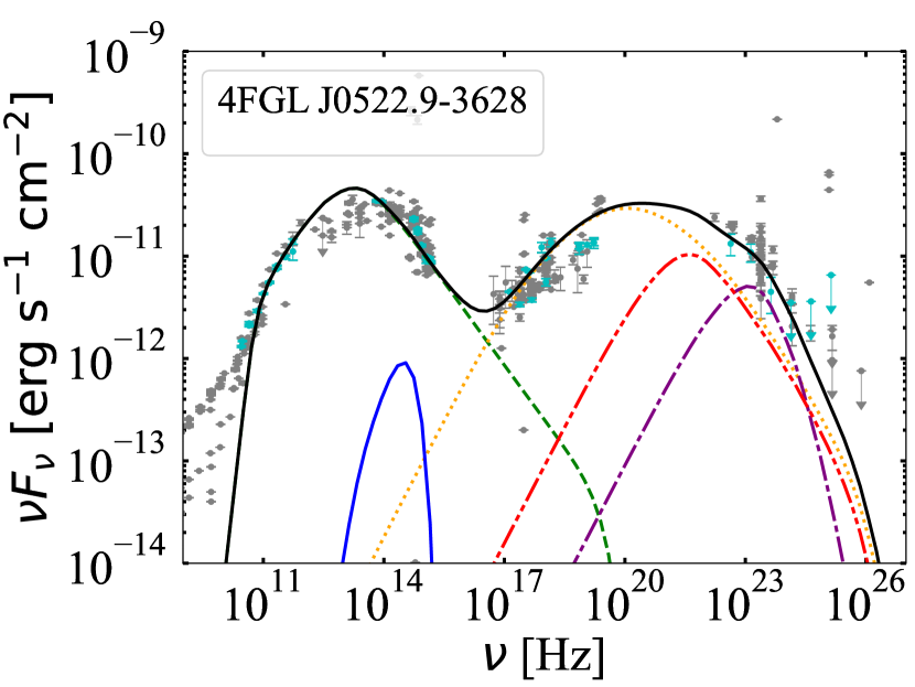
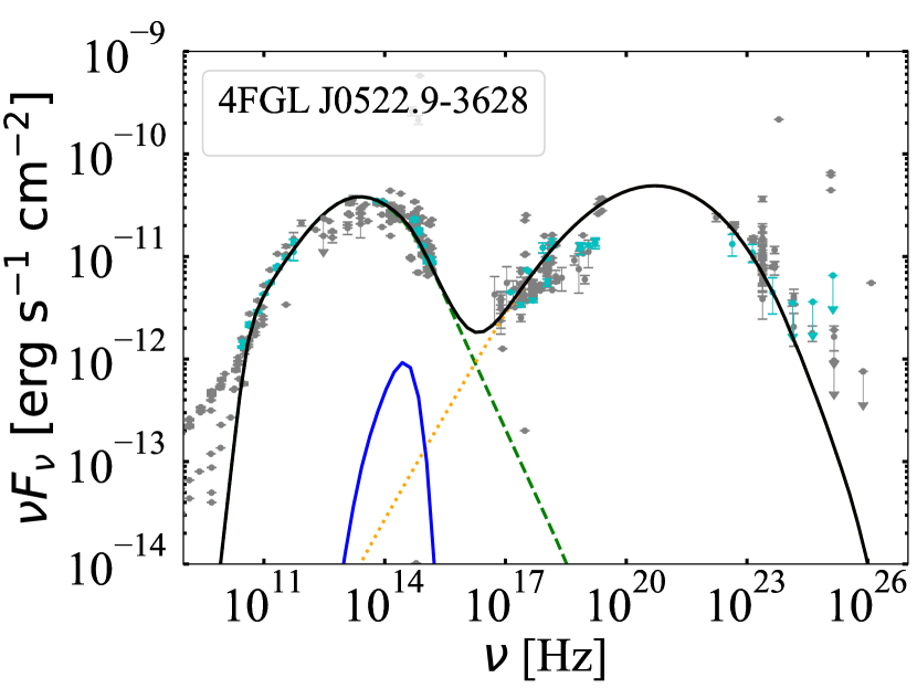
By applying the analytical method to all 15 LBLs in our sample, we find that except for 4FGL J0522.9-3628, the quasi-simultaneous multi-wavelength SEDs of the rest sources cannot be fitted with the one-zone SSC model. This indicates the importance of external photon fields for the high-energy emission of LBLs. Combining the observational feature that BL Lacs lack strong emission lines, our results suggest that LBLs may be the masquerading BL Lacs, whose broad emission lines are outshone by the non-thermal radiation of the jet (Giommi et al., 2013; Padovani et al., 2019; Xiao et al., 2022b). The fitting results with the one-zone EC model are shown in Fig. 2, and the fitting parameters are presented in the upper part of Table 2. For the modeling of 4FGL J0522.9-3628, the upper panel of Fig. 3 shows its fitting result with the conventional one-zone EC model, while the middle panel shows the parameter space of the one-zone SSC model in the TMS regime. As indicated by the derived parameter space, we fit the SED with the one-zone SSC model. The fitting result is shown in the lower panel of Fig. 3, and the parameters used for fitting are presented in the lower part of Table 2, where and are selected from the middle panel (corresponding to the red cross). It can be seen that the one-zone SSC model can fit the SED well even without external photon fields. However, this is a rare occurrence (only 1 out of 15 sources in our sample).
Due to the constraint of quasi-simultaneous observational data (see Fig. 2), as shown in Table 2, the sources with superscript "a" have less than 6.3 (corresponding to ), which implies relatively slow shock speeds. In the framework of diffusive shock acceleration mechanism, by equating (corresponding to ) with the acceleration timescale (e.g., Rieger et al., 2007; Xue et al., 2019), we can estimate the shock speed measured in the upstream frame as . Then, we find that in units of for the sources with superscript "a" in Table 2 are -3.5, -4.2, -4.0, -3.8, -3.4, -3.7, -2.9, and -3.4, from top to bottom, respectively. On the other hand, as can be seen from Table 2, sources marked with a superscript "b" have relative large values, which are due to the fact that their collected optical and/or X-ray bands quasi-simultaneous data points are rather scattered. It indicates that the quasi-simultaneous data collected from these sources within a week exhibits multiple states, including at least one flare. In the modeling, we selected the ones with shorter error bars for fitting throughout this work, which are more creditable.
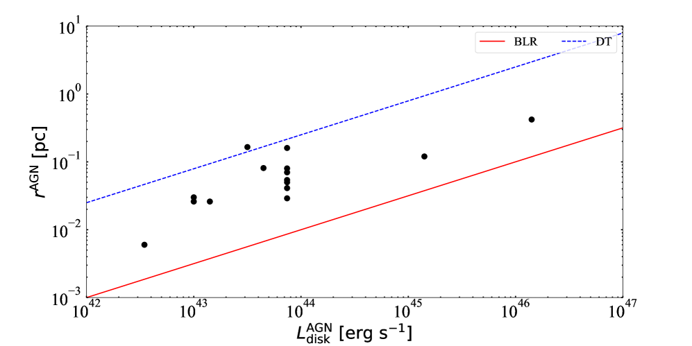
The location of the emitting region is one of the essential properties in blazars, which can be explored by investigating the dominant ambient photon fields for the EC process (e.g., Agudo et al., 2011; Dotson et al., 2012; Nalewajko et al., 2014; Böttcher & Els, 2016). However, the location of the blazar -ray emitting region is still controversial (Madejski & Sikora, 2016). Following previous studies (e.g., Dermer et al., 2009; Ghisellini & Tavecchio, 2009; Georganopoulos et al., 2012; Zdziarski et al., 2012; Yan et al., 2018), we constrain the location of the emitting region by fitting the quasi-simultaneous SEDs of 15 LBLs in -4LAC with the one-zone leptonic model. The distance () between the emitting region and the SMBH is presented in Table 2, which is determined by combining Eq. (15) and Eq. (16) to reproduce the -ray spectrum based on the assumption that the energy density of the external photon fields are functions of . In the upper panel of Fig. 4, we plot as a function of for all 15 sources in our sample. It can be seen that most LBLs have their -ray emitting regions located outside the BLR and within the DT. On the other hand, it can be found that the soft photons for the EC radiation of 8 LBLs are dominated by that from the BLR and the soft photons of other 7 LBLs are dominated by that from DT (see Fig. 2 and Fig. 3). Therefore, our modeling results suggest that the -ray emitting regions of LBLs are located inside the DT and close to the characteristic distance of BLR.
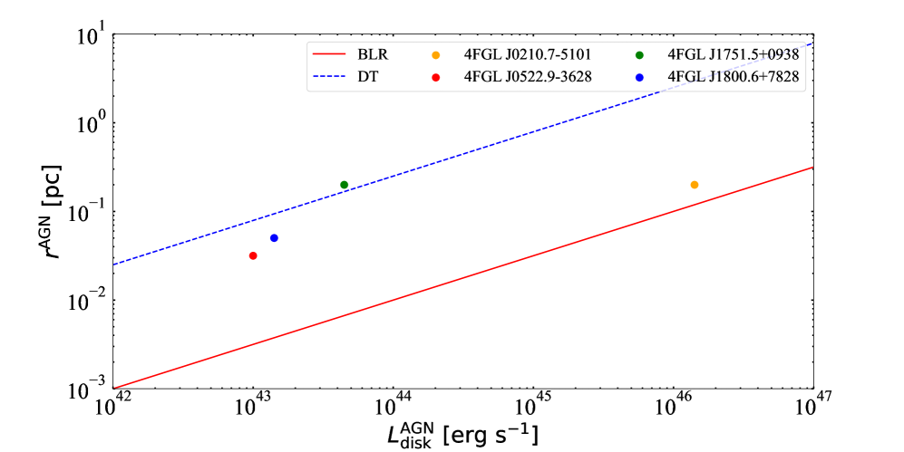
To test the above results on the location of the emitting region, it might be possible to use the variability timescale to diagnose the emitting region as well (e.g., Abdo et al., 2010a; Jorstad et al., 2010; Tavecchio et al., 2010; Liu et al., 2011; Agudo et al., 2012; Grandi et al., 2012; Brown, 2013; Ramakrishnan et al., 2015). Based on the causality relation, we have , where is the variability timescale. On the other hand, in the framework of the conical jet model, we have , where is the semi-aperture angle, assumed to be 0.1 for all sources (e.g., Ghisellini et al., 2010). By setting (a typical value suggested by observations; Hovatta et al., 2009), and taking advantage of the variability timescale (the minimum -ray variability timescales for some individual objects in our sample) from Vovk & Neronov (2013), we find that in units of pc for 4FGL J0210.7-5101, 4FGL J0522.9-3628, 4FGL J1751.5+0938, and 4FGL J1800.6+7828 are -0.7, -1.5, -0.7, and -1.3, respectively. The distribution of their emitting region locations is shown in the middle panel of Fig. 4. Since the thermal radiation of the accretion disk may be outshone by the luminous non-thermal radiation from the jet, the adopted value of can affect the location of the emitting region. Here we take 4FGL J1751.5+0938 (this source is located inside the DT in the upper panel of Fig. 4 and is marked as a green point in the middle panel of Fig. 4) as an example to show the relation between and . The corresponding result is shown in the lower panel of Fig. 4. It can be found that, when remains unchanged, there is a positive correlation between and . Therefore, if the variability timescale corresponds to the SED we collected, the difference in the distribution of 4FGL J1751.5+0938 in the upper panel and the middle panel may indicate an underestimation of . And we suggest that the -ray emitting regions of LBLs are still located outside the BLR and within the DT, i.e., the conclusion should remain unchanged.
The distribution of the emitting region locations may also be roughly explained from the perspective of the KN effect. More specifically, since the soft photons from BLR have higher energy, the corresponding EC emission will be suppressed by the KN effect earlier (e.g., Cao & Wang, 2013), leading to a steep spectrum when , where is the peak frequency of the external photon field emission. However, if the soft photons come from DT, we have , which is normally not important for LSPs. Due to the lack of KN features in the broadband spectra of bright blazars (e.g., Sikora et al., 2009), the emitting region needs to be outside the BLR.
Our results are consistent with many previous works. For example, Tan et al. (2020) modelled the quasi-simultaneous SEDs of 60 -4LAC FSRQs and suggested that most of the -ray emitting regions are located outside the BLR and within the DT. Chen & Bai (2011) proposed that the IR external photon field may play an important role by analyzing the ratio of EC to synchrotron luminosity for a sample of bright blazars, implying that the emitting regions should be outside the BLR and within the DT. Moreover, if the -ray emitting regions are inside the BLR, a feature of cutoff compatible with the interaction with BLR photons is expected in the high-energy band. However, only 10% of the broad-line blazars show the matching attenuation (Costamante et al., 2018). Therefore, the -ray emission should be produced outside the BLR most of the time.
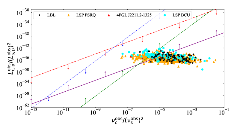
4.2 The physical properties of LSPs
As we can see from the middle panel of Fig. 3 that at least four conditions, i.e., , , , , are required to find the parameter space under the observational constraints. Combining Eq. (2) and Eq. (5), and can be expressed as
| (24) |
and
| (25) |
respectively. Here we set , because it has little effect on the results. Then, the sources and the above conditions can be represented as points and regions in the diagram, respectively. Since the analytical method is independent of the specific subclass of blazar, we can apply it to all types of LSPs in -4LAC to explore their intrinsic physical properties. To apply the above method, the values of peak frequency and peak luminosity are needed. Fortunately, Yang et al. (2022, 2023) have constructed the historical SEDs of all 750 FSRQs and 844 BL Lacs with measured redshift in the Fourth -LAT 12-year Source catalog (Abdollahi et al., 2022), and fitted them with a parabolic equation, enabling the derivation of the peak frequency and peak luminosity. Taking advantage of the archival data, we show the above constraints and the distribution of LSPs in Fig. 5. It can be seen that most of the LBLs cannot satisfy these constraints simultaneously. This implies that the external photon field is more important for LBLs than for IBLs and HBLs, which is consistent with the conclusion of Zhang et al. (2014). Therefore, our results suggest that LBLs should be masquerading BL Lacs. On the other hand, since the IC process of the external photon field will significantly increase the total luminosity of the blazar and the ratio of (e.g., Zhang et al., 2012), we suggest that the LBLs should be more Compton dominated than HBLs (e.g., Yan et al., 2014), and have higher luminosity, which is consistent with the blazar sequence (e.g., Fossati et al., 1998; Meyer et al., 2011; Ghisellini et al., 2017).
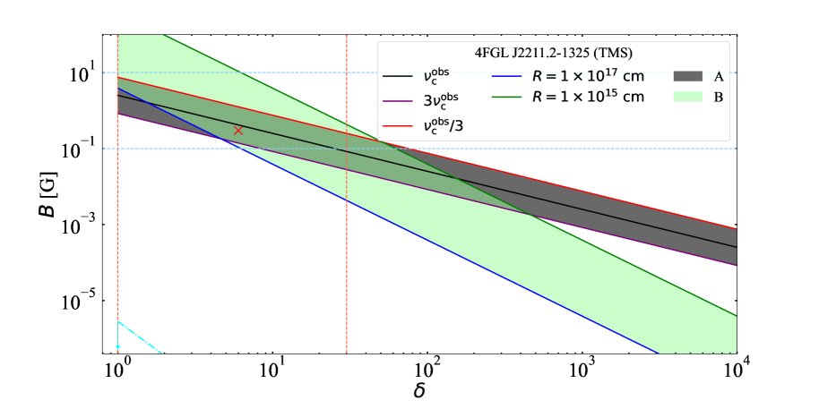
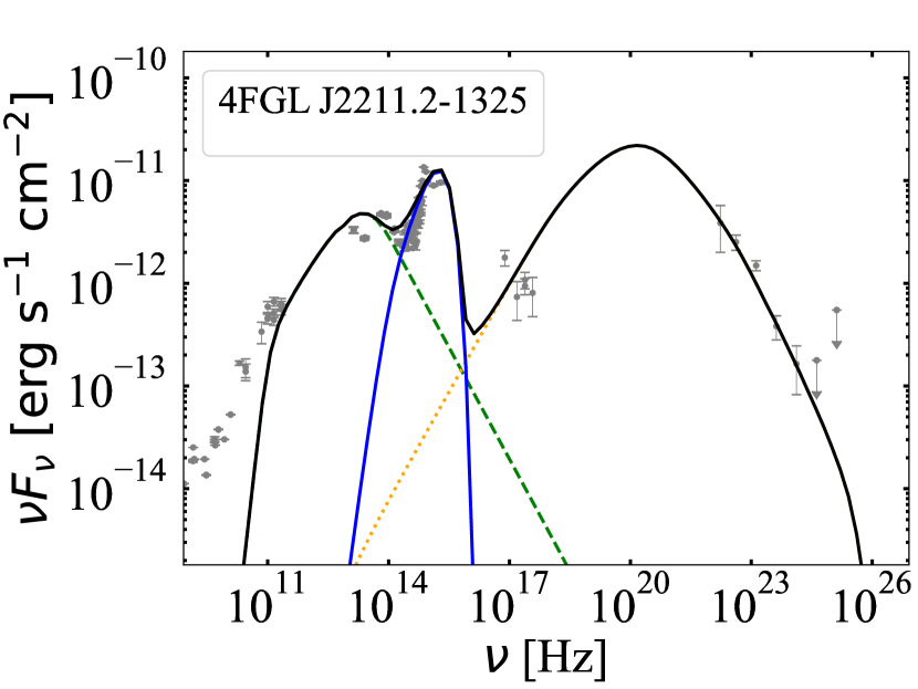
Interestingly, Fig. 5 shows that the high-energy peak of some FSRQs can be explained by the SSC emission. In order to illustrate this fact better, we take 4FGL J2211.2-1325 as an example (randomly selected from the sample), we show its parameter space under the TMS regime and fitting results with the one-zone SSC model in the upper and lower panels of Fig. 6, respectively. It can be seen that the importance of the external photon field for FSRQs can be low, which indicates that the emitting region may be located far from the SMBH, and this can be tested by the variability timescale as mentioned before.
Since the same population of relativistic electrons produce the SSC and EC emissions in the one-zone EC model, we have , where is the peak frequency of the EC emission. Combining Eq. (1), we can obtain . On the other hand, for the case of the one-zone SSC model, can be expressed as , according to Eq. (2). Since has little effect on the results, and LBLs and FSRQs have the same , the difference in the distribution of LBLs and FSRQs shown in Fig. 5 indicates that when the one-zone SSC model is applicable, FSRQs have larger , otherwise FSRQs have smaller . In addition, we can also find in Fig. 5 that the distribution of blazar candidates of unknown types (BCUs) is similar to that of FSRQs.
4.3 Variability timescale and the determination of high-energy peak origin
Normally, the variability timescale (e.g., Abdo et al., 2010a; Jorstad et al., 2010; Tavecchio et al., 2010; Liu et al., 2011; Agudo et al., 2012; Grandi et al., 2012; Brown, 2013; Ramakrishnan et al., 2015) may be a useful indicator to the location of emitting region and the origin of the high-energy peak. When the BLR and DT are taken into account, i.e., , in order to explain the high-energy peak with the SSC emission, must be satisfied. Here, we take 4FGL J0522.9-3628 as an example to explore the conditions for the applicability of the one-zone SSC model. For simplicity, we assume that the IC scattering occurs in the TMS regime, then is required when , and for the case of . Then, we find that the SSC emission can only dominate the high-energy peak when . In that case, the contribution of the EC emission to the spectrum is negligible. Therefore, our results suggest that the one-zone SSC model is only possible to be used to interpret the observed SEDs in the case of relatively long variability timescale. It should be noted that the reference range of the variability timescale mainly depends on the range of . Since the value of is mainly affected by the ratio of , which can vary greatly among different sources, there may be large differences between the thresholds of the variability timescale for different sources. Therefore, it is possible that the source with the shortest variability timescale, such as 4FGL J0522.9-3628 in the middle panel of Fig. 4, can be fitted with a one-zone SSC model, while the sources with longer variability timescales can only be fitted with a one-zone EC model. However, the variability timescale of 4FGL J0522.9-3628 used to estimate the location of the -ray emitting region is only 0.43 days. It seems to be inconsistent with our conclusion. However, it should be noted that Vovk & Neronov (2013) only presented the minimum -ray variability timescales, which may correspond to different SEDs from those we collected. Since the analytical results depend on the peak frequency and peak luminosity, the parameter space that satisfies the observational constraints in the TMS regime may not be found anymore. More specifically, for 4FGL J0522.9-3628, we believe that the high-energy peak should originate from the EC emission due to the short variability timescale, resulting in a larger , thus locating outside the region that can satisfy four conditions simultaneously (see Fig. 5). Therefore, its SED may cannot be fitted by the one-zone SSC model anymore. The analysis of other sources is similar.
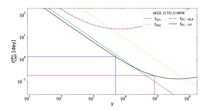
In addition to variability of a specific band, the measurement of time delays between variations in different energy bands can also provide an important limit to the possible values of the physical parameters in the framework of the one-zone leptonic model. A natural way to explain these lags is to interpret them as the cooling time difference of the relativistic electrons (e.g., Takahashi et al., 1996). In Fig. 7, we plot the cooling timescales of different radiation processes in the observers’ frame as a function of for 4FGL J1751.5+0938 (under the parameter set as shown in Table 2). Since the emissions of 0.1-1 GeV and 1-300 GeV (for simplicity, we take the average values of these ranges for analysis) usually mainly come from the EC-DT (DT is the main photon field), the corresponding electron Lorentz factors can be estimated by using the monochromatic approximation as
| (26) |
where is the peak frequency of the DT radiation. The obtained electron Lorentz factors and the corresponding EC-DT cooling timescales are marked with blue and red curves in Fig. 7, respectively. It can be seen that the flare in 0.1-1 GeV lags behind the flare in 1-300 GeV, and the KN effect can be neglected, then the time lag can be given by
| (27) |
Substituting Eq. (26) into Eq. (27), can be derived as
| (28) |
Combining Eq. (16) and given by the reverberation mapping, we have . If assuming that the dissipation occurs within the DT (then can be approximated as a constant), and can be collected, we can obtain the value of . If it is consistent with the lower limit of obtained from the internal absorption (e.g., Dondi & Ghisellini, 1995), we suggest that the location of the emitting region should be inside the DT, and there should be strong EC-DT radiation in the high-energy peak, otherwise we suggest that the emitting region should be outside the DT, resulting in a smaller value of , and thus obtaining a larger value of to achieve consistency. Using Eq. (28), we have
| (29) |
It can be seen that if is determined, will become a constant. Since the rough ratio of can be obtained from the quasi-simultaneous multi-wavelength SED of 4FGL J1751.5+0938 (see Fig. 2), where and are the total luminosities of the dominant EC and SSC emissions, respectively. Combining with derived from the time delay, we can obtain the values of , , and successively. More specifically, we can get the value of from . Then, by combining with the causality relation, we can estimate the value of from . Finally, we can infer from , and then determine the origin of the high-energy peak. On the other hand, as discussed in Section 4.1 and shown in Fig. 7, if the soft photons mainly originate from the BLR, the cooling efficiency of the electrons producing 150 GeV emission would be greatly reduced due to the severe KN effect, and it may result in a cooling time similar to that of the electrons producing 500 MeV emission. Therefore, for a specific source, if a reliable time delay between the 500 MeV and 150 GeV emissions cannot be found, we suggest that its EC process should be dominated by EC-BLR, and then the emitting region might be located inside or outside but very close to the BLR. Similar to the time delay between MeV and GeV, the time lag between flares in the infrared bands and the GeV can also help constrain the parameters. The difference is that the Lorentz factors of the electrons producing the infrared emission is much lower than that producing the GeV emission, resulting in the observed time lag being basically equal to the cooling time of the electrons’ synchrotron radiation (see Fig. 7). Then, we have . It can be seen that if can be determined, the value of can be obtained. On the other hand, we can get the value of from corresponding to the infrared emission. If we fix the Doppler factor to 11.7, the corresponding magnetic field and electron Lorentz factor can be estimated (e.g., Takahashi et al., 1996). Therefore, we believe that the variability timescale is very helpful for the study of blazars.
5 Conclusion
We propose an analytical method to assess the necessity of external photon fields for LBLs in the framework of one-zone scenario. Based on obtained analytical results, we fit the quasi-simultaneous multi-wavelength SEDs of 15 -4LAC LBLs with the conventional one-zone leptonic model to investigate the physical properties of -4LAC LBLs. Our main results are summarized below. (1) We find that most of the LBLs’ SEDs cannot be fitted by the one-zone SSC model, which implies that the introduction of external photon fields is almost inevitable for the explanation of the high-energy peak. Therefore, our results indicate that LBLs are masquerading BL Lacs, confirming the difference in physical properties between LBLs and IBLs/HBLs (e.g., Yan et al., 2014; Fan et al., 2012). (2) We suggest that the -ray emitting regions of LBLs are located outside the BLR and within the DT. (3) By extending the analytical method to all types of LSPs in -4LAC (using archival data; Yang et al., 2022, 2023), we find that the high-energy peaks of some FSRQs and BCUs can be explained by the SSC emission, implying that the importance of external photons could be minor. (4) Our results suggest that the variability timescale may be a useful indicator to the origin of the high-energy peak, and the high-energy peak is only possible to originate from the SSC emission in the case of relatively long variability timescale.
Acknowledgements
This work is partially supported by the National Key Research and Development Program of China (grant numbers 2022SKA0130100 and 2022SKA0130102). R.X. acknowledges the support by the NSFC under Grant No. 12203043. F.K.P acknowledges support by the National Natural Science Foundation of China (Grants No. 12003002), the University Annual Scientific Research Plan of Anhui Province 2023 (2023AH050146), the Excellent Teacher Training Program of Anhui Province (2023), and the Doctoral Starting up Foundation of Anhui Normal University 2020 (903/752022). Part of this work is based on archival data, software, or online services provided by the SPACE SCIENCE DATA CENTER (SSDC).
Data Availability
The data underlying this article will be shared on reasonable request to the corresponding author.
References
- Abdo et al. (2010a) Abdo A. A., et al., 2010a, ApJ, 712, 957
- Abdo et al. (2010b) Abdo A. A., et al., 2010b, ApJ, 716, 30
- Abdollahi et al. (2022) Abdollahi S., et al., 2022, ApJS, 260, 53
- Ackermann et al. (2011) Ackermann M., et al., 2011, ApJ, 743, 171
- Agudo et al. (2011) Agudo I., et al., 2011, ApJ, 726, L13
- Agudo et al. (2012) Agudo I., et al., 2012, in Journal of Physics Conference Series. p. 012032 (arXiv:1108.0925), doi:10.1088/1742-6596/355/1/012032
- Ajello et al. (2022) Ajello M., et al., 2022, ApJS, 263, 24
- Arsioli & Chang (2018) Arsioli B., Chang Y. L., 2018, A&A, 616, A63
- Atwood et al. (2009) Atwood W. B., et al., 2009, ApJ, 697, 1071
- Bennett et al. (2014) Bennett C. L., Larson D., Weiland J. L., Hinshaw G., 2014, ApJ, 794, 135
- Błażejowski et al. (2000) Błażejowski M., Sikora M., Moderski R., Madejski G. M., 2000, ApJ, 545, 107
- Bloom & Marscher (1996) Bloom S. D., Marscher A. P., 1996, ApJ, 461, 657
- Böttcher (2007) Böttcher M., 2007, Ap&SS, 309, 95
- Böttcher (2019) Böttcher M., 2019, Galaxies, 7, 20
- Böttcher & Bloom (2000) Böttcher M., Bloom S. D., 2000, AJ, 119, 469
- Böttcher & Chiang (2002) Böttcher M., Chiang J., 2002, ApJ, 581, 127
- Böttcher & Els (2016) Böttcher M., Els P., 2016, ApJ, 821, 102
- Brown (2013) Brown A. M., 2013, MNRAS, 431, 824
- Cao & Wang (2013) Cao G., Wang J.-C., 2013, MNRAS, 436, 2170
- Cerruti (2020) Cerruti M., 2020, Galaxies, 8, 72
- Chen (2017) Chen L., 2017, ApJ, 842, 129
- Chen (2018) Chen L., 2018, ApJS, 235, 39
- Chen & Bai (2011) Chen L., Bai J. M., 2011, ApJ, 735, 108
- Chiaberge & Ghisellini (1999) Chiaberge M., Ghisellini G., 1999, MNRAS, 306, 551
- Cleary et al. (2007) Cleary K., Lawrence C. R., Marshall J. A., Hao L., Meier D., 2007, ApJ, 660, 117
- Costamante et al. (2018) Costamante L., Cutini S., Tosti G., Antolini E., Tramacere A., 2018, MNRAS, 477, 4749
- Crusius & Schlickeiser (1986) Crusius A., Schlickeiser R., 1986, A&A, 164, L16
- D’Ammando et al. (2016) D’Ammando F., et al., 2016, MNRAS, 463, 4469
- Deng & Jiang (2023) Deng J., Jiang Y., 2023, MNRAS, 521, 6210
- Deng et al. (2021) Deng X.-J., Xue R., Wang Z.-R., Xi S.-Q., Xiao H.-B., Du L.-M., Xie Z.-H., 2021, MNRAS, 506, 5764
- Dermer (1995) Dermer C. D., 1995, ApJ, 446, L63
- Dermer & Menon (2009) Dermer C. D., Menon G., 2009, High Energy Radiation from Black Holes: Gamma Rays, Cosmic Rays, and Neutrinos
- Dermer & Schlickeiser (1993) Dermer C. D., Schlickeiser R., 1993, ApJ, 416, 458
- Dermer & Schlickeiser (2002) Dermer C. D., Schlickeiser R., 2002, ApJ, 575, 667
- Dermer et al. (2009) Dermer C. D., Finke J. D., Krug H., Böttcher M., 2009, ApJ, 692, 32
- Dermer et al. (2012) Dermer C. D., Murase K., Takami H., 2012, ApJ, 755, 147
- Dimitrakoudis et al. (2012) Dimitrakoudis S., Mastichiadis A., Protheroe R. J., Reimer A., 2012, A&A, 546, A120
- Ding et al. (2017) Ding N., Zhang X., Xiong D. R., Zhang H. J., 2017, MNRAS, 464, 599
- Dondi & Ghisellini (1995) Dondi L., Ghisellini G., 1995, MNRAS, 273, 583
- Dotson et al. (2012) Dotson A., Georganopoulos M., Kazanas D., Perlman E. S., 2012, ApJ, 758, L15
- Fan et al. (2006) Fan Z., Cao X., Gu M., 2006, ApJ, 646, 8
- Fan et al. (2012) Fan J. H., Yang J. H., Yuan Y. H., Wang J., Gao Y., 2012, ApJ, 761, 125
- Fossati et al. (1998) Fossati G., Maraschi L., Celotti A., Comastri A., Ghisellini G., 1998, MNRAS, 299, 433
- Frank et al. (2002) Frank J., King A., Raine D. J., 2002, Accretion Power in Astrophysics: Third Edition
- Georganopoulos et al. (2012) Georganopoulos M., Meyer E. T., Fossati G., 2012, arXiv e-prints, p. arXiv:1202.6193
- Ghisellini & Tavecchio (2008) Ghisellini G., Tavecchio F., 2008, MNRAS, 387, 1669
- Ghisellini & Tavecchio (2009) Ghisellini G., Tavecchio F., 2009, MNRAS, 397, 985
- Ghisellini & Tavecchio (2010) Ghisellini G., Tavecchio F., 2010, MNRAS, 409, L79
- Ghisellini et al. (1988) Ghisellini G., Guilbert P. W., Svensson R., 1988, ApJ, 334, L5
- Ghisellini et al. (2005) Ghisellini G., Tavecchio F., Chiaberge M., 2005, A&A, 432, 401
- Ghisellini et al. (2010) Ghisellini G., Tavecchio F., Foschini L., Ghirlanda G., Maraschi L., Celotti A., 2010, MNRAS, 402, 497
- Ghisellini et al. (2014) Ghisellini G., Tavecchio F., Maraschi L., Celotti A., Sbarrato T., 2014, Nature, 515, 376
- Ghisellini et al. (2017) Ghisellini G., Righi C., Costamante L., Tavecchio F., 2017, MNRAS, 469, 255
- Giommi et al. (2012) Giommi P., Padovani P., Polenta G., Turriziani S., D’Elia V., Piranomonte S., 2012, MNRAS, 420, 2899
- Giommi et al. (2013) Giommi P., Padovani P., Polenta G., 2013, MNRAS, 431, 1914
- Grandi et al. (2012) Grandi P., Torresi E., Stanghellini C., 2012, ApJ, 751, L3
- Hayashida et al. (2012) Hayashida M., et al., 2012, ApJ, 754, 114
- Hodgson et al. (2017) Hodgson J. A., et al., 2017, A&A, 597, A80
- Hovatta et al. (2009) Hovatta T., Valtaoja E., Tornikoski M., Lähteenmäki A., 2009, A&A, 494, 527
- Hu et al. (2023) Hu W., Yan D.-H., Hu Q.-L., 2023, ApJ, 948, 82
- Jones (1968) Jones F. C., 1968, Physical Review, 167, 1159
- Jorstad et al. (2010) Jorstad S. G., et al., 2010, ApJ, 715, 362
- Kang et al. (2021) Kang S., et al., 2021, A&A, 651, A74
- Karamanavis et al. (2016) Karamanavis V., et al., 2016, A&A, 590, A48
- Kataoka et al. (1999) Kataoka J., et al., 1999, ApJ, 514, 138
- Katarzyński et al. (2001) Katarzyński K., Sol H., Kus A., 2001, A&A, 367, 809
- Kim et al. (2022) Kim S.-H., et al., 2022, MNRAS, 510, 815
- Li & Kusunose (2000) Li H., Kusunose M., 2000, ApJ, 536, 729
- Li et al. (2022) Li W.-J., Xue R., Long G.-B., Wang Z.-R., Nagataki S., Yan D.-H., Wang J.-C., 2022, A&A, 659, A184
- Liu et al. (2011) Liu H. T., Bai J. M., Wang J. M., Li S. K., 2011, MNRAS, 418, 90
- Liu et al. (2019) Liu R.-Y., Wang K., Xue R., Taylor A. M., Wang X.-Y., Li Z., Yan H., 2019, Phys. Rev. D, 99, 063008
- Madejski & Sikora (2016) Madejski G. G., Sikora M., 2016, ARA&A, 54, 725
- Mankuzhiyil et al. (2011) Mankuzhiyil N., Ansoldi S., Persic M., Tavecchio F., 2011, ApJ, 733, 14
- Mankuzhiyil et al. (2012) Mankuzhiyil N., Ansoldi S., Persic M., Rivers E., Rothschild R., Tavecchio F., 2012, ApJ, 753, 154
- Mannheim (1993) Mannheim K., 1993, A&A, 269, 67
- Massaro et al. (2004) Massaro E., Perri M., Giommi P., Nesci R., 2004, A&A, 413, 489
- Meyer et al. (2011) Meyer E. T., Fossati G., Georganopoulos M., Lister M. L., 2011, ApJ, 740, 98
- Nalewajko et al. (2014) Nalewajko K., Begelman M. C., Sikora M., 2014, ApJ, 789, 161
- O’Sullivan & Gabuzda (2009) O’Sullivan S. P., Gabuzda D. C., 2009, MNRAS, 400, 26
- Padovani et al. (2019) Padovani P., Oikonomou F., Petropoulou M., Giommi P., Resconi E., 2019, MNRAS, 484, L104
- Paliya et al. (2017) Paliya V. S., Marcotulli L., Ajello M., Joshi M., Sahayanathan S., Rao A. R., Hartmann D., 2017, ApJ, 851, 33
- Pushkarev et al. (2012) Pushkarev A. B., Hovatta T., Kovalev Y. Y., Lister M. L., Lobanov A. P., Savolainen T., Zensus J. A., 2012, A&A, 545, A113
- Ramakrishnan et al. (2015) Ramakrishnan V., Hovatta T., Nieppola E., Tornikoski M., Lähteenmäki A., Valtaoja E., 2015, MNRAS, 452, 1280
- Rieger et al. (2007) Rieger F. M., Bosch-Ramon V., Duffy P., 2007, Ap&SS, 309, 119
- Rybicki & Lightman (1979a) Rybicki G. B., Lightman A. P., 1979a, Radiative processes in astrophysics
- Rybicki & Lightman (1979b) Rybicki G. B., Lightman A. P., 1979b, Astronomy Quarterly, 3, 199
- Sahakyan & Giommi (2021) Sahakyan N., Giommi P., 2021, MNRAS, 502, 836
- Saldana-Lopez et al. (2021) Saldana-Lopez A., Domínguez A., Pérez-González P. G., Finke J., Ajello M., Primack J. R., Paliya V. S., Desai A., 2021, MNRAS, 507, 5144
- Schlickeiser & Ruppel (2010) Schlickeiser R., Ruppel J., 2010, New Journal of Physics, 12, 033044
- Shakura & Sunyaev (1973) Shakura N. I., Sunyaev R. A., 1973, A&A, 24, 337
- Sikora et al. (1994) Sikora M., Begelman M. C., Rees M. J., 1994, ApJ, 421, 153
- Sikora et al. (2009) Sikora M., Stawarz Ł., Moderski R., Nalewajko K., Madejski G. M., 2009, ApJ, 704, 38
- Sokolov & Marscher (2005) Sokolov A., Marscher A. P., 2005, ApJ, 629, 52
- Stratta et al. (2011) Stratta G., Capalbi M., Giommi P., Primavera R., Cutini S., Gasparrini D., 2011, arXiv e-prints, p. arXiv:1103.0749
- Takahashi et al. (1996) Takahashi T., et al., 1996, The Astrophysical Journal, 470, L89
- Tan et al. (2020) Tan C., Xue R., Du L.-M., Xi S.-Q., Wang Z.-R., Xie Z.-H., 2020, ApJS, 248, 27
- Tavecchio & Ghisellini (2008) Tavecchio F., Ghisellini G., 2008, MNRAS, 386, 945
- Tavecchio et al. (1998) Tavecchio F., Maraschi L., Ghisellini G., 1998, ApJ, 509, 608
- Tavecchio et al. (2010) Tavecchio F., Ghisellini G., Bonnoli G., Ghirlanda G., 2010, MNRAS, 405, L94
- Tramacere et al. (2011) Tramacere A., Massaro E., Taylor A. M., 2011, ApJ, 739, 66
- Urry & Padovani (1995) Urry C. M., Padovani P., 1995, PASP, 107, 803
- Vovk & Neronov (2013) Vovk I., Neronov A., 2013, ApJ, 767, 103
- Wang & Xue (2021) Wang Z.-R., Xue R., 2021, Research in Astronomy and Astrophysics, 21, 305
- Wang et al. (2023) Wang Z.-R., Xue R., Xiong D., Wang H.-Q., Sun L.-M., Peng F.-K., 2023, arXiv e-prints, p. arXiv:2308.10200
- Xiao et al. (2022a) Xiao H., Ouyang Z., Zhang L., Fu L., Zhang S., Zeng X., Fan J., 2022a, ApJ, 925, 40
- Xiao et al. (2022b) Xiao H., Fan J., Ouyang Z., Hu L., Chen G., Fu L., Zhang S., 2022b, ApJ, 936, 146
- Xue et al. (2019) Xue R., Liu R.-Y., Petropoulou M., Oikonomou F., Wang Z.-R., Wang K., Wang X.-Y., 2019, ApJ, 886, 23
- Xue et al. (2022) Xue R., Wang Z.-R., Li W.-J., 2022, Phys. Rev. D, 106, 103021
- Xue et al. (2023) Xue R., Huang S.-T., Xiao H.-B., Wang Z.-R., 2023, Phys. Rev. D, 107, 103019
- Yan et al. (2012) Yan D., Zeng H., Zhang L., 2012, MNRAS, 424, 2173
- Yan et al. (2014) Yan D., Zeng H., Zhang L., 2014, MNRAS, 439, 2933
- Yan et al. (2018) Yan D., Wu Q., Fan X., Wang J., Zhang L., 2018, ApJ, 859, 168
- Yang et al. (2022) Yang J. H., et al., 2022, ApJS, 262, 18
- Yang et al. (2023) Yang J., et al., 2023, Science China Physics, Mechanics, and Astronomy, 66, 249511
- Zdziarski et al. (2012) Zdziarski A. A., Sikora M., Dubus G., Yuan F., Cerutti B., Ogorzałek A., 2012, MNRAS, 421, 2956
- Zhang et al. (2012) Zhang J., Liang E.-W., Zhang S.-N., Bai J. M., 2012, ApJ, 752, 157
- Zhang et al. (2014) Zhang J., Sun X.-N., Liang E.-W., Lu R.-J., Lu Y., Zhang S.-N., 2014, ApJ, 788, 104