Catalytic enhancement in the performance of the microscopic two-stroke heat engine

Abstract

We consider a model of a heat engine operating in the microscopic regime: the two-stroke engine. It produces work and exchanges heat in two discrete strokes that are separated in time. The engine consists of two $d$-level systems initialized in thermal states at two distinct temperatures. Additionally, an auxiliary non-equilibrium system called catalyst may be incorporated into the engine, provided the state of the catalyst remains unchanged after the completion of a thermodynamic cycle. This ensures that the work produced arises solely from the temperature difference, Upon establishing the rigorous thermodynamic framework, we characterize two-fold improvement stemming from the inclusion of a catalyst. Firstly, we show that the presence of a catalyst allows for surpassing the optimal efficiency of two-stroke heat engines which are not assisted by a catalyst. In particular, we prove that the optimal efficiency for two-stroke heat engine consisting of two-level systems is given by the Otto efficiency, and that it can be surpassed via incorporating a catalyst. Secondly, we show that incorporating a catalyst allows the engine to operate in frequency and temperature regimes that are not accessible for non-catalytic two-stroke engines.

I Introduction

In a thermodynamic framework, the role of a catalyst has been addressed at length in studying state interconversion under unitary and Gibbs-preserving transformation [1, 2, 3]. Later, state interconversion with the aid of a catalyst has been generalized to different domains within quantum information theory (see [4, 5] and the references therein). Rather than focusing on the generic state-interconversion in a thermodynamic scenario, we shall address the impact of catalysis on the performance of thermal machines [6, 7, 8]. In particular, we explore how catalysis can lead to the enhancement of efficiency of a microscopic heat engine. A crucial distinction emerges here when comparing the size requirements of catalysts for a generic state interconversion with those for catalytic enhancement in the efficiency of microscopic heat engines. Unlike the asymptotically large catalysts which pose substantial experimental challenges and are often necessitated for state interconversion, our investigation reveals that a catalyst of dimension as modest as two can yield catalytic enhancement in the efficiency and extending the range of operation of a thermal machine. This distinction underscores the novel and practical implications of catalysis in microscopic engines or any other thermodynamic device.

Significance of heat engines comes from the pivotal role they play in transforming heat into work in the realm of thermodynamics. Traditionally, the study of heat engines has been rooted in macroscopic systems, described by classical thermodynamics. However, emergence of quantum mechanics has led to significant progress in understanding the foundational aspects of thermodynamics at the microscopic level. This exciting line of research traces back to thermodynamical analysis of functioning of lasers [9, 10, 11] in the 1950s. Since then, there has been a significant interest in exploring the functioning of quantum thermal machines [12, 13, 14, 15, 16, 17, 18, 19, 20, 21, 22, 23] and developing their microscopic thermodynamical frameworks [24, 25, 26, 27, 28, 29]. Advances in techniques of optical traps [30, 31, 32, 33, 34], nitrogen-vacancy centers in diamond [35], nuclear magnetic-resonance [36], atomic [37] and phononic systems [38], as well as single-electron transistors [39, 40] already enable experimental exploration of quantum effects in nano-scale machines.

The catalytic advancement characterized by this work centers around microscopic two-stroke heat engines that start with two $d$-level systems thermalized at two different temperatures [41, 20, 42, 43, 44, 45, 46]. On the top of this setting, we incorporate an auxiliary non-equilibrium system referred to as the catalyst, with cyclic condition imposed on its marginal state. This ensures that energy of the catalyst does not influence the work and heat associated with the thermal machine.

The first stroke involves switching on interactions among the two $d$-level systems and the catalyst, which results in a joint unitary transformation applied on them. The purpose of this stroke is to extract work through exploitation of non-passivity of the initial combined $d$-level systems and the catalyst. Here, non-passivity of a state refers to the existence of at least a pair of non-degenerate energy levels such that the population associated with the level of higher energy is greater [16]. The interaction is switched off after the extraction of work subjected to the condition that marginal state of the catalyst is same with the initial state, but the catalyst can still be correlated with the other components of the engine. We refer this stroke as the work stroke. On the other hand, the second stroke aims to complete the cycle by rethermalizing the $d$-level systems to their respective initial temperatures via interactions with heat baths. The process of rethermalization leads to consumption and dissipation of the heat to the respective heat baths, as well as destroying the correlations between the catalyst and the other components of the engine. We refer to this stroke as the heat stroke. [12, 47, 48, 49].

Construction of two-stroke thermal machines with the clearly separated phases of work and heat extraction enableds us to perform optimization of machine functioning, which remains challenging without such a structure. This is visibly manifested in the open-system approach, where description of a thermal machine can be given rigorously via master equation formalism. The formalism takes into account various parameters like coupling constants and bath spectral densities [50, 51], admitting for simultaneous and continuous work extraction or consumption [12, 52, 53, 15, 19, 54, 55, 48, 12, 47, 48, 49, 51, 56, 43]. Our model bypasses the need for any detailed knowledge of the dynamics of the physical system, admitting for characterization of the role which a catalyst can play in improving performance of thermal machines.

The main problem we want to focus on in this paper is to optimize the performance of the catalyst assisted two stroke thermal machine that is operating as an engine. In particular, our objective is to maximize quantities as efficiency and work production per cycle. The optimization is done over all unitary transformations during the work stroke. This turns out to be highly nontrivial task, even without a catalyst. For instance, efficiency is not convex in the transformations, as both the denominator - the heat transferred to hot bath, as well as the numerator - the work, depend on the transformation. Therefore one cannot restrict to the set of extremal transformations, which leads to large complications. The level of difficulty is raised even more in the case of catalyst, where we need to preserve its state after completion of the cycle.

In this paper, we aim to partially overcome the above difficulties, by working out a general theory of two stroke engines (with or without catalysis) and providing a series of results regarding optimization of the performance of two stroke engines. We will put more emphasis on the efficiency of the two-stroke engines rather than work extraction which has been extensively explored in Ref. [8]. First of all, we show how the second law holds within the framework of two-stroke engine in the presence and absence of the catalyst. We analyse a two-stroke protocol as a general thermal machine that can work as an engine, cooler or heat pump, and we show that efficiency satisfies the standard inequalities in each case. These general considerations allow us to prove that for general two-stroke engine without a catalyst, the optimal transformation during the first stroke that leads to extraction of work is some permutation that exchanges population among different energy levels. Thus to find optimal efficiency without catalyst one needs to optimize over permutations for different frequency and temperature regimes. Optimizing over permutations for a given frequency and temperature regime is still a formidable task, as the size of the problem grows factorially. Yet, it allowed us to show that for the smallest version two-stroke engine without a catalyst which is composed of two two-level systems thermalized at two different temperatures, the Otto efficiency $1-\omega_{c}/\omega_{h}$ is the optimal efficiency (here $\omega_{h},\omega_{c}$ are frequencies of two-level systems interacting with hot, and cold bath, respectively). This, together with the result from the companion paper in Ref. [46] shows that catalysis can enhance efficiency to a large extent, boosting from the Otto efficiency up to $d$-Otto efficiency given by $1-\omega_{c}/(d\omega_{h})$, where $d$ is dimension of catalyst. As expected, the price for high efficiency is lower work production per cycle in general. This phenomenon is analogue of power-efficiency trade-off in continuous engines [57]. Therefore, we propose a family of permutations which we name simple permutations labelled by $n=1,\ldots d$, giving rise to decreasing efficiencies $1-(n\omega_{c})/(d\omega_{h})$, while increasing amounts of work per cycle. Next, we have shown that catalysis can remarkably enhance the frequency and temperatures regime of operation for the two-stroke engine by considering illustrative examples.

Aiming at optimization of efficiency for catalyst assisted two-stroke engine that transforms via simple permutations during th work stroke, the $d$-Otto efficiency is the optimal one. We also make step forward optimizing work per cycle, by providing a linear program, to compute upper bound for work per cycle in catalytic engine. Finally, we ask: Does there always exist a protocol that led to the enhancement of the efficiency of a given two-stroke engine using a catalyst? Here by given two-stroke engine, we mean two systems with given Hamiltonians. We have answered this question partially via identifying certain cases where one can design protocols that always lead to the catalytic enhancement of efficiency.

This paper is structured as follows: In Sec. II we describe the components and functioning of the two-stroke thermal machines. Our focus narrows to the two-stroke thermal machines operating in the heat engine mode. We define the thermodynamic quantities like heat, work and efficiency in Sec. III. In Sec. IV, we characterize a finite set of transformations that have the possibilities to yield optimal efficiency. Consequently, we are able to devise the smallest two-stroke heat engines and calculate their maximum achievable efficiency. Sec. V analyzes the pivotal role of catalysis in enhancing the efficiency of two-stroke heat engines and broadening the operational regime of the two-stroke engine. We optimize efficiency when the initial state of the engine undergoes a simple permutation. In Sec. VI, we provide a closed-form expression for the work produced by the engine when it operates at maximum efficiency and formulate the optimization of this work, in the presence of a catalyst, as a linear program. Finally, we provide insights into specific scenarios where catalytic enhancement of efficiency can be guaranteed.

II Description of the two-stroke thermal machines

The two-stroke thermal machines consist of two $d$-level systems that are in thermal equilibrium with two separate heat baths. The first $d$-level system $(h)$ is referred to as the hot $d$- level system and is described by the Hamiltonian $H_{h}$. It is connected to a heat bath at an inverse temperature $\beta_{h}$. Similarly, the second $d$-level system $(c)$ is known as the cold $d$- level system and is described by Hamiltonian $H_{c}$. It is connected to a heat bath with an inverse temperature $\beta_{c}$, where $\beta_{c}>\beta_{h}$, that justifies their names. Additionally, one can incorporate an auxiliary system $(s)$ described by Hamiltonian $H_{s}$ with the two-stroke thermal machine in such a way that the marginal state of that system is preserved at the end of the transformation i.e.,

$$\Tr_{h,c}(\rho^{i}_{s,h,c})=\Tr_{h,c}(\rho^{f}_{s,h,c}),$$ (1)

where $\rho^{i}_{s,h,c}$ and $\rho^{f}_{s,h,c}$ denotes the initial and final state of the thermal machine, respectively. This guarantees that any work or heat associated with the thermal machine results exclusively from the temperature gradient of the bath. We shall refer this auxiliary system as the catalyst. In contrast to the hot and cold $d$-level systems, which are in thermal equilibrium with their respective baths, the catalyst is not in equilibrium with either of the bath.

We assume that initially there is no correlation among the hot and cold $d$-level system and the catalyst. Thus, we can write the initial state of the thermal machine as

$$\rho^{i}_{s,h,c}=\rho_{s}\otimes\tau_{h}\otimes\tau_{c},$$ (2)

where $\rho_{s}$ is the initial state of the catalyst, $\tau_{h}$ and $\tau_{c}$ denotes the thermal state of hot and cold $d$-level system i.e.,

$$\tau_{h}=\frac{e^{-\beta_{h}H_{h}}}{\Tr(e^{-\beta_{h}H_{h}})}\quad;\quad\tau_{c}=\frac{e^{-\beta_{c}H_{c}}}{\Tr(e^{-\beta_{c}H_{c}})}.$$ (3)

We treat this thermal machine as an isolated system. In the work stroke, the thermal machine operates via switching on an interaction between all of its components, that results a unitary operation $U$ on the catalyst and the hot and cold $d$-level systems. Therefore, the initial state of the thermal machine $\rho^{i}_{s,h,c}$ is related with its final state $\rho^{f}_{s,h,c}$ by the unitary transformation $U$ i.e.,

$$\rho^{f}_{s,h,c}=U\rho^{i}_{s,h,c}U^{\dagger}.$$ (4)

subjected to the condition of the preservability of the catalyst given in Eq. (1). The work stroke is responsible for extraction of the work exploiting the non-passivity of the initial state of thermal machine $\rho^{i}_{s,h,c}$ where non-passivity. Once the extraction of the work is complete, this interaction is switched off. After the implementation of $U$, in the heat stroke both the $d$ level systems rethermalize to their respective bath temperatures. This stroke requires switching on the interaction between these systems and their respective heat baths, which is subsequently switched off once thermalization is achieved. The process of rethermalization leads to change in the energy of the respective baths which can be associated with the transferring and dumping the heat. Having outlined all the essential components required to define the catalyst-assisted two-stroke thermal machine, we now proceed to its formal definition:

Definition 1 (Catalyst assisted two-stroke thermal machine).

The catalyst assisted two-stroke thermal machine is a thermodynamic device that begins in an initial state

$$\rho^{i}_{s,h,c}=\rho_{s}\otimes\tau_{h}\otimes\tau_{c},$$ (5)

and operate in two discrete strokes to accomplish a desired task in the following manner:

1. Work stroke: In this stroke, the interaction among the components of thermal machine is switched on. As a consequence, the initial state of the thermal machine $\rho_{s,h,c}^{i}$ undergoes a transformation governed by the unitary $U$:

   $$\rho^{i}_{s,h,c}\to U\rho^{i}_{s,h,c}U^{\dagger}=\rho^{f}_{s,h,c},$$ (6)

   where $U$ satisfies the preservability of the catalyst given in Eq. (1), i.e.,

   $$\Tr_{h,c}\big{(}U\rho_{s,h,c}^{i}U^{\dagger}\big{)}=\Tr_{h,c}\big{(}\rho_{s,h,c}^{i}\big{)}=\rho_{s}.$$ (7)

2. Heat stroke: In this stroke the interaction among the components is switched off and, the hot and the cold $d$-level system rethermalizes to their initial temperatures via switching on interaction with respective heat baths i.e.,

   $$U\rho^{i}_{s,h,c}U^{\dagger} \to \Tr_{h,c}[U\rho^{i}_{s,h,c}U^{\dagger}]\otimes\tau_{h}\otimes\tau_{c}$$ (8)

   $$= \rho_{s}\otimes\tau_{h}\otimes\tau_{c}=\rho^{i}_{s,h,c}.$$

After the end of the heat stroke the thermal machine returns to its initial state that enables to function the thermal machine in a cyclic manner.

Note that, all unitary may not lead to decrease the average energy of the system. The unitary should be constructed based on the intended task to be achieved using the thermal machines. For instance, to further lower the temperature of the cold $d$-level system, we must apply the unitary transformation $U$ in a way that decreases its average energy. On the other hand, in order to extract work from the system, we should apply the unitary transformation $U$ in a manner that extracts the work exploiting the non-passivity of the combined state of the hot and cold $d$-level system and catalyst. In the former scenario, the thermal machine functions as a cooler, while in the latter, it operates as a heat engine.

The Fig. 1 represents a two-stroke thermal machine operating as an heat engine where the hot, the cold $d$-level system and the catalyst are of dimension two. Note that, a two-stroke thermal engines differs from stroke-based thermal engine considered in Ref. [57, 58, 59, 60]. The latter involves three strokes and a working body undergoing a transformation.

It is also possible to miniaturize the two-stroke thermal machines without the catalyst. Naturally, it can be defined in the same manner as definition 1 without the constraint of preserving the state of the catalyst. We shall refer them as the two-stroke thermal machine without catalyst or non-catalytic two-stroke thermal machine. The smallest two-stroke refrigerator and engine without a catalyst has been considered earlier in the literature [20, 42, 44, 41].

The central goal of this paper is to demonstrate how catalysis can significantly improves the performance of the two-stroke thermal machines functioning as heat engines compared to its non-catalytic counterparts.

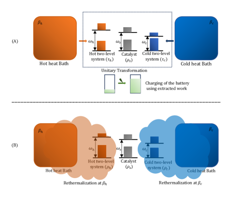
Figure 1: Schematic representation of the smallest two-stroke heat engine with a two-level catalyst: The initial state of the engine consists of hot and cold two-level systems described by Hamiltonian $H_{h}=\omega_{h}|1\rangle\langle 1|$ and $H_{c}=\omega_{c}|1\rangle\langle 1|$, a catalyst with Hamiltonian $H_{s}=\omega|1\rangle\langle 1|$. It starts with two thermalized two-level systems $\tau_{h}$ and $\tau_{c}$ at temperatures $\beta_{h}$ and $\beta_{c}$, along with a two-level catalyst in state $\rho_{s}$. The components are uncorrelated initially. The upper panel (A) depicts the work stroke of the engine where the initial combined state of the components of the engine transforms via a unitary $U$. Our goal is to construct $U$ that leads extraction of work by decreasing the average energy of the initial state subjected to the preservation of the catalyst. The extracted amount of work can be stored via charging a battery (In this paper we will not consider battery explicitly). The lower panel (B) depicts the heat stroke of the engine where the final state of the hot and cold two-level systems $\rho_{h}$ and $\rho_{c}$ rethermalize to their respective initial temperatures which enables the engine to operate in a cyclic manner.

Main Results

Having outlined the functioning of the two-stroke thermal machine, we will now proceed to the main results of this paper. We begin by defining the concepts of heat and work, and describing the first and second law for the catalyst assisted two-stroke heat engine.

III Definition of heat and work

In order to extract or invest work, the two-stroke thermal machine aims to reduce or increase the average energy of the combined state of the hot and cold $d$-level system and the catalyst via the unitary transformation that preserves the marginal state of the catalyst as given in Eq. (7). Therefore, we shall define work as

$$W=\Tr\big((H_{s}+H_{h}+H_{c})(\rho^{i}_{s,h,c}-\rho^{f}_{s,h,c})\big{missing}),$$ (9)

where $\rho^{f}_{s,h,c}=U\rho^{i}_{s,h,c}U^{\dagger}$ is the final state of the thermal machine. In other words, we define work as the change in the energy of the initial state of the thermal machine $\rho^{i}_{s,h,c}$ during the work stroke. This definition is in accordance with classical thermodynamics where work is referred as the change in the energy of a system at constant entropy.

On the other hand, the amount of heat transferred to the thermal machine from the hot heat bath is given by

$$Q_{h}=\Tr\big(H_{h}(\rho^{i}_{s,h,c}-\rho^{f}_{s,h,c})\big{missing})=\Tr(H_{h}(\tau_{h}-\rho_{h})),$$ (10)

where $\rho_{h}$ is the final state of the hot $d$-level system. This definition of heat is also justified based on the traditional perspective of classical thermodynamics, where heat is defined as the amount of energy decreased in the hot heat bath.

Similarly, we also introduce the amount of heat dumped by the thermal machine in the cold bath in a cycle, which is given by

$$Q_{c}=\Tr\big(H_{c}(\rho^{i}_{s,h,c}-\rho^{f}_{s,h,c})\big{missing})=\Tr\big(H_{c}(\tau_{c}-\rho_{c})\big{missing}),$$ (11)

where $\rho_{c}$ denotes the final state of the cold $d$-level system. We refer $Q_{c}$ as cold heat. Using the quantity $Q_{h}$ and $Q_{c}$, one can simplify the definition of work starting from Eq. (9) as follows:

$$W = \Tr\Big((H_{s}+H_{h}+H_{c})(\rho^{i}_{s,h,c}-\rho^{f}_{s,h,c})\Big{missing})$$ (12)

$$= \Tr\Big(H_{h}(\rho^{i}_{s,h,c}-\rho^{f}_{s,h,c})\Big{missing})+\Tr\Big(H_{c}(\rho^{i}_{s,h,c}-\rho^{f}_{s,h,c})\Big{missing})$$

$$= \Tr\big(H_{h}(\tau_{h}-\rho_{h})\big{missing})+\Tr\big(H_{c}(\tau_{c}-\rho_{c}))$$

$$= Q_{h}+Q_{c},$$

where the second equality follows from the fact that the initial state of the catalyst is the same with its final state, as given in Eq. (7). It is worth noting that work associated with the thermal machine given in Eq. (12) is in accordance with the first law.

Since the final marginal state of the catalyst is the same as the initial state, there is no contribution in work $W$ due to the change in the average energy of the catalyst. This can also be seen from Eq. (12) where work associated with the thermal machine depends only on $Q_{h}$ and $Q_{c}$. Thus, without loss of generality, we can assume that the Hamiltonian of the catalyst is trivial. We shall assume the Hamiltonian of the catalyst is trivial for the rest of the paper.

Finally, the efficiency of the thermal machine is calculated by determining the ratio of work and heat i.e.,

$$\eta=\frac{W}{Q_{h}}=1+\frac{Q_{c}}{Q_{h}}.$$ (13)

In this paper, we shall focus mainly on thermal machine that is operating as an engine which aims to produce positive amount of work i.e $W>0$ referred as the two-stroke heat engine. However, thermal machines can also function as coolers or heat pumps. We have provided a comprehensive thermodynamic framework for all modes of two-stroke thermal machines in the appendix A. We have derived the Clausius inequality (a formulation of the second law), which along with Eq. (12) allows us to establish the Carnot bound on efficiency.

In particular, we have shown that a two-stroke thermal machine functioning as an engine if and only if the efficiency $\eta$ is bounded as

$$0<\eta=\frac{W}{Q_{h}}<1-\frac{\beta_{h}}{\beta_{c}}:=\eta_{\text{Carnot}}.$$ (14)

From this point onward, we shall focus on the two-stroke thermal machines operating as engines. To demonstrate the catalytic enhancements in the performance, it is essential to understand what is the optimal performance of the engine without the catalyst. In the next section, we will characterize the transformations that results in achieving the optimal efficiency for a two-stroke engine without a catalyst. As a consequence, we will derive the expression for the optimal efficiency of the smallest two-stroke engine.

IV Two-stroke heat engine without a catalyst

In this section we will aim at optimizing efficiency of the two-stroke engine without catalysis. This is highly nontrivial task, mainly because the efficiency is not a convex function of the protocols. Below we will prove that for two-stroke engines, optimal efficiency is nevertheless obtained by maximizing solely over extreme protocols - which are actually permutations of levels of hot and cold d-level systems. We next apply this result to prove in Sec. IV.2 that for the smallest engine, the Otto efficiency is the maximal attainable one.

IV.1 Optimal performance of the the two-stroke heat engine without catalyst

In this section, we shall characterize the transformations that lead to optimal efficiency for a two-stroke engine without a catalyst.

The two-stroke heat engine starts with the initial state $\tau_{h}\otimes\tau_{c}$ that transforms via a unitary $U$. Recall that $\tau_{h}$ and $\tau_{c}$ denotes the thermal state of the hot and cold $d$-level system defined in Eq. (3). In order to optimize the efficiency, we will show that among all the unitaries $U$ that can act on $\tau_{h}$ and $\tau_{c}$, only permutation could possibly lead to the maximum efficiency and production of work for the two-stroke engine. We shall formalize this in the following theorem:

Theorem 1.

The maximum work extraction and efficiency of a two-stroke heat engine without a catalyst are achieved when the initial state of the hot and cold $d$-level system, $\rho^{i}_{h,c}=\tau_{h}\otimes\tau_{c}$, transforms via a unitary which performs a permutation of energy levels. Moreover, for some range of parameters the maximum work extraction and maximum efficiency are not attainable simultaneously via the same permutation.

As $\rho^{i}_{h,c}$ is diagonal in the total energy eigenbasis and work defined in Eq. (9) is linear, it is simple to see that maximum work will be achieved if the initial state transforms via a permutation which is given by the ergotropy of the initial state [16, 61]. On the other hand optimization of the efficiency is not straightforward. The proof relies on the thermodynamic framework for the two-stroke thermal machine discussed in appendix A and the proof of this theorem is given in appendix B.

This theorem reduces efficiency optimization as a optimization problem over finitely many states, though the number of states increases factorially with size. But, we shall see in the next section that theorem 1 extremely simplifies the calculation of optimal efficiency for the smallest two-stroke heat engine that constitutes of two-level systems only. On the other hand, the optimization of work is much easier for any given initial state $\tau_{h}\otimes\tau_{c}$, because work will be maximized for the permutation that leads to the passive version of the state $\tau_{h}\otimes\tau_{c}$ [16].

IV.2 Optimal performance of the smallest two-stroke heat engine

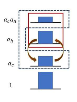
Figure 2: This picture shows the permutation leads to optimal production of work and efficiency for the smallest two-stroke engine without a catalyst. This permutation exchanges the population between the second and the third excited state. This results a net population flow from the subspace where hot two-level system is excited (enclosed in red square) to the subpace where cold two-level system is excited (enclosed by blue dashed lines).

The smallest two-stroke heat engine is constructed with considering $\tau_{h}$ and $\tau_{c}$ as two level systems. The initial state of the hot and cold $d$-level system is given by $\tau_{h}\otimes\tau_{c}$ and the Hamiltonian is $H_{h}+H_{c}$ where

$$\tau_{i} = \frac{1}{1+e^{-\beta_{i}\omega_{i}}}(|0\rangle\langle 0|+e^{-\beta_{i}\omega_{i}}|1\rangle\langle 1|),$$ (15)

$$H_{i} = \omega_{i}|1\rangle\langle 1|,$$ (16)

where $i\in\{h,c\}$ and $\beta_{h}\omega_{h}\leq\beta_{c}\omega_{c},\;\;\omega_{h}>\omega_{c}$. Observe that the smallest two-stroke engine without a catalyst can not extract work if $\omega_{c}>\omega_{h}$ as this makes the state $\tau_{h}\otimes\tau_{c}$ passive.

As we have seen from theorem 1, the optimal efficiency of the engine is achieved for some permutation. In the scenario where $\tau_{h}$ and $\tau_{c}$ are two level system, the only permutation for which the engine can extract positive amount of work is

$$\Pi=(|0,0\rangle\langle 0,0|+|0,1\rangle\langle 1,0|+|1,0\rangle\langle 0,1|+|1,1\rangle\langle 1,1|)_{h,c},$$ (17)

where the first and second index in $|\cdot\rangle\langle\cdot|$ corresponds to the energy levels of the hot and cold $d$-level systems, respectively (See Fig. 2).

The work produced by the engine and the transferred amount of heat is given by

$$W = \mathcal{N}(a_{h}-a_{c})(\omega_{h}-\omega_{c}),,$$ (18)

$$Q_{h} = \mathcal{N}(a_{h}-a_{c})\omega_{h},$$ (19)

where

$$a_{h}:=e^{-\beta_{h}\omega_{h}},\quad a_{c}:=e^{-\beta_{c}\omega_{c}},\quad\mathcal{N}=\frac{1}{(1+a_{h})(1+a_{c})}.$$ (20)

This allows us to compute the optimal efficiency by taking their ratio

$$\eta=1-\frac{\omega_{c}}{\omega_{h}}.$$ (21)

The amount of work produced by the engine also maximized when $\tau_{h}\otimes\tau_{c}$ undergoes transformation via the permutation given Eq (17) as it results to the passive state. Thus, we can infer that work given in Eq. (18) will be the maximum work that can be produced by the engine. This efficiency given in Eq. (21) is referred as the Otto efficiency. Since, the permutation in Eq. (17) leads to the simultaneous maximization of work and efficiency, the work-efficiency trade-off relation becomes trivial.

Furthermore, note that, when $\beta_{h}\omega_{h}=\beta_{c}\omega_{c}$, this engine reaches the Carnot efficiency, whereas work produced by the engine becomes zero. This is in agreement to our understanding of classical thermodynamics that says that the amount of work produced per cycle approaches zero when an engine operates with Carnot efficiency. The detailed calculation can be found in appendix C. In the next section, we shall show that one can surpass this optimal Otto efficiency given in Eq. (21) using a catalyst.

V Catalytic enhancement

In this section, we shall explore the role of catalysis in enhancing the performance of the two-stroke heat engine. Our primary focus will be on the smallest version of the two-stroke heat engine, where the dimensions of the hot and cold $d$-level systems are two, whose optimal efficiency aligns with the Otto efficiency. We shall use the following notation to describe the smallest two-stroke engine

1. $\omega_{h}$ and $\omega_{c}$ to denote the energy of the excited state two-level Hamiltonian $H_{h}$ and $H_{c}$ as described in Eq. (15). Like earlier, we shall assume the energy of the ground state is $0$.

2. $a_{h}$ and $a_{c}$ to denote the Gibbs factor and $\mathcal{N}$ denote the normalization constant i.e.,

   $$\mathcal{N}=\frac{1}{(1+a_{h})(1+a_{c})}$$ (22)

   as introduced in Eq. (20).

The main challenge in optimizing work production and efficiency arises from the variability of the state of the catalyst along with the unitary $U$. This complexity makes the problem hard to solve, even when the catalyst is a two-level system. To tackle this, we will confine ourselves to a specific set of transformations referred to as simple permutations, elaborated in the later section. Our aim is to derive a closed form for the maximum efficiency of a two-stroke engine, with an initial state undergoing transformation through simple permutations.

Before proceeding to the optimization of the efficiency, we shall show that energetic coherence of the state of catalyst can not influence the performance. Hence, it is enough to focus on the energy incoherent catalysts only.

V.1 Coherence in the initial state of the catalyst can not enhance the performance of the two-stroke heat engine

In this section, we shall show that considering the catalyst that are diagonal in its energy eigenbasis are enough for the optimization of the efficiency and the work in the following proposition.

Proposition 2.

For any catalyst assisted two-stroke heat engine starting with initial state $\rho_{s}\otimes\tau_{h}\otimes\tau_{c}$ that produces work $W$ with efficiency $\eta$, one can construct a unitary that transforms the initial state of another two-stroke heat engine that starts in $\tilde{\rho}_{s}\otimes\tau_{h}\otimes\tau_{c}$ such that state of the catalyst $\tilde{\rho}_{s}$ satisfies $[\tilde{\rho}_{s},H_{s}]=0$ and produces exactly same work $W$ with the efficiency $\eta$.

Thanks to proposition 2, from now on we shall only focus on the catalyst that are diagonal. The proof of this theorem is given in appendix D. Now, let us clarify the kinds of catalytic enhancements that we have investigated in this paper in the following section.

V.2 Two kinds of catalytic enhancements

In this paper we have mainly investigated the role of the catalyst for a two stroke heat engine where the dimension of hot and cold $d$-level system is two. We recall from Eq. (15) of Sec. IV.2, the initial state of the hot and cold $d$-level system is given by $\tau_{h}\otimes\tau_{c}$ and the Hamiltonian is $H_{h}+H_{c}$. We have explored two kinds of catalytic enhancements for this two-stroke engines.

V.2.1 Catalytic enhancements in the efficiency

As described in Eq. (14), to produce a positive amount of work by a catalyst assisted two-stroke engine its efficiency $\eta$ should satisfy

$$0<\eta<1-\frac{\beta_{h}}{\beta_{c}}.$$ (23)

On the other hand, a two-stroke engine without a catalyst requires to have $\omega_{h}>\omega_{c}$ and $\beta_{h}\omega_{h}>\beta_{c}\omega_{c}$ to produce a positive amount of work, and we have proved that the optimal efficiency is given by the Otto efficiency, i.e., $1-\frac{\omega_{c}}{\omega_{h}}$ (see Sec. IV.2). Therefore, to prove the catalytic enhancement of the efficiency, we aim to achieve an efficiency $\eta$ for the catalyst assisted two-stroke thermal machine such that

$$1-\frac{\omega_{c}}{\omega_{h}}<\eta<1-\frac{\beta_{h}}{\beta_{c}}.$$ (24)

In other words, we shall include a catalyst and construct a unitary that transforms the initial state of the catalyst assisted two-stroke engine such that the above inequality holds.

V.2.2 Extending the regime of operation due to catalysis

The smallest two-stroke heat engine without a catalyst can not extract work if $\omega_{c}>\omega_{h}$, because by definition $\beta_{c}>\beta_{h}$, which implies

$$\omega_{c}>\omega_{h}\Rightarrow e^{-\beta_{h}\omega_{h}}>e^{-\beta_{c}\omega_{c}},$$ (25)

hence making the initial state to be passive [16]. Thus one can not extract any work by applying unitary transformation on such an initial state. Nonetheless, with the aid of a catalyst, we can run the engine at this regime of frequency to extract positive amount of work and run with efficiency $\eta$ that satisfies the inequality in Eq. (23). So, the catalysis can broaden the regime of operations for the two-stroke engine.

V.3 Improving the efficiency using a catalyst

V.3.1 Optimal efficiency of the catalyst-assisted smallest two-stroke heat engine for simple permutation

As mentioned earlier, optimization of efficiency is a formidable task when the initial state of the two-stroke thermal machine transforms via a general unitary during the work stroke. That is why we are going to focus on a simpler class of unitaries: simple permutation. The main motivation for considering this class of permutations are two-fold: on one hand, they are easy to analyze, and on the other hand, any efficiency $\eta$ that satisfy Eq. (23) can be approximated up to an arbitrary precision via a simple permutation by suitably choosing the dimension of the catalyst. In this section, we optimize the efficiency of the smallest two-stroke heat engine assisted with a $d$-level catalyst that undergoes a transformation via a simple permutation. We define simple permutation as follows:

Definition 2 (Simple permutation).

Consider a permutation that acts on $\rho^{i}_{s,h,c}=\rho_{s}\otimes\tau_{h}\otimes\tau_{c}$ with dimension of each component is $d$, $d_{h}$, and $d_{c}$, respectively. We denote the energy eigenstate of total Hamiltonian $H_{s}+H_{h}+H_{c}$ by $|i,j,k\rangle_{s,h,c}$. A permutation $\Pi$ is referred to as a simple permutation, if for any fixed $i$, $\Pi$ acts on exactly two distinct energy levels labelled by $|i,j_{1},k_{1}\rangle$ and $|i,j_{2},k_{2}\rangle$, that exchanges

1. the population between $|i,j_{1},k_{1}\rangle$ with $|i+1,j^{\prime},k^{\prime}\rangle$ and,

2. the population between $|i,j_{2},k_{2}\rangle$ with $|i-1,j^{\prime\prime},k^{\prime\prime}\rangle$,

where $\pm$ involves in $i+1$ and $i-1$, denotes addition or subtraction modulo $d$.

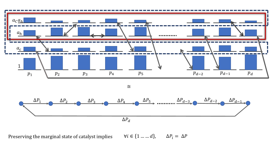
Figure 3: A simple permutation: The above panel depicts a simple permutation with arrows that denotes the exchange the populations among the associated levels. We denote the population associated with energy levels $|i,0,0\rangle_{s,h,c}$, $|i,0,1\rangle_{s,h,c}$, $|i,1,0\rangle_{s,h,c}$, and $|i,1,1\rangle_{s,h,c}$ by $\frac{p_{i}}{(1+a_{c})(1+a_{h})}$, $\frac{p_{i}a_{c}}{(1+a_{c})(1+a_{h})}$, $\frac{p_{i}a_{h}}{(1+a_{c})(1+a_{h})}$, and $\frac{p_{i}a_{c}a_{h}}{(1+a_{c})(1+a_{h})}$, respectively. The enclosed subspace by the red rectangle denotes the hot subspace (taking the sum over all the population enclosed inside the red rectangle gives the population of the excited level of the hot qubit). Similarly, the enclosed subspace by the blue dashed line denotes the cold subspace (taking the sum over all the population enclosed by the blue dashed line rectangle gives the population of the excited level of the cold qubit). The below panel depicts the four energy levels for a fixed $i$ by a blue vertex. The net flow of population from $i^{\text{th}}$ vertex to $(i+1)^{\text{th}}$ is denoted by $\Delta P_{i}$. In order to preserve the marginal state of the catalyst as per Eq. (7), $\forall j$ it requires to satisfy $\Delta P_{j}=\Delta P$

To understand the definition more clearly, see Fig. 3 which shows an example of a simple permutation where $\tau_{h}$ and $\tau_{c}$ are modeled with a qubit. A simple permutation is such a permutation that can be represented by the closed cyclic graph as shown in Fig. 3 with exactly one edge between two vertices. Each vertex corresponds to the population in a particular energy level of the catalyst. The arrow that connects two vertices represents the net flow of the population among the connected vertices and the direction of the arrow gives the direction of the flow of population. For example, in the Fig. 3, $\mathcal{N}p_{1}a_{h}$ flows from vertex $1$ to vertex $2$ and $\mathcal{N}p_{2}a_{c}$ flows from vertex $2$ to vertex $1$. Thus a net population flow of $\Delta P_{1}=\mathcal{N}(p_{1}a_{h}-p_{2}a_{c})$ is created from vertex $1$ to $2$. Importantly, since the marginal state of the catalyst after the permutation has to be the same as its initial state, the net population flow inside a particular vertex has to be the same as the population flows out of that vertex. This implies the following condition:

$$\Delta P_{1}=\Delta P_{2}=\ldots=\Delta P_{d-1}=\Delta P_{d}=\Delta P.$$ (26)

Conceptually, this is similar to Kirchoff’s current law which says the current flowing into a node (or a junction) must be equal to the current flowing out of it which is a consequence of charge conservation. Furthermore, since work done by the engine given in Eq. (12), and the efficiency given in Eq. (13) depends only on the transferred amount of heat $Q_{h}$ and cold heat $Q_{c}$, thus population flow that causes alteration of $Q_{h}$ and $Q_{c}$ will be important to analyze the performance of the engine. To formally characterize the population flow that causes alteration of $Q_{h}$ and $Q_{c}$, we introduce the concepts of hot and cold subspace.

Definition 3 (Hot and cold subspace).

Consider the two-stroke engines whose initial state is given by $\rho^{i}_{s,h,c}$ and the Hamiltonian $H_{s}+H_{h}+H_{c}$ where the dimension of each component is $d$, $d_{h}$, and $d_{c}$, respectively. We denote the energy levels of the Hamiltonian $H_{s}+H_{h}+H_{c}$ by $|i,j,k\rangle_{s,h,c}$. We shall define the $j^{\text{th}}$ hot subspace by

$$\mathcal{H}_{j}:=\text{Span}\;\;\{\forall i,k\;\;|i,j,k\rangle_{s,h,c}\},$$ (27)

and $k^{\text{th}}$ cold subspace by

$$\mathcal{C}_{k}:=\text{Span}\;\;\{\forall i,j\;\;|i,j,k\rangle_{s,h,c}\}.$$ (28)

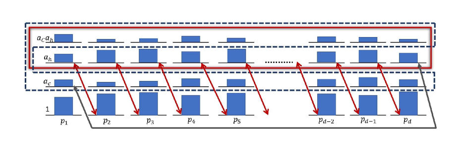
Figure 4: Depiction of the simple permutation described in Eq. (36) that leads to efficiency $\eta=1-\frac{\omega_{c}}{d\omega_{h}}$.

In Fig. 3, the excited hot and cold subspace for a two-stroke heat engine are shown by an enclosed red rectangle and a dotted blue line. Using the idea of the hot and the cold subspace one can simply express the transferred amount of heat $Q_{h}$ given in Eq. (10), by summing the population flow out of the $j^{\text{th}}$ hot subspace multiplied by the corresponding energy of $j^{\text{th}}$ hot subspace i.e.,

$$Q_{h}=\sum_{j}\Delta P_{j}\omega_{h}^{j}.$$ (29)

Similarly, the cold heat $Q_{c}$ given in Eq. (11) reduces by summing the population flow out the $k^{\text{th}}$ cold subspace multiplied by the corresponding energy of $k^{\text{th}}$ cold subspace i.e.,

$$Q_{c}=\sum_{k}\Delta P_{k}\omega_{c}^{k}.$$ (30)

We shall see that Eq. (29) and Eq. (30) simplifies a lot the calculation of efficiency for the simple permutations due the cyclic structure.

Now we shall proceed to optimize the efficiency for the smallest two-stroke heat engines when $\tau_{h}$ and $\tau_{c}$ are of dimension two and assisted with $d$-level catalyst, which is transformed via a simple permutation. In the following theorem, we shall describe this result.

Theorem 3.

Consider the two-stroke heat engines whose initial state is given by $\rho^{i}_{s,h,c}=\rho_{s}\otimes\tau_{h}\otimes\tau_{c}$ with dimension of $\tau_{h}$ and $\tau_{c}$ is two. The initial state of the engine $\rho^{i}_{s,h,c}$ transforms via a simple permutation, where the Hamiltonians and the states of the components are

$$H_{s} = 0\quad;\quad\rho_{s}=\sum_{j=1}^{d}p_{j}|j\rangle\langle j|,$$ (31)

$$H_{h} = \omega_{h}|1\rangle\langle 1|\quad;\quad\tau_{h}=\frac{e^{-\beta_{h}H_{h}}}{\Tr(e^{-\beta_{h}H_{h}})},$$ (32)

$$H_{c} = \omega_{c}|1\rangle\langle 1|\quad;\quad\tau_{c}=\frac{e^{-\beta_{c}H_{c}}}{\Tr(e^{-\beta_{c}H_{c}})},$$ (33)

such that

$$\frac{\omega_{c}}{\omega_{h}}\leq 1\quad\text{and}\quad d\leq\frac{\beta_{c}\omega_{c}}{\beta_{h}\omega_{h}}.$$ (34)

Then the optimal efficiency of such an engine is given by

$$\eta_{\text{opt}}=1-\frac{\omega_{c}}{d\omega_{h}},$$ (35)

where $d$ is the dimension of the catalyst.

Proof sketch.

We shall proceed with achievability of the efficiency $\eta_{\text{opt}}$. In order to prove this, we shall simply consider a permutation [46]:

$$\Pi=(\sum_{i=1}^{d-1}|i,1,0\rangle\langle i+1,0,0|+|1,0,1\rangle\langle d,1,0|)_{s,h,c}$$ (36)

as shown in Fig. 4 which leads to the efficiency of $1-\frac{\omega_{c}}{d\omega_{h}}$. The reason can be easily understood from the Fig. 4. Imagine the each $i^{\text{th}}$ level of the catalyst as a vertex like we described while discussing simple permutation (See Fig. 3). Let us assume this permutation $\Pi$ in Eq. (36) causes $\Delta\tilde{P}$ amount of net population flow from a vertex to its right next one (Remember, due to constraint of preserving the marginal state of the catalyst the transferred amount of population is same for each of the vertex). Therefore, $d\Delta\tilde{P}$ amount of net population flow out of the excited hot subspace (represented by the red arrow in the Fig. 4) whereas $\Delta\tilde{P}$ of net population flow in the excited cold subspace (represented by the grey arrow in the Fig. 4). From the definition of transferred amount of heat $Q_{h}$, and cold heat $Q_{c}$ from Eq. (29) and Eq. (30) we can calculate

$$Q_{h}=d\omega_{h}\Delta\tilde{P};\quad Q_{c}=-\omega_{c}\Delta\tilde{P}.$$ (37)

Note that, as the net population flows in the excited cold subspace, to be consistent with Eq. (30) we put a negative sign to calculate $Q_{c}$. Using the formula of efficiency from Eq. (13) we can obtain $\eta=1-\frac{\omega_{c}}{d\omega_{h}}$. The condition $d\leq\frac{\beta_{c}\omega_{c}}{\beta_{h}\omega_{h}}$ given in Eq. (34) ensures that the efficiency given in Eq. (35) is upper bounded by Carnot efficiency. We have presented the complete proof in appendix LABEL:appendix4 where we establish the optimality of the bound.

∎

Here we would like to make a remark. By inspection, we can observe that there is a family of permutations, that leads to the efficiency $1-\frac{\omega_{c}}{d\omega_{h}}$ which is obtained by swapping the position of red arrows and grey arrow in Fig. 4. Because all permutations within this family will lead to $\Delta\tilde{P}$ amount of net population flow in the cold subspace and $d\Delta\tilde{P}$ amount of net population flow out the hot subspace. On the other hand, in order to calculate the amount of work produced by the engine we employ Eq. (12) that results:

$$W=Q_{h}+Q_{c}=(d\omega_{h}-\omega_{c})\Delta\tilde{P}.$$ (38)

To calculate $\Delta\tilde{P}$ one needs apply the condition of preserving the marginal state of the catalyst (cyclicity) which we shall do in the later section.

We now turn our attention to the question: Can we always ensure catalytic improvements in the efficiency of the smallest two-stroke engine? It is worth noting that the permutation in Eq. (36) fails to facilitate work extraction whenever Eq. (34) is not satisfied. Thus, catalytic enhancements in the efficiency is not always ensured via the permutation $\Pi$ Eq. (36). In the next section, we will construct a more general simple permutation than $\Pi$ given in Eq. (36), which always leads to catalytic enhancement in efficiency.

V.3.2 Catalysis always enhances the efficiency of a smallest two-stroke engine

Figure 5: A generic simple permutation described in Eq. (VI.1) that contains the simple permutation showed in Fig. 4 as a special case with $n=1$ and $m=d-1$. This leads to efficiency $\eta=1-\frac{n\omega_{c}}{(m+n)\omega_{h}}$.

In this section, we shall construct a simple permutation that will always allow us to surpass the optimal Otto efficiency of the smallest two-stroke engine. We shall construct a permutation such that the efficiency $\eta$ of the two-stroke thermal machine satisfy inequality in Eq. (24) for any ratio of frequency and temperature. We shall describe the result in the following theorem.

Theorem 4.

Consider a two-stroke heat engine without a catalyst such that the dimension of both the hot and cold $d$-level system is two. Let us assume the energy of the excited state for the hot two-level system is greater than the energy of the excited state for the cold two-level system i.e., $\omega_{h}>\omega_{c}$. Then, it is always possible to incorporate a catalyst and construct a unitary which leads to the efficiency $\eta$ strictly greater than optimal Otto efficiency of the non-catalytic two-stroke engine i.e.,

$$1-\frac{\omega_{c}}{\omega_{h}}<\eta<1-\frac{\beta_{h}}{\beta_{c}}.$$ (39)

Proof.

Consider the simple permutation $\Pi_{\text{gen}}$ given by

$$\Pi_{\text{gen}} = \big{(}\sum_{i=1}^{m}|i+1,0,0\rangle\langle i,1,0|$$

$$+ \sum_{j=m+1}^{m+n-1}|j+1,0,1\rangle\langle j,1,0|$$

$$+ |1,0,1\rangle\langle m+n,1,0|+\text{Herm. conjugate}\big{)}_{s,h,c}\;,$$

where,

$$d=m+n,$$ (41)

as shown in Fig. 5 where dimension of the catalyst. Let us assume that $\Delta P$ is population flow that happens from one vertex to its next one. As mentioned earlier, due to catalysis all the vertex must transfer same amount of population to the next one. Employing the formula from Eq. (29) and Eq. (30), we can calculate

$$Q_{h}=(m+n)\Delta P\omega_{h}=d\Delta P\omega_{h}\quad Q_{c}=-n\Delta P\omega_{c},$$ (42)

where negative sign in $Q_{c}$ implies population flow in the excited cold subspace. Thus, the efficiency can be calculated from Eq. (13) as

$$\eta=1+\frac{Q_{c}}{Q_{h}}=1-\frac{n\omega_{c}}{(m+n)\omega_{h}}=1-\frac{n\omega_{c}}{d\omega_{h}}.$$ (43)

In order to satisfy Eq. (39), it is enough to satisfy the following inequality.

$$\frac{\omega_{c}}{\omega_{h}}<\frac{d}{n}<\frac{\beta_{c}\omega_{c}}{\beta_{h}\omega_{h}}.$$ (44)

It is always possible to choose $d$ and $n$ such that the above inequality holds because $\frac{d}{n}$ is a rational number, thus it can approximate any real number between $\frac{\omega_{c}}{\omega_{h}}$ and $\frac{\beta_{c}\omega_{c}}{\beta_{h}\omega_{h}}$ with arbitrary accuracy. ∎

Here we would like to make a remark about the simple permutation $\Pi_{\text{gen}}$ defined in Eq. (V.3.2). Note that, any possible efficiency that can be achieved by the two-stroke engine must lies in between $0$ and Carnot efficiency as mentioned in Eq. (23). Now any efficiency between $0$ and Carnot efficiency can be realized by choosing $n$ and $d$ in the simple permutation $\Pi_{\text{gen}}$. So, the inclusion of a catalyst of suitably chosen dimension enables to realize any possible value of efficiency of the heat engine, i.e., any $\eta$ that satisfy Eq. (23). We shall elaborate the idea in the next section.

We shall explore now the another kind of catalytic enhancement which is about broadening of the operational regime of the two-stroke heat engine.

V.4 Extending the regime of operations for the two-stroke thermal machine

In this section, we shall explore the second kind of catalytic enhancement. We shall demonstrate that catalyst enables the two-stroke heat engine to extract work in a regime of frequency and temperature where the it is impossible for a non-catalytic two-stroke engine. Let us illustrate the idea via a numerical example for a two-stroke engine where the dimension of the hot and cold $d$-level system is restricted to $2$.

Example: Consider a two-stroke engine where the cold $d$-level system is thermalized at inverse temperature $\beta_{c}=7$ and the hot $d$-level system is thermalized at inverse temperature $\beta_{h}=6$ . We consider the Hamiltonian of the hot and cold $d$-level system as:

$$H_{h} = \omega_{h}|1\rangle\langle 1|,\quad H_{c}=\omega_{c}|1\rangle\langle 1|$$ (45)

$$\quad\text{with}\;\;\omega_{h}=2,\;\omega_{c}=3.$$

Clearly, at this regime of temperature and frequency the two-stroke engine can not produce work since

$$\frac{\omega_{c}}{\omega_{h}}=\frac{3}{2}>1.$$ (46)

which makes the optimal efficiency (Otto efficiency) given in Eq. (21) negative. One can check this also by computing the initial state which turns out to be passive:

$$\tau_{h}\otimes\tau_{c} = \frac{1}{(1+a_{h})(1+a_{c})}(1,\;a_{h},\;a_{c},\;a_{c}a_{h})$$

$$= \frac{1}{(1+e^{-12})(1+e^{-21})}(1,\;e^{-12},\;e^{-21},\;e^{-33})$$

where $a_{h}:=e^{-\beta_{h}\omega_{h}}=e^{-12}$ and $a_{c}:=e^{-\beta_{c}\omega_{c}}=e^{-21}$. The passivity is reflected from the fact that $\omega_{c}>\omega_{h}$ whereas $a_{c}<a_{h}$. So, one can not extract work from such an initial state via unitary operation. Now, we can make this engine to produce positive amount of work with the aid of a catalyst. Note that, we have

$$\frac{\omega_{c}}{\omega_{h}}=\frac{3}{2}<\frac{\beta_{c}\omega_{c}}{\beta_{h}\omega_{h}}=\frac{7}{4},$$ (48)

thus, in order to extract positive amount of work via the simple permutation given in Eq. (V.3.2), we need to choose the dimension of the catalyst $d$ and the parameter $n$ such that Eq. (44) holds. We choose $d=5$ and $n=3$, then clearly

$$\frac{\omega_{c}}{\omega_{h}}=\frac{3}{2}=1.5<\frac{d}{n}=\frac{5}{3}\simeq 1.67<\frac{\beta_{c}\omega_{c}}{\beta_{h}\omega_{h}}=\frac{7}{4}=1.75.$$ (49)

Employing the formula of efficiency from Eq. (43), we can easily calculate the efficiency

$$\eta=1-\frac{3\omega_{c}}{5\omega_{h}}=1-\frac{9}{10}=0.1.$$ (50)

As the efficiency $\eta$ satisfies Eq. (44) (or Eq. (23)), this ensures that engine will produce positive work. One can calculate produced amount of work by the engine via calculating $Q_{h}$ and $Q_{c}$ from Eq. (29) and Eq. (30), respectively.

This example exhibits two very crucial features about the catalyst assisted two-stroke engine that transforms according to the simple permutation $\Pi_{\text{gen}}$. First, if we apply the simple permutation given in Eq. (36) to extract work, it will not be possible because $n=1$ for this permutation, which implies

$$\frac{d}{n}=d.$$ (51)

Therefore, for any value of $d$ the Eq. (44) can not be satisfied. So, in that case we need to suitably choose $d$ and $n$ in a way in the simple permutation Eq. (VI.1) such that Eq. (44) is satisfies. Second, the catalyst enables the engine to produce work in a regime of frequency and temperature, where it is impossible to work for a non-catalytic two-stroke engine. From the second law, we know that in order to extract work the efficiency $\eta$ should satisfy the inequality in Eq. (14) i.e.,

$$0<\eta<1-\frac{\beta_{h}}{\beta_{c}}.$$ (52)

Now, one can choose $n$ and $d$ in the expression of efficiency in Eq. (43), such that the above inequality holds. Or equivalently, one can choose $n$ and $d$ always such that the following holds:

$$0<1-\frac{n\omega_{c}}{d\omega_{h}}<1-\frac{\beta_{h}}{\beta_{c}}\Rightarrow\frac{\omega_{h}}{\omega_{c}}>\frac{n}{d}>\frac{\beta_{h}\omega_{h}}{\beta_{c}\omega_{c}}.$$ (53)

Therefore, it implies that catalyst can enable the two-stroke engine for any ratio of frequency and temperature. We shall summarize the discussion in the following theorem:

Theorem 5.

Consider a catalyst assisted two stroke heat engine where the dimension of the hot and cold $d$-level system is two. It can produce work at any regime of frequency and temperature ratio $\frac{\omega_{h}}{\omega_{c}}$ and $\frac{\beta_{h}}{\beta_{c}}$ for suitably chosen dimension of the catalyst and the value of $n$ in the permutation $\Pi_{\text{gen}}$ defined in Eq. (V.3.2).

In Fig. 6 we have plotted the maximum regime of operation for the two-stroke engine with the dimension of hot and cold $d$-level system is two where we have shown that catalyst of small dimension like $2,\;3,\;4$, significantly enhances the regime of the operation for the two-stroke engine. On top of that, we have observed that catalyst enables the engine to extract work whenever $\frac{\omega_{h}}{\omega_{c}}>\frac{\beta_{h}\omega_{h}}{\beta_{c}\omega_{c}}$.

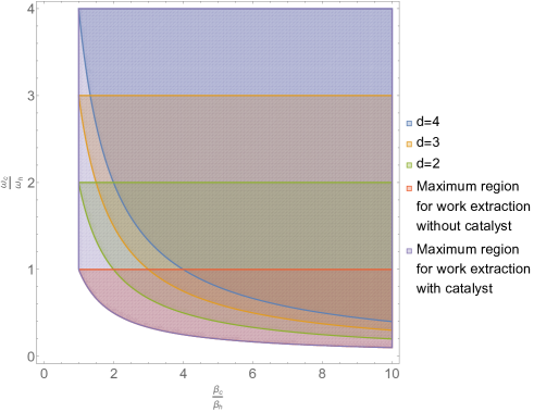
Figure 6: This figure depicts the maximum region where the engine with as well as without catalyst can produce positive amount of work for the range $\frac{\omega_{c}}{\omega_{h}}\in(0,4)$ and $\frac{\beta_{c}}{\beta_{h}}\in(0,10)$. The maximum regime where positive amount of work extraction by the engine is possible whenever $\frac{\omega_{c}}{\omega_{h}}<\frac{\beta_{c}\omega_{c}}{\beta_{h}\omega_{h}}$ is shown in purple. The regime for work extraction via simple permutation given in Eq. (36) for catalyst dimension $d=2$, $d=3$, and $d=4$ has been shown in this figure in green, orange, blue shaded region. Note that, the work extraction via simple permutation Eq. (36) is not possible always because there may not be any such $d$ that satisfy Eq. (44). But by suitably choosing $d$ and $n$ in the simple permutation given in Eq. (VI.1), one can always operate the two-stroke engine whenever $\frac{\omega_{c}}{\omega_{h}}<\frac{\beta_{c}\omega_{c}}{\beta_{h}\omega_{h}}$ that allows to extract positive amount of work.

In the next section, we shall calculate the amount of the work that can be extracted via the permutation $\Pi_{\text{gen}}$.

VI Work extraction

VI.1 Work extraction for the smallest two-stroke heat engine with a d-level catalyst

In this section, we shall calculate the amount of work that can be extracted for the simple permutation

$$\Pi_{\text{gen}} = \big{(}\sum_{i=1}^{m}|i+1,0,0\rangle\langle i,1,0|$$

$$+ \sum_{j=m+1}^{m+n-1}|j+1,0,1\rangle\langle j,1,0|$$

$$+ |1,0,1\rangle\langle m+n,1,0|+\text{Herm. conjugate}\big{)}_{s,h,c}\;,$$

that is depicted in Fig. 5 where dimension of the catalyst

$$d=m+n.$$ (55)

We can recall the definition of work from Eq. (12) $W=Q_{h}+Q_{c}$, where $Q_{h}$ is the heat consumed from the hot bath and $Q_{c}$ heat dumped into the cold bath. As we have assumed that the ground state energy of both the qubits is zero, $Q_{h}$ and $Q_{c}$ are simply given by the difference between the initial and final population in the excited hot and cold subspaces (see Eq. (29) and Eq. (30)). Following the result from Eq. (42) we can have $Q_{h}$ and $Q_{c}$ for the simple permutation $\Pi_{\text{gen}}$ as

$$Q_{h}=(m+n)\omega_{h}\Delta P\quad,\quad Q_{c}=-n\omega_{c}\Delta P.$$ (56)

Therefore, the amount of produced work by the engine is given as

$$W=\big{(}(m+n)\omega_{h}-n\omega_{c}\big{)}\Delta P.$$ (57)

In order to calculate the amount of work produced by the engine, we need to calculate $\Delta P$ in terms of $a_{h}$, $a_{c}$, $m$, and $n$. In the appendix LABEL:Work_prod, we provide the detailed calculation of the $\Delta P$ that results to the following equality

$$\Delta P=\frac{1}{f(a_{h},a_{c},m,n)}{\cal N}(a_{h}^{m+n}-a_{c}^{n}),$$ (58)

where

$${\cal N}=\frac{1}{(1+a_{h})(1+a_{c})},$$ (59)

and $f$ is a function of $a_{h},\;a_{c},\;m,\;n$ can be calculated as Eq. (D) of the appendix (We shall not write the explicit form of $f$ due its complicated structure). Therefore, the amount of the work produced by the engine is given by

$$W=\frac{\big{(}(m+n)\omega_{h}-n\omega_{c}\big{)}}{f(a_{h},a_{c},m,n)}{\cal N}(a_{h}^{m+n}-a_{c}^{n}).$$ (60)

In Fig. 7, we have plotted the $W$ as a function of $n$ for $d=m+n=30$ for different values of $a_{h}$ and $a_{c}$ where we have observed that for certain values of $n$, amount of produced work by the two-stroke engine with a catalyst surpasses the work produced by the two-stroke engine without a catalyst. So, it suggests that it is possible to achieve the simultaneous enhancements in the work extraction and efficiency by suitably choosing the values of $n$ and dimension of the catalyst $d$.

Now, we would like to calculate the amount of produced work via permutation $\Pi$ given in Eq. (36) by substituting $m=d-1$ and $n=1$ in Eq. (60). In this case, the work produced by the engine is given

$$W_{d}:=\frac{1}{f_{d}}(d\omega_{h}-\omega_{c}){\cal N}(a_{h}^{d}-a_{c}),$$ (61)

where

$$f_{d}:=\frac{(1-a_{h}^{d})(1-a_{c})}{(1-a_{h})^{2}}-\frac{d(a_{h}-a_{c})}{(1-a_{h})}.$$ (62)

Next, consider the case when $m=1$ and $n=1$ which implies the dimension of the catalyst is $2$. Then the work produced by the engine boils down to

$$W_{2}:=\frac{(2\omega_{h}-\omega_{c})}{1+a_{c}+2a_{h}}{\cal N}(a_{h}^{2}-a_{c}),$$ (63)

whereas the efficiency can be calculated from Eq. (13) as,

$$\eta_{2}:=1-\frac{\omega_{c}}{2\omega_{h}}.$$ (64)

This is the smallest catalyst assisted two-stroke engine one can imagine where each component is modelled by two-level systems.

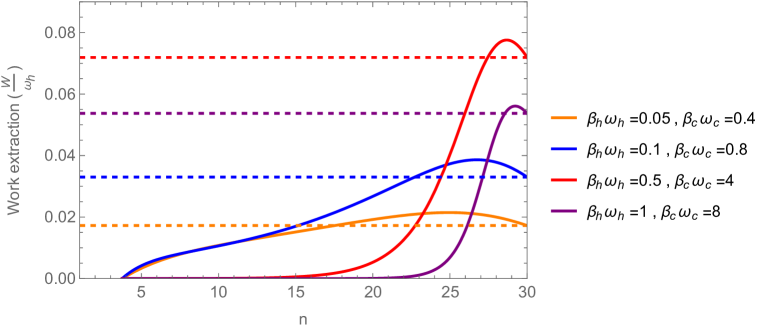
Figure 7: This figure depicts the variation of the work produced by the catalyst assisted two-stroke engine with $n$ as formulated in Eq. (60) for different values of $\beta_{h}\omega_{h}$ and $\beta_{c}\omega_{c}$ with $\frac{\beta_{c}\omega_{c}}{\beta_{h}\omega_{h}}=8$. Here we have taken the dimension of catalyst is $30$. Therefore, $n>3.75$ we have positive work produced by the engine as it requires $\frac{d}{n}<\frac{\beta_{c}\omega_{c}}{\beta_{h}\omega_{h}}$ (See Eq. (44)). The dashed line represents the work produced by the two-stroke engine without a catalyst with the different values of $\beta_{h}\omega_{h}$ and $\beta_{c}\omega_{c}$. One can see from the plot that work produced by the engine can be enhanced due to catalyst taking certain values of $n$ for each pair of values of $\beta_{h}\omega_{h}$ and $\beta_{c}\omega_{c}$. On the other hand, from left to right the efficiency of the catalyst assisted two-stroke engine is decreasing as the efficiency is given by the formula $1-\frac{n\omega_{c}}{d\omega_{h}}$, whereas the efficiency of the two-stroke engine without catalyst is given by the Otto efficiency. Hence, at rightmost point of the $x$-axis (i.e., at $n=30$) the efficiency of the catalyst assisted two stroke engine matches with the Otto efficiency whereas for $n<30$ the efficiency is strictly greater than Otto efficiency. Therefore, due to catalysis one can obtain a simultaneous enhancement on the work produced by the engine and the efficiency.

Our analysis mostly centred around a particular simple permutation $\Pi_{\text{gen}}$ for work extraction. In the appendix E, we have formulated a convex program for maximizing work extraction for any arbitrary unitary operation subjected to condition of preserving the catalyst. It involves optimization of probability vector achieved from a fixed one via unistochastic matrix, which give rise to some non-linear constraints. This make the problem hard to solve. We have relaxed the optimization problem of by subjecting it to a bigger set of probability vector achieved from a fixed one via bistochastic matrix. This relaxation reduces the optimization problem to a linear programming problem. We have formulated the primal as well as dual linear program of this relaxing optimization problem whose solution provides the upper bound on the work produced by the catalyst assisted two stroke engine where the dimension of the hot and cold $d$-level system is restricted to $2$.

So, far our results regarding catalytic enhancements mainly focused on the smallest two-stroke engine where the dimension of the hot and the cold $d$-level system is two. Now we shall ask: Whether catalytic enhancements in efficiency can be ensured for the two-stroke heat engine where the dimension of the hot and the cold $d$-level system can be arbitrary? In the next section, we shall partially answer this question.

VI.2 Catalytic enhancement in efficiency of the the two-stroke engine consist of arbitrary dimensional hot and cold $d$-level system

In this section, we would like to investigate whether the presence of a catalyst always leads to the enhancement of efficiency for a two-stroke engine with arbitrary dimensional hot and cold $d$-level system? Addressing the question for two-stroke engine with arbitrary dimensional hot and cold $d$-level system presents a significant challenge, because to prove catalytic enhancements one needs to know the optimal efficiency of the corresponding non-catalytic two-stroke engine. Obtaining the optimal efficiency of a non-catalytic two-stroke engines in such scenarios are extremely difficult, as the size of the feasible set and number of considerable parameter grows factorially with dimension. So, we shall try to characterize some instances where the catalytic enhancements can be ensured.

Consider a non-catalytic two-stroke heat engine with arbitrary dimensional hot and cold $d$-level system. It starts in the initial state $\tau_{h}\otimes\tau_{c}$ and transforms to $\rho^{*}_{hc}$ that leads to the maximum efficiency $\eta^{*}$. There can be two possibilities:

1. $\rho^{*}_{hc}$ is a correlated state.

2. $\rho^{*}_{hc}$ is a product state.

Consider the final state $\rho^{*}_{hc}$ that leads to optimal efficiency in a non-catalytic scenario is a correlated state. Now, we would like to employ a result from theorem 1 of Ref. [6] that proves the existence of a catalyst in the state $\rho_{s}$ and a unitary $U$ such that

$$|\Tr_{s,h}\big{(}U(\rho_{s}\otimes\rho^{*}_{h,c})U^{\dagger}\big{)}\rangle\!\rangle\succ|\Tr_{h}(\rho^{*}_{h,c})\rangle\!\rangle,$$ (65)

$$\Tr_{s,c}\big{(}U(\rho_{s}\otimes\rho^{*}_{h,c})U^{\dagger}\big{)}=\Tr_{c}(\rho^{*}_{h,c}),\quad\text{and}\quad$$ (66)

$$\Tr_{h,c}\big{(}U(\rho_{s}\otimes\rho^{*}_{h,c})U^{\dagger}\big{)}=\rho_{s},$$ (67)

if and only if $\rho^{*}_{h,c}$ is correlated. Here $|(\cdot)\rangle\!\rangle$ denotes the spectrum of $(\cdot)$ and the preservability of the marginal state of the catalyst is given by Eq. (67). One can observe from Eq. (66), the final state of hot $d$-level system in the two-stroke heat engine in the catalytic scenario is same with the final state of hot $d$-level system in the non-catalytic scenario. Therefore, the transferred amount of the heat $Q_{h}$ is same in both cases. Using the definition of heat transferred and cold heat from Eq. (10) and Eq. (11), we can write efficiency as

$$\eta=1+\frac{Q_{c}}{Q_{h}}=1-\frac{\Tr(H_{c}\rho_{c})-\Tr(H_{c}\tau_{c})}{\Tr(H_{h}\tau_{h})-Tr(H_{h}\rho_{h})}.$$ (68)

Now, to attain the optimal efficiency the final marginal state of the cold $d$-level system in $\rho^{*}_{h,c}$ has to be passive. If it is non-passive then after implementation of unitary that transforms $\tau_{h}\otimes\tau_{c}$ to $\rho^{*}_{h,c}$, one can apply a local unitary $\mathbb{I}_{h}\otimes V_{c}$ on the cold $d$-level system which make the cold $d$-level system passive without altering the energy of the hot $d$-level system. This will increase the efficiency further as can be seen from Eq. (68). Using the same reasoning we can also say that final state of the cold $d$-level system also has to be passive to obtain the optimal efficiency in the catalyic scenario as well. Therefore, the final average energy of the cold $d$-level system is equals to the passive energy where passive energy of a state $\rho$ means the average energy of its passive version can be defined via the relation:

$$\min_{V\in\mathbb{U}(d)}\Tr(HV\rho V^{\dagger})=\Tr(H\rho_{p}):=E_{\text{pass}}(\rho).$$ (69)

Since the passive energy of a state is Schur-concave function which can be seen from the lemma 1 in the appendix of Ref. [6], therefore from Eq. (65) implies the final average energy of cold $d$-level system in the catalytic scenario, is lower than final average energy of cold $d$-level system in the non-catalytic scenario. Therefore, from Eq. (68) we conclude that efficiency of the two-stroke engine assisted with a catalyst is greater than the efficiency of the two-stroke engine in the absence of a catalyst.

Next, consider $\rho^{*}_{h,c}$ is a product state that leads to the optimal efficiency $\eta^{*}$ in the non-catalytic scenario. Here, we would like to employ the results from Ref. [8] where in Eq. $(8)$ they have constructed a permutation $S$ such that for any passive state $\rho_{P}$ that is not equal to the Gibbs state of the system, the following holds:

$$\Tr(H\rho_{P}) > \Tr\big(H(\Tr_{M}S(\rho_{P}\otimes\rho_{M})S^{\dagger})\big{missing})$$ (70)

$$\rho_{M} = \Tr_{M}\big{(}S(\rho_{P}\otimes\rho_{M})S^{\dagger}\big{)}.$$ (71)

In other words, $S$ allows to reduce the average energy of a passive state which is not Gibbs state, using a catalyst. By inspecting Eq. (68), we see that to achieve maximal efficiency the final state of the hot and cold $d$-level system has to be passive (One can use a similar argument as earlier to conclude the hot $d$-level system also has to be in a passive state to obtain the optimal efficiency). Now, if the final state of the hot or cold $d$- level system $\rho^{*}_{h,c}$ is not thermal, then we can apply the permutation $S$ given in Eq. (70) on that non-thermal passive state and a catalyst solely. This results in reducing the average energy of that non-thermal passive state further, without any change in the average energy of the rest of the components. This would lead to the enhancement of the efficiency of the the two-stroke heat engines.

The only case which is left to be answered is when $\rho^{*}_{h,c}$ is a product of two Gibbs state. Note that, when the dimension of the hot and cold $d$-level system is equals to $2$, we have seen that $\rho^{*}_{h,c}$ became equals to $(\tau_{c}\otimes\tau_{h})_{h,c}$ (One can easily check this by applying the optimal permutation given in Eq. (17) on the initial state $(\tau_{h}\otimes\tau_{c})_{h,c}$). Now, the state $\tau_{c}$ can be thought as the Gibbs state of the hot two-level system at inverse temperature $\tilde{\beta}_{h}=\frac{\beta_{c}\omega_{c}}{\omega_{h}}$. Similarly, the state $\tau_{h}$ can be thought as the Gibbs state of the cold two-level system at inverse temperature $\tilde{\beta}_{c}=\frac{\beta_{h}\omega_{h}}{\omega_{c}}$. As we have shown, in that case we can always obtain catalytic enhancements in the efficiency. But we believe in this particular case, to obtain the catalytic enhancements in the efficiency for two-stroke engine with arbitrary dimensional hot and cold $d$-level system, one needs to figure out what is the optimal efficiency in the non-catalytic scenario first.

So, we summarize the results on the catalytic enhancement in the efficiency in the following table:

Final state $\rho^{*}_{h,c}$ leading	Catalytic
to optimal efficiency	Enhancement
in the non-catalytic scenario
Correlated	Yes
Product with either of the	Yes
$d$-level system is passive
but not Gibbs
Product with both of the	Yes
$d$-level system is Gibbs
when $d=2$
Product with both of the	?
$d$-level system is Gibbs
with $(d>2)$

VI.3 Correlation between the catalyst and the hot and cold two level system in the final state

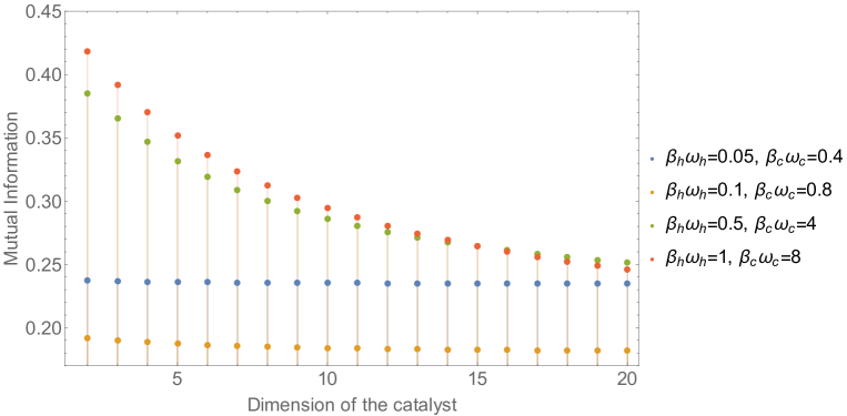
Figure 8: This figure depicts the variation of mutual information between the catalyst and the hot and cold two-level with dimension of the catalyst $d$ for the simple permutation formulated in Eq. (36). We see that with increase of dimension mutual information reduces.

In this section, we briefly address how much correlation between the catalyst and the hot and cold two-level system is created in order to obtain the efficiency $1-\frac{\omega_{c}}{d\omega_{h}}$. In particular, we shall calculate the mutual information that encapsulates the correlation between the catalyst and the hot and cold two-level system. We proceed from the definition of mutual information

$$I(s:h,c)=S(\rho_{s})+S(\rho_{h,c})-S(\rho^{f}_{s,h,c}).$$ (72)

Since, from the description of two-stroke thermal machines outlined in $\rho^{f}_{s,h,c}=U(\rho^{i}_{s,h,c})U^{\dagger}=U(\rho_{s}\otimes\tau_{h}\otimes\tau_{c})U^{\dagger}$ we obtain

$$I(s:h,c)=S(\rho_{s})+S(\rho_{h,c})-S(\rho^{i}_{s,h,c})$$ (73)

$$= S(\rho_{s})+S(\rho_{h,c})-S(\rho_{s})-S(\tau_{h})-S(\tau_{c})$$

$$= S(\rho_{h,c})-S(\tau_{h})-S(\tau_{c})$$

The general expression of the mutual information is very tedious. We have depicted the mutual information with dimension for certain cases in Fig. 8. We see that mutual information decreases with dimension of the catalyst.

VII Conclusion

In our study, we present protocols aimed at boosting the efficiency of two-stroke heat engines through the assistance of a catalyst. Our approach involved devising a comprehensive thermodynamic framework for a two-stroke thermal machine operating with and without a catalyst. Our primary focus was on the smallest version of these engines, consisting of two two-level systems operating at two distinct temperatures. Without a catalyst, the optimal efficiency for such a two-stroke heat engine aligns with the Otto efficiency. In the accompanying paper in Ref. [46], a protocol was introduced to surpass the optimal Otto efficiency by incorporating a catalyst into the two-stroke engine. In particular, the accompanying work in Ref. [46] outlines a protocol resulting in an efficiency of $1-\frac{\omega_{c}}{d\omega_{h}}$ for a two-stroke engine when a catalyst is present.

Here we have identified a specific set of permutations, called simple permutations, where the efficiency expressed by $1-\frac{\omega_{c}}{d\omega_{h}}$ stands as the optimal value. Moreover, within a subset of these simple permutations, we conducted an analysis of the trade-off between the work produced by the engine per cycle and the efficiency. The intricate structure of the feasible set for optimizing work restricts our ability to offer only an upper bound on the work produced by a catalyst-assisted two-stroke engine using linear programming methodologies. On the other hand, formulating a linear program for optimizing efficiency becomes challenging due to its nonlinear structure. Finally, our exploration leads us to identify certain scenarios where catalytic enhancements reliably guarantee efficiency enhancements in a two-stroke heat engine.

This works opens up a numerous interesting questions: First, whether incorporating a catalyst always allows us to surpass the optimal efficiency of the two-stroke engines without a catalyst? In this work we have shown that catalytic enhancement in the efficiency of the two-stroke heat engine is always possible if the optimal efficiency is achieved in the non-catalytic scenario for the final state having correlations between the hot and cold $d$-level system. Additionally, we have established that catalytic enhancements in efficiency are achievable even when the optimal efficiency in the non-catalytic scenario is achieved for the final state of the hot and cold $d$-level system is a product of two states, where at least one of them is not Gibbs. Finally, our research proves that when the dimension of the hot and cold $d$-level system is two (i.e. $d=2)$, catalytic enhancements in efficiency can be obtained, if the optimal efficiency in the non-catalytic scenario occurs for a final state of the hot and cold $2$-level system which is product of two Gibbs state at two different temperatures. Now whether it is true for any dimension is still unknown but we conjectured that it is always possible to obtain a catalytic enhancement.

Second, whether incorporating a catalyst leads to enhancement in the performance of other thermodynamic devices and tasks? The results presented in this paper deals with the catalytic enhancement of the efficiency of the two-stroke heat engine. Analogously, using the methodologies developed for the two-stroke heat engines, one can address the problem of enhancing the efficiency of the cooler and the heat pump [7, 6]. Furthermore, one can investigate to role of the catalyst in other tasks such as generation of non-classical light [62], and the simulation of non-markovianity via Markovian dynamics. [63].

Finally, how to bridge the gap between the two-stroke heat engines and self-contained heat engines? In this paper, our focus has been on stroke-based heat engines, where work extraction and rethermalization occur in distinct, discrete time intervals. It raises the question: whether the enhancement in the efficiency for the two-stroke heat engines are also valid for self-contained heat engines, where thermalization and work extraction happen simultaneously and continuously? We anticipate that there will be a correspondence between the two-stroke discrete heat engine and the self-contained heat engine. In particular, one can expect to show the catalytic enhancement in the efficiency for self-contained thermal machine as well. Note that, the analysis of the self-contained heat engine allows us compute power or rate of work produced by the engine in time whereas, the proposed two-stroke heat engine provides average work per cycle. After establishing the correspondence between the two-stroke discrete heat engine and the self-contained heat engine rigorously, one can ask: what is the minimum time required by the self-contained heat engine to complete a cycle? This connection between the discrete two-stroke heat engine and the continuous self-contained heat engine not only provides interesting theoretical research direction but also provides insights into the experimental realization of two-stroke heat engines. In Ref. [64], an experimental implementation of the self-contained refrigerator within the framework of cavity quantum electrodynamics was proposed. Furthermore, a more recent work detailed in Ref. [65] addresses the construction of a self-contained refrigerator using superconducting circuits. Hence, we believe that designing a two-stroke heat engine, with or without a catalyst, can also be achieved within the frameworks of cavity QED and superconducting circuits.

Appendix A Thermodynamical framework

A.1 Modes of operation for the two-stroke thermal machines

We can classify the two-stroke thermal machines into three distinct modes based on the work and heat that is associated with its transformation.

1. Heat engines: A two-stroke thermal machine work as a heat engine if the work associated with it is transformation is positive, i.e., $W>0$. This means the thermal machine is producing the work using the temperature difference between the hot and the cold $d$-level system.

2. Coolers: On the other hand, a two-stroke thermal machine is classified as a cooler if the work associated with it is negative i.e., $W<0$ whereas the cold heat $Q_{c}>0$. This means that thermal machine utilizes the work in order to cool the cold $d$-level system by releasing heat into a cold bath.

3. Heat Pumps: Lastly, the two-stroke thermal machine operates as a heat pump when the work associated with it is non-positive, indicated as $W\leq 0$, while the heat consumed by the thermal machine is positive, denoted as $Q_{h}\geq 0$.

A.2 Derivation of the second law for the two-stroke thermal machines

In this section, we will formulate the second law of thermodynamics for the two-stroke thermal machines. In particular we shall show for a two-stroke thermal machine operating as an heat engine, must withdraw a positive amount of heat from the hot bath. Furthermore, we will establish the efficiency of a two-stroke heat engine is upper bounded by the Carnot efficiency. On the other hand, when the two-stroke thermal machine operates as a cooler, we will prove that its efficiency is, in turn, lower bounded by the Carnot efficiency.

We begin by recalling that the initial state of the two-stroke thermal machine as $\rho^{i}_{s,h,c}=\rho_{s}\otimes\tau_{h}\otimes\tau_{c}$ that evolves via a unitary transformation $U$ that preserves the state of the catalyst as stated definition 1. Now, we introduce a class of transformation on the catalyst, the hot and and cold $d$-level system called entropy non-decreasing transformation. This concept will be crucial to establish the thermodynamic framework for the two-stroke thermal machine.

Definition 4 (Entropy non-decreasing transformation).

An entropy non-decreasing transformation $\mathcal{U}$ is a complete positive trace preserving (CPTP) map that acts on the combined state of the catalyst, the hot and the cold $d$-level system $\sigma_{s,h,c}$, such that

$$S(\rho_{s,h,c})\leq S(\mathcal{U}(\rho_{s,h,c})),$$ (74)

where $S(\cdot)$ denotes the von Neumann entropy which is defined as

$$S(\cdot)=-\Tr((\cdot)\ln(\cdot)).$$ (75)

Clearly, any unitary operation is an entropy non-decreasing transformation as it preserves the von-Neumann entropy. Moreover, the set of states that can be achieved from a fixed state $\rho$ is convex. This can be seen as follows:

$$S(\lambda\mathcal{U}_{1}(\rho)+(1-\lambda)\mathcal{U}_{2}(\rho))\geq\lambda S(\mathcal{U}_{1}(\rho))+(1-\lambda)S(\mathcal{U}_{2}(\rho))\\ \geq\lambda S(\rho)+(1-\lambda)S(\rho)=S(\rho).$$ (76)

The main motivation for introducing these class of operations is to consider a generic set of transformations on the Hilbert space of catalyst, hot and cold $d$-level system that encompasses any arbitrary unitary transformations on them. In the next section, we shall see that optimization of the efficiency as well as work produced by the two-stroke thermal engines boils down to the set of all states that can be achieved via unitary transformation from the initial state. Furthermore, employing the convexity of the achievable states via the entropy non-decreasing transformation allows us to write the extraction of work as a linear program.

Now, we shall show the second law holds even if the combined state $\rho_{s}\otimes\tau_{h}\otimes\tau_{c}$ evolves via entropy non-decreasing transformation which naturally gives the second law if the combined state evolves via a unitary.

Lemma 6 (Clausius inequality).

For any two-stroke thermal machine whose joint initial state $\rho^{i}_{s,h,c}$ of the catalyst, the hot and the cold $d$-level system transforms via an entropy non-decreasing transformation to the final state $\rho^{f}_{s,h,c}$ satisfies the following inequality:

$$\beta_{h}Q_{h}+\beta_{c}Q_{c}\leq 0.$$ (77)

Proof.

The proof of the lemma follows from the non-negativity of relative entropy i.e

$$D(\rho^{f}_{s,h,c}\|\rho^{i}_{s,h,c}):=-S(\rho^{f}_{s,h,c})-\Tr(\rho^{f}_{s,h,c}\log\rho^{i}_{s,h,c})\geq 0$$

$$\Rightarrow -S(\rho^{i}_{s,h,c})-\Tr(\rho^{f}_{s,h,c}\log\rho^{i}_{s,h,c})-\delta\geq 0$$

$$\Rightarrow \Tr\big((\rho^{i}_{s,h,c}-\rho^{f}_{s,h,c})\log\rho^{i}_{s,h,c}\big{missing})-\delta\geq 0$$

$$\Rightarrow \Tr\big((\rho^{i}_{s,h,c}-\rho^{f}_{s,h,c})(\log\rho_{s}+\log\tau_{h}+\log\tau_{c})\big{missing})-\delta\geq 0$$

$$\Rightarrow \Tr\big((\rho^{i}_{s,h,c}-\rho^{f}_{s,h,c})(-\beta_{h}H_{h}-\beta_{c}H_{c})\big{missing})-\delta\geq 0$$

$$\Rightarrow -(\beta_{h}Q_{h}+\beta_{c}Q_{c})-\delta\geq 0$$

$$\Rightarrow 0\geq-\delta\geq(\beta_{h}Q_{h}+\beta_{c}Q_{c}).$$

Here, to write the first implication we use the definition of the entropy non-decreasing transformation with $\delta>0$, to write the second implication we use simply the definition of von-Neumann entropy, to write the third implication we uses the fact that the state $\rho^{i}_{s,h,c}=\rho_{s}\otimes\tau_{h}\otimes\tau_{c}$. Now, in order to write the fourth implication, we use the fact that marginal state of the catalyst in the initial and the final state are same, and the definition of $\tau_{h}$ and $\tau_{c}$ from Eq. (3). ∎

Note that, the second law inequality given in Eq. (77) holds even if we consider a two-stroke thermal machines that does not contain any catalyst. This can be seen easily from the derivation. Next, using the Clausius inequality from lemma 6, we shall prove that the transferred amount of heat from the hot bath is always positive for the two-stroke thermal machine operating as an engine.

Proposition 7 (Positivity of heat transfer in the two-stroke heat engines).

Any two-stroke thermal machine operating as an engine whose joint initial state $\rho^{i}_{s,h,c}$ of the catalyst, the hot and the cold $d$-level system transforms via an entropy non-decreasing transformation to the final state $\rho^{f}_{s,h,c}$, always leads to a positive amount of heat transfer from the hot heat bath i.e.,

$$W>0\Rightarrow Q_{h}>0.$$ (78)

Proof.

This proof directly follows from second law inequality given in Eq. (77), and the fact that work associated with thermal machine operated as an engine is always positive as defined in Sec. A.1. The second law inequality in Eq. (77) can be rewritten as

$$-\frac{\beta_{h}}{\beta_{c}}Q_{h}\geq Q_{c}.$$ (79)

On the other hand, positivity of work implies

$$W=Q_{h}+Q_{c}>0\Rightarrow Q_{h}(1-\frac{\beta_{h}}{\beta_{c}})>0\Rightarrow Q_{h}>0,$$ (80)

where we use the definition of work from Eq. (12), the inequality from Eq. (79) and the fact $\beta_{c}>\beta_{h}$, to draw the implication in Eq. (80). ∎

So, from this proposition, we conclude that if the two-stroke thermal machines operate as an engine, then it should withdraw a positive amount of heat from the hot heat bath to produce work. Finally, employing lemma 6 and theorem 7, we shall establish the ordering among the efficiency between different modes of the two-stroke thermal machines.

Proposition 8 (Ordering of the efficiency between different modes of thermal machines).

The following statements holds true for any two-stroke thermal machines operating with the efficiency $\eta$:

1. $0<\eta\leq(1-\frac{\beta_{h}}{\beta_{c}})$ if and only if the two-stroke thermal machines operates as an engine.

2. $\eta\geq(1-\frac{\beta_{h}}{\beta_{c}})$ if and only if the two-stroke thermal machines operates as a cooler.

3. $\eta\leq 0$ if and only if the two-stroke thermal machines operates as a heat pump.

Proof.

From theorem 7, we see that for two-stroke thermal machine operated as an engine, the transferred amount of heat from the hot bath $Q_{h}$ is positive which proves the efficiency is positive. On the other hand, from the second law inequality given in Eq. (79), and using the fact $Q_{h}>0$ we can derive $-\frac{\beta_{h}}{\beta_{c}}\geq\frac{Q_{c}}{Q_{h}}$. This implies $\eta=1+\frac{Q_{c}}{Q_{h}}\leq 1-\frac{\beta_{h}}{\beta_{c}}$.

On the other hand, for the two stroke thermal machine operated in the cooling mode have $Q_{h}<0$ (see the Sec. A.1). Therefore, the second law inequality given in Eq. (79) can be reduced to $-\frac{\beta_{h}}{\beta_{c}}\leq\frac{Q_{c}}{Q_{h}}$ which implies $\eta=1+\frac{Q_{c}}{Q_{h}}\geq 1-\frac{\beta_{h}}{\beta_{c}}$.

Finally, for the two stroke thermal machine operated as an heat pump have $W<0$ and $Q_{h}>0$ as defined in Sec. A.1 which makes its efficiency $\eta\leq 0$. ∎

Thus, the corollary 8 sets the ordering the efficiency of the different modes of the thermal machine starting with the same initial state $\rho_{s,h,c}^{i}=\rho_{s}\otimes\tau_{h}\otimes\tau_{c}$ in the following manner:

$$\eta^{\text{max}}_{\text{heat pump}}\leq\eta^{\text{min}}_{\text{heat engine}}\leq\eta^{\text{max}}_{\text{heat engine}}\leq\eta^{\text{min}}_{\text{cooler}},$$ (81)

where $\eta^{\text{max}}_{x}$ and $\eta^{\text{min}}_{x}$ denotes the maximum and minimum efficiency when the two-stroke thermal machine operates in the mode $x$. It is important to emphasize that Eq. (81) only holds for fixed initial state of the thermal machine. Hence, we can not use this inequality directly to compare in a two-stroke thermal machine with catalyst where the initial state of the catalyst varies with the transformation acting on the initial state of the thermal machine. This results changing the initial state of thermal machine with the change of the transformation that is implemented.

Since both proposition 7 and proposition 8 both stems from the Clausius inequality established in lemma 6 that holds true for the two-stroke thermal machines without a catalyst, these results in theorem 7 and corollary 8 also hold true for such machines. As the initial state for the two-stroke thermal machine in the absence of the catalyst is $\rho^{i}_{h,c}=\tau_{h}\otimes\tau_{c}$ which does not depends on the transformation, the inequality given in Eq. (81) applies directly. We shall use this inequality later to optimize the efficiency of two-stroke heat engines.

Appendix B Proof of theorem 1

Proof.

Starting from Eq. (9), we can write work produced by a two-stroke heat engine without catalyst as $W=\Tr\big((H_{h}+H_{c})(\rho^{i}_{h,c}-\rho^{i}_{h,c})\big{missing})$. It is straightforward to see that $W$ is a linear function of $\rho^{i}_{h,c}$ and does not depend on the off-diagonal terms of the state $U\rho^{i}_{h,c}U^{\dagger}$. Thus we can write work produced by this engine as

$$W=\Tr\Big((H_{h}+H_{c})\big{(}\rho_{h,c}^{i}-\mathcal{D}(U\rho_{h,c}^{i}U^{\dagger})\big{)}\Big{missing}),$$ (82)

where $\mathcal{D}(\cdot)$ denotes the dephasing in the eigenbasis of the Hamiltonian $H_{h}+H_{c}$. According to Schur-Horn theorem, $|\mathcal{D}(U\rho_{h,c}^{i}U^{\dagger})\rangle\!\rangle=B|\rho_{h,c}^{i}\rangle\!\rangle$ where $|\cdot\rangle\!\rangle$ denotes the spectrum of $(\cdot)$, and $B$ is some bistochastic matrix. Therefore, it is straight-forward to rewrite the expression of work $W$ in Eq. (82) as

$$W=\langle\!\langle H_{h}+H_{c}|\rho_{h,c}^{i}\rangle\!\rangle-\langle\!\langle H_{h}+H_{c}|B|\rho_{h,c}^{i}\rangle\!\rangle.$$ (83)

From Birkhoff-vonNeumann theorem we know that one can decompose any bistochastic matrix as a convex sum of permutations i.e $B=\sum_{i}\alpha_{i}\Pi_{i}$. Therefore, we can have the following:

$$W = \sum_{k}\alpha_{k}\Big{(}\langle\!\langle H_{h}+H_{c}|\rho_{h,c}^{i}\rangle\!\rangle-\langle\!\langle H_{h}+H_{c}|\Pi_{k}|\rho^{i}_{h,c}\rangle\!\rangle\Big{)}$$ (84)

$$\leq \langle\!\langle H_{h}+H_{c}|\rho_{h,c}^{i}\rangle\!\rangle-\langle\!\langle H_{h}+H_{c}|\Pi^{*}|\rho^{i}_{h,c}\rangle\!\rangle,$$

where $\Pi^{*}$ is the permutation such that

$$\forall k,\quad\langle\!\langle H_{h}+H_{c}|\Pi_{k}|\rho^{i}_{h,c}\rangle\!\rangle\geq\langle\!\langle H_{h}+H_{c}|\Pi^{*}|\rho^{i}_{h,c}\rangle\!\rangle:=W_{\Pi^{*}}.$$ (85)

Next, in order to optimize the efficiency we proceed by writing efficiency as follows:

$$\eta = \sum_{k}\frac{\alpha_{k}Q_{\Pi_{k}}}{Q_{h}}\frac{W_{\Pi_{k}}}{Q_{\Pi_{k}}}=\sum_{k}\frac{\alpha_{k}Q_{\Pi_{k}}}{Q_{h}}\eta_{\Pi_{k}},$$ (86)

where

$$W_{\Pi_{k}} = (\langle\!\langle H_{h}+H_{c}|\rho^{i}_{h,c}\rangle\!\rangle-\langle\!\langle H_{h}+H_{c}|\Pi_{k}|\rho^{i}_{h,c}\rangle\!\rangle),$$ (87)

$$Q_{\Pi_{k}} = (\langle\!\langle H_{h}|\rho^{i}_{h,c}\rangle\!\rangle-\langle\!\langle H_{h}|\Pi_{k}|\rho^{i}_{h,c}\rangle\!\rangle),$$ (88)

$$Q_{h} = (\langle\!\langle H_{h}|\rho^{i}_{h,c}\rangle\!\rangle-\langle\!\langle H_{h}|B|\rho^{i}_{h,c}\rangle\!\rangle)=\sum_{k}\alpha_{k}Q_{\Pi_{k}}.$$ (89)

Note that, Eq. (86) is not a convex sum because there may exist some $k$ for which $Q_{\Pi_{k}}$ is negative. On the other hand $Q_{h}>0$ due to proposition 7. Furthermore, employing proposition 7 again we infer that $Q_{\Pi_{j}}>0$ whenever $W_{\Pi_{j}}>0$, which implies any permutation appeared in Eq. (86) must belong to either of the following sets

$$\mathcal{J}_{E}:=\{j\quad\text{such that}\quad W_{\Pi_{j}}>0\},$$ (90)

$$\mathcal{J}_{C}:=\{j\quad\text{such that}\quad W_{\Pi_{j}}<0\;\text{and}\;Q_{\Pi_{j}}<0\},$$ (91)

$$\mathcal{J}_{H}:=\{j\quad\text{such that}\quad W_{\Pi_{j}}<0\;\text{and}\;Q_{\Pi_{j}}\geq 0\}.$$ (92)

This simply means for $j\in\mathcal{J}_{E}$ the permutation $\Pi_{j}$ corresponds to engine mode, for $j\in\mathcal{J}_{C}$ the permutation $\Pi_{j}$ corresponds to cooling mode, and for $j\in\mathcal{J}_{H}$ the permutation $\Pi_{j}$ corresponds to heat pump mode. Hence, the expression of efficiency given in Eq. (86) reduces to

$$\eta=\sum_{j\in\mathcal{J}_{E}}\frac{\alpha_{j}Q_{\Pi_{j}}}{Q_{h}}\eta_{\Pi_{j}}+\sum_{j\in\mathcal{J}_{C}}\frac{\alpha_{j}Q_{\Pi_{j}}}{Q_{h}}\eta_{\Pi_{j}}+\sum_{j\in\mathcal{J}_{H}}\frac{\alpha_{j}Q_{\Pi_{j}}}{Q_{h}}\eta_{\Pi_{j}}.$$ (93)

Now let us define

$$\eta^{\text{max}}_{\mathcal{J}_{x}}:=\max_{\Pi_{j}\in\mathcal{J}_{x}}\eta_{\Pi_{j}};\quad\eta^{\text{min}}_{\mathcal{J}_{x}}:=\min_{\Pi_{j}\in\mathcal{J}_{x}}\eta_{\Pi_{j}}$$

where $x\in\{E,H,C\}$. Thus we can write the following inequality

$$\eta\leq\sum_{j\in\mathcal{J}_{E}}\frac{\alpha_{j}Q_{\Pi_{j}}}{Q_{h}}\eta^{\text{max}}_{\mathcal{J}_{E}}+\sum_{j\in\mathcal{J}_{C}}\frac{\alpha_{j}Q_{\Pi_{j}}}{Q_{h}}\eta^{\text{min}}_{\mathcal{J}_{C}}$$ (94)

$$+ \sum_{j\in\mathcal{J}_{H}}\frac{\alpha_{j}Q_{\Pi_{j}}}{Q_{h}}\eta^{\text{max}}_{\mathcal{J}_{H}},$$

where we use the fact $Q_{\Pi_{j}}>0$ for all $j\in\mathcal{J}_{E}$ and for all $j\in\mathcal{J}_{H}$ whereas $Q_{\Pi_{j}}<0$ for all $j\in\mathcal{J}_{C}$ as defined in Eq. (90). Due to inequality at Eq. (81) which is true for any unitaries that transforms the state of the thermal machine during work stroke, we can write

$$\eta^{\text{max}}_{\mathcal{J}_{H}}\leq\eta^{\text{max}}_{\text{heat pump}}\leq\eta^{\text{min}}_{\text{heat engine}}\leq\eta^{\text{max}}_{\mathcal{J}_{E}}\leq\eta^{\text{min}}_{\text{cooler}}\leq\eta^{\text{min}}_{\mathcal{J}_{C}},$$ (95)

which allows us to further bound the inequality given in Eq. (94)

$$\eta\leq\sum_{j\in\mathcal{J}_{E}}\frac{\alpha_{j}Q_{\Pi_{j}}}{Q_{h}}\eta^{\text{max}}_{\mathcal{J}_{E}}+\sum_{j\in\mathcal{J}_{C}}\frac{\alpha_{j}Q_{\Pi_{j}}}{Q_{h}}\eta^{\text{min}}_{\mathcal{J}_{C}}$$ (96)

$$+ \sum_{j\in\mathcal{J}_{H}}\frac{\alpha_{j}Q_{\Pi_{j}}}{Q_{h}}\eta^{\text{max}}_{\mathcal{J}_{H}}\leq\eta^{\text{max}}_{\mathcal{J}_{E}}\Big{(}\sum_{j}\frac{\lambda_{j}Q_{\Pi_{j}}}{Q_{h}}\Big{)}$$

$$= \eta^{\text{max}}_{\mathcal{J}_{E}},$$

which completes the proof. ∎

Thus, from the proof of the theorem 1, we see that optimal efficiency for a two-stroke heat engine is achieved for some permutation. In other words, if the initial state transformed via some unitary $\tilde{U}$ such that $|\tilde{\mathcal{D}}(\tilde{U}\rho^{i}_{h,c}\tilde{U}^{\dagger})\rangle\!\rangle=\tilde{B}|\rho^{i}_{h,c}\rangle\!\rangle$ where $\tilde{B}$ is some non-trivial mixture of permutations, then $\tilde{U}$ can not lead to optimal production of work or the efficiency. We shall see in the next section that theorem 1 extremely simplifies the calculation of optimal efficiency for the smallest the two-stroke heat engine that constitutes of two-level systems only. On the other hand, the optimization of work is much easier for any given initial state $\tau_{h}\otimes\tau_{c}$, because work will be maximized for the permutation that leads to the passive version of the state $\tau_{h}\otimes\tau_{c}$ [16].

Appendix C Smallest possible two-stroke heat engine without a catalyst

In this section, we shall analyze the performance of the smallest possible two-stroke heat engine where the hot and cold $d$ level systems are qubit. The the hot and cold baths are in equilibrium w.r.t. Hamiltonian $H_{h}=\omega_{h}|1\rangle\langle 1|$ and $H_{c}=\omega_{c}|1\rangle\langle 1|$ and inverse temperature $\beta_{h}$ and $\beta_{c}$. Therefore, the combined state of hot and the cold bath is given as

$$|\rho^{i}_{h,c}\rangle = \frac{1}{1+a_{h}}(1\;\;a_{h})^{T}\otimes\frac{1}{1+a_{c}}(1\;\;a_{c})^{T},$$ (97)

$$= \frac{1}{(1+a_{h})(1+a_{c})}(1\;\;a_{c}\;\;a_{h}\;\;a_{c}a_{h})^{T}.$$

where $a_{h}=e^{-\beta_{h}\omega_{h}}$ and $a_{c}=e^{-\beta_{c}\omega_{c}}$. The total Hamiltonian is given as $H=H_{h}\otimes\mathbb{I}+\mathbb{I}\otimes H_{c}$, thus

$$|H\rangle=(0\;\;\omega_{c}\;\;\omega_{h}\;\;\omega_{c}+\omega_{h})^{T};$$

$$\quad|H_{h}\rangle=(0\;\;0\;\;\omega_{h}\;\;\omega_{h})^{T}.$$ (98)

From the initial state given in Eq. (97), we easily see that only one permutation $\Pi$ leads to positive value for extraction of work that is given below:

$$\Pi=|0,0\rangle\langle 0,0|+|0,1\rangle\langle 1,0|+|1,0\rangle\langle 0,1|+|1,1\rangle\langle 1,1|.$$ (99)

This results the following final state,

$$|\rho^{i}_{h,c}\rangle = \frac{1}{(1+a_{h})(1+a_{c})}(1\;\;a_{c}\;\;a_{h}\;\;a_{c}a_{h})^{T},$$

$$\xrightarrow{\Pi} \frac{1}{(1+a_{h})(1+a_{c})}(1\;\;a_{h}\;\;a_{c}\;\;a_{c}a_{h})^{T}:=|\rho^{f}_{h,c}\rangle.$$

Therefore, the optimal work production is given by

$$W = \Tr\Big(H(\rho^{i}_{h,c}-\rho^{f}_{h,c})\Big{missing})=\langle H|\rho^{i}_{h,c}\rangle-\langle H|\rho^{f}_{h,c}\rangle$$ (101)

$$= (a_{h}-a_{c})(\omega_{h}-\omega_{c}).$$

Similarly, the amount of heat exchanged from the hot reservoir can be calculated as

$$Q_{h}=\Tr\Big(H_{h}\otimes\mathbb{I}(\rho^{i}_{h,c}-\rho^{f}_{h,c})\Big{missing}) = \langle H_{h}|\rho^{i}_{h,c}\rangle-\langle H_{h}|\rho^{f}_{h,c}\rangle$$ (102)

$$= (a_{h}-a_{c})\omega_{h}.$$

For this permutation, efficiency is given by the Otto efficiency

$$\eta=\frac{W}{Q}=1-\frac{\omega_{c}}{\omega_{h}},$$ (103)

which is the optimal efficiency.

Appendix D Proof of the proposition 2

Proof.

We begin by rewriting the definition of work and the efficiency of the two-stroke heat engine given in Eq. (12) and Eq. (13) i.e,

$$W=Q_{c}+Q_{h}\;,\;\quad\eta=1+\frac{Q_{c}}{Q_{h}}.$$ (104)

From the above equations we can infer that in order to prove the claim it is enough to construct an unitary $\tilde{U}$ and a catalyst $\tilde{\rho}_{s}$ that gives the transferred amount of heat $\tilde{Q}_{h}$ and the cold heat $\tilde{Q}_{c}$ exactly same as $Q_{h}$ and $Q_{c}$ i.e., $\tilde{Q}_{h}=Q_{h}$ and $\tilde{Q}_{c}=Q_{c}$. Let us assume the initial state of the two-stroke thermal machine $\rho_{s}\otimes\tau_{h}\otimes\tau_{c}$ transforms via an unitary $U$, we have

$$Q_{h} = \Tr\big(H_{h}(\rho_{s}\otimes\tau_{h}\otimes\tau_{c}-U(\rho_{s}\otimes\tau_{h}\otimes\tau_{c})U^{\dagger})\big{missing})$$

$$Q_{c} = \Tr\big(H_{c}(\rho_{s}\otimes\tau_{h}\otimes\tau_{c}-U(\rho_{s}\otimes\tau_{h}\otimes\tau_{c})U^{\dagger})\big{missing})$$ (105)

$$\text{such that }\Tr_{h,c}U(\rho_{s}\otimes\tau_{h}\otimes\tau_{c})U^{\dagger}=\rho_{s}.$$

One can diagonalize $\rho_{s}=K\rho_{s}^{D}K^{\dagger}$ where $K$ is unitary and $\rho_{s}^{D}$ is a diagonal matrix that contains the eigenvalues of $\rho_{s}$. Now we choose

$$\tilde{\rho}_{s}=\rho^{D}_{s}\quad,\quad\tilde{U}=K^{\dagger}UK.$$ (106)

Then one can write

$$\tilde{Q}_{h} = \Tr\big(H_{h}(\tilde{\rho}_{s}\otimes\tau_{h}\otimes\tau_{c}-\tilde{U}(\tilde{\rho}_{s}\otimes\tau_{h}\otimes\tau_{c})\tilde{U}^{\dagger})\big{missing})$$ (110)

$$=$$

$$=$$

$$=\Bigg{(}p_{1}a_{h}^{m}-\frac{\Delta P}{{\cal N}}\Big{(}\frac{1-a_{h}^{m}}{1-a_{h}}\Big{)}\Bigg{)}\Big{(}\frac{a_{h}}{a_{c}}\Big{)}^{t}-\frac{\Delta P}{{\cal N}a_{c}}\Bigg{(}\frac{(\frac{a_{h}}{a_{c}})^{t}-1}{(\frac{a_{h}}{a_{c}})-1}\Bigg{)}$$

$$p_{1}=p_{m+n}\frac{a_{h}}{a_{c}}-\frac{\Delta P}{{\cal N}a_{c}}.$$

From the normalization of the probability, we can write

$$\sum_{x=2}^{m+n}p_{x} = \sum_{x=2}^{m+1}p_{x}+\sum_{x=m+2}^{m+n}p_{x}=\sum_{s=1}^{m}p_{s+1}+\sum_{t=1}^{n-1}p_{m+t+1}$$ (111)

$$= 1-p_{1}.$$

Substituting the value of $p_{x}$ from Eq. (LABEL:G8) and (LABEL:G10) in Eq. (111), we obtain $p_{1}$ in terms of $\Delta P$. In order to get the solution of $\Delta P$, we substituted the obtained expression of $p_{1}$ in terms of $\Delta P$ in Eq. (110) and solved it. This gives

$$\Delta P=\frac{1}{f(a_{h},a_{c},m,n)}{\cal N}(a_{h}^{m+n}-a_{c}^{n}),$$ (112)

with

$$f(a_{h},a_{c},m,n)=\frac{1}{a_{c}^{n}(a_{h}-a_{c})^{2}(1-a_{h})^{2}}\Bigg{[}a_{c}^{2}\Big{\{}m-a_{h}(m+1-a_{h}^{m})+\bigg{(}\frac{a_{h}}{a_{c}}\bigg{)}^{n}\Big{(}a_{h}+a_{h}^{m}\big{(}-m+ma_{h}-a_{h}\big{)}\Big{)}\Big{\}}$$

$$+a_{h}\bigg{\{}-1-n+ma_{h}+2na_{h}-(m+n)a_{h}^{2}+a_{h}^{m}+\bigg{(}\frac{a_{h}}{a_{c}}\bigg{)}^{n}\bigg{(}1+a_{h}^{m}\Big{(}n-1-(m+2n)a_{h}+(m+n)a_{h}^{2})\Big{)}\bigg{)}\bigg{\}}$$

$$+a_{c}\bigg{\{}n+a_{h}\Big{(}(2m+n)a_{h}-2a_{h}^{m}-2(m+n-1)\Big{)}-\bigg{(}\frac{a_{h}}{a_{c}}\bigg{)}^{n}\bigg{(}2a_{h}+a_{h}^{m}\Big{(}n-2a_{h}(m+n+1)+(2m+n)a_{h}^{2}\Big{)}\bigg{)}\bigg{\}}\Bigg{]}.$$

Thus, employing Eq. (LABEL:eq:work_renewed) we get work as

$$W=\frac{{\cal N}\big{(}(m+n)\omega_{h}-n\omega_{c}\big{)}(a_{h}^{m+n}-a_{c}^{n})}{f(a_{h},a_{c},m,n)}.$$ (114)

On the other hand, the efficiency for such a simple permutation depicted in Fig. 5 can be calculated using Eq. (LABEL:QcQh) as follows:

$$\eta=1+\frac{Q_{c}}{Q_{h}}=1-\Big{(}\frac{n}{m+n}\Big{)}\frac{\omega_{c}}{\omega_{h}}.$$ (115)

Appendix E Work extraction as linear program

As we have mentioned earlier, the maximum amount of the work that can be produced by the two-stroke heat engine is a challenging task. Unlike non-catalytic scenario, we do not know whether the implementation of permutation on the initial state will lead to the optimal work extraction. In this section we shall try to provide an upper bound on the amount of work that can be produced by the engine in presence of a fixed catalyst as a linear program. In order to do so, we first write the initial state as

$$\rho^{i}_{s,h,c}=\rho_{s}\otimes\tau_{h}\otimes\tau_{c}=\sum_{i=1}^{d}p_{i}|i\rangle\langle i|\otimes\tau_{h}\otimes\tau_{c}.$$ (116)

and define the projector

$$M_{i}:=|i\rangle\langle i|\otimes\mathbb{I}_{h}\otimes\mathbb{I}_{c}.$$ (117)

For a given total Hamiltonian $H$ of the engine, and the initial state $\rho^{i}_{s,h,c}$, we can express the amount of produced work $W(\cdot)$ as a function of initial state $\rho^{i}_{s,h,c}$ via the following optimization problem:

maximize $$W(\rho^{i}_{s,h,c}):=\langle\!\langle H|\rho^{i}_{s,h,c}\rangle\!\rangle-\langle\!\langle H|B|\rho^{i}_{s,h,c}\rangle\!\rangle$$ (118)

subject to $$B_{xy}=|U_{xy}|^{2}\quad{\text{for some unitary $U$}}$$

$$\forall k\;\;\;\;\langle\!\langle M_{k}|B|\rho^{i}_{s,h,c}\rangle\!\rangle=\langle\!\langle M_{k}|\rho^{i}_{s,h,c}\rangle\!\rangle$$

The solution of the introduced linear program would give optimal work extracted from the system assisted by a catalyst. But, this problem is very hard to solve due to constraint $B_{xy}=|U_{xy}|^{2}$ is not a linear constraint. Nonetheless, we consider a simplified optimization problem that gives an upper bound for the work extraction, namely

maximize $$W(\rho^{i}_{s,h,c}):=\langle\!\langle H|\rho^{i}_{s,h,c}\rangle\!\rangle-\langle\!\langle H|B|\rho^{i}_{s,h,c}\rangle\!\rangle$$ (119)

subject to $$B\quad\text{is a bistochastic matrix}$$

$$\forall k\;\;\;\;\langle\!\langle M_{k}|B|\rho^{i}_{s,h,c}\rangle\!\rangle=\langle\!\langle M_{k}|\rho^{i}_{s,h,c}\rangle\!\rangle,$$

The optimal solution $B^{*}$ of the introduced problem (119) is a solution of the previous one (118) whenever $B^{*}$ is an unistochastic matrix (i.e., $B^{*}_{xy}=|U_{xy}|^{2}$ for some unitary $U$). We can write optimal work extraction in the presence of a fixed catalyst as a linear program. In order to do so, we first write the initial state as

$$\rho^{i}_{s,h,c}=\rho_{s}\otimes\tau_{h}\otimes\tau_{c}=\sum_{i=1}^{d}p_{i}|i\rangle\langle i|\otimes\tau_{h}\otimes\tau_{c}.$$ (120)

and define the projector

$$M_{i}:=|i\rangle\langle i|\otimes\mathbb{I}_{h}\otimes\mathbb{I}_{c}.$$ (121)

For a given total Hamiltonian $H$ of the engine, and the initial state $\rho^{i}_{s,h,c}$, we can express the amount of produced work $W(\cdot)$ as a function of initial state $\rho^{i}_{s,h,c}$ via the following problem:

maximize $$W(\rho^{i}_{s,h,c}):=\langle\!\langle H|\rho^{i}_{s,h,c}\rangle\!\rangle-\langle\!\langle H|B|\rho^{i}_{s,h,c}\rangle\!\rangle$$ (122)

subject to $$B_{xy}=|U_{xy}|^{2}\quad{\text{for some unitary $U$}}$$

$$\forall k\;\;\;\;\langle\!\langle M_{k}|B|\rho^{i}_{s,h,c}\rangle\!\rangle=\langle\!\langle M_{k}|\rho^{i}_{s,h,c}\rangle\!\rangle$$

The solution of the introduced linear program would give an optimal work extracted from the system assisted by a catalyst. In the following, we consider a simplified optimization problem that gives an upper bound for the work extraction, namely

maximize $$W(\rho^{i}_{s,h,c}):=\langle\!\langle H|\rho^{i}_{s,h,c}\rangle\!\rangle-\langle\!\langle H|B|\rho^{i}_{s,h,c}\rangle\!\rangle$$ (123)

subject to $$B\quad\text{is a bistochastic matrix}$$

$$\forall k\;\;\;\;\langle\!\langle M_{k}|B|\rho^{i}_{s,h,c}\rangle\!\rangle=\langle\!\langle M_{k}|\rho^{i}_{s,h,c}\rangle\!\rangle$$

The optimal solution $B^{*}$ of the introduced problem (123) is a solution of the previous one (122) whenever $B^{*}$ is an unistochastic matrix (i.e., $B^{*}_{xy}=|U_{xy}|^{2}$ for some unitary $U$).

From now on, let us know concentrate on the linear program (123). $B$ can be decomposed into a convex sum of permutations, such that

$$B=\sum_{m}\alpha_{m}\Pi_{m},\quad\sum_{m}\alpha_{m}=1,\quad\alpha_{m}\geq 0.$$ (124)

Then, we define

$$w_{m}=\langle\!\langle H|\rho^{i}_{s,h,c}\rangle\!\rangle-\langle\!\langle H|\Pi_{m}|\rho^{i}_{s,h,c}\rangle\!\rangle,$$ (125)

$$a^{(k)}_{m}=\langle\!\langle M_{k}|\Pi_{m}|\rho^{i}_{s,h,c}\rangle\!\rangle,$$ (126)

$$a^{(k)}=\langle\!\langle M_{k}|\rho^{i}_{s,h,c}\rangle\!\rangle,$$ (127)

and finally we may rewritten the optimization problem in the following way

maximize $$\sum_{m}\alpha_{m}w_{m}$$ (128)

subject to $$\sum_{m}\alpha_{m}=1,\quad\alpha_{m}\geq 0,$$

$$\forall k\ \sum_{m}\alpha_{m}a^{(k)}_{m}=a^{(k)}.$$

Then, the dual problem is given by

minimize $$y+\sum_{k}a^{(k)}x_{k}$$ (129)

subject to $$\forall m\ y\geq w_{m}-\sum_{k}a^{(k)}_{m}x_{k}$$

Dual program describes an optimization over the faces of $(d-1)$-polytope, which is defined as:

$$y=\max_{m}\left[w_{m}-\sum_{k}a^{(k)}_{m}x_{k}\right],$$ (130)

such that the optimal work is given by:

$$\min_{x_{1},\dots,x_{d-1}}\left[\max_{m}\left[w_{m}-\sum_{k}a^{(k)}_{m}x_{k}\right]+\sum_{k}a^{(k)}x_{k}\right].$$

Let us examine the situation when the solution is uniquely achieved in the vertex of the polytope. Then, the vertex given by the point $\vec{x}=(y,x_{1},x_{2},\dots,x_{d-1})^{T}$ is a solution of the problem (129), such that

$$\vec{a}^{T}\vec{x}=y+\sum_{k}a^{(k)}x_{k}$$ (132)

is minimal on the polytope (130), where $\vec{a}=(1,a^{(1)},a^{(2)},\dots,a^{(d-1)})^{T}$. The vertex $\vec{x}$ comes from the intersection of $d$ hyperplanes, namely

$$y=w_{m_{i}}-\sum_{k}a^{(k)}_{m_{i}}x_{k},$$ (133)

where $i=1,2,\dots,d$, such that it is given as a solution of the linear system:

$$A\vec{x}=\vec{w},$$ (134)

where $\vec{w}=(w_{1},w_{2},\dots,w_{n})^{T}$, and

$$A=\begin{pmatrix}1&a_{m_{1}}^{(1)}&a_{m_{1}}^{(2)}&\dots a_{m_{1}}^{(d-1)}\\ 1&a_{m_{2}}^{(1)}&a_{m_{2}}^{(2)}&\dots a_{m_{2}}^{(d-1)}\\ &&\dots&\\ 1&a_{m_{d}}^{(1)}&a_{m_{d}}^{(2)}&\dots a_{m_{d}}^{(d-1)}\end{pmatrix}.$$ (135)

Then, the final solution can be written as

$$\vec{a}^{T}\vec{x}=\vec{a}^{T}A^{-1}\vec{w}\equiv\vec{\alpha}^{T}\vec{w},$$ (136)

where $\vec{\alpha}=[A^{-1}]^{T}\vec{a}$ forms a set of mixing coefficient $\alpha_{k}$, satisfying all the properties stated in (128).

References

- Brandão et al. [2015] F. G. S. L. Brandão, M. Horodecki, N. H. Y. Ng, J. Oppenheim, and S. Wehner, The second laws of quantum thermodynamics, Proc. Natl. Acad. Sci. U.S.A. 112, 3275 (2015).
- Shiraishi and Sagawa [2021] N. Shiraishi and T. Sagawa, Quantum thermodynamics of correlated-catalytic state conversion at small scale, Phys. Rev. Lett. 126, 150502 (2021).
- Wilming [2021] H. Wilming, Entropy and reversible catalysis, Phys. Rev. Lett. 127, 260402 (2021).
- Datta et al. [2022] C. Datta, T. V. Kondra, M. Miller, and A. Streltsov, Catalysis of entanglement and other quantum resources, arXiv:2207.05694 (2022).
- Lipka-Bartosik et al. [2023] P. Lipka-Bartosik, H. Wilming, and N. H. Y. Ng, Catalysis in quantum information theory, arXiv:2306.00798 (2023).
- Henao and Uzdin [2023] I. Henao and R. Uzdin, Catalytic leverage of correlations and mitigation of dissipation in information erasure, Phys. Rev. Lett. 130, 020403 (2023).
- Henao and Uzdin [2021] I. Henao and R. Uzdin, Catalytic transformations with finite-size environments: applications to cooling and thermometry, Quantum 5, 547 (2021).
- Sparaciari et al. [2017] C. Sparaciari, D. Jennings, and J. Oppenheim, Energetic instability of passive states in thermodynamics, Nature Communications 8, 1895 (2017).
- Ramsey [1956] N. F. Ramsey, Thermodynamics and statistical mechanics at negative absolute temperatures, Phys. Rev. 103, 20 (1956).
- Scovil and Schulz-DuBois [1959] H. E. D. Scovil and E. O. Schulz-DuBois, Three-level masers as heat engines, Phys. Rev. Lett. 2, 262 (1959).
- Geusic et al. [1967] J. E. Geusic, E. O. Schulz-DuBios, and H. E. D. Scovil, Quantum equivalent of the carnot cycle, Phys. Rev. 156, 343 (1967).
- Kosloff [1984] R. Kosloff, A quantum mechanical open system as a model of a heat engine, J. Chem. Phys. 80, 10.1063/1.446862 (1984).
- Kosloff and Levy [2014a] R. Kosloff and A. Levy, Quantum heat engines and refrigerators: Continuous devices, Annual Review of Physical Chemistry 65, 365 (2014a), pMID: 24689798, https://doi.org/10.1146/annurev-physchem-040513-103724 .
- Scully [2002] M. O. Scully, Quantum afterburner: Improving the efficiency of an ideal heat engine, Phys. Rev. Lett. 88, 050602 (2002).
- Linden et al. [2010a] N. Linden, S. Popescu, and P. Skrzypczyk, How small can thermal machines be? the smallest possible refrigerator, Phys. Rev. Lett. 105, 130401 (2010a).
- Allahverdyan et al. [2004] A. E. Allahverdyan, R. Balian, and T. M. Nieuwenhuizen, Maximal work extraction from finite quantum systems, Europhysics Letters (EPL) 67, 565 (2004).
- Segal and Nitzan [2006] D. Segal and A. Nitzan, Molecular heat pump, Phys. Rev. E 73, 026109 (2006).
- Henrich et al. [2007] M. J. Henrich, G. Mahler, and M. Michel, Driven spin systems as quantum thermodynamic machines: Fundamental limits, Phys. Rev. E 75, 051118 (2007).
- Linden et al. [2010b] N. Linden, S. Popescu, and P. Skrzypczyk, The smallest possible heat engines, arXiv:1010.6029 (2010b).
- Brunner et al. [2012] N. Brunner, N. Linden, S. Popescu, and P. Skrzypczyk, Virtual qubits, virtual temperatures, and the foundations of thermodynamics, Phys. Rev. E 85, 051117 (2012).
- Alicki et al. [2004] R. Alicki, M. Horodecki, P. Horodecki, and R. Horodecki, Thermodynamics of quantum information systems — hamiltonian description, Open Syst. Inf. Dyn. 11, 205 (2004).
- Zhang et al. [2022] J.-W. Zhang, J.-Q. Zhang, G.-Y. Ding, J.-C. Li, J.-T. Bu, B. Wang, L.-L. Yan, S.-L. Su, L. Chen, F. Nori, Ş. K. Özdemir, F. Zhou, H. Jing, and M. Feng, Dynamical control of quantum heat engines using exceptional points, Nature Communications 13, 6225 (2022).
- Myers et al. [2022] N. M. Myers, O. Abah, and S. Deffner, Quantum thermodynamic devices: From theoretical proposals to experimental reality, AVS Quantum Science 4, 027101 (2022), https://pubs.aip.org/avs/aqs/article-pdf/doi/10.1116/5.0083192/16494008/027101_1_online.pdf .
- Pusz and Woronowicz [1978] W. Pusz and S. L. Woronowicz, Passive states and kms states for general quantum systems, Comm. Math. Phys. 58, 273 (1978).
- Alicki [1979] R. Alicki, The quantum open system as a model of the heat engine, J. Phys. A: Math. Gen. 12, L103 (1979).
- Davies [1978] P. C. W. Davies, Thermodynamics of black holes, Reports on Progress in Physics 41, 1313 (1978).
- Esposito et al. [2009] M. Esposito, U. Harbola, and S. Mukamel, Nonequilibrium fluctuations, fluctuation theorems, and counting statistics in quantum systems, Rev. Mod. Phys. 81, 1665 (2009).
- Horodecki and Oppenheim [2013] M. Horodecki and J. Oppenheim, Fundamental limitations for quantum and nanoscale thermodynamics, Nat. Commun. 4, 2059 (2013).
- Skrzypczyk et al. [2014] P. Skrzypczyk, A. J. Short, and S. Popescu, Work extraction and thermodynamics for individual quantum systems, Nat. Commun. 5, 4185 (2014).
- Blickle and Bechinger [2011] V. Blickle and C. Bechinger, Realization of a micrometre-sized stochastic heat engine, Nature Physics 8, 143 (2011).
- Abah et al. [2012] O. Abah, J. Roßnagel, G. Jacob, S. Deffner, F. Schmidt-Kaler, K. Singer, and E. Lutz, Single-ion heat engine at maximum power, Phys. Rev. Lett. 109, 203006 (2012).
- Roßnagel et al. [2016] J. Roßnagel, S. T. Dawkins, K. N. Tolazzi, O. Abah, E. Lutz, F. Schmidt-Kaler, and K. Singer, A single-atom heat engine, Science 352, 325 (2016), arXiv:1510.03681 [cond-mat.stat-mech] .
- von Lindenfels et al. [2019] D. von Lindenfels, O. Gräb, C. T. Schmiegelow, V. Kaushal, J. Schulz, M. T. Mitchison, J. Goold, F. Schmidt-Kaler, and U. G. Poschinger, Spin heat engine coupled to a harmonic-oscillator flywheel, Phys. Rev. Lett. 123, 080602 (2019).
- Maslennikov et al. [2019] G. Maslennikov, S. Ding, R. Hablützel, J. Gan, A. Roulet, S. Nimmrichter, J. Dai, V. Scarani, and D. Matsukevich, Quantum absorption refrigerator with trapped ions, Nature Communications 10, 10.1038/s41467-018-08090-0 (2019).
- Klatzow et al. [2019] J. Klatzow, J. N. Becker, P. M. Ledingham, C. Weinzetl, K. T. Kaczmarek, D. J. Saunders, J. Nunn, I. A. Walmsley, R. Uzdin, and E. Poem, Experimental demonstration of quantum effects in the operation of microscopic heat engines, Phys. Rev. Lett. 122, 110601 (2019).
- Peterson et al. [2019] J. P. S. Peterson, T. B. Batalhão, M. Herrera, A. M. Souza, R. S. Sarthour, I. S. Oliveira, and R. M. Serra, Experimental characterization of a spin quantum heat engine, Phys. Rev. Lett. 123, 240601 (2019).
- Bouton et al. [2021] Q. Bouton, J. Nettersheim, S. Burgardt, D. Adam, E. Lutz, and A. Widera, A quantum heat engine driven by atomic collisions, Nature Communications 12, 10.1038/s41467-021-22222-z (2021).
- Zanin et al. [2022] G. L. Zanin, M. Antesberger, M. J. Jacquet, P. H. S. Ribeiro, L. A. Rozema, and P. Walther, Enhanced photonic maxwell’s demon with correlated baths, Quantum 6, 810 (2022).
- Koski et al. [2014] J. V. Koski, V. F. Maisi, J. P. Pekola, and D. V. Averin, Experimental realization of a szilard engine with a single electron, Proceedings of the National Academy of Sciences 111, 13786 (2014), https://www.pnas.org/doi/pdf/10.1073/pnas.1406966111 .
- Koski et al. [2015] J. V. Koski, A. Kutvonen, I. M. Khaymovich, T. Ala-Nissila, and J. P. Pekola, On-chip maxwell’s demon as an information-powered refrigerator, Phys. Rev. Lett. 115, 260602 (2015).
- Allahverdyan et al. [2010] A. E. Allahverdyan, K. Hovhannisyan, and G. Mahler, Optimal refrigerator, Phys. Rev. E 81, 051129 (2010).
- Silva et al. [2016] R. Silva, G. Manzano, P. Skrzypczyk, and N. Brunner, Performance of autonomous quantum thermal machines: Hilbert space dimension as a thermodynamical resource, Phys. Rev. E 94, 032120 (2016).
- Taranto et al. [2023] P. Taranto, F. Bakhshinezhad, A. Bluhm, R. Silva, N. Friis, M. P. Lock, G. Vitagliano, F. C. Binder, T. Debarba, E. Schwarzhans, F. Clivaz, and M. Huber, Landauer versus nernst: What is the true cost of cooling a quantum system?, PRX Quantum 4, 010332 (2023).
- Clivaz et al. [2019a] F. Clivaz, R. Silva, G. Haack, J. B. Brask, N. Brunner, and M. Huber, Unifying paradigms of quantum refrigeration: A universal and attainable bound on cooling, Phys. Rev. Lett. 123, 170605 (2019a).
- Clivaz et al. [2019b] F. Clivaz, R. Silva, G. Haack, J. B. Brask, N. Brunner, and M. Huber, Unifying paradigms of quantum refrigeration: Fundamental limits of cooling and associated work costs, Phys. Rev. E 100, 042130 (2019b).
- Łobejko et al. [2024] M. Łobejko, T. Biswas, P. Mazurek, and M. Horodecki, Catalytic advantage in otto-like two-stroke quantum engines, arXiv: 2401.15173 (2024).
- Mitchison [2019] M. T. Mitchison, Quantum thermal absorption machines: refrigerators, engines and clocks, Contemporary Physics 60, 164 (2019), https://doi.org/10.1080/00107514.2019.1631555 .
- Uzdin et al. [2015] R. Uzdin, A. Levy, and R. Kosloff, Equivalence of quantum heat machines, and quantum-thermodynamic signatures, Phys. Rev. X 5, 031044 (2015).
- Woods et al. [2019] M. P. Woods, N. H. Y. Ng, and S. Wehner, The maximum efficiency of nano heat engines depends on more than temperature, Quantum 3, 177 (2019).
- Mitchison et al. [2015] M. T. Mitchison, M. P. Woods, J. Prior, and M. Huber, Coherence-assisted single-shot cooling by quantum absorption refrigerators, New Journal of Physics 17, 115013 (2015).
- Hofer et al. [2017] P. P. Hofer, M. Perarnau-Llobet, L. D. M. Miranda, G. Haack, R. Silva, J. B. Brask, and N. Brunner, Markovian master equations for quantum thermal machines: local versus global approach, New Journal of Physics 19, 123037 (2017).
- Gelbwaser-Klimovsky, D. et al. [2013] Gelbwaser-Klimovsky, D., Alicki, R., and Kurizki, G., Work and energy gain of heat-pumped quantized amplifiers, EPL 103, 60005 (2013).
- Kosloff and Levy [2014b] R. Kosloff and A. Levy, Quantum heat engines and refrigerators: Continuous devices, Annual Review of Physical Chemistry 65, 365 (2014b).
- Popescu [2010] S. Popescu, Maximally efficient quantum thermal machines: The basic principles, arXiv:1009.2536 (2010).
- Skrzypczyk et al. [2011] P. Skrzypczyk, N. Brunner, N. Linden, and S. Popescu, The smallest refrigerators can reach maximal efficiency, Journal of Physics A: Mathematical and Theoretical 44, 492002 (2011).
- Brask et al. [2015] J. B. Brask, G. Haack, N. Brunner, and M. Huber, Autonomous quantum thermal machine for generating steady-state entanglement, New Journal of Physics 17, 113029 (2015).
- Łobejko et al. [2020] M. Łobejko, P. Mazurek, and M. Horodecki, Thermodynamics of Minimal Coupling Quantum Heat Engines, Quantum 4, 375 (2020).
- Biswas et al. [2022] T. Biswas, M. Łobejko, P. Mazurek, K. Jałowiecki, and M. Horodecki, Extraction of ergotropy: free energy bound and application to open cycle engines, Quantum 6, 841 (2022).
- Niedenzu et al. [2019] W. Niedenzu, M. Huber, and E. Boukobza, Concepts of work in autonomous quantum heat engines, Quantum 3, 195 (2019).
- Ptaszyński [2022] K. Ptaszyński, Non-markovian thermal operations boosting the performance of quantum heat engines, Phys. Rev. E 106, 014114 (2022).
- Francica et al. [2020] G. Francica, F. C. Binder, G. Guarnieri, M. T. Mitchison, J. Goold, and F. Plastina, Quantum coherence and ergotropy, Phys. Rev. Lett. 125, 180603 (2020).
- de Oliveira Junior et al. [2023] A. de Oliveira Junior, M. Perarnau-Llobet, N. Brunner, and P. Lipka-Bartosik, Quantum catalysis in cavity qed, arXiv:2305.19324v1 (2023).
- Czartowski et al. [2023] J. Czartowski, A. de Oliveira Junior, and K. Korzekwa, Thermal recall: Memory-assisted markovian thermal processes, PRX Quantum 4, 040304 (2023).
- Yu et al. [2019] C. S. Yu, B. Q. Guo, and T. Liu, Quantum self-contained refrigerator in terms of the cavity quantum electrodynamics in the weak internal-coupling regime, Opt. Express 27, 6863 (2019).
- Ali Aamir et al. [2023] M. Ali Aamir, P. Jamet Suria, J. A. M. Guzmán, C. Castillo-Moreno, J. M. Epstein, N. Yunger Halpern, and S. Gasparinetti, Thermally driven quantum refrigerator autonomously resets superconducting qubit, arXiv:2305.16710 (2023).