Beam Squinting Compensation:
An NCR-Assisted Scenario

Abstract

Millimeter wave (MmWave) and sub-THz communications, foreseen for sixth generation (6G), suffer from high propagation losses which affect the network coverage. To address this point, smart entities such as network-controlled repeaters (NCRs) have been considered as cost-efficient solutions for coverage extension. NCRs, which have been standardized in 3rd generation partnership project Release 18, are radio frequency repeaters with beamforming capability controlled by the network through side control information. Another challenge raised by the adoption of high frequency bands is the use of large bandwidths. Here, a common configuration is to divide a large frequency band into multiple smaller subbands. In this context, we consider a scenario with NCRs where signaling related to measurements used for radio resource management is transmitted in one subband centered at frequency $f_{c}$ and data transmission is performed at a different frequency $f_{c}+\Delta f$ based on the measurements taken at $f_{c}$. Here, a challenge is that the array radiation pattern can be frequency dependent and, therefore, lead to beam misalignment, called beam squinting. We characterize beam squinting in the context of subband operation and propose a solution where the beam patterns to be employed at a given subband can be adjusted/compensated to mitigate beam squinting. Our results show that, without compensation, the perceived signal to interference-plus-noise ratio (SINR) and so the throughput can be substantially decreased due to beam squinting. However, with our proposed compensation method, the system is able to support NCR subband signaling operation with similar performance as if signaling and data were transmitted at the same frequency.

I Introduction

One of the main differences of the fifth generation (5G) of wireless cellular telecommunications systems compared to previous generations is the use of millimeter wave (mmWave) spectrum. The use of even higher frequency bands is also planned for sixth generation (6G) where studies and experiments for communications in sub-THz spectrum are taking place [1, 2]. This has at least two important impacts: i) the need for a dense deployment of different types of access points such as integrated access and backhaul (IAB), network-controlled repeaters (NCRs) or reconfigurable intelligent surfaces (RISs), due to the high propagation loss in these bands compared to sub-$6\text{\,}\mathrm{G}\mathrm{H}\mathrm{z}$ bands; and ii) the usage of large bandwidths [2].

Concerning the increased number of base stations per square meter in 5G and beyond, it demands improved backhaul infrastructure. Fiber is the default choice, if available, to provide backhaul connection from the gNodeBs (gNBs) to the core network (CN). Nevertheless, deploying fiber for backhaul connection may be costly and take time, e.g., due to trenching and installation, and can even be impossible in, e.g., historical places where trenching is not an option. To address the need of coverage enhancement in 5G and decrease the costs related to the deployment of conventional gNBs, new network nodes have been considered, e.g., NCRs [3, 4], IAB [5, 6] and RISs [7].

NCRs have been standardized by the 3rd generation partnership project (3GPP) in 5G/new radio (NR) standards Release 18 [8]. While radio frequency (RF) repeaters, i.e., traditional repeaters, simply amplify and forward (AF) received signals, NCRs can also receive side control information from a gNB and perform beamforming [9]. As illustrated in Fig. 1, an NCR can be split into two parts: NCR-mobile termination (MT) and NCR-forwarding (Fwd). The first one is responsible for controlling the NCR operation via a control link, based on the Uu interface, that exchanges the side control information between gNB and NCR. The NCR-Fwd is responsible for the AF relaying in access and backhaul links, shown in Fig. 1, and is controlled via the side control information received by the NCR-MT.

Concerning the use of a large bandwidth in 5G/NR, in a standard network configuration, a user equipment (UE) is required to perform more measurements to estimate the quality of a link in the whole band. As a consequence of the increase in the amount of required UE measurements, UE battery consumption is also expected to increase. Another consequence of having a large bandwidth is that UEs may have different capabilities and support different bandwidths. To address this aspect, a common configuration in mmWave is to divide a large frequency band into multiple smaller subbands [10].

In this context, we consider the topics of NCR and subband operation in order to deal with: i) the need of coverage enhancement; and ii) the challenge of using large bandwidths. Figure 1 illustrates the considered setup. In this example, the system bandwidth is split into four subbands. UE $1$ supports all subbands, while UE $2$ only supports subbands $1$ and $2$. Instead of transmitting signaling information, i.e., control plane (CP), in the whole band, as in the state-of-the-art, we consider the possibility of transmitting signaling related to measurements used for radio resource management (RRM), e.g., link adaptation, in just one subband, e.g., subband $1$ in Fig. 1 (which is supported by both UEs), while data transmission, i.e., data plane (DP), may be performed in different subbands based on the measurements performed at subband $1$.

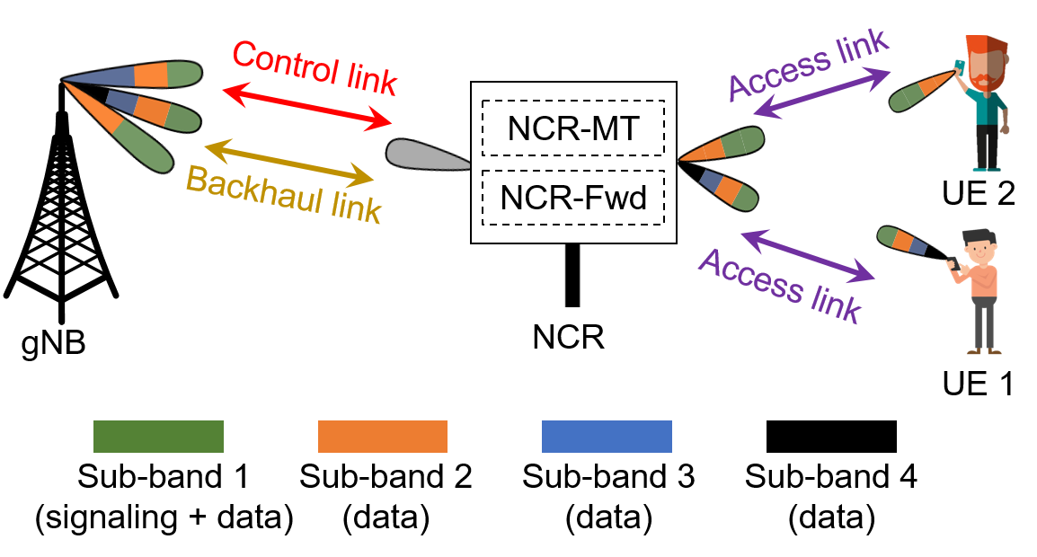
Figure 1: NCR supporting subband operation.

A challenge that needs to be overcome to enable subband signaling operation with repeater nodes, e.g., NCRs and RISs, is that the array radiation pattern can be frequency dependent and, therefore, beam misalignment can occur due to the effect of beam squinting. Thus, reusing the transmitter parameters, e.g., beamforming filters, defined for a given subband in other subbands may lead to performance degradation. Beam squinting has been the main subject of some articles in the literature in different contexts. In [11], the authors studied the impact of beam squinting in uniform linear array (ULA) with analog beamforming. In order to reduce the impact of beam squint in a wideband scenario, the authors suggested a codebook design to enforce a minimum array gain in the whole bandwidth.

Beam squint for wideband hybrid beamforming was considered in [12, 13, 14, 15, 16]. In [15], analog and digital precoders/combiners were designed to maximize spectral efficiency. In [12], the authors proposed two beamforming techniques to combat beam squinting where analog and digital precoders/combiners were designed. Firstly, the authors proposed a virtual sub-array architecture that performs a beam broadening that provides a more uniform gain over the operating frequency range. The other solution is based on the addition of a few true-time-delay lines to compensate for differences in time delays among different antennas. True-time-delay lines were also considered in [13, 14, 16] associated with analog phase shifts in order to make phase shifts frequency dependent. Although the use of true-time-delay lines improves performance by mitigating beam squinting, they increase energy consumption and hardware cost compared to conventional designs.

Beam squinting was also studied for RIS-assisted networks [17, 18]. In [17], the authors analyzed the impact of beam squinting in near and far fields. To mitigate beam squinting, the authors proposed a delay adjustable metasurface architecture that is equivalent to the use of true-time-delay lines in phased antenna arrays. Therefore, signals reflected by different RIS elements are submitted to adjustable delays in order to deal with the beam gain loss caused by beam squinting. In [18], the authors focused on channel estimation methods for wideband RIS, and proposed a method for the frequency domain channel response estimation based on cross-entropy theory.

In this paper, we study the problem of beam squinting in NCR-assisted networks. Although our proposed method can be applied to general multiple input multiple output (MIMO) scenarios, NCRs can be deployed in crowded areas where the distances to the terminals are not high. Thus, UEs are not necessarily aligned to the antenna boresight of NCR panels, which increases the beam squinting effect. Motivated by this, we characterize the beam squinting phenomenon in the context of subband operation and propose a beam squinting compensation method to enable the aforementioned subband operation illustrated in Fig. 1. Then, we present a system-level performance evaluation where we show the impact of beam squint in the aforementioned scenario. Beam squinting leads to both main lobe misalignment in the radiation pattern as well as higher interference in the system, which decreases signal to interference-plus-noise ratio (SINR). Furthermore, we show that our proposed compensation method is capable of keeping a similar system performance in terms of throughput and SINR for different carrier frequency displacements by avoiding the undesired effects of beam squinting.

Our work is different from those in the literature because previous works [11, 12, 13, 14, 15, 16, 13, 14, 16, 17, 18] in general had the objective of increasing the operation bandwidth of the antenna arrays by mitigating beam squinting. On the other hand, our objective is to reduce the beam squinting in order to transmit in a second subband based on the collected information, e.g., channel state information (CSI), and transmission parameters, e.g., precoders, collected/defined from/to a first subband. Moreover, previous works in general focused on simple evaluation scenarios involving few network nodes and, thus, are not capable of showing the achievable gains of their proposals from a system-level perspective. Finally, our proposed beam squinting compensation method has not been presented before.

The present work is organized as follows. First, in Section II, we provide a high-level discussion on the problem of beam squinting. Then, in Section III, we present a generic model for antenna array and discuss the array beam pattern for different frequencies. In Section IV, we analytically show the phase deviation problem and present our proposed solution. Section V presents a performance evaluation of our proposed method based on simulations. Finally, Section VI presents the conclusions of this work.

II Beam squinting: high-level characterization

Together with the antenna element radiation pattern, the antenna array geometry is one of the defining characteristics of the performance of a system employing MIMO antennas. When designing a MIMO system, regular/uniform geometries are usually applied (despite not mandatory) so that most 5G communication system assume the usage of standard linear arrays or standard rectangular arrays. By standard herein, one means that the antenna element spacing $d$ in the antenna arrays is normally set to $\frac{\lambda_{c}}{2}$, where $\lambda_{c}$ is the wavelength of the central carrier frequency $f_{c}$ of the system being designed. With such spacing, signals impinging as a planar wavefront on the antenna arrays are spatially sampled in an optimum way according to Nyquist’s theorem. As a consequence, several important properties, such as beam orthogonality, can be exploited by the MIMO systems to spatially filter signals, to reinforce components of interest and/or suppress interfering ones.

These assumptions are valid for narrow band systems in which the system bandwidth $B$ around $f_{c}$ is very small compared to the carrier frequency itself, i.e., $f_{c}\gg B$. In this case, frequencies $f=f_{c}\pm\frac{B}{2}$ lead to wavelengths $\lambda\approx\lambda_{c}$. However, with the advent of mmWave and possible use of sub-THz in 6G, broadband systems are expected to operate with much larger bandwidths than their predecessors and its contemporaneous sub-$6\text{\,}\mathrm{G}\mathrm{H}\mathrm{z}$ version. In this sense, systems designed for a center carrier frequency $f_{c}=f_{1}$, i.e., with antenna arrays designed considering $\lambda_{c}=\lambda_{1}$, but operating with multiple subbands, such as 5G NR, might suffer from spatial aliasing. This may occur because, for a subband at frequency $f_{2}=f_{1}+\Delta f,\Delta f>0$, and having a wavelength $\lambda_{2}<\lambda_{1}$, the antenna element spacing will be perceived at the frequency $f_{2}$ as an antenna array designed with a suboptimal antenna element spacing $\frac{\lambda_{1}}{2}$ larger than the ideal one $\frac{\lambda_{2}}{2}$ for $f_{2}$. In the case of $\Delta f<0$, the same effect would take place but the antenna element spacing would be smaller than the ideal one.

If the antenna element spacing is larger than the ideal one (i.e., $\frac{\lambda_{i}}{2}>\frac{\lambda_{c}}{2}$ for frequency $f_{i}$), the expected spatial aliasing effect is a “compression” in the beam space generating narrowed grating lobes. On the other hand, if the antenna element spacing is smaller ($\frac{\lambda_{i}}{2}<\frac{\lambda_{c}}{2}$) than the ideal one, grating lobes still appear, however as “widened” beams [19, Sec. 2.4.1.2]. In both cases, for a certain angular position associated with a beam at the center carrier frequency $f_{1}$, there will be angular shifts for the actual beam observed at frequency $f_{2}$. This change in how spatial signals and beams are viewed by the antenna array depending on the frequency (or subband) is also termed beam squinting. Notice that, often the beam associated with a UE might represent the only angular information about that UE. Therefore, angular shifts of beams may strongly affect the link quality of the UEs associated with those beams.

In Fig. 2, we illustrate the beam squinting phenomenon for a transmitter equipped with a 256-linear antenna array with elements spaced by half wavelength assuming a center frequency $f_{c}=28$ GHz. In this figure, we show the antenna array radiation pattern for a beam designed (with a proper set of phase shifts) for the operating frequency $f_{c}$ (solid blue curve), and the array radiation patterns for the same phase shift configuration but at frequencies $f_{c}+\Delta f$ and $f_{c}-\Delta f$ (dashed-red and dotted-green curves, respectively) assuming $\Delta f=1\text{ GHz}$. Figure 2 is composed of three subfigures, i.e., 2a, 2b and 2c, where a beam was designed at frequency $f_{c}$ for an impinging wavefront direction close to the antenna boresight, another intermediate direction, and an impinging wavefront direction close to the antenna array endfire, respectively.

From Fig. 2, it is clear that the beam squinting, i.e., the beam deviation, increases with $\Delta f$ and the angle which the beam was designed to point to relative to the antenna array boresight. For example, while the beam deviation for a beam pointing closely to the array boresight at $f_{c}+\Delta f$ was $0.57^{\text{o}}$, the beam deviation changes to $5.34^{\text{o}}$ for a beam at the same frequency pointing to an angle close to the array endfire. In the context of NCRs, this can be an issue since NCRs are usually deployed close to the UEs and so they are not necessarily aligned to the array boresight direction, being served by beams close to the array endfire.

Another aspect that can be confirmed in Fig. 2 is the beam widening and compression when the operating frequency is lower than or greater than $f_{c}$, respectively. For example, in Fig. 2c, the half power beamwidth (HPBW) for the beams at frequencies 28 GHz, (28 + 1) GHz and (28 - 1) GHz are $1.33^{\text{o}}$, $1.11^{\text{o}}$ and $1.99^{\text{o}}$, respectively.

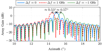
(a) Pointing direction close to the antenna boresight.

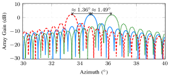
(b) Intermediate pointing direction.

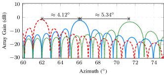
(c) Pointing direction close to the antenna endfire.

Figure 2: Beam squinting representation considering a ULA with 256 elements placed on the $y$-axis at $f_{c}=28$ GHz and a frequency offset $\Delta f=\pm 1$ GHz and beams pointing toward different directions.

In Fig. 3, we present another perspective of the beam squinting problem assuming the same antenna configuration as in Fig. 2. However, the figure presents the array gain in dB versus the frequency deviation, $\Delta f$, assuming different beams whose main lobe points to azimuths $15^{\text{o}}$ (blue curve), $35^{\text{o}}$ (red curve) and $66^{\text{o}}$ (green curve) which represent examples of beams pointing to boresight, an intermediate direction and endfire of the antenna array, respectively. From this figure we observe in a more direct way the impact of the frequency deviation on the array gain loss due to the beam squinting phenomenon. Furthermore, as the absolute value of frequency deviation increases, the array gain decreases differently depending on the main lobe direction of the beams. The array gain of beams close to the boresight (blue curve, for example) requires a higher frequency deviation in order to present a significant loss (due to beam squinting). However, beams near the endfire of the antenna array (green curve, for example) are more sensitive to the frequency deviation.

Beam squinting was also discussed analytically in [20], where the authors derived an equation that shows the beam squinting for a linear array with equally spaced antenna elements assuming ideal phase shifters. The beam squinting was defined as the change in the beam main lobe direction, $\Delta\theta$, in terms of the original beam main lobe direction, $\theta_{1}$, the original operation frequency, $f_{1}$, and the frequency deviation, $\Delta f$. This equation is given by

$$\Delta\theta=-\tan\mathopen{}\mathclose{{}\left(\theta_{1}}\right)\frac{\Delta f}{f_{1}}.$$ (1)

By analyzing (1), one can reach the same conclusions as we described for Fig. 2. The beam misalignment due to beam squinting can, for example, cause reduced received power at UEs. This is specially critical as the number of antenna array elements increases and, therefore, beams become more and more narrow.

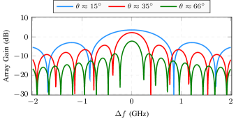
Figure 3: Beam squinting representation considering a ULA with 256 elements placed on the $y$-axis at $f_{c}=28$ GHz.

III System Model

In this section, we assume a generic antenna array where a filter (or beamformer) is applied. Then, the array beam response is presented when two different frequencies are assumed.

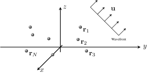
Figure 4: General antenna array representation.

Consider an antenna array with $N$ elements placed at positions $\mathbf{r}_{i}$, for $n\in\{1,\cdots,N\}$, as shown in Fig. 4. Each element of the array has a radiation pattern given by $a(\mathbf{u})$, with $\mathbf{u}$ denoting the direction unit vector pointing towards the azimuth $\theta\in(-180^{\circ},180^{\circ})$ and zenith $\phi\in(0^{\circ},180^{\circ})$, i.e.,

$$\mathbf{u}={\begin{bmatrix}\sin(\phi)\cos(\theta)&\sin(\phi)\sin(\theta)&\cos(\phi)\end{bmatrix}}^{\mathrm{T}}.$$ (2)

Furthermore, consider that a planar wavefront departs toward the direction $\mathbf{u}$ at frequency $f_{c}=f_{1}$. In this case, the array response can be written as

$$\mathbf{v}(\mathbf{u})=a(\mathbf{u})\cdot{\begin{bmatrix}\psi_{1}&\psi_{2}&\cdots&\psi_{N}\end{bmatrix}}^{\mathrm{T}},$$ (3)

where $\psi_{n}=\exp\mathopen{}\mathclose{{}\left(j\frac{2\pi f_{1}}{c}{\mathbf{u}}^{\mathrm{T}}\mathbf{r}_{n}}\right)$ for $n\in\{1,\cdots,N\}$.

In order to shape and steer the beam toward an arbitrary direction $\mathbf{u}_{t}$, the transmitter must apply a filter (or beamformer), which consists of a set of weighting factors applied on each element. A general filter can be defined as

$$\mathbf{w}_{1}={\begin{bmatrix}g_{1}\exp(j\omega_{1})&g_{2}\exp(j\omega_{2})&\cdots&g_{N}\exp(j\omega_{N})\end{bmatrix}}^{\mathrm{T}},$$ (4)

where $g_{n}$ and $\omega_{n}$, for $n\in\{1,\cdots,N\}$, represent the magnitude and phase of each weight, respectively.

The beam pattern of the array combined with the filter is given by

$$B_{1}(\mathbf{u}) ={\mathbf{w}}^{\mathrm{T}}_{1}\mathbf{v}(\mathbf{u})$$

$$=a(\mathbf{u})\sum_{n=1}^{N}g_{n}\exp\mathopen{}\mathclose{{}\left(j\frac{2\pi f_{1}}{c}{\mathbf{u}}^{\mathrm{T}}\mathbf{r}_{n}+j\omega_{n}}\right).$$ (5)

The direction $\mathbf{u}^{\star}$ where the array presents its maximum gain is given by

$$\mathbf{u}^{\star}=\underset{\mathbf{u}}{\arg\max}\mathopen{}\mathclose{{}\left\{\mathopen{}\mathclose{{}\left|B_{1}(\mathbf{u})}\right|}\right\}.$$ (6)

Consider that the same filter $\mathbf{w}_{1}$ is used to beamform the array response, but operating at a frequency $f_{2}=f_{1}+\Delta f$. As briefly addressed in Section II, the frequency deviation implies at a direction change. Replacing the frequency $f_{1}$ in (III) by $f_{2}$, the beam pattern $B_{2}(\mathbf{u})$ is given by

$$B_{2}(\mathbf{u}) =a(\mathbf{u})\sum_{n=1}^{N}g_{n}\exp\mathopen{}\mathclose{{}\left(j\frac{2\pi(f_{1}+\Delta f)}{c}{\mathbf{u}}^{\mathrm{T}}\mathbf{r}_{n}+j\omega_{n}}\right)$$

$$=a(\mathbf{u})\sum_{n=1}^{N}g_{n}\exp\mathopen{}\mathclose{{}\left(j\frac{2\pi f_{1}}{c}{\mathbf{u}}^{\mathrm{T}}\mathbf{r}_{n}+j\omega_{n}}\right)d_{n}(\mathbf{u}),$$ (7)

where

$$d_{n}(\mathbf{u})=\exp\mathopen{}\mathclose{{}\left(j\frac{2\pi\Delta f}{c}{\mathbf{u}}^{\mathrm{T}}\mathbf{r}_{n}}\right)$$ (8)

denotes the phase deviation at each antenna element $n$.

IV Problem Definition and Proposed Solution

Based on the antenna model and array beam pattern presented for two different frequencies, i.e., $f_{1}$ and $f_{2}$, in Section III, in this section, we firstly present the phase deviation that characterizes the beam squinting. In order to cope with this, we then propose a filter to be applied at frequency $f_{2}$ to compensate for this phase deviation. Then, we particularize the proposed phase compensation for different array configurations. Finally, we discuss the main limitations of our proposal and also present a path loss compensation that can be used together with our phase compensation proposal.

IV-A Phase Deviation and Compensation

Comparing $B_{1}(\mathbf{u})$ in (III) and $B_{2}(\mathbf{u})$ in (III), note that $B_{2}(\mathbf{u})$ presents a $d_{n}(\mathbf{u})$ at each antenna element $n$. In order to compensate for the deviation $d_{i}$, the filter $\mathbf{w}_{2}$ used at frequency $f_{2}$ should be properly designed as

$$\mathbf{w}_{2}=\mathbf{w}_{1}\odot\mathbf{c},$$ (9)

where the operator $\odot$ denotes the Hadamard product and $\mathbf{c}$ is the compensation vector designed to cancel the effect of the deviation.

Ideally, to completely cancel the effect of the deviation, each element $c_{n}$ of $\mathbf{c}$ associated with the $n$-th antenna element should be equal to $d^{*}_{n}(\mathbf{u})$, i.e., $c_{n}(\mathbf{u})=d^{*}_{n}(\mathbf{u})$. However, this ideal canceling is impossible, since it would require that the filter $\mathbf{w}_{2}$ was adapted at each wavefront direction. Besides that, the filter $\mathbf{w}_{1}$ is normally designed to be used when transmitting (or receiving) data to or from another device that is placed in a certain direction $\mathbf{u}^{\star}$ or in its vicinity. This direction is determined, e.g., by the maximum array response as in (6) and its vicinity depends on the beam width.

Considering the prior discussion and the assumption of knowing $\mathbf{u}^{\star}$ obtained in (6), we propose to define and apply a compensation vector $\mathbf{c}$ given by

$$\mathbf{c}={\begin{bmatrix}\psi_{1}^{\star}&\psi_{2}^{\star}&\cdots&\psi_{N}^{\star}\end{bmatrix}}^{\mathrm{T}}$$ (10)

where $\psi_{n}^{\star}=\exp\mathopen{}\mathclose{{}\left(-j\frac{2\pi\Delta f}{c}{(\mathbf{u}^{\star})}^{\mathrm{T}}\mathbf{r}_{n}}\right)$, for $n\in\{1,\cdots,N\}$, to cope with the beam misalignment suffered by a beam designed to operate at frequency $f_{1}$ but operating at a frequency $f_{2}=f_{1}+\Delta f$.

This compensation method has the following advantages:

1. The direction $\mathbf{u}^{\star}$ can be calculated once for each antenna array model, and does not depend on the antenna array placement or mechanical tilts, as long as the referential remains the same (e.g., antenna boresight);

2. Since the compensation vector $\mathbf{c}$ only applies phase shifts, it can be used with analog, digital and hybrid beamformers;

3. If the device uses a codebook at $f_{1}$, another codebook to be used at $f_{2}$ can be computed once and stored or even embedded at the devices during manufacturing.

Notice that due to the usage of massive MIMO antenna arrays in 5G and beyond, the width of the beams in these systems can be very narrow and even a small angular misalignment might have a considerable impact on the system performance. This reinforces the importance of the compensation method proposed in our work.

Besides that, in beam-based 5G and next generation systems, beam directions are often constrained to a limited number of discrete angular values, namely these of the beamforming codebook. Thus, since usually the angular positions of the UEs are considered to be the same as that of the beam selected for them for transmission and/or reception, this relatively coarse angular resolution can lead to additional angular deviations with respect to the actual angular position of the UEs. In other words, inherently the angular position of the UEs might not be known as precisely as it is assumed here, which may increase harming effects caused by angular misalignment induced by beam squinting. These facts strengthen even more the relevance of our proposed method, which mitigates such harming effects.

IV-B Phase Shift Compensation for an ULA

Consider an ULA with $N$ elements placed along the $y$-axis, spaced by $\frac{\lambda_{c}}{2}$, where $\lambda_{c}$ is the wavelength associated to frequency $f_{c}=f_{1}$. Moreover, consider that the array boresight is pointing towards the positive $x$-axis, i.e., boresight at $\theta=0^{\text{\textdegree}}$, as depicted in Fig. 5.

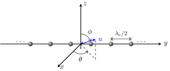
Figure 5: Representation of an ULA placed along the $x$-axis.

The position of the $n$-th element of this ULA is given by

$$\mathbf{r}_{n}={\begin{bmatrix}0&\mathopen{}\mathclose{{}\left(n-\dfrac{N+1}{2}}\right)\dfrac{\lambda_{c}}{2}&0\end{bmatrix}}^{\mathrm{T}}.$$ (11)

Each element of the compensation vector $\mathbf{c}$ is given by

$$c_{n} =\exp\mathopen{}\mathclose{{}\left(-j\frac{2\pi\Delta f}{c}\mathopen{}\mathclose{{}\left(n-\frac{N+1}{2}}\right)\frac{\lambda_{c}}{2}\sin(\phi^{\star})\sin(\theta^{\star})}\right)$$

$$=\exp\mathopen{}\mathclose{{}\left(-j\frac{\pi\Delta f}{f_{1}}n\sin(\phi^{\star})\sin(\theta^{\star})}\right)\times$$

$$\hskip 10.76385pt\exp\mathopen{}\mathclose{{}\left(j\frac{\pi\Delta f}{f_{1}}\frac{N+1}{2}\sin(\phi^{\star})\sin(\theta^{\star})}\right),$$ (12)

where $\theta^{\star}$ and $\phi^{\star}$ correspond to the azimuth and zenith where the ULA achieves its maximum gain. Notice that the second exponential does not depend on the antenna element, i.e., the same phase shift is applied to all elements. It is well known that this shift does not affect the direction of the beam, therefore it can be ignored.

The ULA does not have resolution along $\phi$, i.e., the beam pattern along $\phi$ is the same as the element pattern. Moreover, the maximum gain of an antenna element is usually designed to point towards the boresight of the array, implying at $\phi^{\star}=90^{\circ}$ for every adopted filter. Therefore, the $i$-th element of the compensation vector is given by

$$c_{n}=\exp\mathopen{}\mathclose{{}\left(-j\frac{\pi\Delta f}{f_{1}}n\sin(\theta^{\star})}\right),\,\forall n.$$ (13)

Figure 6 illustrates the same example presented in Fig. 2b, but now including two new curves. The new curves are related to $\Delta f=\pm 1\text{ GHz}$, while considering the proposed compensation presented in (13). We observe that the main lobes of $\Delta f=0\text{ GHz}$ and $\Delta f=\pm 1\text{ GHz}$ (compensated) match, which means that our proposal is able to mitigate the beam squinting even for a high value of $\Delta f$. Assuming that a given UE is approximately aligned in the direction with azimuth $34.7^{\circ}$, at the original carrier frequency, i.e., $\Delta f=0$, this UE experiences maximum array gain (peak value of the solid-blue curve). However, if the same precoder or transmit filter is applied at a different frequency with $\Delta f=1\text{ GHz}$, the maximum array gain is pointing towards azimuth direction of approximately $33.6^{\circ}$ (dashed-red curve). Thus, the aforementioned UE would now experience an array gain much lower than the original designed one. The compensation is capable of keeping the maximum array gain towards the original UE direction even at a different frequency. Although our compensation method focuses on aligning the main lobe of the radiation patterns for $\Delta f=0\text{ GHz}$ and $\Delta f\neq 0\text{ GHz}$, an added benefit is that nulls near the main lobe also match for both operating frequencies as it can be seen in  Fig. 6. Thus, our method not only guarantees that the maximum gain towards a specific receiver is kept, but also avoids interference to other receivers resulting from beam squint effect.

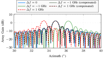
Figure 6: Illustration of beam squinting compensation for a ULA with 256 elements and $f_{c}=28\text{ GHz}$.

IV-C Phase Shift Compensation for a URA

Consider an URA with $N_{r}\times N_{c}$ elements placed along the $yz$-plane, spaced by $\frac{\lambda_{c}}{2}$. Moreover, the array boresight is pointing towards the positive $x$-axis, as depicted in Fig. 7.

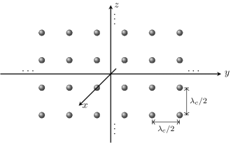
Figure 7: Representation of an URA placed along the yz-plane, pointing towards the $x$-axis.

Following the same steps as for the ULA, the position of the $n$-th element of this ULA is given by

$$\mathbf{r}_{n}={\begin{bmatrix}0&\mathopen{}\mathclose{{}\left(n_{r}-\dfrac{N_{r}+1}{2}}\right)\dfrac{\lambda_{c}}{2}&\mathopen{}\mathclose{{}\left(n_{c}-\dfrac{N_{c}+1}{2}}\right)\dfrac{\lambda_{c}}{2}\end{bmatrix}}^{\mathrm{T}},$$ (14)

where $n_{r}\in\{1,\cdots,N_{r}\}$ and $n_{c}\in\{1,\cdots,N_{c}\}$ denote the index of the row ($z$-axis) and column ($y$-axis) of the URA, respectively.

Considering the element positioning in (14) and removing the antenna independent phase shift, the same as in (IV-B) and (13) for the ULA, each element of the compensation vector $\mathbf{c}$ is given by

$$c_{n}=\exp\mathopen{}\mathclose{{}\left(-j\frac{\pi\Delta f}{f_{1}}\mathopen{}\mathclose{{}\left(n_{r}\sin(\phi^{\star})\sin(\theta^{\star})+n_{c}\cos(\phi^{\star})}\right)}\right).$$ (15)

Figure 8 illustrates the proposed beam squinting compensation for a $32\times 32$ URA. This figure presents the gain of this URA for five different cases. Three different values of $\Delta f$ are evaluated, i.e., $\Delta f=0\text{ GHz}$ and $\Delta f=\pm 1\text{ GHz}$. For $\Delta f=\pm 1\text{ GHz}$, two possibilities are considered, i.e., with and without the proposed beam squinting compensation. Comparing these five cases we can conclude that our proposal is able to compensate for the beam squinting that occurs for $\Delta f=\pm 1\text{ GHz}$. The advantage in terms of interference avoidance as discussed for Fig. 6 can also be observed in this case.

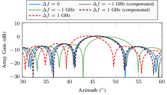
(a) Azimuth.

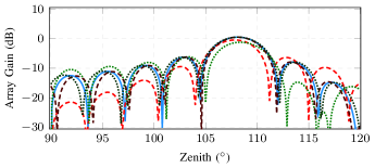
(b) Zenith.

Figure 8: Illustration of beam squinting compensation for a URA $32\times 32$ and $f_{c}=28\text{ GHz}$.

IV-D Limitations of the Proposed Phase Compensation Method

As observed in Figs. 6 and 8, the proposed solution successfully compensates for the beam squinting effect caused by frequency displacement. However, if the filter $\mathbf{w}$ yields an array response with main lobes pointing towards more than one direction, the solution proposed in the previous section may fail. This case may occur when the beam is steered close to the array endfire.

As an example, consider a ULA with 64 elements disposed along the $y$-axis and a filter $\mathbf{w}$ equal to the column of the DFT codebook that steers the beam closest to the array endfire. When applying our proposed compensation, the array response is compensated in only one direction, as depicted in Fig. 9.

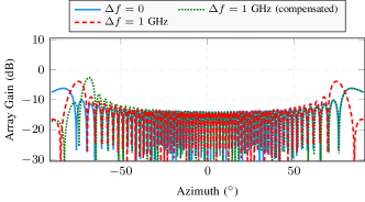
Figure 9: Array gain of a ULA with $64$ elements with beam steering close to the array endfire.

Notice, in Fig. 9, that the chosen filter fits to serve devices placed at an azimuth direction around $[-90^{\circ},-80^{\circ}]$ or $[80^{\circ},90^{\circ}]$. As already discussed, the proposed solution needs prior knowledge of which direction $\mathbf{w}$ steers the array to in order to properly compensate it. In this example, only the positive azimuth direction is compensated, which yields to an inappropriate antenna gain if the served device is placed at the negative azimuth.

In order to address this issue, when the value $\mathbf{w}$ leads to more than one beam direction, the transmitter should make use of the device’s direction, in order to properly compensate for the beam squinting effect. The device’s direction can be estimated using, for example, the beam tracking procedure, or the synchronization signal block (SSB) measurements. Therefore, considering the case where $\mathbf{w}$ beamforms the array towards $D$ different directions $\mathbf{u}^{\star}_{i}$ for $i\in\{1,\ldots,D\}$, and the served device’s estimated direction is $\tilde{\mathbf{u}}$, the proposed solution should compensate for the beam squinting towards the direction $\mathbf{u}^{\star}=\mathbf{u}^{\star}_{i^{\dagger}}$

$$i^{\dagger}=\underset{i}{\arg\min}\mathopen{}\mathclose{{}\left\{\mathopen{}\mathclose{{}\left\|\mathbf{u}^{\star}_{i}-\tilde{\mathbf{u}}}\right\|}\right\}.$$ (16)

On the other hand, the filters are normally designed to address devices upon a single direction, and are taken from a predefined set, like the aforementioned example, where $\mathbf{w}$ was taken from the discrete fourier transform (DFT) codebook. Moreover, the array is normally designed to irradiate most of its energy to its front. Therefore, in such use cases, the only situation where $\mathbf{w}$ beamforms the array response to more than one direction is when $\mathbf{w}$ steers the response close to the array endfires, as depicted in Fig. 9. In this situation the strategy proposed in (16) can be quite simplified. When the array is an ULA and the DFT codebook is employed, just one filter (one codebook entry) has ambiguous directions. In order to disambiguate it, the transmitter should estimate whether the azimuth of the served device with respect to the array boresight is greater than 0. If an URA is considered, some filters of the codebook need disambiguation, due to azimuth and zenith endfires. In this case, besides the azimuth, the transmitter must estimate whether the zenith is greater than $90^{\circ}$.

IV-E Path Loss Compensation

Besides the phase compensation discussed in this section, the use of different frequencies can also impact on long-term channel characteristics, e.g., path loss. Thus, assume a generic path loss model (in dB)

$$L_{k}=a+b\cdot\log_{10}\mathopen{}\mathclose{{}\left(d_{3D}}\right)+c\cdot\log_{10}\mathopen{}\mathclose{{}\left(f_{k}}\right),$$ (17)

where $a$, $b$ and $c$ are constants of the model, $d_{3D}$ is the distance between the transmitter and receiver, and $f_{k}$ is the considered frequency. By assuming two different frequencies, $f_{1}$ and $f_{2}$ where $f_{2}=f_{1}+\Delta f$ and $f_{2}>f_{1}$, we can show that the positive difference in path loss is

$$L_{2}-L_{1}=c\cdot\log 10\mathopen{}\mathclose{{}\left(1+\frac{\Delta f}{f_{1}}}\right).$$ (18)

For $f_{1}$ in the order of tens of GHz (mmWave) and $\Delta f$ in the order of hundreds of MHz, $L_{2}-L_{1}$ will be small. For example, considering $f_{1}=$28\text{\,}\mathrm{G}\mathrm{H}\mathrm{z}$$, for $L_{2}-L_{1}\geq$0.3\text{\,}\mathrm{d}\mathrm{B}$$, then $\Delta f\geq$1\text{\,}\mathrm{G}\mathrm{H}\mathrm{z}$$. Thus, for $f_{k}$ in mmWave, as in 5G, we do not expect an important variation of the path loss in a bandwidth of a few hundreds of MHz.

V Performance Evaluation: Case Study with 5G/NR and NCRs

Although our proposed beam compensation method applies to general multiple-antenna transmitters, e.g., base stations (BSs), RISs and NCRs, in this section, we present the simulation results for NCR-assisted networks to evaluate the impact of our beam squinting compensation proposal in the NCR subband operation. Here, we consider system-level analysis where the effect on beam squinting on both the useful and interfering signals can be well studied. In our performance evaluation, we consider the downlink direction and that the beam squinting compensation method is applied at both gNB and NCR nodes. NCRs were chosen in our analysis because, different from RISs, have been standardized by 3GPP and have shown better performance when compared to RISs [3]. Another motivation for this case study is that NCRs may be deployed in crowded areas where their distance to the UEs may be not high and the UEs are not necessarily aligned to the array boresight direction and they can be served by beams close to the antenna array endfire. Thus, depending on the NCR deployment, it is expected for the beam squinting phenomenon to have an important impact on NCR subband operation.

The details concerning the considered simulation modeling are presented in Section V-A and the results are discussed in Section V-B.

V-A Simulation Scenario, NCR Modeling and Parameters

Figure 10 illustrates the adopted scenario. A simplified version of the Madrid grid [21] is considered. In this scenario, there are $9$ square blocks, with dimension of $120\text{\,}\mathrm{m}$ $\times$ $120\text{\,}\mathrm{m}$ surrounded by $3\text{\,}\mathrm{m}\text{/}$ wide sidewalks and separated of each other by $14\text{\,}\mathrm{m}$ wide streets. The UEs are randomly placed in the sidewalks of a crowded street. They are allowed to cross the street only in the intersections. The closest gNB is deployed some blocks away. An NCR, controlled by the gNB, is deployed in the street where the UEs are located in order to improve the system coverage in that area.

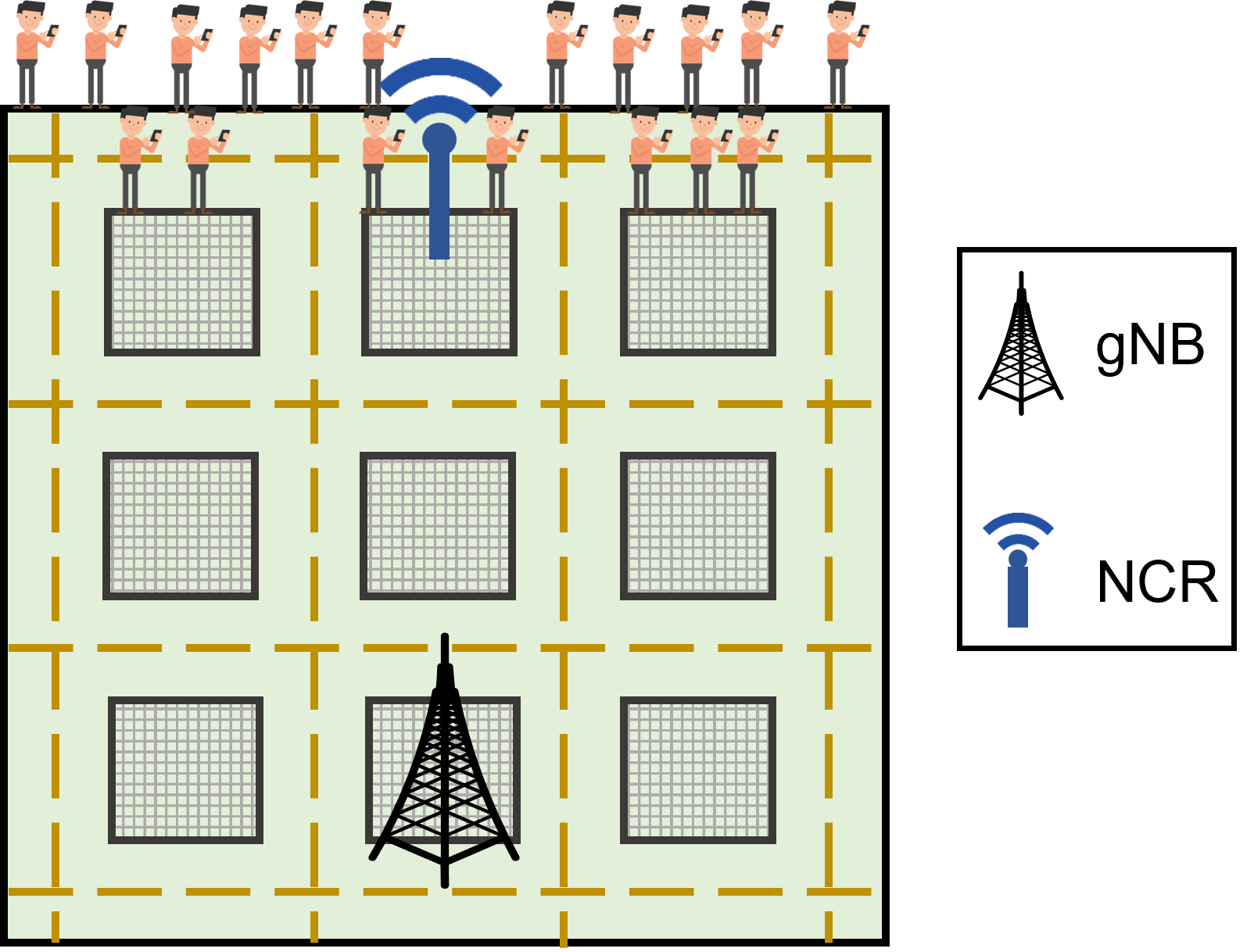
Figure 10: Considered scenario.

Regarding the NCR, at each transmission time interval (TTI) $t$, it applies a fixed gain of 60 dB to the signal received at each resource block (RB). If the signal output power of the NCR with fixed gain is higher than the maximum NCR output power, the gain $g_{k}$ at RB $k$ will be given as

$$g_{k}(t)=\frac{p^{\text{NCR}}_{k}}{\sigma_{k}^{2}+\gamma_{k}(t)\cdot p_{\mathrm{tx},k}(t)},$$ (19)

where $\sigma_{k}$ is the noise power at the bandwidth of RB $k$; $\gamma_{k}(t)=|\textbf{d}_{k}(t)\textbf{Q}_{k}(t)\textbf{w}_{k}(t)|^{2}$ denotes the combined effect of the channel $\textbf{Q}_{k}$ after the transmission filter at the gNB, $\textbf{w}_{k}$, and the reception filter at NCR, $\textbf{d}_{k}$, applied to a signal transmitted with transmit power $p_{\mathrm{tx},k}$; and $p^{NCR}_{k}$ is the output power of the NCR, which is constant, since it is considered equal power allocation (EPA) among the RBs.

All links between the nodes in the system, i.e., UEs, NCR and gNB, are modeled according to the 3GPP channel model specifications [22, 23]. It is a spatially and temporally consistent model that considers a distance-dependent path-loss, a lognormal shadowing component and small-scale fading.

Concerning the UEs’ signal strength measurements at $f_{1}$, the gNB periodically performs beam sweeping with SSBs and channel state information reference signal (CSI-RS) [24]. Some of the SSBs/CSI-RSs are amplified and forwarded by the NCR, while others arrive directly from the gNB to the UEs. For each received SSB/CSI-RS, a UE measures its reference signal received power (RSRP), which is the linear average over the power contributions (in Watts) of the resource element confined within a transmitted SSB/CSI-RS [25]. The measured RSRPs are then reported to the gNB. Based on the received measurement reports, the gNB chooses whether the UE should be served directly or through the NCR. Similarly, the NCR also measures and reports to the gNB the RSRP of the received SSBs/CSI-RSs in order to allow the gNB to perform link adaptation of the control and backhaul links (see Fig. 1).

The links between gNB and NCR, i.e., control and backhaul, are stable and planned during network deployment. On the other hand, the links between UEs-gNB and UEs-NCR vary more frequently due to the UEs mobility. Thus, the beam sweeping of beams related to control and backhaul links are performed less frequently than the beam sweeping of beams related to access links.

The system parameters are aligned with NR 3GPP specifications series $38$ Release $17$. The simulations are conducted at $28\text{\,}\mathrm{GHz}\text{/}$. Four different values of $\Delta f$ are considered: $0\text{\,}\mathrm{M}\mathrm{H}\mathrm{z}$, $100\text{\,}\mathrm{M}\mathrm{H}\mathrm{z}$, $500\text{\,}\mathrm{M}\mathrm{H}\mathrm{z}$ and $1\text{\,}\mathrm{G}\mathrm{H}\mathrm{z}$. An RB, i.e., the minimum scheduling unit in the frequency domain, consists of $12$ consecutive subcarriers spaced $60\text{\,}\mathrm{k}\mathrm{H}\mathrm{z}$ of each other. Thus, $66$ RBs are considered. Moreover, we consider an additive white gaussian noise (AWGN) power per subcarrier of $-174\text{\,}\mathrm{d}\mathrm{B}\mathrm{m}$, noise figure of $9\text{\,}\mathrm{d}\mathrm{B}$ and shadow standard deviation of $4\text{\,}\mathrm{d}\mathrm{B}$. In the time domain, a slot is the minimum scheduling unit, consisting of $14$ orthogonal frequency division multiplexing (OFDM) symbols with total time duration of $0.25\text{\,}\mathrm{ms}\text{/}$.

Regarding resource scheduling, in the frequency domain, the round robin (RR) scheduler is adopted to schedule the RBs. The RR iteratively allocated the RBs, scheduling in a given RB the UE bearer waiting the longest time in the queue. The RR is chosen since it is a well-known scheduler enabling an interested reader to reproduce our performance evaluation. Besides, our main objective is not to find the scheduler that optimizes the system behavior, but rather compare the different configurations under the same conditions, i.e., using the same scheduler.

The channel quality indicator (CQI)/modulation and coding scheme (MCS) mapping curves standardized in [26] are used for link adaptation with a target block error rate (BLER) of $10\text{\,}\%$. It is also considered an outer loop strategy to avoid the increase of the BLER. According to this strategy, when a transmission error occurs, the estimated SINR used for the CQI/MCS mapping in the link adaptation is subtracted by a back-off value of $1\text{\,}\mathrm{d}\mathrm{B}$. On the other hand, when a transmission occurs without error, the estimated SINR has its value added by $0.1\text{\,}\mathrm{d}\mathrm{B}$.

In the considered scenario, there are $72$ UEs with traffic modeled as constant bit rate (CBR) flows with packet size equal to 4,096 bits and packet-inter-arrival time equal to four slots. Table V-A presents other parameters considered in the simulations.

In the following, the computational results are presented. For each value of $\Delta f$, three possibilities are evaluated:

• CP transmitted at $28\text{\,}\mathrm{G}\mathrm{H}\mathrm{z}$ and DP transmitted at $($$28\text{\,}\mathrm{G}\mathrm{H}\mathrm{z}$+$\Delta f)$ without compensation,

• CP transmitted at $28\text{\,}\mathrm{G}\mathrm{H}\mathrm{z}$ and DP transmitted at $($$28\text{\,}\mathrm{G}\mathrm{H}\mathrm{z}$+$\Delta f)$ with compensation, and,

• Both CP and DP transmitted at $($$28\text{\,}\mathrm{G}\mathrm{H}\mathrm{z}$+$\Delta f)$,

where, as already mentioned, CP performs the transmission of signaling related to measurements used for RRM, e.g., link adaptation, and DP performs UE data transmission.

Finally, three gNB antenna array configurations are evaluated: ULA with $64,128\text{ and }256$ antenna elements. It is important to highlight that 3GPP plans to study antenna arrays with more than 64 elements in Rel. 19. Three key performance indicators (KPIs) are considered: the SINR, the throughput and the MCS usage, all of them in the downlink (DL).

TABLE I: Entities characteristics.

Parameter	gNB	NCR	UE
Height	$25\text{\,}\mathrm{m}\text{/}$	$10\text{\,}\mathrm{m}\text{/}$	$1.5\text{\,}\mathrm{m}\text{/}$
Transmit power	$35\text{\,}\mathrm{d}\mathrm{B}\mathrm{m}$	$33\text{\,}\mathrm{d}\mathrm{B}\mathrm{m}$	$24\text{\,}\mathrm{d}\mathrm{B}\mathrm{m}$
Antenna element pattern	3GPP 3D [22]	3GPP 3D [22]	Omni
Max. antenna element gain	$8\text{\,}\mathrm{d}\mathrm{B}\mathrm{i}$	$8\text{\,}\mathrm{d}\mathrm{B}\mathrm{i}$	$0\text{\,}\mathrm{d}\mathrm{B}\mathrm{i}$
Speed	$0\text{\,}\mathrm{k}\mathrm{m}\mathrm{/}\mathrm{h}$	$0\text{\,}\mathrm{k}\mathrm{m}\mathrm{/}\mathrm{h}$	$3\text{\,}\mathrm{k}\mathrm{m}\mathrm{/}\mathrm{h}$

V-B Simulation Results

Figure 11 presents the cumulative distribution function (CDF) of the UEs’ DL throughput. First, we observe that when CP and DP are transmitted at the same frequency, i.e., blue solid curve ($\Delta f=0$) and dotted curves, the UEs experience similar throughput. However, comparing these cases, i.e., CP and DP transmitted at the same frequency (blue solid curve and dotted curves) with the cases where CP and DP are transmitted at different frequencies without compensation (solid curves), we observe that the UEs throughput decreases. The impact of beam squinting increases for higher values of $\Delta f$, as expected.

Comparing the cases with and without our compensation proposal, i.e., solid and dashed curves, respectively, we observe that with our proposal the UEs’ throughput is similar to the cases when CP and DP were transmitted at the same frequency. Then, we can conclude that our proposed method is able to overcome the beam squinting issue. Furthermore, comparing Figures 10a, 10b and 10c, we observe that the beam squinting problem becomes more dominant (solid curves moved to the left) when the number of antenna elements increases, i.e., when we consider narrower beams. However, in all cases, our proposal is well able to compensate for the beam squinting. In these figures, we can see that the percentage of UEs with throughput lower than 1 Mbps assuming $\Delta f=500\text{MHz}$ and no compensation are equal to 37%, 57% and 71% whereas these values decrease to 18%, 4% and 0.2% when our proposed compensation method is applied for ULA with 64, 128 and 256 elements, respectively.

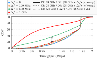
(a) ULA 64.

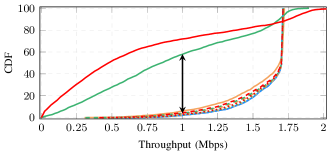
(b) ULA 128.

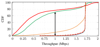
(c) ULA 256.

Figure 11: CDF of UE DL throughput.

Figure 12 presents another perspective of the one shown in Figure 11. In this figure, we show the throughput versus the frequency deviation assuming the cases without compensation, with compensation and the one where CP and DP are transmitted at the same frequency (no beam squinting). Figures 11a, 11b and 11c are for ULAs with 64, 128 and 256 antenna elements, respectively. Firstly, we can see that the cases without beam squinting, without compensation and with compensation presents a similar performance at the $90\%\text{-ile}$, which indicates that beam squint is not an issue for the UEs with high throughput, e.g., cell center UEs. However, beam squinting imposes an increasing performance loss as the frequency deviation increases for UEs in medium ($50\%\text{-ile}$) and poor ($10\%\text{-ile}$) channel conditions. Furthermore, we observe that the case with ULA 256 is the case where there is the highest performance loss when frequency deviation increases for medium and low percentiles illustrating the sensitivity of beam squinting for large antenna arrays. Our compensation method shows an almost constant performance with respect to the frequency deviation and very close to the case where CP and DP are transmitted at the same frequency. This shows the advantage of employing our method that is capable of keeping high throughput by compensating for the beam squinting effect especially for UEs in medium and poor channel conditions. This is particularly important because the main motivation for NCRs is to boost the performance of weak UEs.

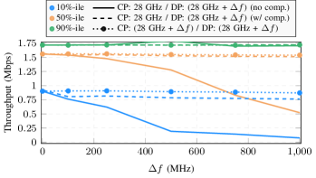
(a) ULA 64.

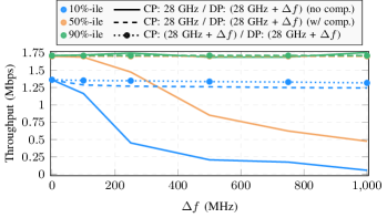
(b) ULA 128.

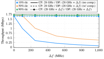
(c) ULA 256.

Figure 12: 10, 50 and 90%-ile of the UE DL throughput.

In Fig. 13, we present the SINR versus the frequency deviation assuming the cases without compensation, with compensation and the one where CP and DP are transmitted at the same frequency (no beam squinting). Figures 12a, 12b and 12c are for ULAs with 64, 128 and 256 antenna elements, respectively. As the SINRs are mapped to data rates through the link adaptation mechanism, Figs. 12 and 13 presents some similar aspects, but there are other important conclusions to highlight. The differences in SINR among 90%-ile, 50%-ile and 10%-ile are more prominent when compared with the same ones for throughput in the same percentiles in Fig. 12. The reason for that is the data rate saturation as the number of MCS schemes is finite, i.e., although the difference in SINR between 90%-ile and 50%-ile are more than 20 dB, this difference does not directly translate into a large difference in data rate.

In Fig. 13 we can also have another view on how system performance, in terms of SINR, degrades due to beam squinting with respect to frequency deviation and antenna array size. For the 90%-ile (UEs in best channel conditions), the SINR degradation due to beam squinting becomes more intense for frequency deviations of approximately 500 MHz, 200 MHz and 100 MHz for ULA with 64, 128 and 256 antenna elements, respectively. The sensitivity of the SINR of UEs in intermediate and worst channel conditions is higher with respect to frequency deviation compared to the 90%-ile case, as it can be seen in orange and blue curves. UEs with worst channel conditions are in general the ones far away from the gNB/NCR and also in the endfire of the antenna arrays where beam squinting is more significant, as previously explained.

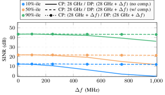
(a) ULA 64.

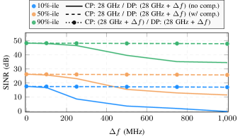
(b) ULA 128.

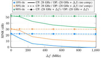
(c) ULA 256.

Figure 13: 10, 50 and 90%-ile of the UE DL SINR.

Fig. 14 presents the histogram of UEs’ MCS usage in DL for different values of $\Delta f$ considering a gNB with an ULA with 256 antenna elements. It compares three cases: i) CP and DP transmitted at the same frequency $(28\text{GHz}+\Delta f)$; ii) CP transmitted at $28\text{\,}\mathrm{G}\mathrm{H}\mathrm{z}$ and DP, at $(28\text{GHz}+\Delta f)$, without compensation; and iii) CP transmitted at $28\text{\,}\mathrm{G}\mathrm{H}\mathrm{z}$ and DP, at $(28\text{GHz}+\Delta f)$, with compensation.

As seen in Fig. 14, with our proposal, when transmitting CP at $28\text{\,}\mathrm{G}\mathrm{H}\mathrm{z}$ and DP at $(28\text{GHz}+\Delta f)$, the system achieves similar performance as when transmitting both CP and DP at the same frequency. On the other hand, without our proposal, the beam squinting deteriorates the system performance.

Notice in Figs. 13b and 13c that for $\Delta f=500\text{ MHz}$ and $\Delta f=1\text{ GHz}$, respectively, when CP is transmitted at $28\text{\,}\mathrm{G}\mathrm{H}\mathrm{z}$ and DP at $(28\text{ GHz}+\Delta f)$, the sum of NACKs was higher than the target BLER of $10\%$ adopted in the link adaptation. This means that the beam squinting causes more transmission failures than the acceptable target. The higher number of NACKs is a consequence of the SINR degradation shown in Fig. 13 induced by the beam squinting phenomenon. Even worse, we observe that this effect increases with the increase of $\Delta f$, which highlights the necessity of adopting beam squinting compensation when transmitting data at $f_{c}+\Delta f$ based on measurements performed at frequency $f_{c}$.

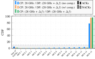
(a) $\Delta f=100$ MHz.

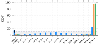
(b) $\Delta f=500$ MHz.

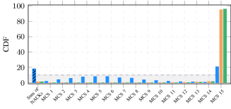
(c) $\Delta f=1$ GHz.

Figure 14: Histogram of UEs’ MCS usage in DL for different values of $\Delta f$ considering a gNB with a ULA with 256 antenna elements.

VI Conclusions

This paper proposed an efficient compensation method for beam squinting in repeater-assisted networks. From a link level point-of-view, we have shown that our proposed method is able to compensate for the beam squinting effect on the array gain in both azimuth and zenith for different values of frequency displacement and different antenna array configurations. As a consequence, from a system level point-of-view, we have shown through simulations that our proposal enables the NCR subband signaling operation. With our proposal, when transmitting data at a frequency different from the one in which the measurements are performed, we are able to keep UEs’ throughput at the same level as when the data transmission and channel measurement are performed at the same frequency. Furthermore, we have shown that, without a compensation, the perceived SINR, and so UEs’ throughput, can decrease substantially. For instance, considering an ULA with 256 antenna elements, $f_{c}=28\text{GHz}$ and $\Delta f=1\text{GHz}$. Without compensation, the SINR of the 10-percentile decreases by $20\text{\,}\mathrm{d}\mathrm{B}$ compared to the case when CP and DP operate at the same frequency. This is mainly due to the beam misalignment to the intended receiver as well as the increase in the interference to other receivers due to beam squinting. Such a degradation is fully compensated with our proposed method.

References

- [1] Mohamed Shehata et al. “Optical and Terahertz Wireless Technologies: the Race to 6G Communications” In IEEE Wireless Commun. 30.5, 2023, pp. 10–18 DOI: 10.1109/MWC.001.2300138
- [2] Nandana Rajatheva et al. “Scoring the Terabit/s Goal:Broadband Connectivity in 6G”, 2021 arXiv:2008.07220 [eess.SP]
- [3] Hao Guo et al. “A Comparison between Network-Controlled Repeaters and Reconfigurable Intelligent Surfaces”, 2022 arXiv:2211.06974 [cs.NI]
- [4] Gabriel Carlini Monte Silva et al. “System Level Evaluation of Network-Controlled Repeaters: Performance Improvement of Serving Cell and Interference Impact on Neighbor Cells”, 2023 arXiv:2306.11813 [eess.SY]
- [5] Victor Farias Monteiro et al. “Paving the Way Towards Mobile IAB: Problems, Solutions and Challenges” In IEEE Open J. Commu. Soc. 3, 2022, pp. 2347–2379 DOI: 10.1109/OJCOMS.2022.3224576
- [6] Charitha Madapatha et al. “On Integrated Access and Backhaul Networks: Current Status and Potentials” In IEEE Open J. Commu. Soc. 1, 2020, pp. 1374–1389 DOI: 10.1109/OJCOMS.2020.3022529
- [7] Zhen Chen et al. “Reconfigurable-Intelligent-Surface-Assisted B5G/6G Wireless Communications: Challenges, Solution, and Future Opportunities” In IEEE Communications Magazine 61.1, 2023, pp. 16–22 DOI: 10.1109/MCOM.002.2200047
- [8] 3GPP “Study on NR network-controlled repeaters” v.18.0.0, 2022 URL: http://www.3gpp.org/DynaReport/38867.htm
- [9] Xingqin Lin “An Overview of 5G Advanced Evolution in 3GPP Release 18” In IEEE Commun. Stand. Mag. 6.3, 2022, pp. 77–83 DOI: 10.1109/MCOMSTD.0001.2200001
- [10] 3GPP “3GPP Contribution R1-2207680: Control information for enabling NCR”, 2022 URL: https://www.3gpp.org/ftp/tsg_ran/WG1_RL1/TSGR1_110/Docs/R1-2207680.zip
- [11] Mingming Cai et al. “Effect of Wideband Beam Squint on Codebook Design in Phased-Array Wireless Systems” In Proc. of the IEEE Global Telecommun. Conf. (GLOBECOM), 2016, pp. 1–6 DOI: 10.1109/GLOCOM.2016.7841766
- [12] Feifei Gao et al. “Wideband Beamforming for Hybrid Massive MIMO Terahertz Communications” In IEEE J. Sel. Areas Commun. 39.6, 2021, pp. 1725–1740 DOI: 10.1109/JSAC.2021.3071822
- [13] Jingbo Tan and Linglong Dai “Delay-Phase Precoding for THz Massive MIMO with Beam Split” In Proc. of the IEEE Global Telecommun. Conf. (GLOBECOM), 2019, pp. 1–6 DOI: 10.1109/GLOBECOM38437.2019.9014304
- [14] Linglong Dai, Jingbo Tan, Zhi Chen and H. Poor “Delay-Phase Precoding for Wideband THz Massive MIMO” In IEEE Trans. Wireless Commun. 21.9, 2022, pp. 7271–7286 DOI: 10.1109/TWC.2022.3157315
- [15] Qian Wan, Jun Fang, Zhi Chen and Hongbin Li “Hybrid Precoding and Combining for Millimeter Wave/Sub-THz MIMO-OFDM Systems With Beam Squint Effects” In IEEE Trans. Veh. Commun. 70.8, 2021, pp. 8314–8319 DOI: 10.1109/TVT.2021.3093095
- [16] Bangzhao Zhai, Yilun Zhu, Aimin Tang and Xudong Wang “THzPrism: Frequency-Based Beam Spreading for Terahertz Communication Systems” In IEEE Wireless Commun. Lett. 9.6, 2020, pp. 897–900 DOI: 10.1109/LWC.2020.2974468
- [17] Wanming Hao et al. “The Far-/Near-Field Beam Squint and Solutions for THz Intelligent Reflecting Surface Communications” In IEEE Trans. Veh. Commun. 72.8, 2023, pp. 10107–10118 DOI: 10.1109/TVT.2023.3254153
- [18] Siqi Ma, Wenqian Shen, Jianping An and Lajos Hanzo “Wideband Channel Estimation for IRS-Aided Systems in the Face of Beam Squint” In IEEE Trans. Wireless Commun. 20.10, 2021, pp. 6240–6253 DOI: 10.1109/TWC.2021.3072694
- [19] Harry L. Trees “Optimum array processing” Wiley & Sons, 2002
- [20] Seyed Kasra Garakoui, Eric A.. Klumperink, Bram Nauta and Frank E. Vliet “Phased-array antenna beam squinting related to frequency dependency of delay circuits” In Proc. of the European Microwave Conf., 2011, pp. 1–9 DOI: 10.23919/EuMC.2011.6101846
- [21] Patrick Agyapong “Simulation guidelines”, 2013 URL: https://metis2020.com/wp-content/uploads/deliverables/METIS_D6.1_v1.pdf
- [22] 3GPP “Study on Channel Model for Frequencies from 0.5 to 100 GHz” v.17.1.0, 2022 URL: http://www.3gpp.org/DynaReport/38901.htm
- [23] Alexandre Matos Pessoa et al. “A Stochastic Channel Model With Dual Mobility for 5G Massive Networks” In IEEE Access 7, 2019, pp. 149971–149987 DOI: 10.1109/ACCESS.2019.2947407
- [24] Victor Farias Monteiro, Icaro Leonardo Silva and Francisco Rodrigo Porto Cavalcanti “5G Measurement Adaptation Based on Channel Hardening Occurrence” In IEEE Commun. Lett. 23.9, 2019, pp. 1598–1602 DOI: 10.1109/LCOMM.2019.2926268
- [25] 3GPP “NR; Physical layer measurements”, 2018 URL: http://www.3gpp.org/ftp/Specs/html-info/38215.htm
- [26] 3GPP “NR; Physical layer procedures for data” v.15.0.0, 2017 URL: http://www.3gpp.org/ftp/Specs/html-info/38214.htm