Quantum Simulation of SU(3) Lattice Yang Mills Theory at Leading Order in Large N
Abstract
A Hamiltonian lattice formulation of SU(3) gauge theory opens the possibility for quantum simulations of the non-perturbative dynamics of QCD. By parametrizing the gauge invariant Hilbert space in terms of plaquette degrees of freedom, we show how the Hilbert space and interactions can be expanded in inverse powers of . At leading order in this expansion, the Hamiltonian simplifies dramatically, both in the required size of the Hilbert space as well as the type of interactions involved. Adding a truncation of the resulting Hilbert space in terms of local energy states we give explicit constructions that allow simple representations of SU(3) gauge fields on qubits and qutrits. The limitations of these truncations are explored using Monte Carlo methods. This formulation allows a simulation of the real time dynamics of a SU(3) lattice gauge theory on a and lattice on ibm_torino with a CNOT depth of 113.
The real time dynamics of strongly coupled quantum field theories such as quantum chromodynamics (QCD) are relevant to many processes in high energy physics. These include phenomena such as hadronization, jet fragmentation, and the behavior of matter under extreme conditions such as in the early universe. The numerical study of QCD on a lattice using Monte-Carlo (MC) integration has enabled precision non-perturbative calculations of a number of observables [1, 2, 3, 4, 5, 6]. However, for many observables, Monte-Carlo integration is limited due to a sign problem. Hamiltonian lattice QCD formulations promise to circumvent these limitations, but are exponentially difficult to simulate on classical computers. Research in Hamiltonian formulations has gained in importance recently due to advances in the development of quantum computers based on a number of different platforms, such as superconducting qubits, trapped ions, and neutral atoms [7, 8, 9, 10, 11, 12, 13, 14, 15, 16, 17]. It is anticipated that simulations performed on quantum computers will be able to directly probe real-time dynamics with polynomially scaling computational costs [18, 19, 20, 21, 22, 23]. The continuous gauge fields need to be digitized to map them onto a quantum computer’s discrete degrees of freedom. Common basis choices for the Hilbert space of a LGT correspond to choosing on each link group elements (magnetic basis) [24, 25, 26, 27, 28, 29, 30, 31], group representations (electric basis) [32, 33, 34, 35, 36, 37, 38, 39, 40, 41, 42, 43, 44, 45, 46, 47, 48, 49, 50, 51, 52, 53, 54, 55, 55, 56, 57, 58, 59, 60, 61], or a mixture of the two [62, 63, 64, 65], and digitizations can be obtained in each of the choices. These formal developments have been used to perform a number of quantum simulations on existing hardware including simulations of the Schwinger model, QCD, SU(2) and SU(3) gauge theories on small lattices and some discrete groups [66, 45, 50, 48, 46, 44, 28, 67, 29, 49, 68, 69, 70, 71, 72, 73, 74, 75, 76, 77, 78, 79, 47, 80]. However, most quantum simulations of lattice gauge theories have been restricted to either small systems or one dimensional systems. Going beyond (1+1)D systems is limited by the complexity of implementing plaquette operators which are not present in one spatial dimension.
In this work we will use an electric basis, in which states are labeled by the representation of the gauge group at each link and gauge invariance can be implemented using local constraints that implement Gauss’s law at each lattice site. The electric basis can be digitized by truncating the allowed representations at each link, which amounts to limiting the local energy allowed. This can be done in a way that respects gauge invariance, and gauge invariance can be used to integrate out some unphysical states at the cost of a slight increase in the non-locality of the Hamiltonian [46].
In this work we add an expansion in the number of colors to the electric basis formulation. It is known that such a expansion leads to simplifications in perturbative QCD (for a review, see [81, 82]), and is a crucial ingredient in many calculational frameworks of QCD, most notably the parton shower approximation [83, 84]. While the physical value of is not particularly large, such expansions have been shown to be very successful phenomenologically [85, 83, 84, 86, 87]. Additionally, the large limit of QCD has been shown to be connected to models of quantum gravity through the AdS/CFT correspondence [88].
The large limit can be understood as a classical limit [89, 90] and by expanding in more non-classical features of the theory will be included in the quantum simulation. Note that the classical limit has a degree of freedom for each possible loop on the lattice which limits its applicability to simulating dynamics on classical computers [90, 91, 92].
The Kogut Susskind Hamiltonian describing pure SU(3) LGT is given by
| (1) |
where is the strong coupling constant, with the SU(3) chromo-electric field on link and is the trace over color indices of the product of parallel transporters on plaquette [93, 94, 95, 96]. In the electric basis, the Hilbert space on each link is spanned by states where is an irreducible representation of SU(3) and and label states in the representation acting from the left and right.
The SU(3) representation at each link on a point-split lattice can be labeled by the two quantum numbers and , due to SU(3) being a rank two group. A gauge invariant representation requires representations at each vertex to combine into a singlet. This is most easily accomplished using point-split vertices and requiring that the quantum numbers at each 3-point vertex add to zero. This has previously been used in formulations of q-deformed lattice gauge theories [97, 98] and is very similar to the approach taken in Loop String Hadron formulations [39, 40, 99, 41].
As explained in the supplemental material, an alternative labeling of a gauge invariant Hilbert state is obtained by specifying oriented closed loops, denoted by , and the way the arrows at each link having more than one loop pass through are combined, denoted by . A basis state can therefore be written as .
As explained in more detail in the supplemental material, the only physically relevant states have nonzero overlap with those obtained by acting on the electric vacuum state with an operator containing () powers of the plaquette operator () at each plaquette . While other gauge invariant states do exist, they are in different topological sectors and do not need to be represented on the quantum computer as different topological sectors do not interact. This operator allows us to define the state
| (2) |
The overlap can be expanded in powers of using the relation [100]
| (3) |
One finds at leading order in large
| (4) |
were counts the total number of plaquettes encircled by each loop . Therefore, the only overlap that survives in the large limit is the one with states for which each loop encircles exactly one plaquette, such that all . This leads to the final result that in the large limit each state can be specified by the number of single-plaquette loops in the positive and negative direction at each plaquette and at each link traversed by multiple of these loops.. These states are orthonormal to each other, such that the Hilbert space is spanned by the basis
| (5) |
Due to the suppression of larger loops, the dimension of the Hilbert space in the large limit is dramatically reduced. Another important simplification is that in this formulation no virtual point-splitting is required. Before we move on, we present the dimension and Casimir of a a representation . They are given by
| (6) |
So far, our discussion has not used any truncation of the Hilbert space. As already discussed, a standard way of truncating the Hilbert space is to limit the energy stored in each link of the lattice, which in turn limits the Hilbert space to those states for which the Casimir at each link is below a certain value. This truncation preserves all symmetries of the Hamiltonian, most importantly gauge invariance, which guarantees the truncated theory either to have a lattice spacing that freezes out or goes to theory with the correct gauge symmetry and matter content in the continuum limit [101]. Simulations of truncated theories have demonstrated the freezing out of the lattice spacing [102, 103, 104, 105, 106, 107], although some infrared properties of the theory can still be recovered [108]. At large , this truncation amounts to limiting the total value of at each link. The simplest non-trivial truncation is to require
| (7) |
which includes all links with Casimir . Given the large construction of the Hilbert space, this allows at most one loop excitation at each plaquette. Furthermore, a plaquette can only be excited if all adjacent plaquettes are in the ground state. The only allowed values for are then , or , and no specification of is necessary.
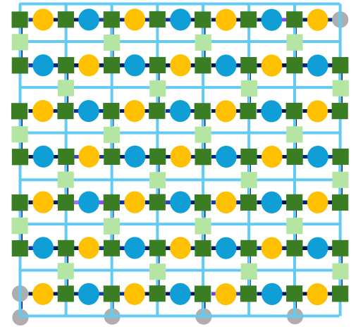
The Hilbert space at this truncation can therefore be described by assigning a qutrit to each plaquette in the lattice. The states of the qutrit will be labelled by , , and . Physical states are subject to the constraint that neighboring plaquettes are not simultaneously excited. For example, in a two plaquette system, the states and are physical while and are not, since it would give rise to the common link having . Similar constructions have been used to study SU(2) lattice gauge theory in the electric basis on plaquette chains and a hexagonal lattice [48, 109, 110, 111, 112, 113, 114]. However, note that the basis given here can work in higher spatial dimensions and with periodic boundary conditions as there is no potential double counting of states at this truncation unlike previous work on the hexagonal lattice.
If one truncates at leading order in and uses , the electric field operator for a link lying on plaquettes and at this truncation can be written as
| (8) |
where we have used the full expression of the Casimir of the fundamental representation . The plaquette operator at position is given by
| (9) |
where and () denotes the plaquette one position away in the () direction. These operators can be used to write down the Hamiltonian in Eq. (1) at this truncation.
This Hamiltonian has a CP symmetry that causes states with the anti-symmetric combination anywhere on the lattice to decouple from the rest of the Hilbert space. One can therefore perform separate simulations for the CP even and odd sector. By assigning , the CP (anti)symmetric subspace can be described by assigning a qubit to each plaquette instead of a qutrit. As already mentioned, physical states have the constraint that neighboring qubits cannot both be in the state. With this encoding, the Hamiltonian is given by
| (10) |
where and is the Pauli X operator acting on the qubit at plaquette . It is interesting to note that the plaquette operator at this truncation is a term. models have previously been studied as an effective Hamiltonian describing the low energy subspace of Rydberg atom arrays which can be described by Ising models [115, 116, 117]. It has been studied in the context of thermalization where the presence of scar states has been demonstrated [118, 119, 120, 121, 122]. Eq. (10) can be described as a limit of an Ising model with fields in the and directions and that in this regime the Ising model has been shown to demonstrate confinement [123, 124, 125]. This suggests that it may be possible to connect the presence of confinement in the Ising model to the physics of large Yang Mills.
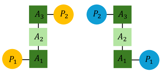
There are three representations with , namely , and , and a next truncation in the large limit should include all three of those states. However, taking into account subleading corrections, the representation with the second smallest Casimir at large is the anti-symmetric combination of two fundamental representations with . Note that in , this is just the representation. Changing the truncation to include this representation allows neighboring plaquettes to be excited and includes states with vertices that have three incoming or outgoing representations. As shown in more detail in the supplemental material, this truncation still fixes the representation on each link by the number of loops on the neighboring plaquettes, and each plaquette can still only be in the three possible states , and . A pair of neighboring plaquettes can only be in one of the following states , , , , , or . The Hilbert space is therefore still spanned by a qutrit at each plaquette.
At this truncation, the electric field operator on a link shared between plaquettes and is given by
| (11) |
The plaquette operator is given by
| (12) |
Using results in the supplemental material, it can be seen that for all and , and when the controls are not all , for transitions between allowed physical states where is the number of excited neighboring plaquettes.
The Hamiltonians obtained at the two truncations discussed above are both stoquastic [126]. This means that their static properties can be studied using Monte Carlo techniques without a sign problem. This allows us to study the effects of the truncations. MC calculations of the electric energy on a lattice with periodic boundary conditions at inverse temperature were performed. Details of the implementation are in the supplemental material.
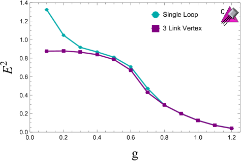
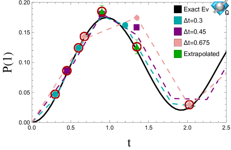
Fig. 1 shows the expectation of as a function of for the truncated Hamiltonians studied in this work 111The icons in the corners of plots indicate if classical or quantum compute resources were used to perform the calculation [153] and are available at https://iqus.uw.edu/resources/icons/ . As this figure shows, the truncated Hamiltonians are in agreement at large and discrepancies grow as is lowered. In addition to studying the effects of truncations, MC calculations can be used to generate ensembles of states that when averaged produce a thermal distribution [128, 129, 130, 131, 132]. These states can be initialized on quantum computers which would allow for studying dynamics of this theory at finite temperature without a sign problem. Additionally, many of the variables used in scale setting in traditional lattice QCD are defined in terms of Euclidean correlation functions which are difficult to access on quantum computers [133, 51, 134]. For these truncated Hamiltonians, classical MC calculations can be used to compute these variables to set the scale for a simulation with the same Hamiltonian on a quantum computer.
The size of the Hilbert space of this theory grows exponentially with the volume of thhe lattice and to study the dynamics at scale will ultimately require quantum computers. As an example of how the formalism introduced in this work can be used for quantum simulation, the Hamiltonian in Eq. (10) was simulated on IBM’s 133 qubit superconducting quantum computer ibm_torino [135, 136]. Due to the connectivity of the hardware, open boundary conditions were used. Time evolution was implemented using Trotterized time evolution operators. Errors in the calculation were suppressed using dynamical decoupling sequences and Pauli twirling [137, 138, 50, 48]. Errors in the gates were mitigated using operator decoherence renormalization and CNOT noise extrapolations [138, 50, 48, 77, 139, 140, 141, 142, 143]. Readout errors were mitigated using twirled readout error extinction (T-REX) [144]. Since the number of Trotter steps that can be run on quantum hardware is limited, we utilize multiple time step sizes to obtain results at more values. Increasing will increase the size of time discretization errors in the simulation, but this can be mitigated by choosing such that late time slices are sampled by multiple values of , which then allows an extrapolation to small . The details of the implementation of these techniques is described in the supplemental material.
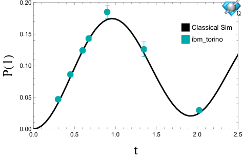
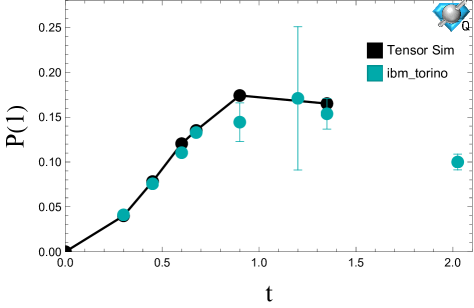
A lattice with was simulated using a set of 39 qubits on ibm_torino. Due to open boundary conditions, this lattice has plaquettes. 16 of the qubits were used to represent the Hilbert space of the theory and the remaining qubits are used to enable efficient communication between them. The system was initialized in the electric vacuum and the probability of a qubit being excited averaged over the lattice is shown in Fig. 2, showing results both from classical simulations of this relatively small system and from runs on quantum hardware using ibm_torino. We observe good agreement between the classical simulation and the results from ibm_torino. Note that this observable is proportional to the electric energy in the system, and previous work has used the evolution of the electric energy as a probe of thermalization times in SU(2) lattice gauge theory [145].
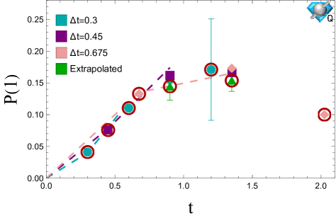
Having validated the quantum circuits for the lattice, an lattice with open boundary conditions was simulated on ibm_torino. This requires 49 qubits to represent the state of the system and the remaining qubits are used to enable communication between them. The average probability of a plaquette being excited is shown in Fig. 3. Simulating the time evolution for a system of this size is beyond the reach of brute force state vector simulation. Vacuum properties of large one dimensional systems can be simulated efficiently using tensor networks [146, 147, 148, 149, 150], however performing real time evolution requires resources that grow with evolution time. Scaling tensor network calculations to multiple spatial dimensions is practically challenging [151]. The black points in Fig. 3 show tensor network simulations of up to two Trotter steps of the circuits that were implemented on imb_torino using cuQuantum [152] on a single NVIDIA A100 GPU. Two Trotter steps took roughly one minute to run, however 3 Trotter steps did not finish running within 20 hours. For this reason, there is no extrapolation to in the classical simulation or classical data for 3 Trotter steps. Due to the lack of the extrapolation in the classical simulation and validation of the quantum circuits on a smaller lattice, it is expected that data from ibm_torino is a more accurate simulation of the dynamics of the system than the tensor network calculations. Note that further optimization of the classical simulation is likely to reduce the runtime, however this system is still in the regime where classical simulation is expected to be difficult. For reference, running and processing all of the quantum circuits for a single time step took roughly 7 minutes.
In this work, a large expansion was combined with electric basis truncations of the Kogut-Susskind Hamiltonian. This led to significant simplifications of the Hamiltonian and enabled a quantum simulation of SU(3) lattice gauge theory in multiple spatial dimensions. It is expected that this formalism can be extended to spatial dimensions and to include matter. Going to subleading order in and to larger truncations should also be possible systematically. The simplifications from truncating at some order in and success of large expansions may allow for near term simulations of phenomenologically relevant phenomena such as inelastic scattering, jet fragmentation or thermalization. Additionally, the connection of the large limit of gauge theories to quantum gravity may allow quantum simulations of these truncations to give insights into some models of quantum gravity.
Acknowledgements.
We would like to acknowledge helpful conversations with Ivan Burbano, Jesse Stryker, and Michael Kreshchuk. We would like to thank Martin Savage, Marc Illa, and Roland Farrell for many converstations related to quantum simulation. We would like to thank Aneesh Manohar for helpful discussions about large expansions. We would also like to acknowledge helpful conversations with Jad Halimeh about the emergence of models from certain limits of gauge theories. This material is based upon work supported by the U.S. Department of Energy, Office of Science, National Quantum Information Science Research Centers, Quantum Systems Accelerator. Additional support is acknowledged from the U.S. Department of Energy (DOE), Office of Science under contract DE-AC02-05CH11231, partially through Quantum Information Science Enabled Discovery (QuantISED) for High Energy Physics (KA2401032). This research used resources of the Oak Ridge Leadership Computing Facility (OLCF), which is a DOE Office of Science User Facility supported under Contract DE-AC05-00OR22725. We acknowledge the use of IBM Quantum services for this work. The views expressed are those of the authors, and do not reflect the official policy or position of IBM or the IBM Quantum team. This research used resources of the National Energy Research Scientific Computing Center, which is supported by the Office of Science of the U.S. Department of Energy under Contract No. DE-AC02-05CH11231.References
- Wilson [1974] K. G. Wilson, Confinement of quarks, Phys. Rev. D 10, 2445 (1974).
- Borsanyi et al. [2015] S. Borsanyi, S. Durr, Z. Fodor, C. Hoelbling, S. D. Katz, S. Krieg, L. Lellouch, T. Lippert, A. Portelli, K. K. Szabo, and B. C. Toth, Ab initio calculation of the neutron-proton mass difference, Science 347, 1452 (2015), https://www.science.org/doi/pdf/10.1126/science.1257050 .
- Karsch et al. [2003] F. Karsch, K. Redlich, and A. Tawfik, Hadron resonance mass spectrum and lattice QCD thermodynamics, The European Physical Journal C 29, 549 (2003).
- Tiburzi et al. [2017] B. C. Tiburzi, M. L. Wagman, F. Winter, E. Chang, Z. Davoudi, W. Detmold, K. Orginos, M. J. Savage, and P. E. Shanahan (NPLQCD Collaboration), Double- decay matrix elements from lattice quantum chromodynamics, Phys. Rev. D 96, 054505 (2017).
- Beane et al. [2015] S. R. Beane, E. Chang, W. Detmold, K. Orginos, A. Parreño, M. J. Savage, and B. C. Tiburzi (NPLQCD Collaboration), Ab initio calculation of the radiative capture process, Phys. Rev. Lett. 115, 132001 (2015).
- Savage et al. [2017] M. J. Savage, P. E. Shanahan, B. C. Tiburzi, M. L. Wagman, F. Winter, S. R. Beane, E. Chang, Z. Davoudi, W. Detmold, and K. Orginos (NPLQCD Collaboration), Proton-proton fusion and tritium decay from lattice quantum chromodynamics, Phys. Rev. Lett. 119, 062002 (2017).
- Huang et al. [2020] H.-L. Huang, D. Wu, D. Fan, and X. Zhu, Superconducting quantum computing: a review, Science China Information Sciences 63, 10.1007/s11432-020-2881-9 (2020).
- Bianchetti et al. [2010] R. Bianchetti, S. Filipp, M. Baur, J. M. Fink, C. Lang, L. Steffen, M. Boissonneault, A. Blais, and A. Wallraff, Control and tomography of a three level superconducting artificial atom, Phys. Rev. Lett. 105, 223601 (2010).
- Wang et al. [2022] C. Wang, I. Gonin, A. Grassellino, S. Kazakov, A. Romanenko, V. P. Yakovlev, and S. Zorzetti, High-efficiency microwave-optical quantum transduction based on a cavity electro-optic superconducting system with long coherence time, npj Quantum Information 8, 149 (2022).
- Wallraff et al. [2004] A. Wallraff, D. I. Schuster, A. Blais, L. Frunzio, R.-S. Huang, J. Majer, S. Kumar, S. M. Girvin, and R. J. Schoelkopf, Strong coupling of a single photon to a superconducting qubit using circuit quantum electrodynamics, Nature 431, 162 (2004).
- Chiorescu et al. [2004] I. Chiorescu, P. Bertet, K. Semba, Y. Nakamura, C. J. P. M. Harmans, and J. E. Mooij, Coherent dynamics of a flux qubit coupled to a harmonic oscillator, Nature 431, 159 (2004).
- Bruzewicz et al. [2019] C. D. Bruzewicz, J. Chiaverini, R. McConnell, and J. M. Sage, Trapped-ion quantum computing: Progress and challenges, Applied Physics Reviews 6, 021314 (2019).
- Henriet et al. [2020] L. Henriet, L. Beguin, A. Signoles, T. Lahaye, A. Browaeys, G.-O. Reymond, and C. Jurczak, Quantum computing with neutral atoms, Quantum 4, 327 (2020).
- Browaeys and Lahaye [2020] A. Browaeys and T. Lahaye, Many-body physics with individually controlled rydberg atoms, Nature Physics 16, 132 (2020).
- Barredo et al. [2020] D. Barredo, V. Lienhard, P. Scholl, S. de Lé séleuc, T. Boulier, A. Browaeys, and T. Lahaye, Three-dimensional trapping of individual rydberg atoms in ponderomotive bottle beam traps, Physical Review Letters 124, 10.1103/physrevlett.124.023201 (2020).
- Bluvstein et al. [2022] D. Bluvstein, H. Levine, G. Semeghini, T. T. Wang, S. Ebadi, M. Kalinowski, A. Keesling, N. Maskara, H. Pichler, M. Greiner, V. Vuletić, and M. D. Lukin, A quantum processor based on coherent transport of entangled atom arrays, Nature 604, 451 (2022).
- Bluvstein et al. [2023] D. Bluvstein, S. J. Evered, A. A. Geim, S. H. Li, H. Zhou, T. Manovitz, S. Ebadi, M. Cain, M. Kalinowski, D. Hangleiter, et al., Logical quantum processor based on reconfigurable atom arrays, Nature , 1 (2023).
- Feynman [1981] R. P. Feynman, Simulating physics with computers, 1981, International Journal of Theoretical Physics 21 (1981).
- Bauer et al. [2023a] C. W. Bauer, Z. Davoudi, A. B. Balantekin, T. Bhattacharya, M. Carena, W. A. de Jong, P. Draper, A. El-Khadra, N. Gemelke, M. Hanada, D. Kharzeev, H. Lamm, Y.-Y. Li, J. Liu, M. Lukin, Y. Meurice, C. Monroe, B. Nachman, G. Pagano, J. Preskill, E. Rinaldi, A. Roggero, D. I. Santiago, M. J. Savage, I. Siddiqi, G. Siopsis, D. Van Zanten, N. Wiebe, Y. Yamauchi, K. Yeter-Aydeniz, and S. Zorzetti, Quantum simulation for high-energy physics, PRX Quantum 4, 10.1103/prxquantum.4.027001 (2023a).
- Humble et al. [2022a] T. S. Humble, A. Delgado, R. Pooser, C. Seck, R. Bennink, V. Leyton-Ortega, C. C. J. Wang, E. Dumitrescu, T. Morris, K. Hamilton, D. Lyakh, P. Date, Y. Wang, N. A. Peters, K. J. Evans, M. Demarteau, A. McCaskey, T. Nguyen, S. Clark, M. Reville, A. D. Meglio, M. Grossi, S. Vallecorsa, K. Borras, K. Jansen, and D. Krücker, Snowmass white paper: Quantum computing systems and software for high-energy physics research (2022a), arXiv:2203.07091 [quant-ph] .
- Humble et al. [2022b] T. S. Humble, G. N. Perdue, and M. J. Savage, Snowmass computational frontier: Topical group report on quantum computing (2022b), arXiv:2209.06786 [quant-ph] .
- Beck et al. [2023] D. Beck, J. Carlson, Z. Davoudi, J. Formaggio, S. Quaglioni, M. Savage, J. Barata, T. Bhattacharya, M. Bishof, I. Cloet, A. Delgado, M. DeMarco, C. Fink, A. Florio, M. Francois, D. Grabowska, S. Hoogerheide, M. Huang, K. Ikeda, M. Illa, K. Joo, D. Kharzeev, K. Kowalski, W. K. Lai, K. Leach, B. Loer, I. Low, J. Martin, D. Moore, T. Mehen, N. Mueller, J. Mulligan, P. Mumm, F. Pederiva, R. Pisarski, M. Ploskon, S. Reddy, G. Rupak, H. Singh, M. Singh, I. Stetcu, J. Stryker, P. Szypryt, S. Valgushev, B. VanDevender, S. Watkins, C. Wilson, X. Yao, A. Afanasev, A. B. Balantekin, A. Baroni, R. Bunker, B. Chakraborty, I. Chernyshev, V. Cirigliano, B. Clark, S. K. Dhiman, W. Du, D. Dutta, R. Edwards, A. Flores, A. Galindo-Uribarri, R. F. G. Ruiz, V. Gueorguiev, F. Guo, E. Hansen, H. Hernandez, K. Hattori, P. Hauke, M. Hjorth-Jensen, K. Jankowski, C. Johnson, D. Lacroix, D. Lee, H.-W. Lin, X. Liu, F. J. Llanes-Estrada, J. Looney, M. Lukin, A. Mercenne, J. Miller, E. Mottola, B. Mueller, B. Nachman, J. Negele, J. Orrell, A. Patwardhan, D. Phillips, S. Poole, I. Qualters, M. Rumore, T. Schaefer, J. Scott, R. Singh, J. Vary, J.-J. Galvez-Viruet, K. Wendt, H. Xing, L. Yang, G. Young, and F. Zhao, Quantum information science and technology for nuclear physics. input into u.s. long-range planning, 2023 (2023), arXiv:2303.00113 [nucl-ex] .
- Meglio et al. [2023] A. D. Meglio, K. Jansen, I. Tavernelli, C. Alexandrou, S. Arunachalam, C. W. Bauer, K. Borras, S. Carrazza, A. Crippa, V. Croft, R. de Putter, A. Delgado, V. Dunjko, D. J. Egger, E. Fernandez-Combarro, E. Fuchs, L. Funcke, D. Gonzalez-Cuadra, M. Grossi, J. C. Halimeh, Z. Holmes, S. Kuhn, D. Lacroix, R. Lewis, D. Lucchesi, M. L. Martinez, F. Meloni, A. Mezzacapo, S. Montangero, L. Nagano, V. Radescu, E. R. Ortega, A. Roggero, J. Schuhmacher, J. Seixas, P. Silvi, P. Spentzouris, F. Tacchino, K. Temme, K. Terashi, J. Tura, C. Tuysuz, S. Vallecorsa, U.-J. Wiese, S. Yoo, and J. Zhang, Quantum computing for high-energy physics: State of the art and challenges. summary of the qc4hep working group (2023), arXiv:2307.03236 [quant-ph] .
- Alexandru et al. [2019] A. Alexandru, P. F. Bedaque, S. Harmalkar, H. Lamm, S. Lawrence, and N. C. Warrington (NuQS Collaboration), Gluon field digitization for quantum computers, Phys. Rev. D 100, 114501 (2019).
- Lamm et al. [2019] H. Lamm, S. Lawrence, and Y. Yamauchi (NuQS Collaboration), General methods for digital quantum simulation of gauge theories, Phys. Rev. D 100, 034518 (2019).
- Ji et al. [2020] Y. Ji, H. Lamm, and S. Zhu (NuQS Collaboration), Gluon field digitization via group space decimation for quantum computers, Phys. Rev. D 102, 114513 (2020).
- Alexandru et al. [2022] A. Alexandru, P. F. Bedaque, R. Brett, and H. Lamm, Spectrum of digitized qcd: Glueballs in a gauge theory, Phys. Rev. D 105, 114508 (2022).
- Alam et al. [2022] M. S. Alam, S. Hadfield, H. Lamm, and A. C. Y. Li (SQMS Collaboration), Primitive quantum gates for dihedral gauge theories, Phys. Rev. D 105, 114501 (2022).
- Gustafson et al. [2022] E. J. Gustafson, H. Lamm, F. Lovelace, and D. Musk, Primitive quantum gates for an discrete subgroup: Binary tetrahedral, Phys. Rev. D 106, 114501 (2022).
- Zache et al. [2023a] T. V. Zache, D. González-Cuadra, and P. Zoller, Fermion-qudit quantum processors for simulating lattice gauge theories with matter, Quantum 7, 1140 (2023a).
- González-Cuadra et al. [2022] D. González-Cuadra, T. V. Zache, J. Carrasco, B. Kraus, and P. Zoller, Hardware efficient quantum simulation of non-abelian gauge theories with qudits on rydberg platforms, Phys. Rev. Lett. 129, 160501 (2022).
- Byrnes and Yamamoto [2006] T. Byrnes and Y. Yamamoto, Simulating lattice gauge theories on a quantum computer, Phys. Rev. A 73, 022328 (2006).
- Zohar et al. [2012] E. Zohar, J. I. Cirac, and B. Reznik, Simulating compact quantum electrodynamics with ultracold atoms: Probing confinement and nonperturbative effects, Phys. Rev. Lett. 109, 125302 (2012).
- Zohar et al. [2013a] E. Zohar, J. I. Cirac, and B. Reznik, Quantum simulations of gauge theories with ultracold atoms: Local gauge invariance from angular-momentum conservation, Phys. Rev. A 88, 023617 (2013a).
- Zohar et al. [2013b] E. Zohar, J. I. Cirac, and B. Reznik, Cold-atom quantum simulator for su(2) yang-mills lattice gauge theory, Phys. Rev. Lett. 110, 125304 (2013b).
- Zohar and Burrello [2015] E. Zohar and M. Burrello, Formulation of lattice gauge theories for quantum simulations, Phys. Rev. D 91, 054506 (2015).
- Zohar et al. [2015] E. Zohar, J. I. Cirac, and B. Reznik, Quantum simulations of lattice gauge theories using ultracold atoms in optical lattices, Reports on Progress in Physics 79, 014401 (2015).
- Zohar [2021] E. Zohar, Quantum simulation of lattice gauge theories in more than one space dimension—requirements, challenges and methods, Philosophical Transactions of the Royal Society A: Mathematical, Physical and Engineering Sciences 380, 10.1098/rsta.2021.0069 (2021).
- Raychowdhury and Stryker [2020a] I. Raychowdhury and J. R. Stryker, Solving gauss’s law on digital quantum computers with loop-string-hadron digitization, Phys. Rev. Res. 2, 033039 (2020a).
- Raychowdhury and Stryker [2020b] I. Raychowdhury and J. R. Stryker, Loop, string, and hadron dynamics in su(2) hamiltonian lattice gauge theories, Phys. Rev. D 101, 114502 (2020b).
- Kadam et al. [2023] S. V. Kadam, I. Raychowdhury, and J. R. Stryker, Loop-string-hadron formulation of an su(3) gauge theory with dynamical quarks, Phys. Rev. D 107, 094513 (2023).
- Shaw et al. [2020] A. F. Shaw, P. Lougovski, J. R. Stryker, and N. Wiebe, Quantum algorithms for simulating the lattice schwinger model, Quantum 4, 306 (2020).
- Ciavarella et al. [2022] A. Ciavarella, N. Klco, and M. J. Savage, Some conceptual aspects of operator design for quantum simulations of non-abelian lattice gauge theories (2022), arXiv:2203.11988 [quant-ph] .
- Ciavarella and Chernyshev [2022] A. N. Ciavarella and I. A. Chernyshev, Preparation of the su(3) lattice yang-mills vacuum with variational quantum methods, Phys. Rev. D 105, 074504 (2022).
- Klco et al. [2020] N. Klco, M. J. Savage, and J. R. Stryker, Su(2) non-abelian gauge field theory in one dimension on digital quantum computers, Phys. Rev. D 101, 074512 (2020).
- Ciavarella et al. [2021] A. Ciavarella, N. Klco, and M. J. Savage, Trailhead for quantum simulation of su(3) yang-mills lattice gauge theory in the local multiplet basis, Phys. Rev. D 103, 094501 (2021).
- Kavaki and Lewis [2024] A. H. Z. Kavaki and R. Lewis, From square plaquettes to triamond lattices for su(2) gauge theory (2024), arXiv:2401.14570 [hep-lat] .
- Rahman et al. [2022] S. A. Rahman, R. Lewis, E. Mendicelli, and S. Powell, Real time evolution and a traveling excitation in su(2) pure gauge theory on a quantum computer (2022), arXiv:2210.11606 [hep-lat] .
- Atas et al. [2021] Y. Y. Atas, J. Zhang, R. Lewis, A. Jahanpour, J. F. Haase, and C. A. Muschik, SU(2) hadrons on a quantum computer via a variational approach, Nature Communications 12, 10.1038/s41467-021-26825-4 (2021).
- A Rahman et al. [2022] S. A Rahman, R. Lewis, E. Mendicelli, and S. Powell, Self-mitigating trotter circuits for su(2) lattice gauge theory on a quantum computer, Phys. Rev. D 106, 074502 (2022).
- Paulson et al. [2021] D. Paulson, L. Dellantonio, J. F. Haase, A. Celi, A. Kan, A. Jena, C. Kokail, R. van Bijnen, K. Jansen, P. Zoller, and C. A. Muschik, Simulating 2d effects in lattice gauge theories on a quantum computer, PRX Quantum 2, 030334 (2021).
- Halimeh et al. [2023] J. C. Halimeh, L. Homeier, A. Bohrdt, and F. Grusdt, Spin exchange-enabled quantum simulator for large-scale non-abelian gauge theories (2023), arXiv:2305.06373 [cond-mat.quant-gas] .
- Meurice [2021] Y. Meurice, Theoretical methods to design and test quantum simulators for the compact abelian higgs model, Phys. Rev. D 104, 094513 (2021).
- Davoudi et al. [2020] Z. Davoudi, M. Hafezi, C. Monroe, G. Pagano, A. Seif, and A. Shaw, Towards analog quantum simulations of lattice gauge theories with trapped ions, Phys. Rev. Res. 2, 023015 (2020).
- Davoudi et al. [2021] Z. Davoudi, I. Raychowdhury, and A. Shaw, Search for efficient formulations for hamiltonian simulation of non-abelian lattice gauge theories, Phys. Rev. D 104, 074505 (2021).
- Belyansky et al. [2023] R. Belyansky, S. Whitsitt, N. Mueller, A. Fahimniya, E. R. Bennewitz, Z. Davoudi, and A. V. Gorshkov, High-energy collision of quarks and hadrons in the schwinger model: From tensor networks to circuit qed (2023), arXiv:2307.02522 [quant-ph] .
- Berenstein and Kawai [2023] D. Berenstein and H. Kawai, Integrable spin chains from large- qcd at strong coupling (2023), arXiv:2308.11716 [hep-th] .
- Rigobello et al. [2023] M. Rigobello, G. Magnifico, P. Silvi, and S. Montangero, Hadrons in (1+1)d hamiltonian hardcore lattice qcd (2023), arXiv:2308.04488 [hep-lat] .
- Kane et al. [2024] C. F. Kane, N. Gomes, and M. Kreshchuk, Nearly-optimal state preparation for quantum simulations of lattice gauge theories (2024), arXiv:2310.13757 [quant-ph] .
- Hariprakash et al. [2023] S. Hariprakash, N. S. Modi, M. Kreshchuk, C. F. Kane, and C. W. Bauer, Strategies for simulating time evolution of hamiltonian lattice field theories (2023), arXiv:2312.11637 [quant-ph] .
- Su et al. [2024] G.-X. Su, J. Osborne, and J. C. Halimeh, A cold-atom particle collider (2024), arXiv:2401.05489 [cond-mat.quant-gas] .
- Grabowska et al. [2023] D. M. Grabowska, C. Kane, B. Nachman, and C. W. Bauer, Overcoming exponential scaling with system size in trotter-suzuki implementations of constrained hamiltonians: 2+1 u(1) lattice gauge theories (2023), arXiv:2208.03333 [quant-ph] .
- Bauer and Grabowska [2023] C. W. Bauer and D. M. Grabowska, Efficient representation for simulating u(1) gauge theories on digital quantum computers at all values of the coupling, Phys. Rev. D 107, L031503 (2023).
- Kane et al. [2022] C. Kane, D. M. Grabowska, B. Nachman, and C. W. Bauer, Efficient quantum implementation of 2+1 u(1) lattice gauge theories with gauss law constraints (2022), arXiv:2211.10497 [quant-ph] .
- Bauer et al. [2023b] C. W. Bauer, I. D’Andrea, M. Freytsis, and D. M. Grabowska, A new basis for hamiltonian su(2) simulations (2023b), arXiv:2307.11829 [hep-ph] .
- Martinez et al. [2016] E. A. Martinez, C. A. Muschik, P. Schindler, D. Nigg, A. Erhard, M. Heyl, P. Hauke, M. Dalmonte, T. Monz, P. Zoller, and R. Blatt, Real-time dynamics of lattice gauge theories with a few-qubit quantum computer, Nature 534, 516 (2016).
- Illa and Savage [2022] M. Illa and M. J. Savage, Basic Elements for Simulations of Standard Model Physics with Quantum Annealers: Multigrid and Clock States, Phys. Rev. A 106, 052605 (2022), arXiv:2202.12340 [quant-ph] .
- Farrell et al. [2023a] R. C. Farrell, I. A. Chernyshev, S. J. M. Powell, N. A. Zemlevskiy, M. Illa, and M. J. Savage, Preparations for quantum simulations of quantum chromodynamics in dimensions. i. axial gauge, Phys. Rev. D 107, 054512 (2023a).
- Farrell et al. [2023b] R. C. Farrell, I. A. Chernyshev, S. J. M. Powell, N. A. Zemlevskiy, M. Illa, and M. J. Savage, Preparations for quantum simulations of quantum chromodynamics in dimensions. ii. single-baryon -decay in real time, Phys. Rev. D 107, 054513 (2023b).
- Atas et al. [2022] Y. Y. Atas, J. F. Haase, J. Zhang, V. Wei, S. M. L. Pfaendler, R. Lewis, and C. A. Muschik, Real-time evolution of SU(3) hadrons on a quantum computer (2022), arXiv:2207.03473 [quant-ph] .
- Yang et al. [2020] B. Yang, H. Sun, R. Ott, H.-Y. Wang, T. V. Zache, J. C. Halimeh, Z.-S. Yuan, P. Hauke, and J.-W. Pan, Observation of gauge invariance in a 71-site bose–hubbard quantum simulator, Nature 587, 392 (2020).
- Zhou et al. [2022] Z.-Y. Zhou, G.-X. Su, J. C. Halimeh, R. Ott, H. Sun, P. Hauke, B. Yang, Z.-S. Yuan, J. Berges, and J.-W. Pan, Thermalization dynamics of a gauge theory on a quantum simulator, Science 377, 311 (2022).
- Su et al. [2023] G.-X. Su, H. Sun, A. Hudomal, J.-Y. Desaules, Z.-Y. Zhou, B. Yang, J. C. Halimeh, Z.-S. Yuan, Z. Papić , and J.-W. Pan, Observation of many-body scarring in a bose-hubbard quantum simulator, Physical Review Research 5, 10.1103/physrevresearch.5.023010 (2023).
- Zhang et al. [2023] W.-Y. Zhang, Y. Liu, Y. Cheng, M.-G. He, H.-Y. Wang, T.-Y. Wang, Z.-H. Zhu, G.-X. Su, Z.-Y. Zhou, Y.-G. Zheng, H. Sun, B. Yang, P. Hauke, W. Zheng, J. C. Halimeh, Z.-S. Yuan, and J.-W. Pan, Observation of microscopic confinement dynamics by a tunable topological -angle (2023), arXiv:2306.11794 [cond-mat.quant-gas] .
- Mildenberger et al. [2022] J. Mildenberger, W. Mruczkiewicz, J. C. Halimeh, Z. Jiang, and P. Hauke, Probing confinement in a lattice gauge theory on a quantum computer (2022), arXiv:2203.08905 [quant-ph] .
- Ciavarella [2023] A. N. Ciavarella, Quantum simulation of lattice qcd with improved hamiltonians, Phys. Rev. D 108, 094513 (2023).
- Farrell et al. [2023c] R. C. Farrell, M. Illa, A. N. Ciavarella, and M. J. Savage, Scalable circuits for preparing ground states on digital quantum computers: The schwinger model vacuum on 100 qubits (2023c), arXiv:2308.04481 [quant-ph] .
- Farrell et al. [2024] R. C. Farrell, M. Illa, A. N. Ciavarella, and M. J. Savage, Quantum simulations of hadron dynamics in the schwinger model using 112 qubits (2024), arXiv:2401.08044 [quant-ph] .
- Charles et al. [2023] C. Charles, E. J. Gustafson, E. Hardt, F. Herren, N. Hogan, H. Lamm, S. Starecheski, R. S. V. de Water, and M. L. Wagman, Simulating lattice gauge theory on a quantum computer (2023), arXiv:2305.02361 [hep-lat] .
- Mueller et al. [2023] N. Mueller, J. A. Carolan, A. Connelly, Z. Davoudi, E. F. Dumitrescu, and K. Yeter-Aydeniz, Quantum computation of dynamical quantum phase transitions and entanglement tomography in a lattice gauge theory, PRX Quantum 4, 030323 (2023).
- Lucini and Panero [2013] B. Lucini and M. Panero, Su(n) gauge theories at large n, Physics Reports 526, 93 (2013), sU(N) gauge theories at large N.
- Manohar [1998] A. V. Manohar, Large N QCD, in Les Houches Summer School in Theoretical Physics, Session 68: Probing the Standard Model of Particle Interactions (1998) pp. 1091–1169, arXiv:hep-ph/9802419 .
- Sjostrand et al. [2006] T. Sjostrand, S. Mrenna, and P. Z. Skands, PYTHIA 6.4 Physics and Manual, JHEP 05, 026, arXiv:hep-ph/0603175 .
- Bahr et al. [2008] M. Bahr et al., Herwig++ Physics and Manual, Eur. Phys. J. C 58, 639 (2008), arXiv:0803.0883 [hep-ph] .
- ’t Hooft [1974] G. ’t Hooft, A Planar Diagram Theory for Strong Interactions, Nucl. Phys. B 72, 461 (1974).
- PICH [2002] A. PICH, Colourless mesons in a polychromatic world, in Phenomenology of Large Nc QCD (WORLD SCIENTIFIC, 2002).
- Kaplan and Savage [1996] D. B. Kaplan and M. J. Savage, The spin-flavor dependence of nuclear forces from large-n qcd, Physics Letters B 365, 244 (1996).
- Maldacena [1999] J. Maldacena, The large-n limit of superconformal field theories and supergravity, International journal of theoretical physics 38, 1113 (1999).
- Witten [1980] E. Witten, The 1/n expansion in atomic and particle physics, in Recent Developments in Gauge Theories, edited by G. Hooft, C. Itzykson, A. Jaffe, H. Lehmann, P. K. Mitter, I. M. Singer, and R. Stora (Springer US, Boston, MA, 1980) pp. 403–419.
- Yaffe [1982] L. G. Yaffe, Large limits as classical mechanics, Rev. Mod. Phys. 54, 407 (1982).
- Jevicki et al. [1983] A. Jevicki, O. Karim, J. Rodrigues, and H. Levine, Loop space hamiltonians and numerical methods for large-n gauge theories, Nuclear Physics B 213, 169 (1983).
- Jevicki et al. [1984] A. Jevicki, O. Karim, J. Rodrigues, and H. Levine, Loop-space hamiltonians and numerical methods for large-n gauge theories (ii), Nuclear Physics B 230, 299 (1984).
- Kogut and Susskind [1975] J. Kogut and L. Susskind, Hamiltonian formulation of wilson’s lattice gauge theories, Phys. Rev. D 11, 395 (1975).
- Kogut [1979] J. B. Kogut, An introduction to lattice gauge theory and spin systems, Rev. Mod. Phys. 51, 659 (1979).
- Banks et al. [1977] T. Banks, S. Raby, L. Susskind, J. Kogut, D. R. T. Jones, P. N. Scharbach, and D. K. Sinclair, Strong-coupling calculations of the hadron spectrum of quantum chromodynamics, Phys. Rev. D 15, 1111 (1977).
- Jones et al. [1979] D. Jones, R. Kenway, J. Kogut, and D. Sinclair, Lattice gauge theory calculations using an improved strong-coupling expansion and matrix padé approximants, Nuclear Physics B 158, 102 (1979).
- Zache et al. [2023b] T. V. Zache, D. González-Cuadra, and P. Zoller, Quantum and classical spin-network algorithms for -deformed kogut-susskind gauge theories, Phys. Rev. Lett. 131, 171902 (2023b).
- Hayata and Hidaka [2023] T. Hayata and Y. Hidaka, deformed formulation of hamiltonian su(3) yang-mills theory (2023), arXiv:2306.12324 [hep-lat] .
- Davoudi et al. [2023] Z. Davoudi, A. F. Shaw, and J. R. Stryker, General quantum algorithms for hamiltonian simulation with applications to a non-abelian lattice gauge theory, Quantum 7, 1213 (2023).
- Weingarten [2008] D. Weingarten, Asymptotic behavior of group integrals in the limit of infinite rank, Journal of Mathematical Physics 19, 999 (2008), https://pubs.aip.org/aip/jmp/article-pdf/19/5/999/11195862/999_1_online.pdf .
- Levin and Wen [2005] M. A. Levin and X.-G. Wen, String-net condensation: A physical mechanism for topological phases, Phys. Rev. B 71, 045110 (2005).
- Bañuls et al. [2017] M. C. Bañuls, K. Cichy, J. I. Cirac, K. Jansen, and S. Kühn, Efficient basis formulation for ()-dimensional su(2) lattice gauge theory: Spectral calculations with matrix product states, Phys. Rev. X 7, 041046 (2017).
- Haase et al. [2021] J. F. Haase, L. Dellantonio, A. Celi, D. Paulson, A. Kan, K. Jansen, and C. A. Muschik, A resource efficient approach for quantum and classical simulations of gauge theories in particle physics, Quantum 5, 393 (2021).
- Bruckmann et al. [2019] F. Bruckmann, K. Jansen, and S. Kühn, O(3) nonlinear sigma model in dimensions with matrix product states, Phys. Rev. D 99, 074501 (2019).
- Zache et al. [2022] T. V. Zache, M. Van Damme, J. C. Halimeh, P. Hauke, and D. Banerjee, Toward the continuum limit of a quantum link schwinger model, Phys. Rev. D 106, L091502 (2022).
- Alexandru et al. [2023] A. Alexandru, P. F. Bedaque, A. Carosso, M. J. Cervia, and A. Sheng, Qubitization strategies for bosonic field theories, Phys. Rev. D 107, 034503 (2023).
- Araz et al. [2023] J. Y. Araz, S. Schenk, and M. Spannowsky, Toward a quantum simulation of nonlinear sigma models with a topological term, Phys. Rev. A 107, 032619 (2023).
- Liu et al. [2023] H. Liu, T. Bhattacharya, S. Chandrasekharan, and R. Gupta, Phases of 2d massless qcd with qubit regularization (2023), arXiv:2312.17734 [hep-lat] .
- Müller and Yao [2023] B. Müller and X. Yao, Simple hamiltonian for quantum simulation of strongly coupled su(2) lattice gauge theory on a honeycomb lattice, Phys. Rev. D 108, 094505 (2023).
- Ebner et al. [2024a] L. Ebner, A. Schäfer, C. Seidl, B. Müller, and X. Yao, Eigenstate thermalization in ()-dimensional su(2) lattice gauge theory, Phys. Rev. D 109, 014504 (2024a).
- Yao [2023] X. Yao, Su(2) gauge theory in dimensions on a plaquette chain obeys the eigenstate thermalization hypothesis, Phys. Rev. D 108, L031504 (2023).
- Yao et al. [2023] X. Yao, L. Ebner, B. Müller, A. Schäfer, and C. Seidl, Testing eigenstate thermalization hypothesis for non-abelian gauge theories (2023), arXiv:2312.13408 [hep-lat] .
- Ebner et al. [2024b] L. Ebner, A. Schäfer, C. Seidl, B. Müller, and X. Yao, Entanglement entropy of ()-dimensional su(2) lattice gauge theory (2024b), arXiv:2401.15184 [hep-lat] .
- Turro et al. [2024] F. Turro, A. Ciavarella, and X. Yao, Classical and quantum computing of shear viscosity for su(2) gauge theory (2024), arXiv:2402.04221 [hep-lat] .
- Ebadi et al. [2021] S. Ebadi, T. T. Wang, H. Levine, A. Keesling, G. Semeghini, A. Omran, D. Bluvstein, R. Samajdar, H. Pichler, W. W. Ho, S. Choi, S. Sachdev, M. Greiner, V. Vuletić, and M. D. Lukin, Quantum phases of matter on a 256-atom programmable quantum simulator, Nature 595, 227 (2021).
- Semeghini et al. [2021] G. Semeghini, H. Levine, A. Keesling, S. Ebadi, T. T. Wang, D. Bluvstein, R. Verresen, H. Pichler, M. Kalinowski, R. Samajdar, A. Omran, S. Sachdev, A. Vishwanath, M. Greiner, V. Vuletić, and M. D. Lukin, Probing topological spin liquids on a programmable quantum simulator, Science 374, 1242 (2021), https://www.science.org/doi/pdf/10.1126/science.abi8794 .
- Omran et al. [2019] A. Omran, H. Levine, A. Keesling, G. Semeghini, T. T. Wang, S. Ebadi, H. Bernien, A. S. Zibrov, H. Pichler, S. Choi, J. Cui, M. Rossignolo, P. Rembold, S. Montangero, T. Calarco, M. Endres, M. Greiner, V. Vuletić , and M. D. Lukin, Generation and manipulation of schrödinger cat states in rydberg atom arrays, Science 365, 570 (2019).
- Nandkishore and Huse [2015] R. Nandkishore and D. A. Huse, Many-body localization and thermalization in quantum statistical mechanics, Annual Review of Condensed Matter Physics 6, 15 (2015), https://doi.org/10.1146/annurev-conmatphys-031214-014726 .
- Choi et al. [2019] S. Choi, C. J. Turner, H. Pichler, W. W. Ho, A. A. Michailidis, Z. Papić, M. Serbyn, M. D. Lukin, and D. A. Abanin, Emergent su(2) dynamics and perfect quantum many-body scars, Phys. Rev. Lett. 122, 220603 (2019).
- Moudgalya et al. [2022] S. Moudgalya, B. A. Bernevig, and N. Regnault, Quantum many-body scars and hilbert space fragmentation: a review of exact results, Reports on Progress in Physics 85, 086501 (2022).
- Chandran et al. [2023] A. Chandran, T. Iadecola, V. Khemani, and R. Moessner, Quantum many-body scars: A quasiparticle perspective, Annual Review of Condensed Matter Physics 14, 443 (2023), https://doi.org/10.1146/annurev-conmatphys-031620-101617 .
- Surace et al. [2020] F. M. Surace, P. P. Mazza, G. Giudici, A. Lerose, A. Gambassi, and M. Dalmonte, Lattice gauge theories and string dynamics in rydberg atom quantum simulators, Phys. Rev. X 10, 021041 (2020).
- Kormos et al. [2016] M. Kormos, M. Collura, G. Takács, and P. Calabrese, Real-time confinement following a quantum quench to a non-integrable model, Nature Physics 13, 246 (2016).
- James et al. [2019] A. J. A. James, R. M. Konik, and N. J. Robinson, Nonthermal states arising from confinement in one and two dimensions, Phys. Rev. Lett. 122, 130603 (2019).
- Robinson et al. [2019] N. J. Robinson, A. J. A. James, and R. M. Konik, Signatures of rare states and thermalization in a theory with confinement, Phys. Rev. B 99, 195108 (2019).
- Bravyi et al. [2007] S. Bravyi, D. P. DiVincenzo, R. I. Oliveira, and B. M. Terhal, The complexity of stoquastic local hamiltonian problems (2007), arXiv:quant-ph/0606140 [quant-ph] .
- Note [1] The icons in the corners of plots indicate if classical or quantum compute resources were used to perform the calculation [153] and are available at https://iqus.uw.edu/resources/icons/.
- Lamm and Lawrence [2018] H. Lamm and S. Lawrence, Simulation of nonequilibrium dynamics on a quantum computer, Phys. Rev. Lett. 121, 170501 (2018).
- Harmalkar et al. [2020] S. Harmalkar, H. Lamm, and S. Lawrence, Quantum simulation of field theories without state preparation (2020), arXiv:2001.11490 [hep-lat] .
- Gustafson and Lamm [2021] E. J. Gustafson and H. Lamm, Toward quantum simulations of gauge theory without state preparation, Phys. Rev. D 103, 054507 (2021).
- Blunt et al. [2014] N. S. Blunt, T. W. Rogers, J. S. Spencer, and W. M. C. Foulkes, Density-matrix quantum monte carlo method, Phys. Rev. B 89, 245124 (2014).
- Saroni et al. [2023] J. Saroni, H. Lamm, P. P. Orth, and T. Iadecola, Reconstructing thermal quantum quench dynamics from pure states, Phys. Rev. B 108, 134301 (2023).
- Sommer [2014] R. Sommer, Scale setting in lattice qcd (2014), arXiv:1401.3270 [hep-lat] .
- Ciavarella et al. [2023] A. N. Ciavarella, S. Caspar, H. Singh, and M. J. Savage, Preparation for quantum simulation of the -dimensional o(3) nonlinear model using cold atoms, Phys. Rev. A 107, 042404 (2023).
- Aleksandrowicz et al. [2019] G. Aleksandrowicz, T. Alexander, P. Barkoutsos, L. Bello, Y. Ben-Haim, D. Bucher, F. J. Cabrera-Hernández, J. Carballo-Franquis, A. Chen, C.-F. Chen, et al., Qiskit: An open-source framework for quantum computing, Accessed on: Mar 16 (2019).
- IBM Quantum Experience [2023] IBM Quantum Experience, ibm_torino v1.0.2, https://quantum-computing.ibm.com (2023).
- Viola et al. [1999] L. Viola, E. Knill, and S. Lloyd, Dynamical decoupling of open quantum systems, Phys. Rev. Lett. 82, 2417 (1999).
- Urbanek et al. [2021] M. Urbanek, B. Nachman, V. R. Pascuzzi, A. He, C. W. Bauer, and W. A. de Jong, Mitigating depolarizing noise on quantum computers with noise-estimation circuits, Phys. Rev. Lett. 127, 270502 (2021).
- Asaduzzaman et al. [2024] M. Asaduzzaman, R. G. Jha, and B. Sambasivam, A model of quantum gravity on a noisy quantum computer (2024), arXiv:2311.17991 [quant-ph] .
- Hidalgo and Draper [2023] L. Hidalgo and P. Draper, Quantum simulations for strong-field qed (2023), arXiv:2311.18209 [hep-ph] .
- Kiss et al. [2024] O. Kiss, M. Grossi, and A. Roggero, Quantum error mitigation for fourier moment computation (2024), arXiv:2401.13048 [quant-ph] .
- He et al. [2020] A. He, B. Nachman, W. A. de Jong, and C. W. Bauer, Zero-noise extrapolation for quantum-gate error mitigation with identity insertions, Phys. Rev. A 102, 012426 (2020).
- Pascuzzi et al. [2022] V. R. Pascuzzi, A. He, C. W. Bauer, W. A. de Jong, and B. Nachman, Computationally efficient zero-noise extrapolation for quantum-gate-error mitigation, Phys. Rev. A 105, 042406 (2022).
- van den Berg et al. [2022] E. van den Berg, Z. K. Minev, and K. Temme, Model-free readout-error mitigation for quantum expectation values, Phys. Rev. A 105, 032620 (2022).
- Hayata and Hidaka [2021] T. Hayata and Y. Hidaka, Thermalization of yang-mills theory in a ()-dimensional small lattice system, Phys. Rev. D 103, 094502 (2021).
- White [1992] S. R. White, Density matrix formulation for quantum renormalization groups, Phys. Rev. Lett. 69, 2863 (1992).
- White [1993] S. R. White, Density-matrix algorithms for quantum renormalization groups, Phys. Rev. B 48, 10345 (1993).
- Verstraete et al. [2004] F. Verstraete, J. J. García-Ripoll, and J. I. Cirac, Matrix product density operators: Simulation of finite-temperature and dissipative systems, Phys. Rev. Lett. 93, 207204 (2004).
- Haegeman et al. [2011] J. Haegeman, J. I. Cirac, T. J. Osborne, I. Pižorn, H. Verschelde, and F. Verstraete, Time-dependent variational principle for quantum lattices, Phys. Rev. Lett. 107, 070601 (2011).
- Haegeman et al. [2016] J. Haegeman, C. Lubich, I. Oseledets, B. Vandereycken, and F. Verstraete, Unifying time evolution and optimization with matrix product states, Phys. Rev. B 94, 165116 (2016).
- Pang et al. [2020] Y. Pang, T. Hao, A. Dugad, Y. Zhou, and E. Solomonik, Efficient 2d tensor network simulation of quantum systems (2020), arXiv:2006.15234 [cs.DC] .
- NVIDIA cuQuantum team [2023] NVIDIA cuQuantum team, NVIDIA/cuQuantum: cuQuantum v23.10 (2023).
- Klco and Savage [2020] N. Klco and M. J. Savage, Minimally entangled state preparation of localized wave functions on quantum computers, Phys. Rev. A 102, 012612 (2020).
- Note [2] Note that this presentation only works as presented in the simplest topological sector of the allowed states. There are other states that allow for additional overall winding numbers, which will not be considered in this work. One can easily generalize the loop representation to also include winding loops.
- Suzuki et al. [2013] S. Suzuki, J.-i. Inoue, B. K. Chakrabarti, S. Suzuki, J.-i. Inoue, and B. K. Chakrabarti, Transverse ising system in higher dimensions (pure systems), Quantum Ising Phases and Transitions in Transverse Ising Models , 47 (2013).
- Nielsen and Chuang [2011] M. A. Nielsen and I. L. Chuang, Quantum Computation and Quantum Information: 10th Anniversary Edition, 10th ed. (Cambridge University Press, New York, NY, USA, 2011).
Quantum Simulation of SU(3) Lattice Yang Mills Theory at Leading Order in Large N: Supplemental Material
I Large State Suppression
I.1 Basis States
To explain the large counting employed in this work, it will be useful to develop some graphical notation for physical states on a lattice. Some of this notation will be familiar, while some aspects are slightly different than in standard texts. The new notation will make the discussion about taking the large expansion more transparent.
The Hilbert space describing a single link in a lattice gauge theory is spanned by electric basis states of the form where is a representation of the gauge group, and and are indices that label states in the representation when acted from the left and right. Physical states are subject to a constraint from Gauss’s law which requires that the sum of representations on each vertex of the lattice forms a singlet. On a lattice where each vertex is connected to at most three links, gauge invariant states can be specified by the representation on each link and a specification on each vertex of how the links add to form a singlet.
For SU(N) gauge groups a representation can be labeled by a Young diagram, which can be specified through the number of columns with boxes. For SU(3) only two numbers are required, and the labels are often chosen as , with labeling the number of columns with a single box, and labeling the number of columns with two boxes. It will be useful to obtain a representation of Young diagrams in terms of lines with arrows, as illustrated in Fig. S1.
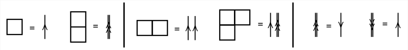
One can see that fundamental and anti-fundamental representations can be represented either by lines with a single arrow in one direction, or by lines with a double arrow in the opposite direction. More complex representations can be built by combining such lines together.
For lattices where vertices connect to more links, such as a square lattice in 2D or 3D, not all states that can be labeled by the representation above are linearly independent, leading to an ambiguity in labeling the basis states. This is due to the so-called Mandelstam constraints, which relate contractions of representation indices across a vertex. A point splitting procedure can be performed to split each vertex into three link vertices connected by virtual links, which lifts this ambiguity. In this point-split lattice, the gauge invariant states can be specified with the same assignment of labels used on a trivalent lattice.
There is an equivalent labeling of the states of the physical Hilbert space that will provide useful, using the arrow representation introduced above. This is illustrated in Fig. S2, and will be called a “loop representation”222Note that this presentation only works as presented in the simplest topological sector of the allowed states. There are other states that allow for additional overall winding numbers, which will not be considered in this work. One can easily generalize the loop representation to also include winding loops..
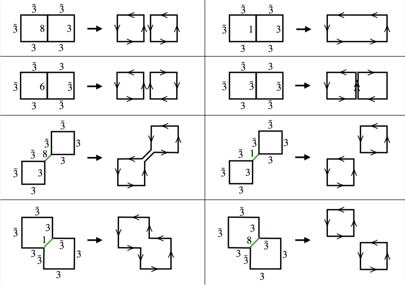
In this representation each state is labeled by a set of loops , together with a specification , which denotes the way the arrows at each link having more than one loop pass through being combined. Each loop needs to specify which plaquettes are encircled and in which order, while contains the information how to combine lines of multiple loops into single or double arrows. Note that it might seem that there is an ambiguity in the choice of single arrows in one or double arrows in the other direction. This ambiguity is fixed by choosing representations with or to have only single arrows, and demanding that the number of arrows entering and leaving a vertex is conserved. Due to the point splitting, closed loops have have the property that their lines can not cross each other, so they can not form knots or be twisted. A loop representation is therefore spanned by the states
| (S1) |
Note that this loop representation is simply a graphical representation of the states with definite representation at each link. In particular, lines do not necessarily represent the tensor indices of a given representation, and lines being connected does not necessarily imply tensor indices being contracted. Before moving on, we want to make it clear that the loop representation as given is likely not a computationally efficient representation of the Hilbert space, since loops are necessarily non-local objects which can in general span an arbitrary number of plaquettes. Its usefulness will come from when applying the expansion.
The vacuum state in the interacting theory can be generated adiabatically from the vacuum state of the free electric theory (the vacuum at ) by acting with the operators of the interacting Hamiltonian, which are operators at the different plaquettes or operators at the different links. Excited states in the simpliest topological sector can be obtained by further applications of electric energy or plaquette operators. One can therefore classify all states in this sector by the minimum number of plaquette operators and its conjugate that are required to reach it from the vacuum
| (S2) |
This state will be a linear combination of several basis states, one can write
| (S3) |
I.2 Scaling
The large scaling of a state, is determined by the large expansion of for the minimal choice of and to obtain a nonzero overlap. Using that the overlap is in the scaling, the scaling is therefore determined by the overlap . This overlap can be evaluated in the magnetic basis through inserting . To evaluate the large scaling of these integrals, the identity
| (S6) |
will be used [100]. The large scaling will be determined by the permutation of indices contraction that gives the largest factors of . A diagrammatic method of evaluating the large scaling is shown in Fig. S3.
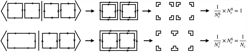
First, the plaquette operators being applied are placed over loops in the final state. To determine the powers of that come from contracting the Kronecker s, one can erase the middle of each link in the diagram and connect the lines from the same vertex. This leaves a set of closed loops involving one vertex each, and each of these closed loops contributes a factor of in the numerator. Each loop therefore contributes a factor and the the total scaling is given by
| (S7) |
to the final overlap. Since each in Eq. (S6) corresponds to a line in the figure, one immediately finds that , where is the total number of lines on each link in the diagram. Denoting by the number of plaquettes encircled by each loop , one needs plaquette operators for each loop. The total number of lines is then given by . Thus one finds
| (S8) |
The total number of closed loops is given by for each loop in the basis, such that one finds
| (S9) |
Putting this together, one finds that each loop contributes a factor of
| (S10) |
to the overall scaling of the overlap. This implies that the states that can be reached to leading order in are those that only involve loops with . Therefore, the only overlap that survives in the large limit is the one with states for which each loop encircles exactly one plaquette.
II Plaquette Matrix Elements
The plaquette matrix elements (introduced in [46]) can be conveniently represented on a point-split vertex where it will be expanded as a sum over generators of gauge-invariant rotations in the electric multiplet basis. While the generic expression depends on symbols formed by contractions of Clebsch-Gordan coefficients [45, 46], analytic expressions for matrix elements of low lying representations can be determined for arbitrary .
In the electric basis, the matrix elements of the link operator take the form
| (S11) |
where is the Clebsch-Gordan coefficient describing the combination of representations and into representation . Gauge invariant states in the theory will be formed from singlets at each vertex whose wavefunctions will be denoted by
| (S12) |
Using these singlet states, the gauge-invariant wavefunction for the plaquette in Fig. S4 can be written as
| (S13) |
Using Eq. (S11) and Eq. (S13), the matrix elements of the plaquette operator can be written as
| (S14) | ||||
| (S15) |
where the ’s are vertex factors defined by
| (S16) |
When the lattice is a 1D chain of plaquettes, this is sufficient to describe all plaquette matrix elements between gauge invariant states. In higher spatial dimensions, this result can still be used provided the theory is placed on a point-split lattice.
To evaluate vertex factors with arbitrary SU(N), a few general identities for the Clebsch-Gordan coefficients will be needed. If one of the lower entries of the Clebsh-Gordan coefficients is the singlet, then the coefficient is given by
| (S17) |
Also, if two representations are combining to form a singlet the only non-zero Clebsch-Gordan coefficients are given by
| (S18) |
Adding representations gives orthonormal states which gives the identity
| (S19) |
Another useful identity follows from multiple choices of decompositions of the singlet into three representations, i.e.
| (S20) |
implies
| (S21) |
Using these identities, we find
| (S22) |
For the truncations considered in this work, each plaquette is constrained to have a single loop of flux running around it. Generically, the matrix elements of plaquette operators only depends on the links on the plaquette and the electric flux flowing into each vertex of the plaquette. By considering Eq. (S15) on a point-split lattice, it can be seen that at this truncation in the plaquette basis, the matrix elements of a plaquette operator only depend on the plaquette being acted on and the plaquettes that share a link with it. Using Eq. (S15) and Eq. (S22), it can be seen that when the neighboring plaquettes are unexcited, the matrix elements for allowed transitions is always . Explicitly for , we have
| (S23) |
and specific to the case of
| (S24) |
When neighboring plaquettes are allowed to have a shared link in the representation given by anti-symmetric combination of fundamental representations, more matrix elements need to be considered. These can be evaluated using the above vertex factors and the fact that plaquette operators commute. For example, consider a chain of three plaquettes. Using Eq. (S15) and Eq. (S22), we find
| (S25) |
The matrix element can be evaluated in the same manner or by using the previous matrix element and the commutativity of plaquette operators. Explicitly, we have
| (S26) |
The same style of argument can be used on a square lattice to find
| (S27) |
where is the number of in the state . Note that this method can also be used to derive the non large suppressed plaquette matrix elements needed to include the and representations.
III Monte Carlo
For the truncated Hamiltonians studied in this work, static properties at finite temperature can be determined using Monte Carlo techniques. In general, the Boltzmann distribution can be approximated by
| (S28) |
By inserting a complete set of states, one can obtain a sum over states that can be sampled with the Metropolis algorithm. If all matrix elements of each of the are positive, then this sampling can be done without a sign problem.
Explicitly for the single loop Hamiltonian in the main text, the Boltzmann distribution can be approximated by
| (S29) |
where is the sum over all terms in the Hamiltonian that act on plaquettes on the even sublattice and is the sum over all terms in the Hamiltonian that act on plaquettes on the odd sublattice. Inserting a sum over electric basis states yields
| (S30) |
where the action is given by
| (S31) |
and is subject to the constraints that if all of its neighbors in the spatial directions are and for . is positive definite and therefore the sum over field configurations can be sampled with the Metropolis algorithm without a sign problem. Note that the derivation of this action is analogous to the relationship between the quantum Ising model and the classical Ising model in one higher dimension [155]. A similar decomposition can be done for the Hamiltonian including vertices with three incoming representations.
For the calculations in the main text, a spatial lattice with periodic boundary conditions was simulated at with imaginary time steps for various values of . For each coupling , samples of field configurations were generated with the Metropolis algorithm. The first field configurations of each sample were discarded and the remaining were used to compute observables. Error bars were computed through bootstrap resampling of the samples.
IV Quantum Simulation Implementation
IV.1 Interaction Picture Trotterization
The standard strategy for simulating time evolution in a lattice gauge theory has been to utilize a Trotterized time evolution operator where the time evolution generated by is approximated by
| (S32) |
The errors induced by Trotterizing into electric and magnetic terms will be . In an electric basis, the electric Hamiltonian, , is diagonal and can be implemented with single and controlled rotations. The magnetic Hamiltonian, , will generate rotations between different electric basis states and its implementation will generally require further Trotterization. The errors from this further Trotterization of the magnetic Hamiltonian will be . In the limit of strong coupling, the dominant source of error in the Trotterized time evolution will therefore come from the splitting into electric and magnetic terms.
This source of error can be reduced by instead performing the simulation in an interaction picture where the electric energy is taken to be the “free” term in the Hamiltonian. Explicitly, if we define , then the time evolution operator is given by
| (S33) |
By breaking up the time ordered matrix exponential into small time steps, it can be approximated by
| (S34) |
The size of the error in this approximation was estimated from the next to leading order term in the Magnus expansion. Therefore, by performing time evolution in the simulation in the interaction picture and Trotterizing into an implementable circuit, the error in a single time step will be , as desired. This is a factor of difference from the standard Trotterization in Eq. (S32) and will be helpful when performing simulations at large .
The quantum simulations of the single loop Hamiltonian presented in the main text were performed using this interaction picture Trotterization. Note that the magnetic term in this Hamiltonian contains a diagonal piece that will be absorbed into the electric Hamiltonian when going to the interaction picture. The interaction picture magnetic Hamiltonian is given by
| (S35) |
where labels a plaquette on the lattice, denotes the set of plaquettes neighboring and .
To Trotterize time evolution generated by this operator, the sum over plaquettes will be split into two separate sum over sublattices. Each plaquette on a lattice can be labeled by coordinates placed at the center of the plaquette. The lattice will be separated into an even sublattice, , and odd sublattice, , where the even sublattice contains all plaquettes with coordinates such that and the odd sublattice contains all remaining plaquettes. This separation is chosen such that all plaquettes in each sublattice commute with each other and when mapped to circuits can be implemented in parallel. With this decomposition, the time evolution operator can be Trotterized as
| (S36) |
where is the same as except the sum has been restricted to plaquettes in the even sublattice and is restricted to the odd sublattice.
IV.2 Time Evolution Circuits
Implementation of the Trotterized time evolution described in the previous section requires a mapping onto the qubits of a quantum computer and circuits that respects the computer’s connectivity. The Trotterized time evolution operator in Eq (S36), can be decomposed into
| (S37) |
for appropriately chosen and . A complication arises when implementing a circuit for or on IBM’s superconducting quantum processors as they do not have a square geometry [136]. However, a square lattice can be embedded on their heavy hex connectivity as shown in Fig. S5, where the blue lines denote the links on the 2 dimensional lattice. The circular qubits at the center of plaquettes are used to represent the state of the plaquette at that position. The remaining qubits on the chip will be used as ancillas to help implement these unitaries. To explain this better, we have color coded the qubits in Fig. S5 according to their role in the circuit. Circular qubits are used to represent the state of the system and square qubits are ancillas. Yellow qubits (blue) correspond to physical qubits on even (odd) lattice sites. Dark green square qubits denote the ancilla qubits on the left and right of the physical qubits storing the information about the four neighboring qubits for implementing controlled operations. Finally, light green qubits are used to communicate information between the dark green ancillas.
To implement the circuit, we recall that the magnetic component of the Hamiltonian given in equation (10) of the main text requires applying an gate to a plaquette if the neighboring plaquettes are in the zero state. The strategy used to implement these unitaries on a sublattice will be to store the information about neighboring plaquettes in the two ancilla qubits located adjacent to the physical qubit being evolved. To be explicit, the ancilla qubits – will be put in the state if both of the neighboring plaquettes and it represents are in the state, and left in the state otherwise. This is essentially an implementation of the standard technique to implement multi-control gates using ancilla qubits on the geometry of ibm_torino [156]. The explicit circuit to prepare the ancilla qubits is shown in Fig. S6.
Using this circuit, can be implemented by applying the ancilla preparation circuit to the neighboring ancillas, applying (where and are the ancillas neighboring qubit ), and then undoing the ancilla preparation circuit. Note that each qubit in the even (or odd) sublattice will require the same set of ancillas to be prepared. Therefore, one can apply the ancilla preparation to all ancillas on the lattice, evolve the entire sublattice in parallel and then undo the ancilla preparation circuits. To be more explicit, a classification of the qubits on ibm_torino is shown in Fig. S5. Qubits on the even sublattice are shown in yellow and qubits on the odd sublattice are shown in blue. To evolve the qubits on the even sublattice, the ancilla preparation circuit would be applied to each line of ancilla qubits between the blue qubits. Then, the yellow qubits are evolved with controls from the green qubits. The ancilla circuits are then undone before evolving the other sublattice. By also alternating the order in which the even and odd lattices are evolved, i.e. in one step evolve even then odd and in the next step evolve odd then even, half of the ancilla circuits can be cancelled. This results in a CNOT depth of 45 per Trotter step (and a depth of 23 for the first Trotter step by cancelling CNOT gates against the initial state).
@C=1em @R=1em
\lstickP_1 &\ctrl1 \qw \qw \qw \qw \qw \qw \qw \qw\ctrl1 \qw\qw\qw
\lstickA_1 \targ\qw \qw \qw \ctrl1 \qw \qw \qw \ctrl1 \targ\targ\qw\qw
\lstickA_2 \gateH \gatee^-iπ8^Z\targ\gatee^-iπ8^Z\targ \gatee^-iπ8^Z \targ \gatee^-iπ8^Z \targ\gateH\ctrl-1\ctrl1 \qw
\lstickA_3 \targ\qw \ctrl-1 \qw \qw \qw \ctrl-1 \qw \qw\targ\qw\targ\qw
\lstickP_2 \ctrl-1\qw \qw \qw \qw \qw \qw \qw \qw\ctrl-1 \qw\qw\qw
IV.3 Error Mitigation
Current quantum hardware suffers from noise and gate errors that limit the accuracy of simulations. These errors can be reduced using error suppression and error mitigation techniques. In this work, dynamical decoupling with an sequence was used to reduce the coherent errors in the calculation [137]. Pauli twirling was applied to all CNOT gates in the circuit to convert all coherent noise into Pauli error channels [138, 50, 48]. These error suppression techniques reduce the size of errors in the calculation, but do not correct them. Measurement errors in the calculation were mitigated using Twirled Readout EXtincation (T-REX) mitigation [144]. In this technique, a Pauli operator is applied at the end of the circuit and the change in sign of the measured operator is corrected in post processing. If the incoherent noise in the circuit can be modelled by a Pauli error channel following the correct circuit, the errors in Pauli operators can be corrected using Operator Decoherence Renormalization (ODR) [138, 50, 48, 77]. In ODR, two circuits are run on the hardware, a “physics” and a “mitigation” circuit. The mitigation circuit is chosen such that it can be simulated classically. For the simulation in this work, the physics circuit is the Trotterized time evolution circuit described above, and the mitigation circuit is the same circuit except with . Under the assumption that the incoherent noise in the circuit can be modelled by a Pauli error channel following the correct circuit, the measured Pauli operator is proportional to the value that would be measured in the absence of noise. The constant of proportionality can be determined using the mitigation circuit, because the noiseless value can be computed classically, and used to correct the results of the physics circuit. This can significantly reduce the effect of noise but does not correct all errors because not all noise can be modelled this way. The dominant source of error in the computation comes from the CNOT gates. In the absence of noise, replacing a CNOT gate with a sequence of three CNOT gates would not change the circuit. In reality, this enhances the amount of noise in the circuit. By probabilistically inserting pairs of CNOT gates, the noise in the circuit can be amplified by a continuous parameter . This can then be used to extrapolate to the zero noise limit [138, 142, 143]. In this work, CNOT gates were replaced by three CNOT gates with probability which corresponds to . Both the and circuits were mitigated using ODR and T-REX before performing a linear extrapolation to the zero noise limit.
To test the effectiveness of these error mitigation techniques for the simulations in this work, the single loop Hamiltonian in the main text was simulated on a lattice with plaquettes with open boundary condititions and . The time evolution circuit described in the previous section was used to evolve the electric vacuum and was implemented using . For a lattice of this size, 16 qubits are needed to represent the state of the system, and on ibm_torino a 39 qubit block was used due to the connectivity constraints of the hardware. For each time slice, different Pauli twirls were used for physics and mitigation circuits for both and . In each separate twirl, CNOT gates were inserted probabilistically. Each individual circuit was evaluated with shots. The probability of a plaquette being excited averaged over the lattice as a function of time is shown in Fig. S7. In these simulations, the probability of each qubit being excited was individually mitigated before being averaged over the lattice. This figure shows that the error mitigation procedure used in this work can be used to reliably implement up to Trotter steps.
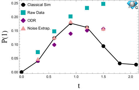
In addition to the errors from imperfect hardware, the quantum simulation performed on ibm_torino has errors from the Trotterization of the time evolution operator. These errors can be mitigated by performing simulations with different time steps, , that sample the same points in time. For each point in time that is sampled by multiple , a linear extrapolation to can be performed. Fig. S8 shows the values of that were sampled in the plaquette lattice simulation on ibm_torino. The green points indicate the results of the extrapolation in . The circled points at each indicate the point with the smallest theoretical error at that . For times that were sampled by multiple , this would be the value obtained by the extrapolation and for points sampled only once that would be the result of the error mitigation described in the previous paragraph. Fig. S9 shows the same data for the plaquette lattice simulation. Note that because statevector simulation of systems of this size are beyond what can be done with classical computers, the classical simulations in this figure were performed with tensor networks. The tensor network simulations were performed using CuQuantum [152] on a single NVIDIA A100 GPU.