Radiative-Conductive Heat Transfer Dynamics in Dissipative Dispersive Anisotropic Media

Abstract

We develop a self-consistent theoretical formalism to model the dynamics of heat transfer in dissipative, dispersive, anisotropic nanoscale media, such as metamaterials. We employ our envelope dyadic Green’s function method to solve Maxwell’s macroscopic equations for the propagation of fluctuating electromagnetic fields in the media. We assume that the photonic radiative heat transfer mechanism in the media is complemented by phononic mechanisms of heat storage and conduction, accounting for effects of local heat generation and material phase transitions. By employing the Poynting theorem and the fluctuation-dissipation theorem, we derive novel closed-form expressions for the coupling term of photonic and phononic subsystems, which contains the heating rate and the radiative heat power terms, as well as for the radiative heat flux. We apply our formalism to the paraxial heat transfer in uniaxial media and present relevant closed-form expressions. By considering a Gaussian transverse temperature profile, we also obtain and solve the integro-differential heat diffusion equations to model the paraxial heat transfer in uniaxial reciprocal media.

• January 2024

Keywords: dynamics of radiative heat transfer, radiative heat flux, temperature profile, dissipative media, metamaterials, nanowires

1 Introduction

It is well-known that the heat transfer (HT) in media is mediated by two main mechanisms: photonic, the radiative heat transfer (RHT), and phononic, the thermal conduction. The RHT is associated with the fluctuating electromagnetic fields (FEFs) which are produced by thermally agitated random motions of electric charges in the medium while the thermal conduction is associated with collective oscillations of atoms in a lattice. The phononic mechanism comprises the thermal heat conduction and storage, which has been known for a long time (e.g., cf. [1]). The RHT is governed by the fluctuation-dissipation theorem (FDT) and Rytov’s fluctuational electrodynamics [2]. It has been also theoretically and experimentally shown [3, 4, 5, 6, 7, 8, 9, 10, 11] that the radiative heat exchange becomes dominating when separation between objects is decreased. While the far-field RHT for two separated objects is limited by the Planck’s blackbody radiation law, the RHT in the near field can increase by orders of magnitude above the blackbody radiation limit when the separation becomes deeply sub-wavelength. For such case, it is necessary to consider the near-filed radiative heat transfer (NFRHT) [12] since near-field effects, i.e. the collective influence of diffraction, interference, and tunneling of waves, become important [13]. Hence, the Planck’s blackbody radiation law and the Stefan-Boltzmann law are no longer valid to determine the spectral emissivity and total emissive power when object’s geometric dimensions are comparable to the characteristic wavelength of thermal radiation.

Nowadays, there is a growing interest in the study of NFRHT in the micro- and nano-scale objects, especially, metamaterials (MMs). Due to their peculiar properties, MMs are increasingly adopted in many scientific and technological applications [14, 15, 16, 17, 18, 19, 20, 21, 22, 23, 24, 25, 26, 27, 28, 29, 30, 31, 32, 33]. Recently, the super Planckian NFRHT has attracted attention of science and technology [34, 35, 36, 37, 38, 39, 40, 41] with applications in thermionic systems, thermophotovoltaics, energy harvesting, local thermal control and management, thermal modulation, nanoscale infrared imaging and mapping, and nanomanufacturing. This development has been complemented by studies of thermal properties of MMs [42, 43, 44, 45, 46, 47, 48, 49, 50, 51]. Moreover, further extent of nanoscale RHT studies into multidisciplinary areas may assist in solving current societal challenge. For instance, regarding the increasing dangers of global warming, new MMs have been proposed for applications in thermophotovoltaics systems that can efficiently convert thermal energy from any kind of heat source into electricity [52] or perform radiative cooling under direct sunlight, aiming to reduce global energy consumption [53]. All-dielectric MMs for similar energy harvesting applications have been designed by using Machine Learning techniques [54]. It is worth to mention that control of thermal flux by utilizing photonic devices becomes increasingly attractive because of applications of such devices as thermal diodes and thermal logic gates, and even as thermal cloaks [46, 55, 56, 57, 58]. Another actively developing area is the microfluidic and nanofluidic thermal management for electronic devices [59, 60]. All these observations highlight the necessity of paying attention to the mechanisms of combined conductive-radiative HT in nanoscale media such as MMs.

Although many important theoretical methods have been proposed to analyze the heat diffusion in MMs based on the fluctuational electrodynamics and the microscopic/ macroscopic Maxwell equations, [3, 4, 5, 6, 7, 8, 26, 31, 61, 62, 63, 64], there is not much theoretical work specifically devoted to modeling the dynamics of HT (DHT) in nanoscale media. Recently, in the framework of the slowly varying amplitude (SVA) approach, we presented a novel method, namely, the envelope dyadic Green’s function (EDGF) [65], which is different from the standard dyadic Green’s function method. With this method, one can obtain the propagating fluctuating electromagnetic fields in dispersive anisotropic media by using the precalculated EDGFs for the uniaxial MMs.

In this paper, based on our EDGF method [65], we aim to develop a self-consistent theoretical formalism to model the DHT in dissipative dispersive anisotropic nanoscale media (DDANM) such as MMs, with dyadic constitutive parameters such as the permittivity and the permeability. The formalism presented in this article neglects magneto-electric interactions that exist in bianisotropic media, however, it can be extended to include bianisotropic effects [66].

In what follows, assuming that the photonic HT mechanisms are complemented by dynamic phononic mechanisms of heat storage and conduction, we shall present closed form relations for the coupling term of the photonic-phononic HT mechanisms, expressed in terms of the heating rate and the power of radiative heat flux. As we mentioned above, these relations are obtained using our EDGF method by employing the Poynting and FDT theorems, while accounting for the effects of local heating and the material phase transitions. At the next step, we apply our formalism to paraxial propagation in uniaxial media such as one-dimensional crystalls of nanolayers with an aim to solve the heat diffusion equations in such media. To do this, we express the transverse temperature profile as a superposition of multiplicative terms comprising Gaussian and polynomial functions and present a group of integro-differential equations for the temperature distribution in the axial direction. Then, the formulated equations can be discretized and solved.

This article is organized as follows: In Section 1, we explain the fundamental concepts in the context of heat transfer and present relevant formulas. In Section 2, by considering the propagation of fluctuating electromagnetic fields with SVAs (FEFSVAs) in DDANM, we construct a self-consistent DHT formalism and obtain closed-form expressions for the heating rate, the radiative power, and the radiative heat flux. In Section 3, we shall apply our DHT formalism for the propagation of paraxial FEFSVAs in a DDAN uniaxial medium. In Section 4, we obtain integro-differential equations for the heat diffusion in a reciprocal medium. Finally, in Section 5, we discuss the obtained results and make conclusions.

2 HEAT TRANSFER

In the modeling of DHT in DDANM, the key unknown is the temperature distribution that must be extracted from the heat diffusion equation in the medium which, obviously, combines both phononic and photonic HT mechanisms. Thermally-agitated noise in the form of FEF is produced by random motions of charge carriers and vibrations of polarized atoms in the medium. In turn, FEF when propagating in a lossy medium, dissipates electromagnetic energy into the heat in the form of similar random vibrations. Thus, random phononic processes in a material with loss are coupled to random photonic processes and vice versa.

The phononic mechanism mentioned above comprises the heat conduction and storage due to the processes such as lattice vibrations, material phase transitions, etc. In this section, we consider the effective thermal conduction of the materials and the latent heat associated with such processes. On the other hand, in regard to the photonic HT, here we need to calculate the generated heat term which must occur in the heat diffusion equation.

The equation for the heat diffusion due to phonons in a medium kept under constant volume can be constructed phenomenologically, by balancing the growth rate of the phononic thermal energy per unit volume, $dU_{V}/dt$, with the rates of heat supply, $dQ^{s}_{V}/dt$, and release, $dQ^{r}_{V}/dt$, per unit volume, as follows:

$${dU_{V}\over dt}={dQ^{s}_{V}\over dt}-{dQ^{r}_{V}\over dt}.$$ (1)

As is well-known from thermodynamics, a variation of the thermal energy of the medium under isochoric conditions can be expressed through its temperature variation, $dT$, the specific heat capacity of the material at constant volume, $c_{v}(T)$, and the variation of the latent heat, $dL_{p}$, associated with material phase transitions. Here we consider only the processes in which the change of material mass density $\varrho_{m}$ is either naturally negligible (such as ferromagnetic-paramagnetic transitions, etc.) or vanishes due to the enforced isochoric conditions. Thus, we have

$$dU_{V}=\varrho_{m}c_{v}(T)dT+dL_{p},$$ (2)

During a phase transition that happens at the transition temperature $T=T_{p}$, the material temperature stays constant and thus $dT=0$, while $dL_{p}\neq 0$. When $T\neq T_{p}$, $dLp=0$. At the point $T=T_{p}$, the specific heat capacity $c_{v}(T)$ can be discontinuous, because $c_{v}$ can differ for the two phases.

In order to calculate the rate of heat supply that drives the phononic HT subsystem, we need to consider the heating rate density due to the passing radiation, $h^{\Sigma}_{EM}$, where the label ^Σ means that contributions from FEFs with all possible frequencies are taken into account, and the density of the generated heat from other sources, $g_{c}$, which can be chemical processes, etc. Thus, the heat supply rate per volume of the medium reads

$${dQ_{V}^{s}\over dt}=h_{EM}^{\Sigma}+g_{c}.$$ (3)

In order to find the heat release rate, we have to consider the phononic heat density, $\vec{q}_{c}$, and the power density of locally generated thermal radiation, $p^{\Sigma}_{rad}$:

$${dQ_{V}^{r}\over dt}=\nabla\cdot\vec{q}_{c}+p^{\Sigma}_{rad},$$ (4)

where $\vec{q}_{c}=\overline{\overline{\alpha}}_{c}\cdot\nabla T$, with $\overline{\overline{\alpha}}_{c}$ as the phononic thermal conductivity tensor of the medium.

The heat diffusion equation associated with phononic processes can be written as follows:

$$\varrho_{m}c_{v}(T){dT\over dt}+{dL_{p}\over dt}=-\nabla\cdot({\overline{\overline{\alpha}}_{c}\cdot\nabla T})+g_{c}+(h_{EM}^{\Sigma}-p^{\Sigma}_{rad}),$$ (5)

In order to quantify the coupling term $(h_{EM}^{\Sigma}-p^{\Sigma}_{rad})$ at every carrier frequency $\omega$, the heating rate density, $h_{EM}^{\Sigma}(\omega)$, and the power density of locally generated thermal radiation, $p^{\Sigma}_{rad}(\omega)$, must be obtained based on the FDT and the electromagnetic properties of the material. In addition, for computing the total RHT rate, which is the first term in the right-hand side of Eq. (5), we need to calculate the radiative heat flux density associated with the FEF at the same frequency, $\vec{q}_{rad}(\omega)$. We postpone quantifying these terms untill Section 2, however, we point out the main physical concepts in the contexts involving conversion of the radiation energy into work and vice versa based on the microscopic and macroscopic views of the modeling of DHT in DDANM.

In the microscopic view, we need principally to consider the free energy of the system (involving FEFs) which is a fair thermodynamic potential comparing to the total energy. Free energy, as a measure of work that a system can do at constant temperature, contains the disordering in the system through including entropy and is calculated by the difference between the change in total energy and the energy lost in the form of heat. Given the photonic states density and the photonic distribution function (Bose-Einstein relation) with the known chemical potential of radiation (through the relationship with the chemical potentials of carriers), we can obtain the entropy of radiation in order to calculate the free energy for both equilibrium and non-equilibrium cases [67]. However, we postpone this microscopic view to a future work and, in following, we proceed with a macroscopic view, indeed, we consider only the average quadratic of thermal FEFs, total energy, and energy flux.

In order to model the DHT in DDANM macroscopically, we employ the Poynting’s theorem for FEFs, which gives the work done by these fields in the medium. In other words, we assume that the heating rate density, $h_{EM}$, in the presence of FEFs can be determined from the Poynting’s theorem for macroscopic electromagnetic fields and the material relations for such fields, in the same way as for non-stochastic electromagnetic processes (for the stochastic heat diffusion study, see, e.g., [68]). For this assumption to hold, the characteristic spatial scale of phononic thermal fluctuations generated by the dissipative processes (e.g., electron and phonon scattering on impurities, etc.) must be much smaller than that of the electromagnetic fluctuations, which is a reasonable assumption when considering macroscopic electromagnetic fields.

In order to obtain the coupling term and heat flux in the framework of the Poynting’s theorem, we need to calculate the work done by FEFs, $\vec{F}^{\,\alpha}=\vec{F}^{\,\alpha}_{0}\cos(\omega t+\phi_{\alpha})$, where $\phi_{\alpha}$ is an arbitrary phase with $\alpha=e,m$. Since in what follows we intend to work with the oscillating fields whose amplitudes and phases fluctuate, it is more convenient to write the electric and magnetic fields as $\vec{F}^{\,\alpha}=\mathfrak{R}\left(\vec{F}^{\,\alpha}_{m}e^{-i\omega t}\right)$, where $\vec{F}^{\,\alpha}_{m}$ are the time-dependent complex phasors of the fluctuating electric and magnetic fields and $\mathfrak{R}(\cdot)$ denotes the real part of a complex quantity. Moreover, $\vec{F}^{\,e}$ and $\vec{F}^{\,m}$, the fluctuating electric and magnetic fields, respectively, are related to the fluctuating electric and magnetic induction vectors, $\vec{\Xi}^{\,e}$ and $\vec{\Xi}^{\,m}$, respectively, through the constitutive relations of the form

$$\vec{\Xi}^{\,\alpha}=\overline{\overline{\zeta}}\,^{\alpha}\cdot\vec{F}^{\,\alpha},\qquad\alpha=e,m$$ (6)

where the dyadics $\overline{\overline{\zeta}}\,^{e}$ and $\overline{\overline{\zeta}}\,^{m}$ are, respectively, the absolute permittivity, $\overline{\overline{\varepsilon}}$, and absolute permeability, $\overline{\overline{\mu}}$, of the medium. When dealing with time-dependent fields in dispersive media, $\overline{\overline{\zeta}}\,^{\alpha}$ can be considered as a dyadic integro-differential operator. It should be noted that the complex field phasors, $\vec{F}^{\,e}_{m}$, $\vec{F}^{\,m}_{m}$, $\vec{\Xi}^{\,e}_{m}$, and $\vec{\Xi}^{\,m}_{m}$, also satisfy the frequency-domain Maxwell equations of the following form

$$\nabla\cdot\vec{\Xi}^{\,e[m]}_{m}=\rho_{m}^{e[m]},\qquad\nabla\times\vec{F}^{\,e[m]}_{m}=-[+]\left((\partial_{t}-i\omega)\vec{\Xi}^{\,m[e]}_{m}+\vec{J}_{m}^{\,m[e]}\right),$$ (7)

where $\vec{J}_{m}^{\,e[m]}$ is the complex amplitude of the electric (magnetic) current density, $\vec{J}^{\,e[m]}$. By keeping the time derivative of the complex field amplitudes, $\partial_{t}\Xi_{m}$, in the above equations, we emphasize that these quantities may vary with time as we expect in the fluctuating fields case.

The work $W_{EM}$ of embedded electric and magnetic current sources on exciting such random time-harmonic fields (per a period of oscillations) reads

$${\omega W_{EM}\over 2\pi} =\left\langle\int P_{src}dV\,\right\rangle_{T}$$

$$=\left\langle\int\left[\nabla\cdot\vec{S}+{1\over 2}(\vec{F}^{\,e}\cdot\partial_{t}\vec{\Xi}^{\,e}+\vec{F}^{\,m}\cdot\partial_{t}\vec{\Xi}^{\,m})\right]dV\right\rangle_{T},$$ (8)

where $\langle\ldots\rangle_{T}$ denotes averaging over a period of oscillations, $\partial_{t}={\partial\over\partial t}$, and $P_{src}$, the source power density, is defined by

$$\left\langle P_{src}\right\rangle_{T}=-\left\langle\vec{F}^{\,e}\cdot\vec{J}^{\,e\,*}+\vec{F}^{\,m\,*}\cdot\vec{J}^{\,m}\right\rangle_{T}=-{1\over 2}\mathfrak{R}\!\left[\vec{F}^{\,e}_{m}\cdot\vec{J}_{m}^{\,e\,*}+\vec{F}^{\,m\,*}_{m}\cdot\vec{J}_{m}^{\,m}\right],$$ (9)

On the right-hand side of Eq. (2), the Poynting vector $\vec{S}$ that appears in the first term is given by

$$\left\langle\vec{S}\,\right\rangle_{T}=\left\langle\vec{F}^{\,e}\times\vec{F}^{\,m}\right\rangle_{T}={1\over 2}\mathfrak{R}\!\left(\vec{F}^{\,e}_{m}\times\vec{F}^{\,m\,*}_{m}\right).$$ (10)

and the second term of the same expression is the total rate of the electromagnetic energy dissipation and storage per unit volume of the medium, which can be written in terms of the phasors as

$$q_{{}_{EM}}={1\over 2}\mathfrak{R}\!\left[\vec{F}^{\,e}_{m}\cdot(\partial_{t}+i\omega)\vec{\Xi}^{\,e\,*}_{m}+\vec{F}^{\,m\,*}_{m}\cdot(\partial_{t}-i\omega)\vec{\Xi}^{\,m}_{m}\right].$$ (11)

In Eqs. (2-11), we need to know the FEFs in the DDANM with known material parameters. In this work, we use our EDGF method [65] to solve the Maxwell macroscopic equations, Eq. (7).

In the EDGF formalism, we consider two main assumptions:

1. The time-harmonic FEFs $\vec{F}^{\alpha}_{m}$, flux densities $\vec{\Xi}^{\alpha}_{m}$, and currents $\vec{J}^{\alpha}_{m}$ are complex SVAs [65]:

   $$\vec{f}(t) ={1\over 2}\vec{f}_{m}(t)e^{-i\omega_{0}t}+c.c.,$$ (12)

   $$\vec{f}_{m}(t) ={1\over\pi}\int\limits_{-\Delta\omega/2}^{\Delta\omega/2}\vec{f}(\omega_{0}+\Omega)e^{-i\Omega t}d\Omega,\qquad f=F,\Xi,J,$$

   where $c.c.$ stands for the complex conjugate of the previous term, $\Omega=\omega-\omega_{0}$ with $\omega_{0}$ as the carrier frequency and $\Delta\omega\ll\omega_{0}$.

2. The frequency-dependent material dyadics $\overline{\overline{\zeta}}\,^{\alpha}(\omega)$ [the permittivity $\overline{\overline{\varepsilon}}(\omega)$ or the permeability $\overline{\overline{\mu}}(\omega)$] behave smoothly near $\omega_{0}$, so that we can expand $\overline{\overline{\zeta}}\,^{\alpha}$ around $\omega_{0}$ as follows

   $$\overline{\overline{\zeta}}\,^{\alpha}(\omega)=\overline{\overline{\zeta}}\,^{\alpha}_{{}_{\omega_{0}}}+(\partial_{\omega}\overline{\overline{\zeta}}\,^{\alpha})_{{}_{\omega_{0}}}\Omega+o(\Omega),$$ (13)

   where the subscript $\omega_{0}$ emphasizes that the quantity has to be calculated at $\omega_{0}$ (we keep this notation in the rest of this paper).

Based on these assumptions, we obtain a relation (which will be used in the next section) between the complex SVAs of the fluctuating electromagnetic fields and flux densities. Regarding Eqs. (6) and (12), we have

$$\vec{\Xi}^{\,\alpha}_{m}(t)={1\over\pi}\!\!\int\limits_{-\Delta\omega/2}^{\Delta\omega/2}\!\!\overline{\overline{\zeta}}\,^{\alpha}(\omega_{0}+\Omega)\cdot\vec{F}^{\,\alpha}_{m}(\omega_{0}+\Omega)e^{-i\Omega t}d\Omega.$$ (14)

Now, using Eqs. (12-13) and keeping only the first-order term of the Taylor’s expansion over $\Omega$, we obtain

$$\vec{\Xi}^{\,\alpha}_{m}(t)=\overline{\overline{\zeta}}\,^{\alpha}\cdot\vec{F}^{\,\alpha}_{m}+(\partial_{\omega}\overline{\overline{\zeta}}\,^{\alpha})_{{}_{\omega_{0}}}\!\!\cdot\left[{1\over\pi}\!\!\int\limits_{-\Delta\omega/2}^{\Delta\omega/2}\!\!\!\Omega\,\vec{F}^{\,\alpha}_{m}(\omega_{0}+\Omega)e^{-i\Omega t}d\Omega\right],$$ (15)

where the bracket in the second term of the right-hand side of Eq. (15) is the time derivative of $\vec{F}^{\,\alpha}_{m}(t)$ divided by a factor of $-i$. Thus, we find the following useful relation between the complex SVAs of the fluctuating electromagnetic fields and flux densities

$$\vec{\Xi}^{\,\alpha}_{m}(t)=\left[\overline{\overline{\zeta}}\,^{\alpha}+(\partial_{\omega}\overline{\overline{\zeta}}\,^{\alpha})(i\partial_{t})\right]_{{}_{\omega_{0}}}\!\!\cdot\vec{F}^{\,\alpha}_{m},\qquad\alpha=e\ \mbox{or}\ m.$$ (16)

Let us introduce the 6-vector electromagnetic fields and currents as follows:

$$\vec{\bf{F}}_{m}=\begin{bmatrix}\vec{F}^{\,e}_{m}\\ \vec{F}^{\,m}_{m}\end{bmatrix},\qquad\vec{\bf{J}}_{m}=\begin{bmatrix}\vec{J}^{\,e}_{m}\\ \vec{J}^{\,m}_{m}\end{bmatrix}.$$ (17)

$\vec{\bf{F}}_{m}$ is given by the following operator form [65]:

$$\vec{\bf{F}}_{m}=\hat{\overline{\overline{\bf{G}}}}\cdot\vec{\bf{J}}_{m},$$ (18)

which is understood as the following integral

$$\vec{\bf{F}}_{m}\left(\vec{r},t\right)=\int\overline{\overline{\bf{G}}}(\vec{r},t;\vec{r}^{\,\prime},t^{\prime})\cdot\vec{\bf{J}}_{m}(\vec{r}^{\,\prime},t^{\prime})d^{3}r^{\,\prime}dt^{\prime},$$ (19)

where $\overline{\overline{\bf{G}}}$ is EDGF.

To model DHT, in addition to the extracted FEFs from the EDGF and the Poynting theorem, we use FDT which states that the fluctuation properties of a system in thermal equilibrium can be expressed in terms of the linear response of the same system to an external perturbation [2]. According to the FDT, for an anisotropic local medium at local thermal equilibrium, the correlation function of thermally generated random currents reads

$$\left\langle\vec{J}_{\omega}^{\,\alpha}(\vec{r},\omega)\vec{J}_{\omega}^{\,\alpha}\,{}^{*}(\vec{r}^{\,\prime},\omega^{\,\prime})\right\rangle={4\Theta(\omega,T)\over\pi}\mathfrak{I}(\overline{\overline{\zeta}}\,^{\alpha}_{\omega})\,\delta(\omega-\omega^{\prime})\delta(\vec{r}-\vec{r}^{\,\prime}),$$ (20)

where $\vec{J}_{\omega}^{\,\alpha}$ is the time-harmonic fluctuating (electric or magnetic) current density, $\Theta(\omega,T)=\hbar\omega(e^{\hbar\omega/k_{B}T}-1)^{-1}$ is the mean Planck’s oscillator energy as a function of frequency and temperature and $\mathfrak{I}(\overline{\overline{\zeta}}\,^{\alpha}_{\omega})$ the imaginary part of the Fourier transform of $\overline{\overline{\zeta}}\,^{\alpha}$.

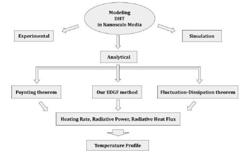
Figure 1: A chart illustrating the position of current work among other known DHT modeling approaches.

We conclude this section with a graphical illustration that clarifies positioning of our method of modeling of the heat transfer dynamics in DDANM with respect to other known methods. According to the literature, there are three main approaches, namely, experimental, analytical, and numerical simulation, to do this. As presented by the central path of the flowchart shown in Fig.  (1), the analytical model of DHT in such media developed in our work is founded on the three pillars: The Poynting theorem, FDT, and the EDGF method, which allow us to simultaneously characterize the heating rate, radiative power, and radiative heat flux, and, with that information, obtain the resulting temperature distribution within the material, as will be shown in the following sections.

3 Heating rate, radiative power, and radiative heat flux

In this section, in the framework of the EDGF method [65] and employing the Poynting theorem and FDT, we obtain closed-form expressions for $h_{EM}$, $p_{rad}$, and $\vec{q}_{rad}$, at an arbitrary point in the radiation frequency spectrum, $\omega_{0}$, which we call the carrier frequency. Next, by integrating over all carrier frequencies we obtain the total heating rate $h_{EM}^{\,\Sigma}$, the total radiative power $p_{rad}^{\,\Sigma}$, and the total radiative heat flux $\vec{q}_{rad}^{\,\Sigma}$. It should be noted that we shall calculate the Poynting vector of FEFSVA as a function of carrier frequency ($\omega_{0}$), position, and time for an arbitrary plane inside a medium by obtaining the component of the Poynting vector perpendicular to the plane. Thus, with the yielded quantity it will be possible to describe the RHT in the DDANM with non-uniform distribution of temperature. It is worth to mention that when employing FDT, which allows us to relate the ensemble average of the square of fluctuating electric (magnetic) current density to the Planck’s oscillator energy and the imaginary part of the permittivity (permeability) tensor, we assume that there is no correlation between the electric and magnetic components of the fluctuating current density.

In order to calculate the heating rate density, the coupling term, $h_{EM}^{\Sigma}-p_{rad}^{\Sigma}$, and the heat flux, $\vec{q}_{rad}^{\,\Sigma}$, by use of the FDT, let us have a closer look at Eq. (11):

$$q_{{}_{EM}}={1\over 2}\mathfrak{R}\!\left[\vec{F}^{\,e}_{m}\cdot(\partial_{t}+i\omega)\vec{\Xi}^{\,e\,*}_{m}+\vec{F}^{\,m\,*}_{m}\cdot(\partial_{t}-i\omega)\vec{\Xi}^{\,m}_{m}\right].$$

We claim that the right-hand side of this equation is a sum of the dissipation power (i.e. the rate of transformation of the electromagnetic energy into heat) and the rate of electromagnetic energy storage in a unit volume of the medium. Separation of these contributions into two explicit terms is possible only in very special cases. On the other hand, for truly monochromatic processes, there is no energy storage on average, and thus this term is entirely dissipative. Likewise, for the processes with finite duration in which the field amplitude first gradually increases from zero to some value and then decreases back to zero, the integral

$$Q_{EM} ={1\over 2}\mathfrak{R}\!\int\limits_{-\infty}^{\infty}\left[\vec{F}^{\,e}_{m}\cdot(\partial_{t}+i\omega)\vec{\Xi}^{\,e\,*}_{m}+\vec{F}^{\,m\,*}_{m}\cdot(\partial_{t}-i\omega)\vec{\Xi}^{\,m}_{m}\right]_{{}_{\omega_{0}}}\!\!\!dt$$

$$\equiv Q^{e}_{EM}+Q^{m}_{EM},$$ (21)

has the meaning of the total heat produced by the dissipative processes per unit volume of the material. Let us find a closed-form expression for $Q^{e}_{EM}$. Using Eq. (16), we can write the right-hand side of Eq. (3) as $Q^{\,e}_{EM}\equiv Q^{\,e}_{EM,\,1}+Q^{\,e}_{EM,\,2}$, where

$$Q^{\,e}_{EM,\,1}={1\over 2}\mathfrak{R}\!\int\limits_{-\infty}^{\infty}\partial_{t}\left[\left(\overline{\overline{\zeta}}\,^{e}+\partial_{\omega}\overline{\overline{\zeta}}\,^{e}i\partial_{t}\right)_{{}_{\omega_{0}}}\cdot\vec{F}_{m}^{e}\right]^{\dagger}\cdot\vec{F}_{m}^{e}\,dt$$ (22)

$$Q^{\,e}_{EM,\,2}={1\over 2}\mathfrak{R}\!\int\limits_{-\infty}^{\infty}(i\omega_{0})\left[\left(\overline{\overline{\zeta}}\,^{e}+\partial_{\omega}\overline{\overline{\zeta}}\,^{e}i\partial_{t}\right)_{{}_{\omega_{0}}}\cdot\vec{F}_{m}^{e}\right]^{\dagger}\cdot\vec{F}_{m}^{e}\,dt$$

By ignoring the terms on the order of $O(\partial^{2}_{t})$ and separating the material dyadic operator $\overline{\overline{\zeta}}\,^{e}=\overline{\overline{\zeta}}\,^{\prime\,e}+i\overline{\overline{\zeta}}\,^{\prime\prime\,e}$ into the Hermitian and anti-Hermitian parts, $\overline{\overline{\zeta}}\,^{\prime\,e}$ and $i\overline{\overline{\zeta}}\,^{\prime\prime\,e}$, respectively, one can easily verify that $\mathfrak{R}\int_{-\infty}^{\infty}\vec{F}^{e\,\dagger}_{m}\cdot(\overline{\overline{\zeta}}\,^{\prime\,e}\partial_{t})\cdot\vec{F}_{m}^{e}\,dt=0$ since $\partial^{\dagger}_{t}=-\partial_{t}$ and then

$$Q^{\,e}_{EM,\,1}={1\over 2}\int\limits_{-\infty}^{\infty}\vec{F}_{m}^{\,e\dagger}\cdot(\overline{\overline{\zeta}}\,^{\prime\prime\,e}_{{}_{\omega_{0}}}i\partial_{t})\cdot\vec{F}_{m}^{e}\,dt.$$ (23)

In the above equation, at the last step, we used the fact that $\int\limits_{-\infty}^{\infty}i\partial_{t}\left(\vec{F}_{m}^{\,e\dagger}\cdot\overline{\overline{\zeta}}\,^{\prime\prime\,e}_{{}_{\omega_{0}}}\cdot\vec{F}_{m}^{e}\right)\,dt=0$. Now, we can decompose $Q^{e}_{EM,\,2}$ in two terms as follows

$$Q^{\,e}_{EM,\,2}= {1\over 2}\mathfrak{R}\int\limits_{-\infty}^{\infty}(i\omega_{0})\left[(\overline{\overline{\zeta}}\,^{\prime\,e}+i\overline{\overline{\zeta}}\,^{\prime\prime\,e})_{{}_{\omega_{0}}}\cdot\vec{F}_{m}^{\,e}\right]^{\dagger}\cdot\vec{F}_{m}^{\,e}\,dt$$ (24)

$$+\,{1\over 2}\mathfrak{R}\int\limits_{-\infty}^{\infty}(i\omega_{0})\left[\partial_{\omega}(\overline{\overline{\zeta}}\,^{\prime\,e}+i\overline{\overline{\zeta}}\,^{\prime\prime\,e})_{{}_{\omega_{0}}}\cdot(i\partial_{t})\vec{F}_{m}^{\,e}\right]^{\dagger}\cdot\vec{F}_{m}^{\,e}\,dt,$$

where the first term results in ${1\over 2}\int\limits_{-\infty}^{\infty}\vec{F}_{m}^{\,e\dagger}\cdot(\omega\overline{\overline{\zeta}}\,^{\prime\prime\,e})_{{}_{\omega_{0}}}\cdot\vec{F}_{m}^{\,e}\,dt$ and by considering $i\partial_{t}$ as a Hermitian operator, the second term leads to ${1\over 2}\int_{-\infty}^{\infty}\vec{F}_{m}^{e\,\dagger}\cdot(\omega\partial_{\omega}\overline{\overline{\zeta}}\,^{\prime\prime\,e})_{{}_{\omega_{0}}}\cdot(i\partial_{t}\vec{F}_{m}^{e})\,dt$. Thus, summing all the above results, Eq. (22) becomes

$$Q^{\,e}_{EM}={1\over 2}\int\limits_{-\infty}^{\infty}\vec{F}_{m}^{\,e\,\dagger}\cdot\left[\omega\overline{\overline{\zeta}}\,^{\prime\prime\,e}+\partial_{\omega}(\omega\overline{\overline{\zeta}}\,^{\prime\prime\,e})(i\partial_{t})\right]_{{}_{\omega_{0}}}\cdot\vec{F}_{m}^{\,e}\,dt.$$ (25)

A similar result can be obtained for the $Q^{\,m}_{EM}$ in Eq. (3). Therefore, we can write

$$Q^{\alpha}_{EM}={1\over 2}\int\limits_{-\infty}^{\infty}\vec{F}_{m}^{\,\alpha\dagger}\cdot\left[\omega\overline{\overline{\zeta}}\,^{\prime\prime}\,{}^{\alpha}+\partial_{\omega}(\omega\overline{\overline{\zeta}}\,^{\prime\prime}\,{}^{\alpha})(i\partial_{t})\right]_{{}_{\omega_{0}}}\cdot\vec{F}_{m}^{\,\alpha}\,dt,\qquad(\mbox{where}\ \alpha\ \mbox{is}\ e\ \mbox{or}\ m)$$ (26)

Using the 6-vector notation, Eq. (26) reads

$$Q_{EM}={1\over 2}\int\limits_{-\infty}^{\infty}\vec{\bf{F}}_{m}^{\,\dagger}\cdot\overline{\overline{\bf{A}}}_{s}\cdot\vec{\bf{F}}_{m}\,dt,$$ (27)

where $\vec{\bf{F}}_{m}^{\dagger}$, the Hermitian conjugate of the complex SVA of the electromagnetic 6-vector $\vec{\bf{F}}_{m}$, reads $\left[\vec{F}^{\,e\,*}_{m}\quad\vec{F}^{\,m\,*}_{m}\right]$. In the above equation, the symmetrized 6-dyadic operator $\overline{\overline{\bf{A}}}_{s}$ is defined as

$$\overline{\overline{\bf{A}}}_{s}=\begin{bmatrix}(\omega\overline{\overline{\varepsilon}}\,^{\prime\prime})+\partial_{\omega}(\omega\overline{\overline{\varepsilon}}\,^{\prime\prime})\overleftrightarrow{i\partial_{t}}&&\overline{\overline{0}}\\ \overline{\overline{0}}&&(\omega\overline{\overline{\mu}}\,^{\prime\prime})+\partial_{\omega}(\omega\overline{\overline{\mu}}\,^{\prime\prime})\overleftrightarrow{i\partial_{t}}\end{bmatrix}_{{}_{\omega_{0}}},$$ (28)

where $\overleftrightarrow{i\partial_{t}}=i(\partial_{t}-\partial^{\dagger}_{t})/2$ in which $\partial_{t}$ (or $\partial^{\dagger}_{t}$) acts on the function on the right (or left) side. One can see that only $\overline{\overline{\zeta}}\,^{\prime\prime}$ which is responsible for the material loss, appears in Eq. (26).

Having the above discusion in mind and the closed-form of $Q_{EM}$, Eq. (27), we are going to calculate the coupling term, $h_{EM}^{\Sigma}-p_{rad}^{\Sigma}$, and the heat flux, $\vec{q}_{rad}^{\,\Sigma}$, by use of the FEFSVA in the framework of EDGF formalism [65].

3.1 Heating rate density

Based on the form of Eq. (27), we may define the heating rate density, $h_{EM}$, as

$$h_{EM}={1\over 2}\left\langle\vec{\bf{F}}_{m}^{\,\dagger}\cdot\overline{\overline{\bf{A}}}_{s}\cdot\vec{\bf{F}}_{m}\right\rangle,$$ (29)

where $\langle\ldots\rangle$ means averaging over the statistical ensemble of time-harmonic fields with random amplitudes and phases. Note that $h_{EM}$ defined in this way takes into account the heat energy associated with the oscillations centered at the carrier frequency $\omega_{0}$.

Recalling $\vec{\bf{F}}_{m}$ from Eq. (18), the heating rate, Eq. (29), gets the following form

$$h_{EM}={1\over 2}\left\langle\vec{\bf{J}}_{m}^{\,\dagger}\cdot\underbrace{\hat{\overline{\overline{\bf{G}}}}\,^{\dagger}\cdot\overline{\overline{\bf{A}}}_{s}\cdot\hat{\overline{\overline{\bf{G}}}}}_{{\equiv\,\hat{\overline{\overline{\bf{G}}}}_{A}}}\cdot\vec{\bf{J}}_{m}\right\rangle$$ (30)

By using the dyadic algebra definition of trace, we can rewrite Eq. (30) as follows

$$h_{EM}={1\over 2}{\rm Tr}\left[\hat{\overline{\overline{\bf{G}}}}_{A}\cdot\left\langle\vec{\bf{J}}_{m}\vec{\bf{J}}_{m}^{\,\dagger}\right\rangle\right].$$ (31)

In order to calculate the correlation dyadic between the 6-vector fluctuating currents which are SVA, we apply Eq. (12) for the vectors and obtain

$$\left\langle\vec{\bf{J}}_{m}(\vec{r}^{\,\prime},t^{\prime})\vec{\bf{J}}_{m}^{\,\dagger}(\vec{r}^{\>\prime\prime},t^{\prime\prime})\right\rangle=$$

$${1\over\pi^{2}}\int_{-\triangle\omega/2}^{+\triangle\omega/2}d\Omega^{\prime}d\Omega^{\prime\prime}\left\langle\vec{\bf{J}}_{\omega}(\vec{r}^{\,\prime},\omega_{0}+\Omega^{\prime})\vec{\bf{J}}_{\omega}^{\,\dagger}(\vec{r}^{\>\prime\prime},\omega_{0}+\Omega^{\prime\prime})\right\rangle e^{-i\Omega^{\prime}t^{\prime}+i\Omega^{\prime\prime}t^{\prime\prime}}.$$ (32)

We assume that any physically small volume of the material is at local thermal equilibrium with the current fluctuations obeying the FDT. According to the FDT, Eq. (20), the correlation dyadic between the time-harmonic 6-vector fluctuating currents with SVA reads

$$\bigg{\langle}\vec{\bf{J}}_{\omega}(\vec{r}^{\,\prime},\omega_{0}+\Omega^{\prime}) \vec{\bf{J}}_{\omega}^{\,\dagger}(\vec{r}^{\>\prime\prime},\omega_{0}+\Omega^{\,\prime\prime})\bigg{\rangle}=$$

$${4\Theta(\omega_{0}+\Omega^{\prime},T)\over\pi}\overline{\overline{\bf{A}}}_{s,\omega}|_{{}_{\omega_{0}+\Omega^{\prime}}}\,\delta(\Omega^{\prime}-\Omega^{\prime\prime})\delta(\vec{r}^{\,\prime}-\vec{r}^{\,\prime\prime}),$$ (33)

where $\overline{\overline{\bf{A}}}_{s,\omega}$ is the Fourier transform of Eq. (28). In Eq. (3.1), the Dirac delta functions indicate spatial or spectral incoherence, respectively. It should be noted that here we assume that there is no correlation between fluctuating electric and magnetic currents, which means that loss mechanisms in the dynamic electric and magnetic responses of the material are independent.

Now, remembering the definition of SVA fields and currents, Eq. (12), and expanding $\Theta(\omega_{0},T)$ and $\overline{\overline{\bf{A}}}\,^{\alpha}_{s,\omega}({\omega_{0}+\Omega})$ around $\Omega=0$ while ignoring $O(\Omega^{2})$ terms, after some manipulation, we obtain

$$\left\langle\vec{J}^{\alpha}_{m}(\vec{r}^{\,{}^{\prime}},t^{\prime})\vec{J}_{m}^{\,\alpha\,\dagger}(\vec{r}^{\,{}^{\prime\prime}},t^{\prime\prime})\right\rangle ={4\over\pi^{3}}\bigg{[}(\omega\Theta\overline{\overline{\zeta}}\,^{\prime\prime}_{\alpha})_{{}_{\omega_{0}}}\int_{-\triangle\omega/2}^{\triangle\omega/2}e^{-i\Omega(t^{\prime}-t^{\prime\prime})}d\Omega^{\prime}$$

$$+\,\partial_{\omega}(\omega\Theta\overline{\overline{\zeta}}\,^{\prime\prime}_{\alpha})_{{}_{\omega_{0}}}\int_{-\triangle\omega/2}^{\triangle\omega/2}\Omega^{\prime}e^{-i\Omega(t^{\prime}-t^{\prime\prime})}d\Omega^{\prime}\,\bigg{]},$$ (34)

where the first integral gives $\triangle\omega[j_{0}(\triangle\omega(t^{\prime}-t^{\prime\prime})/2)]$ (where $j_{0}(x)\equiv\sin(x)/x$) and the second integral is just the derivative of the first integral with respect to $t^{\prime}$ multiplied by $+i$, so that for the 6-vector form we obtain

$$\left\langle\vec{\bf{J}}_{m}(\vec{r}^{\;\prime},t^{\prime})\vec{\bf{J}}_{m}^{\,\dagger}(\vec{r}^{\;\prime\prime},t^{\,\prime\prime})\right\rangle =$$

$${4\triangle\omega\over\pi^{3}}\,\overline{\overline{\bf{B}}}_{s}\,j_{0}(\tau^{\prime\prime\prime})\delta(\vec{r}^{\;\prime}-\vec{r}^{\;\prime\prime}),\qquad\tau^{\prime\prime\prime}=\triangle\omega(t^{\prime}-t^{\prime\prime})/2$$ (35)

where the symmetrized operator $\overline{\overline{\bf{B}}}_{s}$ is given by

$$\overline{\overline{\bf{B}}}_{s}=\begin{bmatrix}\left(\omega\overline{\overline{\varepsilon}}\,^{\prime\prime}\Theta(\omega,T)\right)+\partial_{\omega}\left(\omega\overline{\overline{\varepsilon}}\,^{\prime\prime}\Theta(\omega,T)\right)\overleftrightarrow{i\partial_{t^{\prime}}}&&\overline{\overline{0}}\\ \overline{\overline{0}}&&\left(\omega\overline{\overline{\mu}}\,^{\prime\prime}\Theta(\omega,T)\right)+\partial_{\omega}\left(\omega\overline{\overline{\mu}}\,^{\prime\prime}\Theta(\omega,T)\right)\overleftrightarrow{i\partial_{t^{\prime}}}\end{bmatrix}_{{}_{\omega_{0}}}.$$ (36)

Recalling Eq. (18) and including Eq. (3.1) in Eq. (31), the heating rate gets the following form

$$h_{EM}(\vec{r},t;\omega_{0}) ={2\triangle\omega\over\pi^{3}}\int d^{3}r^{\prime}dt^{\prime}dt^{\prime\prime}$$

$$\times{\rm Tr}\left[\overline{\overline{\bf{G}}}\,^{\dagger}(\vec{r},t;\vec{r}^{\,\prime},t^{\prime\prime})\cdot\overline{\overline{\bf{A}}}_{s}(\vec{r},t)\cdot\overline{\overline{\bf{G}}}(\vec{r},t;\vec{r}^{\;\prime},t^{\prime})\cdot\overline{\overline{\bf{B}}}_{s}(\vec{r}^{\;\prime},t^{\prime})\right]_{{}_{\omega_{0}}}j_{{}_{0}}(\tau^{\prime\prime\prime}).$$ (37)

3.2 Radiative power

Recalling Eq. (9) and remembering the radiative power, $p_{rad}$, is the magnitude of ensemble average of the source power, $\left\langle P_{src}\right\rangle_{T}$, we have

$$p_{rad}={1\over 2}\mathfrak{R}\left\langle\vec{F}^{\,e}_{m}\cdot\vec{J}_{m}^{\,e\,*}+\vec{F}^{\,m\,*}_{m}\cdot\vec{J}_{m}^{\,m}\right\rangle,$$ (38)

where the electric (magnetic) field and current are related by expanding Eq. (18) as follows

$$\begin{bmatrix}\vec{F}^{\,e}_{m}\\ \vec{F}^{\,m}_{m}\end{bmatrix}=\begin{bmatrix}\hat{\overline{\overline{G}}}_{ee}&&\hat{\overline{\overline{G}}}_{em}\\ \hat{\overline{\overline{G}}}_{me}&&\hat{\overline{\overline{G}}}_{mm}\end{bmatrix}\cdot\begin{bmatrix}\vec{J}^{e}_{m}\\ \vec{J}^{m}_{m}\end{bmatrix},$$ (39)

where $\hat{\overline{\overline{G}}}_{ee}$, etc., are the elements of $\hat{\overline{\overline{\bf{G}}}}$, understood as given by Eq. (19). Similar to the heating rate calculation, using Eq. (19) and Eqs. (3.1)–(36) for the electromagnetic fields and currents vectors with SVA, the radiative power of the fluctuating fields, $p_{rad}$, Eq. (38), can be written as

$$p_{rad}(\vec{r},t,\omega_{0})={1\over 2}\mathfrak{R}\!\int d^{3}r^{\prime}dt^{\prime}{\rm Tr}\bigg{[} \overline{\overline{G}}_{ee}(\vec{r},t;\vec{r}^{\;\prime},t^{\prime})\cdot\left\langle\vec{J}_{m}^{\,e}(\vec{r}^{\;\prime},t^{\prime})\vec{J}_{m}^{\,e^{*}}(\vec{r},t)\right\rangle$$

$$+\,\overline{\overline{G}}\,^{\dagger}_{mm}(\vec{r},t;\vec{r}^{\,\prime},t^{\prime})\cdot\left\langle\vec{J}_{m}^{\,m}(\vec{r},t)\vec{J}_{m}^{\,m^{*}}(\vec{r}^{\,\prime},t^{\prime})\right\rangle\bigg{]}_{{}_{\omega_{0}}}.$$ (40)

Regarding FDT, we have

$$\left\langle\vec{J}_{m}^{\alpha}(\vec{r},t)\vec{J}_{m}^{\alpha^{*}}(\vec{r}^{\,\prime},t^{\prime})\right\rangle={4\triangle\omega\over\pi^{3}}\overline{\overline{B}}_{s,\alpha}(\vec{r}^{\,\prime},t^{\prime})j_{{}_{0}}(\tau^{\prime})\delta(\vec{r}-\vec{r}^{\,\prime}),\qquad(\alpha\ \mbox{is}\ e\ \mbox{or}\ m),$$ (41)

where $\tau^{\prime}=\triangle\omega(t-t^{\prime})/2$ and $\overline{\overline{B}}_{s,\alpha}$ is

$$\overline{\overline{B}}_{s,\alpha}=\left[\omega\overline{\overline{\zeta}}\,^{\prime\prime}_{\alpha}\Theta(\omega,T)\right]+\partial_{\omega}\left[\omega\overline{\overline{\zeta}}\,^{\prime\prime}_{\alpha}\Theta(\omega,T)\right]\overleftrightarrow{i\partial_{t^{\prime}}}.$$ (42)

Thus, the closed form of $p_{rad}$ reads

$$p_{rad}(\vec{r},t,\omega_{0}) ={2\triangle\omega\over\pi^{3}}\mathfrak{R}\!\int dt^{\prime}$$

$$\times{\rm Tr}\left[\overline{\overline{G}}_{ee}(\vec{r},t,t^{\prime})\cdot\overline{\overline{B}}_{s,\,e}(\vec{r},t^{\prime})+\overline{\overline{G}}\,^{\dagger}_{mm}(\vec{r},t,t^{\prime})\cdot\overline{\overline{B}}_{s,\,m}(\vec{r},t^{\prime})\right]_{{}_{\omega_{0}}}j_{{}_{0}}(\tau^{\prime\prime\prime}).$$ (43)

3.3 Radiative heat flux

In order to obtain the closed-form of radiative heat flux, we calculate the ensemble average of Eq. (10), in the frameworks of the Poynting theorem and the SVA FEF definition. According to $\vec{q}_{rad}$, we have

$$\vec{q}_{rad}={1\over 2}\mathfrak{R}\!\left\langle\vec{F}^{\,e}_{m}\times\vec{F}_{m}^{\,m\,\dagger}\right\rangle,$$ (44)

therefore, for the radiative heat flux component perpendicular to the interface, $q_{rad,n}$, we have

$$q_{rad,n}={1\over 2}\mathfrak{R}\!\left\langle\epsilon_{nkl}F^{\,e,\,k}_{m}F^{\,m,\,l\,\dagger}_{m}\right\rangle,$$ (45)

where $\epsilon_{nkl}$ is the Levi-Civita symbol and the summation over repeating (dummy) indices is implied (also known as Einstein’s summation notation). Recalling Eqs. (39) and (19), we can write

$$q_{rad,n}={1\over 2}\mathfrak{R}\bigg{\langle} \epsilon_{nkl}\int d^{3}r^{\prime}d^{3}r^{\prime\prime}dt^{\prime}dt^{\prime\prime}$$

$$\times\hat{e}_{k}\cdot\left[\overline{\overline{G}}_{ee}\cdot\vec{J}^{e}_{m}+\overline{\overline{G}}_{em}\cdot\vec{J}^{m}_{m}\right]\left[\overline{\overline{G}}_{me}\cdot\vec{J}^{e}_{m}+\overline{\overline{G}}_{mm}\cdot\vec{J}^{m}_{m}\right]^{\dagger}\cdot\hat{e}_{l}\bigg{\rangle}_{{}_{\omega_{0}}}.$$ (46)

Given the absence of correlation between the electric and magnetic components of fluctuating electromagnetic currents, we can derive the electric/magnetic component of $q_{rad,n}$ as follows:

$$q^{\alpha}_{rad,n} ={1\over 2}\epsilon_{nkl}\mathfrak{R}\!\int d^{3}r^{\prime}d^{3}r^{\prime\prime}dt^{\prime}dt^{\prime\prime}$$ (47)

$$\times\bigg{[}\hat{e}_{k}\cdot\overline{\overline{G}}_{e\alpha}(\vec{r},t;\vec{r}^{\;\prime},t^{\prime})\cdot\bigg{\langle}\vec{J}^{\alpha}_{m}(\vec{r}^{\;\prime},t^{\prime})\vec{J}^{\alpha\,\dagger}_{m}(\vec{r}^{\;\prime\prime},t^{\prime\prime})\bigg{\rangle}\cdot\overline{\overline{G}}\,^{\dagger}_{m\alpha}(\vec{r},t;\vec{r}^{\;\prime\prime},t^{\prime\prime})\cdot\hat{e}_{l}\bigg{]}_{{}_{\omega_{0}}}.$$

Using the SVA approach for fluctuating electric/magnetic vector currents and then imposing FDT, (cf. Eqs. (3.1)–(36)), to calculate the correlation between them, i.e., $\left\langle\vec{J}^{\alpha}_{m}(\vec{r}^{\,\prime},t^{\prime})\vec{J}^{\alpha\,\dagger}_{m}(\vec{r}^{\,\prime\prime},t^{\prime\prime})\right\rangle$, we obtain the radiative heat flux expressed in a closed form as follows

$$q_{rad,n}(\vec{r},t;\omega_{0}) ={2\triangle\omega\over\pi^{3}}\epsilon_{nkl}\hat{e}_{k}\cdot\bigg{[}\mathfrak{R}\!\!\sum_{\alpha=e,m}\!\int d^{3}r^{\prime}dt^{\prime}dt^{\prime\prime}$$ (48)

$$\times\overline{\overline{G}}_{e\alpha}(\vec{r},t;\vec{r}^{\,\prime},t^{\prime})\cdot\overline{\overline{B}}_{s,\alpha}(t^{\prime})\cdot\overline{\overline{G}}\,^{\dagger}_{m\alpha}(\vec{r},t;\vec{r}^{\,\prime\prime},t^{\prime\prime})j_{{}_{0}}(\tau^{\prime\prime\prime})\bigg{]}_{{}_{\omega_{0}}}\!\cdot\hat{e}_{l},$$

and by using Einstein’s summation notation we have

$$q_{rad,n}(\vec{r},t;\omega_{0}) ={2\triangle\omega\over\pi^{3}}\epsilon_{nkl}\mathfrak{R}\!\int d^{3}r^{\prime}dt^{\prime}dt^{\prime\prime}$$ (49)

$$\times\sum_{\alpha=e,m}\bigg{[}G^{k\lambda}_{e\alpha}(\vec{r},t;\vec{r}^{\,\prime},t^{\prime})B^{\lambda\sigma}_{s,\alpha}(t^{\prime})G^{\sigma l\dagger}_{m\alpha}(\vec{r},t;\vec{r}^{\,\prime\prime},t^{\prime\prime})\bigg{]}_{{}_{\omega_{0}}}j_{{}_{0}}(\tau^{\prime\prime\prime}).$$

Having the closed form relations of the heating rate, radiative power, and radiative heat flux for any DDANM in which we can apply our EDGF formalism [65] rather than the standard Green’s function method, we are now ready to employ our DHT model. In the next section, as a suitable test problem, we consider the case of paraxial heat transfer DDANM. The paraxial treatment is also applicable for the RHT in uniaxial crystals of dielectric nanolayers or plasmonic nanorods.

4 DHT in paraxial media

In this section, we model the dynamics of RHT in uniaxial DDANM in which $|\varepsilon_{z}|\gg|\varepsilon_{t}|$ and/or $|\mu_{z}|\gg|\mu_{t}|$. In this media, the radiative heat propagation happens dominantly along the anisotropy axis. Thus, such media can be called paraxial media. In order to model DHT in paraxial media, we need some tools to obtain the paraxial EDGF (PEDGF), which will be employed for the relevant calculations in this section. Appendix A summarizes such necessary tools of the PEDGF approach.

The components of the PEDGF, Eq. (Appendix A: Extracting PEDGF), are given as follows:

$$\overline{\overline{G}}\,^{a,\gamma}_{\alpha\beta}=G\,^{a,\gamma}_{\alpha\beta}(\tau^{\prime}_{a})\,\overline{\overline{I}}\,^{\gamma}_{\alpha\beta}(\vec{\varrho},|Z|),$$ (50)

$$G\,^{a,\gamma}_{\alpha\beta}(\tau^{\prime}_{a})={\triangle\omega\over(2\pi)^{3}}\,g^{a,\gamma}_{\alpha\beta}(\tau^{\prime}_{a}),\qquad\tau^{\prime}_{a}=\tau_{a}\triangle\omega/2,$$ (51)

$$g^{a,\gamma}_{\alpha\beta}(\tau^{\prime}_{a})=C\,^{a,\gamma}_{\alpha\beta}j_{0}(\tau^{\prime}_{a})-i(\triangle\omega/2)D\,^{a,\gamma}_{\alpha\beta}j_{1}(\tau^{\prime}_{a}),$$ (52)

$$\overline{\overline{I}}\,^{\gamma}_{\alpha\beta}(\vec{\varrho},|Z|)=e^{i\kappa_{a}|Z|}\int d\vec{k}_{t}e^{i[\vec{k}_{t}\cdot\vec{\varrho}-\chi^{\gamma}_{a}k_{t}^{2}]}\,\overline{\overline{e}}\,^{\gamma}_{\alpha\beta}.$$ (53)

The meanings of all quantities, variables, and indices in Eqs. (50)-(53) are explained in Appendix A, however, since superscript and subscript notations play an important role in the rest of this paper, we recall them as follows:

a: denotes the paraxial approach;

$\gamma$: emphasizes two orthogonal polarizations, that is, $p$ (TE) and $s$ (TM);

$\alpha$ and $\beta$: shows the electric and magnetic components of the quantity, that is, $e$ or $m$, such that $\alpha\alpha$ ($\beta\beta$) means $ee$ ($mm$) and $\alpha\beta$ ($\beta\alpha$) means $em$ ($me$).

Before calculating the heating rate, radiative heat power, and radiative heat flux within the framework of PEDGF approach, we consider two following assumptions to find a closed formula for PHR:

First, we assume that the time variation of temperature is so slow with respect to time variation of $j_{{}_{0}}(\tau^{\prime\prime\prime})$ so that we can write

$$\Theta(\omega,T(t^{\prime}))\approx\Theta(\omega,T(t^{\prime\prime})),\qquad t\neq t^{\prime\prime}$$ (54)

Of course, it does not mean that $\partial_{t^{\prime}}T(t^{\prime})=0$ and we can consider $\partial_{t^{\prime}}T$, which is denoted by $\dot{T}^{\prime}$, as a constant on the time scale of FEFs. With this assumption we can write

$$\partial_{t^{\prime}}b^{\alpha}_{n_{i}}=\dot{T}^{\prime}\partial_{T}(b^{\alpha}_{n_{i}}),\qquad n_{i}=0,1\quad\mbox{and}\quad i=t,z,$$ (55)

where $t$ and $z$ denote the transverse and axial directions, respectively, and $\partial_{T}={\partial\over\partial_{T}}$.

Second, we consider low frequency or high temperature applications for which we have $\big{|}\hbar\omega_{0}/k_{B}T\big{|}\ll 1$ so that

$$\Theta(\omega_{0},T)={\hbar\omega_{0}\over e^{\hbar\omega_{0}/k_{B}T}-1}\simeq k_{B}T.$$ (56)

Since we assumed that the electromagnetic constitutive parameters of the medium, i.e. $\varepsilon$ and $\mu$, are not time- and temperature-dependent, by use Eqs. (56) and (55) we have

$$b^{\alpha}_{0_{i}}=k_{B}Ta^{\alpha}_{0_{i}}\qquad b^{\alpha}_{1_{i}}=k_{B}\dot{T}^{\prime}a^{\alpha}_{1_{i}}.$$ (57)

4.1 Paraxial heating rate

Given two aforementioned assumptions, Eqs. (54) and (56), we aim to obtain the paraxial heating rate. Starting Eq. (3.1), the paraxial heating rate (PHR) reads

$$\begin{gathered}h^{a}_{EM}(\vec{r},t;\omega_{0},\triangle\omega)={2\triangle\omega\over\pi^{3}}\int d^{3}r^{\prime}dt^{\prime}dt^{\prime\prime}\,{\rm Tr}\left[\overline{\overline{\textbf{\c{G}}}}\right]_{{}_{\omega_{0}}}j_{{}_{0}}(\tau^{\prime\prime\prime}),\\ \overline{\overline{\textbf{\c{G}}}}=\overline{\overline{\bf{G}}}\,^{a\,\dagger}(\vec{r},t;\vec{r}^{\,\prime},t^{\prime\prime})\cdot\overline{\overline{\bf{A}}}_{s}(\vec{r},t)\cdot\overline{\overline{\bf{G}}}\,^{a}(\vec{r},t;\vec{r}^{\,\prime},t^{\prime})\cdot\overline{\overline{\bf{B}}}_{s}(\vec{r}^{\,\prime},t^{\prime}),\end{gathered}$$ (58)

where $\tau^{\prime\prime\prime}=\triangle\omega(t^{\prime}-t^{\prime\prime})/2$ and $\overline{\overline{\bf{G}}}\,^{a}$ is PEDGF, Eq. (Appendix A: Extracting PEDGF). First, before integrating over $t^{\prime}$ and $t^{\prime\prime}$, we expand ${\rm Tr}[\overline{\overline{\textbf{\c{G}}}}]_{{}_{\omega_{0}}}j_{{}_{0}}(\tau^{\prime\prime\prime})$ by allowing $\overline{\overline{\bf{A}}}_{s}(t)$ and $\overline{\overline{\bf{B}}}_{s}(t^{\prime})$ to operate on $\overline{\overline{\bf{G}}}\,^{a\,\dagger}$, $\overline{\overline{\bf{G}}}\,^{a}$, and $j_{{}_{0}}(\tau^{\prime\prime\prime})$. According to Eqs. (50)-(53), we can write

$${\rm Tr}\left[\overline{\overline{\textbf{\c{G}}}}\,^{\gamma}_{\alpha\beta}\right]_{{}_{\omega_{0}}} j_{{}_{0}}(\tau^{\prime\prime\prime})=$$

$${\rm Tr}\left[\overline{\overline{G}}\,^{\,a,\gamma\,\dagger}_{\alpha\beta}(t,t^{\prime\prime})\cdot\overline{\overline{A}}\,^{\alpha}_{s,t}(t)\cdot\overline{\overline{G}}\,^{\,a,\gamma}_{\alpha\beta}(t,t^{\prime})\cdot\overline{\overline{B}}\,^{\beta}_{s,t}(t^{\prime})\right]_{{}_{\omega_{0}}}j_{{}_{0}}(\tau^{\prime\prime\prime}).$$ (59)

Recalling Eqs. (28) and (36) and expanding $\overline{\overline{A}}\,^{\alpha}_{s,i}$ and $\overline{\overline{B}}\,^{\alpha}_{s,i}$, with $i=t,z$, as

$$\overline{\overline{A}}\,^{\alpha}_{s,i}=(a^{\alpha}_{0_{i}}+a^{\alpha}_{1_{i}}\overleftrightarrow{i\partial_{t}})\overline{\overline{I}}_{i},\qquad a^{e[m]}_{0_{i}}=\omega\varepsilon^{\prime\prime}_{i}[\mu^{\prime\prime}_{i}],\qquad a^{e[m]}_{1_{i}}=\partial_{\omega}(a^{e[m]}_{0_{i}}),$$ (60)

$$\overline{\overline{B}}\,^{\alpha}_{s,i}=(b^{\alpha}_{0_{i}}+b^{\alpha}_{1_{i}}\overleftrightarrow{i\partial_{t^{\prime}}})\overline{\overline{I}}_{i},\qquad b^{e[m]}_{0_{i}}=\omega\varepsilon^{\prime\prime}_{i}[\mu^{\prime\prime}_{i}]\Theta,\qquad b^{e[m]}_{1_{i}}=\partial_{\omega}(b^{e[m]}_{0_{i}}),$$ (61)

and working with the tangential components, $\overline{\overline{I}}_{i}=\overline{\overline{I}}_{t}$, we obtain

$${\rm Tr}[\overline{\overline{\textbf{\c{G}}}}\,^{\gamma}_{\alpha\beta}]_{{}_{\omega_{0}}}j_{{}_{0}}(\tau^{\prime\prime\prime}) =$$

$$\sum_{\alpha,\beta,\gamma} \left[\overline{\overline{G}}\,^{a,\gamma\,\dagger}_{\alpha\beta}(t,t^{\prime\prime})(a^{\alpha}_{0_{t}}+a^{\alpha}_{1_{t}}\overleftrightarrow{i\partial_{t}}):\overline{\overline{G}}\,^{a,\gamma}_{\alpha\beta}(t,t^{\prime})(b^{\alpha}_{0_{t}}+b^{\alpha}_{1_{t}}\overleftrightarrow{i\partial_{t^{\prime}}})\right]_{{}_{\omega_{0}}}j_{{}_{0}}(\tau^{\prime\prime\prime}),$$ (62)

where we used the relation of ${\rm Tr}(\overline{\overline{A}}\cdot\overline{\overline{B}})=\overline{\overline{A}}:\overline{\overline{B}}$. Now, according to Eq. (57), one can expand Eq. (4.1) as follows

$${\rm Tr}\left[\overline{\overline{\textbf{\c{G}}}}\,^{\gamma}_{\alpha\beta}\right]_{{}_{\omega_{0}}}j_{{}_{0}}(\tau^{\prime\prime\prime}) =\sum_{\alpha,\beta,\gamma}\bigg{[}a^{\alpha}_{0_{t}}b^{\alpha}_{0_{t}}\overline{\overline{G}}\,^{a,\gamma\,\dagger}_{\alpha\beta}(t,t^{\prime\prime}):\overline{\overline{G}}\,^{a,\gamma}_{\alpha\beta}(t,t^{\prime})j_{{}_{0}}(\tau^{\prime\prime\prime})$$

$$\,+\,a^{\alpha}_{0_{t}}b^{\alpha}_{1_{t}}\overline{\overline{G}}\,^{a,\gamma\,\dagger}_{\alpha\beta}(t,t^{\prime\prime}):\overline{\overline{G}}\,^{a,\gamma}_{\alpha\beta}(t,t^{\prime})(\overleftrightarrow{i\partial_{t^{\prime}}})j_{{}_{0}}(\tau^{\prime\prime\prime})$$

$$\,+a^{\alpha}_{1_{t}}b^{\alpha}_{0_{t}}\overline{\overline{G}}\,^{a,\gamma\,\dagger}_{\alpha\beta}(t,t^{\prime\prime})(\overleftrightarrow{i\partial_{t}}):\overline{\overline{G}}\,^{a,\gamma}_{\alpha\beta}(t,t^{\prime})j_{{}_{0}}(\tau^{\prime\prime\prime})\bigg{]}_{{}_{\omega_{0}}},$$ (63)

where we have neglected the second-order time-derivative terms such as $\partial_{t}(...)\partial_{t^{\prime}}(...)$. By directly computing time derivatives with respect to $t$ and $t^{\prime}$, we arrive at following results:

$$i\partial_{t^{\prime}}j_{0}(\tau^{\prime\prime\prime})=-i{\triangle\omega\over 2}j_{1}(\tau^{\prime\prime\prime}),\qquad i\partial_{t}\overline{\overline{G}}\,^{a,\gamma}_{\alpha\beta}(t,t^{\prime})=-i{\triangle\omega\over 2}\overline{\overline{H}}\,^{a,\gamma}_{\alpha\beta}(t,t^{\prime}),$$ (64)

$$i\partial_{t^{\prime}}\overline{\overline{G}}\,^{a,\gamma}_{\alpha\beta}(t,t^{\prime})=+i{\triangle\omega\over 2}\overline{\overline{H}}\,^{a,\gamma}_{\alpha\beta}(t,t^{\prime}),\quad i\partial_{t}\overline{\overline{G}}\,^{a,\gamma\,\dagger}_{\alpha\beta}(t,t^{\prime\prime})=-i{\triangle\omega\over 2}\overline{\overline{H}}\,^{a,\gamma\,\dagger}_{\alpha\beta}(t,t^{\prime\prime}),$$ (65)

where $j_{1}(x)\equiv\sin(x)/x^{2}-\cos(x)/x$ is the first-order spherical Bessel function, and $\overline{\overline{H}}\,^{a,\gamma}_{\alpha\beta}(t,t^{\prime})$ are given by

$$\overline{\overline{H}}\,^{a,\gamma}_{\alpha\beta}(t,t^{\prime})={\triangle\omega\over(2\pi)^{3}}h^{a,\gamma}_{\alpha\beta}(\tau^{\prime}_{a})\overline{\overline{I}}\,^{\gamma}_{\alpha\beta}(\vec{\varrho},|Z|).$$ (66)

In the above equation, $\overline{\overline{I}}\,^{\gamma}_{\alpha\beta}(\vec{\varrho},|Z|)$ is given by Eqs. (50)-(53) and $h^{a,\gamma}_{\alpha\beta}(\tau^{\prime}_{a})$ is defined by

$$h^{a,\gamma}_{\alpha\beta}(\tau^{\prime}_{a})=C^{a,\gamma}_{\alpha\beta}j_{1}(\tau^{\prime}_{a})+i{\triangle\omega\over 2}D^{a,\gamma}_{\alpha\beta}\big{[}j_{1}(\tau^{\prime}_{a})/\tau^{\prime}_{a}-j_{2}(\tau^{\prime}_{a})\big{]},$$ (67)

where $j_{2}(x)\equiv(3/x^{3}-1/x)\sin(x)-3\cos(x)/x^{2}$ is the second-order spherical Bessel function of the first kind, and all other indices and variables can be found in Eqs. (50)-(53).

Now, having Eqs. (55), (57), (4.1), (64), and (65) in hand, we can write

$${\rm Tr}\left[\overline{\overline{\textbf{\c{G}}}}\,^{\gamma}_{\alpha\beta}\right]_{{}_{\omega_{0}}}j_{{}_{0}}(\tau^{\prime\prime\prime})=$$

$$k_{B}T\sum_{\alpha,\beta,\gamma}\bigg{[}a^{\alpha}_{0_{t}}(a^{\beta}_{0_{t}}+a^{\beta}_{1_{t}}\dot{T}^{\prime}/2T)\left(\overline{\overline{G}}\,^{a,\gamma\,\dagger}_{\alpha\beta}(t,t^{\prime\prime}):\overline{\overline{G}}\,^{a,\gamma}_{\alpha\beta}(t,t^{\prime})\right)j_{{}_{0}}(\tau^{\prime\prime\prime})$$

$$-{i\triangle\omega\over 4}a^{\alpha}_{1_{t}}a^{\beta}_{0_{t}}\left(\overline{\overline{H}}\,^{a,\gamma\,\dagger}_{\alpha\beta}(t,t^{\prime\prime}):\overline{\overline{G}}\,^{a,\gamma}_{\alpha\beta}(t,t^{\prime})+\overline{\overline{G}}\,^{a,\gamma\,\dagger}_{\alpha\beta}(t,t^{\prime\prime}):\overline{\overline{H}}\,^{a,\gamma}_{\alpha\beta}(t,t^{\prime})\right)j_{{}_{0}}(\tau^{\prime\prime\prime})$$

$$+{i\triangle\omega\over 4}a^{\alpha}_{0_{t}}a^{\beta}_{1_{t}}\bigg{(}\overline{\overline{G}}\,^{a,\gamma\,\dagger}_{\alpha\beta}(t,t^{\prime\prime}):\overline{\overline{H}}\,^{a,\gamma}_{\alpha\beta}(t,t^{\prime})j_{{}_{0}}(\tau^{\prime\prime\prime})-\overline{\overline{G}}\,^{a,\gamma\,\dagger}_{\alpha\beta}(t,t^{\prime\prime}):\overline{\overline{G}}\,^{a,\gamma}_{\alpha\beta}(t,t^{\prime})j_{{}_{1}}(\tau^{\prime\prime\prime})\bigg{)}\bigg{]}_{{}_{\omega_{0}}}.$$

Recalling Eqs. (50)-(53), the trace of tensor multiplications between different dyadics in Eq. (4.1) are reduced with the help of the following expression

$$\overline{\overline{I}}\,^{\gamma\,\dagger}_{\alpha\beta}:\overline{\overline{I}}\,^{\gamma}_{\alpha\beta}=\big{|}e^{i\kappa_{a}|Z|}\big{|}^{2}\int d\vec{k}^{\prime}_{t}d\vec{k}_{t}I_{\gamma}^{*}(\vec{k}^{\prime}_{t},\vec{\varrho})I_{\gamma}(\vec{k}_{t},\vec{\varrho})\left[\overline{\overline{e}}\,^{\gamma\,\dagger}_{\alpha\beta}:\overline{\overline{e}}\,^{\gamma}_{\alpha\beta}\right],$$ (69)

where $I_{\gamma}(\vec{k}_{t},\vec{\varrho})=e^{i[\vec{k}_{t}\cdot\vec{\varrho}-\chi^{\gamma}_{a}k_{t}^{2}]}$ with $\vec{\varrho}=\vec{\rho}-\vec{\rho}^{\,\prime}$. As explained in Appendix B, the integration over $\vec{k}_{t}$ leads to Eq. (138) and we have

$$\overline{\overline{I}}\,^{\gamma\,\dagger}_{\alpha\beta}:\overline{\overline{I}}\,^{\gamma}_{\alpha\beta}=\big{|}I_{\nu}^{\gamma}(\rho^{\prime},|Z|)\big{|}^{2},$$ (70)

where $\big{|}I_{\nu}^{\gamma}(\rho^{\prime},|Z|)\big{|}^{2}$ with $\nu=\{ee,em,me,mm\}$ is given by Eq. (Appendix B: Calculation of $|I\,^{\gamma}(\vec{R})|^{2}$) in which we have assumed the observation point takes place on the $z$-axis. Now, recalling Eqs. (50)-(53), we obtain

$$\overline{\overline{M}}\,^{a,\gamma\,\dagger}_{\alpha\beta}:\overline{\overline{M}}\,^{a,\gamma}_{\alpha\beta}=M^{\,a,\gamma\,*}_{\alpha\beta}(\tau_{a}^{\prime\prime})M^{\,a,\gamma}_{\alpha\beta} (\tau_{a}^{\prime})=$$

$$\left[{\triangle\omega\over(2\pi)^{3}}\right]^{2}N^{\,a,\gamma\,*}_{\alpha\beta}(\tau_{a}^{\prime\prime})N^{\,a,\gamma}_{\alpha\beta}(\tau_{a}^{\prime})\big{|}I_{\gamma}(\rho^{\prime},|Z|)\big{|}^{2},$$ (71)

where $M$ and $N$ denote any of $\{G,H$} and $\{g,h\}$, respectively, and $\tau_{a}^{\prime[\prime\prime]}=(t-t^{\prime[\prime\prime]})\triangle\omega/2$. By substituting Eq. (4.1) in Eq. (4.1), we obtain

$${\rm Tr} \left[\overline{\overline{\textbf{\c{G}}}}\,^{\gamma}_{\alpha\beta}\right]_{{}_{\omega_{0}}}j_{{}_{0}}(\tau^{\prime\prime\prime})=\left[{\triangle\omega\over(2\pi)^{3}}\right]^{2}k_{B}T\,\sum_{\alpha,\beta,\gamma}\big{|}I_{\gamma}(\rho^{\prime},|Z|)\big{|}^{2}_{{}_{\omega_{0}}}$$

$$\times\bigg{\{}a^{\alpha}_{0_{t}}(a^{\beta}_{0_{t}}+a^{\beta}_{1_{t}}\dot{T}^{\prime}/2T)\left[g^{\,a,\gamma\,*}_{\alpha\beta}(\tau_{a}^{\prime\prime})g^{\,a,\gamma}_{\alpha\beta}(\tau_{a}^{\prime})\right]j_{{}_{0}}(\tau^{\prime\prime\prime})$$

$$-{i\triangle\omega\over 4}a^{\alpha}_{1_{t}}a^{\beta}_{0_{t}}\left[h^{\,a,\gamma\,*}_{\alpha\beta}(\tau_{a}^{\prime\prime})g^{\,a,\gamma}_{\alpha\beta}(\tau_{a}^{\prime})+g^{\,a,\gamma\,*}_{\alpha\beta}(\tau_{a}^{\prime\prime})h^{\,a,\gamma}_{\alpha\beta}(\tau_{a}^{\prime})\right]j_{{}_{0}}(\tau^{\prime\prime\prime})$$

$$+{i\triangle\omega\over 4}a^{\alpha}_{0_{t}}a^{\beta}_{1_{t}}\left[g^{\,a,\gamma\,*}_{\alpha\beta}(\tau_{a}^{\prime\prime})h^{\,a,\gamma}_{\alpha\beta}(\tau_{a}^{\prime})j_{{}_{0}}(\tau^{\prime\prime\prime})-g^{\,a,\gamma\,*}_{\alpha\beta}(\tau_{a}^{\prime\prime})g^{\,a,\gamma}_{\alpha\beta}(\tau_{a}^{\prime})j_{{}_{1}}(\tau^{\prime\prime\prime})\right]\bigg{\}}_{{}_{\omega_{0}}}.$$

Thus, with Eq. (4.1) in hand, the final form of PHR is given by

$$h^{a,c}_{EM}(\vec{r},t;\omega_{0},\triangle\omega) ={2\triangle\omega\over\pi^{3}}{k_{B}\over(2\pi)^{4}}\sum_{\alpha,\beta,\gamma}\int d^{3}r^{\prime}\big{|}I_{\gamma}(\vec{\varrho},|Z|)\big{|}^{2}_{{}_{\omega_{0}}}T(\vec{r}^{\,\prime})$$

$$\times\bigg{[}a^{\alpha}_{0_{t}}(a^{\beta}_{0_{t}}+a^{\beta}_{1_{t}}\dot{T}/2T)[|C^{\,a,\gamma}_{\alpha\beta}|^{2}+\triangle\omega^{2}|D^{\,a,\gamma}_{\alpha\beta}|^{2}/12]$$

$$-{\triangle\omega^{2}\over 4}a^{\alpha}_{0_{t}}a^{\beta}_{1_{t}}\mathfrak{R}\left(C^{\,a,\gamma}_{\alpha\beta}\,D^{\,a,\gamma\,*}_{\alpha\beta}\right)\bigg{]}_{{}_{\omega_{0}}},$$ (73)

where the superscript $c$ denotes that we work in the framework of slow time variation of the temperature and also focus on the low frequency/high temperature applications.

4.2 Uniaxial radiative power

Given the aforementioned assumptions (Eqs. (54) and (56)), we present a closed-form relation for the uniaxial radiative power. It should be noticed, as explained below, that here we calculate $p_{rad}$ in a more general case than what is given by the paraxial approximation, that is, here we are interested in the power density of thermal radiation in a unixial medium. Including PEDGF, $\overline{\overline{\bf{G}}}\,^{a}(\vec{r},t,t^{\prime})$, in the $p_{rad}$ relation, Eq. (3.2), and going forward similarly to the PHR case, we need to calculate the integral $I_{\gamma}(\rho^{\prime},|Z|)$. However, regarding Eq. (138) from Appendix B, $I_{\gamma}(\rho^{\prime},|Z|)$ is divergent at $\rho^{\prime}=0$ and $|Z|=0$.

In order to model uniaxial radiative power, we start from Eq. (3.2). We expand two terms in the bracket of Eq. (3.2) as follows

$${\rm Tr}\left[\overline{\overline{\bf{G}}}_{ee}\cdot\overline{\overline{B}}_{s,e}\right]_{{}_{\omega_{0}}}\!j_{{}_{0}}(\tau^{\prime}) =$$

$$\bigg{[}\overline{\overline{G}}\,^{tt,p}_{ee}(\vec{r},t,t^{\prime}):\overline{\overline{B}}\,^{t}_{s,e}(t^{\prime})+\overline{\overline{G}}\,^{tt,s}_{ee}(\vec{r},t,t^{\prime}):\overline{\overline{B}}\,^{t}_{s,e}(t^{\prime})$$

$$+\overline{\overline{G}}\,^{zz,p}_{ee}(\vec{r},t,t^{\prime}):\overline{\overline{B}}\,^{z}_{s,e}(t^{\prime})\bigg{]}_{{}_{\omega_{0}}}\!j_{{}_{0}}(\tau^{\prime}),$$

$${\rm Tr}\left[\overline{\overline{\bf{G}}}\,^{\dagger}_{mm}\cdot\overline{\overline{B}}_{s,m}\right]_{{}_{\omega_{0}}}\!j_{{}_{0}}(\tau^{\prime}) =$$

$$\bigg{[}\overline{\overline{G}}\,^{tt,p\,\dagger}_{mm}(\vec{r},t,t^{\prime}):\overline{\overline{B}}\,^{t}_{s,m}(t^{\prime})+\overline{\overline{G}}\,^{tt,s\,\dagger}_{mm}(\vec{r},t,t^{\prime}):\overline{\overline{B}}\,^{t}_{s,m}(t^{\prime})$$

$$+\overline{\overline{G}}\,^{zz,s\,\dagger}_{mm}(\vec{r},t,t^{\prime}):\overline{\overline{B}}\,^{z}_{s,m}(t^{\prime})\bigg{]}_{{}_{\omega_{0}}}\!j_{{}_{0}}(\tau^{\prime}).$$ (74)

Since the trace and integral operations for both equations above are the same, we re-write the above equations into one equation as follows

$${\rm Tr}\left[\overline{\overline{\bf{G}}}\,^{[\dagger]}_{ee[mm]}\cdot\overline{\overline{B}}_{s,e[m]}\right]_{{}_{\omega_{0}}}\!j_{{}_{0}}(\tau^{\prime}) =$$

$$\sum_{\gamma=p,s}\bigg{[}\overline{\overline{G}}\,^{tt,\gamma\,[\dagger]}_{ee[mm]}(\vec{r},t,t^{\prime}):\overline{\overline{B}}\,^{t}_{s,e[m]}(t^{\prime})$$

$$+\overline{\overline{G}}\,^{zz,p[s\,\dagger]}_{ee[mm]}(\vec{r},t,t^{\prime}):\overline{\overline{B}}\,^{z}_{s,e[m]}(t^{\prime})\bigg{]}_{{}_{\omega_{0}}}\!j_{{}_{0}}(\tau^{\prime})$$ (75)

Recalling Eq. (Appendix A: Extracting PEDGF) and remembering that here $\vec{\varrho}=0$ and $|Z|=0$, we re-write the components of EDGF, i.e. $\overline{\overline{G}}\,^{ii,\gamma}_{\alpha\alpha}(\vec{r},t,t^{\prime})$, with $i=t,z$, as follows

$$\overline{\overline{G}}\,^{ii,\gamma}_{\alpha\alpha}(t,t^{\prime}) ={\triangle\omega\over(2\pi)^{3}}\int d\vec{k}_{t}g^{\,ii,\gamma}_{\alpha\alpha}(\tau^{\prime})\overline{\overline{e}}\,^{ii,\gamma}_{\alpha\alpha}\equiv\tilde{g}^{\,ii,\gamma}_{\alpha\alpha}(\tau^{\prime})\overline{\overline{e}}\,^{ii,\gamma}_{\alpha\alpha},$$

$$g^{\,ii,\gamma}_{\alpha\alpha}(\tau^{\prime})=C^{\,ii,\gamma}_{\alpha\alpha}j_{{}_{0}}(\tau^{\prime})-{i\triangle\omega\over 2}D^{\,ii,\gamma}_{\alpha\alpha}j_{{}_{1}}(\tau^{\prime}),\qquad\tau^{\prime}=\triangle\omega(t-t^{\prime})/2,$$ (76)

where $\overline{\overline{e}}\,^{ii,\gamma}_{\alpha\alpha}$, $C^{\,ii,\gamma}_{\alpha\alpha}$ and $D^{\,ii,\gamma}_{\alpha\alpha}$ are given by $\overline{\overline{\bf{C}}}$ and $\overline{\overline{\bf{D}}}$ [65]. Recalling Eqs. (60)-(61), for the electric component, we have

$$\left[\overline{\overline{G}}\,^{\gamma}_{ee}:\overline{\overline{B}}_{s}\!^{e}\right] {}_{{}_{\omega_{0}}}j_{{}_{0}}(\tau^{\prime})=$$

$$\left[\tilde{g}^{\,ii,\gamma}_{ee}\,\overline{\overline{e}}\,^{ii,\gamma}_{ee}:\overline{\overline{b}}\,^{e}_{0_{i}}j_{{}_{0}}(\tau^{\prime})+\tilde{g}^{\,ii,\gamma}_{ee}\,\overline{\overline{e}}\,^{ii,\gamma}_{ee}:\overline{\overline{b}}\,^{e}_{1_{i}}(i\partial_{t^{\prime}}-i\partial_{t^{\prime}}^{\dagger})\,j_{{}_{0}}(\tau^{\prime})/2\right]_{{}_{\omega_{0}}},$$ (77)

where $\overline{\overline{b}}\,^{e}_{n_{i}}=b\,^{e}_{n_{i}}\overline{\overline{I}}_{i}$ with $i=t,z$ and $n=0,1$. For each value of $\vec{k}_{t}$ in Eq. (4.2), we have $\overline{\overline{e}}\,^{ii,\gamma}_{ee}:\overline{\overline{b}}\,^{e}_{n_{i}}=b^{\,e}_{n_{i}}$ and, thus, Eq. (4.2) reads

$$\left[\overline{\overline{G}}\,^{\gamma}_{ee}:\overline{\overline{B}}_{s}\!^{e}\right]_{{}_{\omega_{0}}}j_{{}_{0}}(\tau^{\prime})=\left[\tilde{g}^{\,ii,\gamma}_{ee}\,b^{\,e}_{0_{i}}j_{{}_{0}}(\tau^{\prime})+\tilde{g}^{\,ii,\gamma}_{ee}\,b^{\,e}_{1_{i}}(i\partial_{t^{\prime}}-i\partial_{t^{\prime}}^{\dagger})\,j_{{}_{0}}(\tau^{\prime})/2\right]_{{}_{\omega_{0}}}.$$ (78)

Remembering assumptions in Eqs. (55)–(57) and the integral relations between different orders of spherical Bessel functions (Appendix C) together with some manipulations, the electric (magnetic) component of uniaxial radiative power can be written as

$$p^{e[m]}_{rad} =-[+]{\triangle\omega k_{B}T\over\pi^{4}}\mathfrak{R}\!\sum_{j,\gamma}\!\int\!k_{t}dk_{t}\left(1-\delta_{jz}\delta_{\gamma,s[p]}\right)$$

$$\times\left[\left(a^{e[m]}_{0_{j}}+ia^{e[m]}_{1_{j}}\dot{T}/2T\right)C^{jj,\gamma[\,*]}_{ee[mm]}+{\triangle\omega^{2}\over 12}a^{e[m]}_{1_{j}}D^{jj,\gamma[\,*]}_{ee[mm]}\right]_{{}_{\omega_{0}}}.$$ (79)

Now, with $C$’s and $D$’s in hand (from $\overline{\overline{\bf{C}}}$ and $\overline{\overline{\bf{D}}}$ in Ref. [65]), we can integrate over $\vec{k}_{t}$. It should be noted that $|\vec{k}_{t}|$ varies from $0$ to $k^{\gamma}_{m}$ where $k^{\gamma}_{m}$ is calculated by considering the maximum value of $\kappa^{\gamma}_{0}$ for the low loss media. So, we have $k^{\,p[s]}_{m}\approx\sqrt{a^{m[e]}_{t}a^{e[m]}_{z}}$. This assumption is reasonable if we remember that here the propagating fields are needed to be considered rather than the evanescent ones. So, by this assumption and after integrating over $\vec{k}_{t}$, we obtain

$$p^{c}_{rad} =p^{e}_{rad}+p^{m}_{rad},$$

$$p^{e[m]}_{rad} =[-]{\triangle\omega\over\pi^{4}}k_{B}T\,\mathfrak{R}\!\sum_{\gamma,j}\left[\Pi^{\gamma[*]}_{e[m],j}\,f^{e[m]}_{j}(T)+{\triangle\omega^{2}\over 12}\partial_{\omega}(\Pi^{\gamma[*]}_{e[m],j})a^{e[m]}_{1_{j}}\right]_{{}_{\omega_{0}}},$$ (80)

where

$$f^{e[m]}_{j}(T)=a^{e[m]}_{0_{j}}+ia^{e[m]}_{1_{j}}\dot{T}/2T,$$

$$\Pi_{e[m],t}^{p[s]}={a^{m[e]}_{t}\kappa_{a}\over 6}{a^{e[m]}_{z}\over a^{e[m]}_{t}},$$

$$\Pi_{e[m],t}^{s[p]}={a^{m[e]}_{z}\kappa_{a}\over 2},$$

$$\Pi_{e[m],z}^{p[s]}={a^{m[e]}_{t}\kappa_{a}\over 3},$$

$$\Pi_{e[m],z}^{s[p]}=0.$$ (81)

In Eq. (4.2), the superscript $c$ denotes that we work in the framework of the slow time variation of temperature and also focus on the low frequency/high temperature applications. It should be emphasized that in order to calculate $\partial_{\omega}\Pi^{\gamma}_{em,tz}$ the expressions for $a^{e,m}_{t,z}$ and $\kappa_{a}$ should be considered as functions of $\omega$ before taking their values at the center frequency $\omega_{0}$.

4.3 Paraxial radiative flux

In this subsection, we present a closed-form of the paraxial radiative heat flux given the aforementioned assumptions formulated by Eqs. (54) and (56). Recalling Eq. (49) and remembering that $\overline{\overline{B}}_{s,\alpha}$ has a block-diagonal matrix representation, i.e., $\overline{\overline{B}}_{s,\alpha}=B^{\alpha}_{s,t}\overline{\overline{I}}_{t}+B^{\alpha}_{s,z}\overline{\overline{I}}_{z}$ for reciprocal media (cf. Eqs. (60)-(61)), we have $B^{\lambda\sigma}_{s,\alpha}=0$ when $\lambda\neq\sigma$. We follow the notation from paraxial section and keep $\alpha=e,m$. Recalling the components of PEDGFs and keeping just $G^{tt}$ (which is the dominant component in the paraxial case) in Eq. (48), $q_{rad}$ reads

$$q_{rad,n}(\vec{r},t;\omega_{0})={2\triangle\omega\over\pi^{3}}\epsilon_{nkl}\hat{e}_{k}\cdot\left[\mathfrak{R}\!\sum_{\alpha=e,m}\!\int d^{3}r^{\prime}dt^{\prime}dt^{\prime\prime}\,\overline{\overline{\c{G}}}\,^{a}_{e\alpha}j_{{}_{0}}(\tau^{\prime\prime\prime})\right]_{{}_{\omega_{0}}}\!\cdot\hat{e}_{l},$$ (82)

where $\overline{\overline{\c{G}}}\,^{a}_{e\alpha}$ is given by

$$\overline{\overline{\c{G}}}\,^{a}_{e\alpha}j_{{}_{0}}(\tau^{\prime\prime\prime})=\sum_{\gamma=p,s}\overline{\overline{G}}\,^{a,\,\gamma}_{e\alpha}(\vec{r},t;\vec{r}^{\,\prime},t^{\prime})\cdot\overline{\overline{B}}_{s,\alpha}(t^{\prime})\cdot\overline{\overline{G}}\,^{a,\,\gamma\dagger}_{m\alpha}(\vec{r},t;\vec{r}^{\,\prime\prime},t^{\prime\prime})j_{{}_{0}}(\tau^{\prime\prime\prime}).$$ (83)

By expanding the expression $\overline{\overline{B}}_{s,\alpha}(t^{\prime})$ and retaining only the time-dependence of $G$’s, the above equation takes on the following form:

$$\overline{\overline{\c{G}}}\,^{a}_{e\alpha}j_{{}_{0}}(\tau^{\prime\prime\prime}) =b^{\,\alpha}_{0_{t}}\overline{\overline{G}}\,^{a,\,\gamma}_{e\alpha}(t,t^{\prime})\cdot\overline{\overline{G}}\,^{a,\,\gamma\dagger}_{m\alpha}(t,t^{\prime\prime})j_{{}_{0}}(\tau^{\prime\prime\prime})$$

$$+b^{\,\alpha}_{1_{t}}/2\left[\overline{\overline{G}}\,^{a,\,\gamma}_{e\alpha}(t,t^{\prime})\cdot(i\partial_{t^{\prime}}-i\partial_{t^{\prime}}^{\dagger})\overline{\overline{G}}\,^{a,\,\gamma\dagger}_{m\alpha}(t,t^{\prime\prime})j_{{}_{0}}(\tau^{\prime\prime\prime})\right].$$ (84)

Remembering the assumptions stated in subsection IV.B (cf. Eqs. (55)-(57)), after calculating the time derivative, Eq. (4.3) reads

$$\overline{\overline{\c{G}}}\,^{a}_{e\alpha}j_{{}_{0}}(\tau^{\prime\prime\prime}) =k_{B}T(a^{\alpha}_{0_{t}}+a^{\alpha}_{1_{t}}\dot{T}^{\prime}/2T)\overline{\overline{G}}\,^{a,\,\gamma}_{e\alpha}(t,t^{\prime})\cdot\overline{\overline{G}}\,^{a,\,\gamma\dagger}_{m\alpha}(t,t^{\prime\prime})j_{{}_{0}}(\tau^{\prime\prime\prime})$$

$$+{i\triangle\omega\over 4}a^{\alpha}_{1_{t}}k_{B}T\bigg{[}\overline{\overline{H}}\,^{a,\,\gamma}_{e\alpha}(t,t^{\prime})\cdot\overline{\overline{G}}\,^{a,\,\gamma\dagger}_{m\alpha}(t,t^{\prime\prime})j_{{}_{0}}(\tau^{\prime\prime\prime})$$

$$-\overline{\overline{G}}\,^{a,\,\gamma}_{e\alpha}(t,t^{\prime})\cdot\overline{\overline{G}}\,^{a,\,\gamma\dagger}_{m\alpha}(t,t^{\prime\prime})j_{{}_{1}}(\tau^{\prime\prime\prime})\bigg{]}.$$ (85)

Recalling Eqs. (50)-(53), (66), and (67), and integrating over $t^{\prime}$ and $t^{\prime\prime}$ (Appendix C), Eq. (4.3) gets the following form

$$\int dt^{\prime}dt^{\prime\prime}\overline{\overline{\c{G}}}\,^{a}_{e\alpha}j_{{}_{0}}(\tau^{\prime\prime\prime}) ={k_{B}T\over(2\pi)^{4}}\overline{\overline{I}}\,^{\gamma}_{e\alpha}(\rho^{\prime},|Z|)\cdot\overline{\overline{I}}\,^{\gamma\,\dagger}_{m\alpha}(\rho^{\prime},|Z|)$$

$$\times\bigg{[}(a^{\alpha}_{0_{t}}+a^{\alpha}_{1_{t}}\dot{T}/2T)(C^{\,a,\gamma}_{e\alpha}C^{\,a,\gamma\,*}_{m\alpha}+{\triangle\omega^{2}\over 12}D^{a,\gamma}_{e\alpha}D^{a,\gamma\,*}_{m\alpha})$$

$$-{\triangle\omega^{2}\over 12}a^{\alpha}_{1_{t}}\left(C^{\,a,\gamma}_{e\alpha}D^{a,\gamma\,*}_{m\alpha}+D^{a,\gamma}_{e\alpha}C^{\,a,\gamma\,*}_{m\alpha}\right)\bigg{]}_{{}_{\omega_{0}}}.$$ (86)

Including Eq. (4.3) in Eq. (82), $q_{rad}$ is reduced to the following form

$$q_{rad,n}(\vec{r},t;\omega_{0})={\triangle\omega\over\pi^{4}}{k_{B}T\over(2\pi)^{3}} \mathfrak{R}\!\sum_{\alpha,\gamma}\int d^{3}r^{\prime}\left[\epsilon_{nkl}\hat{e}_{k}\cdot\overline{\overline{I}}\,^{\gamma}_{e\alpha}(\rho^{\prime},|Z|)\cdot\overline{\overline{I}}\,^{\gamma\,\dagger}_{m\alpha}(\vec{R})\cdot\hat{e}_{l}\right]$$

$$\times\bigg{[}(a^{\alpha}_{0_{t}}+a^{\alpha}_{1_{t}}\dot{T}/2T)(C^{\,a,\gamma}_{e\alpha}C^{\,a,\gamma\,*}_{m\alpha}+{\triangle\omega^{2}\over 12}D^{a,\gamma}_{e\alpha}D^{a,\gamma\,*}_{m\alpha})$$

$$-{\triangle\omega^{2}\over 12}a^{\alpha}_{1_{t}}\left(C^{\,a,\gamma}_{e\alpha}D^{a,\gamma\,*}_{m\alpha}+D^{a,\gamma}_{e\alpha}C^{\,a,\gamma\,*}_{m\alpha}\right)\bigg{]}_{{}_{\omega_{0}}}.$$ (87)

In order to calculate the expression in the first bracket in the above equation, we set a system of orthogonal coordinates ($\hat{z},\hat{t},\hat{s}$) with unit vectors ($\hat{e}_{n},\hat{e}_{k},\hat{e}_{l}$) in Eq. (82). So, using Eqs. (Appendix B: Calculation of $|I\,^{\gamma}(\vec{R})|^{2}$) and (69), we obtain

$$\epsilon_{nkl}\hat{e}_{k}\cdot\overline{\overline{I}}\,^{s}_{e\alpha}(\vec{R})\cdot\overline{\overline{I}}\,^{s\dagger}_{m\alpha}(\vec{R})\cdot\hat{e}_{l}=0,$$

$$\epsilon_{nkl}\hat{e}_{k}\cdot\overline{\overline{I}}\,^{p}_{\,e\alpha}(\vec{R})\cdot\overline{\overline{I}}\,^{p\dagger}_{m\alpha}(\vec{R})\cdot\hat{e}_{l}=I^{p}_{\,e\alpha}(\vec{R})I^{\,p\,*}_{m\alpha}(\vec{R}).$$ (88)

Recalling Eq. (70), we have

$$I^{p}_{e\alpha}(\vec{R})I^{p\,*}_{m\alpha}(\vec{R})=\big{|}I_{p}(\rho^{\prime},|Z|)\big{|}^{2}.$$ (89)

Thus, the $z$-component of radiative heat flux reads

$$q_{rad,z}(\vec{r},t;\omega_{0})={\triangle\omega\over\pi^{4}}{k_{B}T\over(2\pi)^{3}} \mathfrak{R}\!\sum_{\alpha}\int d^{3}r^{\prime}\,\big{|}I_{p}(\rho^{\prime},|Z|)\big{|}^{2}$$

$$\times\bigg{[}(a^{\alpha}_{0_{t}}+a^{\alpha}_{1_{t}}\dot{T}/2T)(C^{a,p}_{e\alpha}C^{a,p\,*}_{m\alpha}+{\triangle\omega^{2}\over 12}D^{a,p}_{e\alpha}D^{a,p\,*}_{m\alpha})$$

$$-{\triangle\omega^{2}\over 12}a^{\alpha}_{1_{t}}\left(C^{a,p}_{e\alpha}D^{a,p\,*}_{m\alpha}+D^{a,p}_{e\alpha}C^{a,p\,*}_{m\alpha}\right)\bigg{]}_{{}_{\omega_{0}}}.$$ (90)

Regarding Eq. (125), $C^{p}_{em}$ and $D^{p}_{em,me}$ are zeros and thus, $q_{rad,z}$ reads

$$q^{c}_{rad,z}(\vec{r},t;\omega_{0}) ={\triangle\omega\over 2\pi^{4}}{k_{B}T\over(2\pi)^{3}}n_{z}$$

$$\times\mathfrak{R}\!\bigg{[}\int d^{3}r^{\prime}\,\big{|}I_{p}(\rho^{\prime},|Z|)\big{|}^{2}\,{\triangle\omega^{2}\over 12}a^{\alpha}_{1_{t}}D^{a,p}_{ee}-(a^{\alpha}_{0_{t}}+a^{\alpha}_{1_{t}}\dot{T}/2T)C^{a,p}_{ee}\bigg{]}_{{}_{\omega_{0}}},$$ (91)

where $n_{z}=\mbox{sgn}(z-z^{\prime})$.

We still need to integrate over the space coordinates, which requires knowing the spatial dependency of the temperature (see the next section).

5 Temperature profile of paraxial reciprocal media

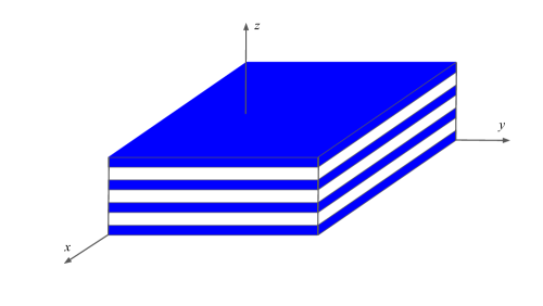
Figure 2: An illustration of a uniaxial nanolayered metamaterial

Now, for the sake of completeness, we shall find a matrix equation to find the temperature profile of a layered uniaxial medium (Fig. 2) which has been made by repeated copies of a bilayer reciprocal medium for which we can define the effective transverse and axial phononic thermal conductivities, based on the effective medium theory, as $\overline{\overline{\alpha}}_{c}=\overline{\overline{\alpha}}_{c_{t}}+\overline{\overline{\alpha}}_{c_{z}}$. For simplicity and without losing the generality, we assume $g_{c}=0$ and $dL_{p}/dt=0$ in Eq. (5). Working in the cylindrical coordinate system, it is also a reasonable assumption for paraxial media that there is no azimuthal variation in temperature profile. Now, by rewriting Eq. (5) in the cylindrical coordinate system we have

$$\bar{\alpha}_{c_{v}}\dot{T}(\rho,z,t)+\alpha_{c_{t}}\left(\rho^{-1}\partial_{\rho}+\partial^{2}_{\rho}\right)T(\rho,z,t)+\alpha_{c_{z}}\partial^{2}_{z}T(\rho,z,t)=\mathcal{S}_{hp}(\rho,z,t),$$ (92)

where $\mathcal{S}_{hp}=(h_{EM}-p_{rad})_{{}_{\omega_{0}}}$ and $\bar{\alpha}_{c_{v}}$ is the volumetric averaged value of $\varrho_{m}c_{v}$ for the medium. In the above equation, within the framework of effective medium theory [69], $\alpha_{c_{z}}$ and $\alpha_{c_{t}}$ denote

$$\alpha_{c_{z}}={\alpha^{m}_{c}\alpha^{h}_{c}\over\alpha^{m}_{c}(1-f)+\alpha^{h}_{c}f},\qquad\alpha_{c_{t}}=\alpha^{m}_{c}f+\alpha^{h}_{c}(1-f),$$ (93)

with $\alpha^{m(h)}_{c}$ and $f$ as the phononic thermal conductivity of the embedded medium (or host) and the volume fraction of the medium, respectively. Recalling Eqs. (54) and (56), the right-hand side of Eq. (92), $\mathcal{S}_{hp}(\vec{r},t)$ is replaced by $\mathcal{S}^{c}_{hp}$ which is defined as $\mathcal{S}^{c}_{hp}=(h^{a,c}_{EM}-p^{c}_{rad})_{{}_{\omega_{0}}}$ (cf. Eqs. (4.1) and (4.2)).

In order to obtain the profile of temperature, the non-homogeneous integro-differential equation, Eq. (92), needs to be solved. We aim to present a closed-form relation for solution of Eq. (92). For this purpose, we consider the stationary state heat transfer in the medium. By setting $\dot{T}=0$ in Eqs. (4.1) and (4.2), Eq. (92), in the cylindrical coordinates, reads

$$\alpha_{c_{t}}\nabla_{\rho}^{2}T(\rho,z)+\alpha_{c_{z}}\partial^{2}_{z}T(\rho,z)=\mathcal{S}^{c,st}_{hp}(\rho,z),$$ (94)

where the right-hand side of the equation above is given by

$$\mathcal{S}^{c,st}_{hp}=(h^{a,c,st}_{EM}-p^{c,st}_{rad})_{{}_{\omega_{0}}},$$ (95)

In Eq. (95), the superscript $st$ emphasizes that we considered steady state conditions and $h^{a,c,st}_{EM}$ and $p^{c,st}_{rad}$ call

$$h^{a,c,st}_{EM}= k_{B}\sum_{\alpha,\beta,\gamma}F^{a,c,st}_{\alpha,\beta,\gamma}\int_{z_{i}}^{z_{f}}dz^{\prime}\int_{0}^{\infty}\rho^{\prime}d\rho^{\prime}|I^{\gamma}_{\alpha\beta}(\rho^{\prime},|z-z^{\prime}|)|^{2}T(\rho^{\prime},z^{\prime}),$$

$$p^{c,st}_{EM}= k_{B}\sum_{\alpha,\gamma}Q^{c,st}_{\alpha,\gamma}T(\rho,z),$$ (96)

with $F^{a,c,st}_{\alpha,\beta,\gamma}$ and $Q^{c,st}_{\alpha,\gamma}$ expressed as follows

$$F^{a,c,st}_{\alpha,\beta,\gamma}={\triangle\omega\over\pi^{4}} \bigg{[}a^{\alpha}_{0_{t}}a^{\beta}_{0_{t}}(|C^{\,a,\gamma}_{\alpha\beta}|^{2}+\triangle\omega^{2}|D^{\,a,\gamma}_{\alpha\beta}|^{2}/12)-{\triangle\omega^{2}\over 4}a^{\alpha}_{0_{t}}a^{\beta}_{1_{t}}\mathfrak{R}\!\left(C^{\,a,\gamma}_{\alpha\beta}\,D^{\,a,\gamma\,*}_{\alpha\beta}\right)\bigg{]}_{{}_{\omega_{0}}},$$

$$Q^{c,st}_{e[m],\gamma}=[-]{\triangle\omega\over\pi^{4}}\mathfrak{R}\!\sum_{\gamma,j}\left[\Pi^{\gamma[*]}_{e[m],j}\,a^{e[m]}_{0j}+{\triangle\omega^{2}\over 12}\partial_{\omega}(\Pi^{\gamma[*]}_{e[m],j})a^{e[m]}_{1_{j}}\right]_{{}_{\omega_{0}}}.$$ (97)

In order to solve Eq. (94), let us rewrite it as follows

$$\alpha_{c_{t}}\left(\rho^{-1}\partial_{\rho}+\partial^{2}_{\rho}\right)T(\rho,z)+\alpha_{c_{z}}\partial^{2}_{z}T(\rho,z)+\alpha_{Q}T(\rho,z)=\mathcal{T}^{a,c,st},$$

$$\mathcal{T}^{a,c,st}=k_{B}\sum_{\alpha,\beta,\gamma}F^{a,c,st}_{\alpha,\beta,\gamma}\int_{z_{i}}^{z_{f}}dz^{\prime}\int_{0}^{\infty}\rho^{\prime}d\rho^{\prime}|I^{\gamma}_{\alpha\beta}(\rho^{\prime},|z-z^{\prime}|)|^{2}T(\rho^{\prime},z^{\prime}),$$ (98)

where $\alpha_{Q}=k_{B}\sum_{\alpha,\gamma}Q^{c,st}_{\alpha,\gamma}$. By setting a Gaussian transverse profile, we consider the following expansion of $T(\rho,z)$ in the cylindrical coordinates

$$T(\rho,z)=e^{-\alpha_{\sigma}\rho^{2}}\sum_{n=0}^{\infty}\rho^{n}\,T_{n}(z),\qquad\alpha_{\sigma}=1/(2\sigma_{\rho})\,.$$ (99)

Thus, to find the temperature profile, we need to obtain $T_{n}(z)$ for each value of the order $n=0,1,2,...$ at each point $z\in(z_{i},z_{f})$, i.e. between the input and output interfaces of a nanolayered metamaterial, respectively. In order to obtain $T_{n}(z)$, first, we ignore the source term in Eq. (5), $\mathcal{T}^{a,c,st}$, and thus we obtain the following differential equation:

$$\alpha_{c_{t}}\left(\rho^{-1}\partial_{\rho}+\partial^{2}_{\rho}\right)T(\rho,z)+\alpha_{c_{z}}\partial^{2}_{z}T(\rho,z)=0.$$ (100)

Next, we recall the Gaussian transverse temperature profile and the solution presented by Eq. (99), and, by employing an analogy with the method of separation of variables and using the Frobenius method within the yielded differential equation, we look for a second-order differential equation for $T_{n}(z)$. Finally, we include the source term and find an integro-differential equation that has to be solved at each value of $n$.

Before implementing this strategy, let us take a closer look at $f(\rho,n)=\rho^{n}e^{-\alpha_{\sigma}\rho^{2}}$. In Fig. 3, we plot $f_{\mathcal{N}}(\rho,n)$ versus $\rho$ for $n=0,1,\ldots 5$, where the index $\mathcal{N}$ denotes that $f(\rho,n)$ has been normalized by its maximum value at each $n$. In this numerical example, we set $\sigma_{\rho}=0.5$. As can be seen, the peak of $f_{\mathcal{N}}(\rho,n)$ shifts forward as $n$ increases and the peak positions become closer to each other at higher $n$’s.

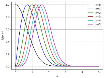
Figure 3: Variation of $f_{\mathcal{N}}(\rho,n)$ versus $\rho$ for $n=0-5$ and $\alpha=1$ (see text).

In order to find $T_{n}(z)$, we use the Frobenius method. After some algebra, we obtain

$$\alpha_{c_{t}}\sum_{n=0}^{\infty}T_{n}(z)\left(\rho^{-1}\partial_{\rho}+\partial^{2}_{\rho}\right)\rho^{n+k}e^{-\alpha_{\sigma}\rho^{2}}+\alpha_{c_{z}}\sum_{n=0}^{\infty}T^{\prime\prime}_{n}(z)\rho^{n+k}e^{-\alpha_{\sigma}\rho^{2}}=0,$$ (101)

where $T^{\prime\prime}_{n}(z)$ is the second-order derivative of $T_{n}(z)$ with respect to $z$. After calculating the derivatives in Eq. (101), solving the yielded equation for $k$, which results in $k=0$, and using Eq. (99) within the source term $\mathcal{T}^{a,c,st}$ given by Eq. (5), we obtain the following equation:

$$T^{\prime\prime}_{n}(z)+[\lambda_{Q}-(n+1)\lambda_{0}] \,T_{n}(z)+(n+2)^{2}\lambda_{z}T_{n+2}(z)+\lambda_{\sigma}\theta(n-2)\,T_{n-2}(z)=\mathcal{T}^{a,c,st},$$

$$\mathcal{T}^{a,c,st}=\lambda_{\rho}\int_{z_{i}}^{z_{f}}M_{n}(z,z^{\prime})\,T_{n}(z^{\prime})dz^{\prime},\quad n=0,1,...,$$ (102)

where $\theta(\cdot)$ is the Heaviside function and $M_{n}(z,z^{\prime})$ is given by

$$M_{n}(|z-z^{\prime}|)=\sum_{\alpha,\beta,\gamma}F^{a,c,st}_{\alpha,\beta,\gamma}\int_{0}^{\infty}d\rho^{\prime}\rho^{\prime n+1}e^{-\alpha_{\sigma}\rho^{\prime 2}}|I^{\gamma}_{\alpha\beta}(\rho^{\prime},|z-z^{\prime}|)|^{2}.$$ (103)

The parameters in Eq. (5) read

$$\lambda_{\rho}=k_{B}e^{-\alpha_{\sigma}\rho^{2}}/\alpha_{c_{z}},$$

$$\lambda_{Q}=\alpha_{Q}/\alpha_{c_{z}},$$

$$\lambda_{z}=\alpha_{c_{t}}/\alpha_{c_{z}},$$

$$\lambda_{0}=4\alpha_{\sigma}\lambda_{z},$$

$$\lambda_{\sigma}=\alpha_{\sigma}\lambda_{0}.$$ (104)

With the closed-form expression of $|I^{\gamma}_{\alpha\beta}(\rho^{\prime},|z-z^{\prime}|)|^{2}$ (see Appendix B, Eq. (Appendix B: Calculation of $|I\,^{\gamma}(\vec{R})|^{2}$) ), one can integrate over $\rho^{\prime}$ and obtain the closed-form expression of $M_{n}(|z-z^{\prime}|)$ (Appendix D).

In order to solve Eq. (5), which is the second-order Fredholm integro-differential equation, we consider the Dirichlet boundary conditions, in which $T_{n}(z_{i})=T^{n}_{0}$ and $T_{n}(z_{f})=T^{n}_{N}$ are known. To proceed with the solution, we use the quadrature-difference method that exploits a combination of Composite Simpson’s 1/3 rule and the second-order finite-difference approach.

According to this method, the left-hand side of Eq. (5) can be rewritten in terms of forward, central, and backward differences to calculate the second-order derivative of $T_{n}(z)$ with respect to $z$ (up to $O(h^{4})$ with $h=(z_{i}-z_{f})/N$ as the step size) as follows

Forward difference

$$T^{\prime\prime}_{n}(z_{1})={1\over 12h^{2}}\left[\iota_{1}T_{n}(z_{1})+\iota_{2}T_{n}(z_{2})+\iota_{3}T_{n}(z_{3})+\iota_{4}T_{n}(z_{4})+\iota_{5}T_{n}(z_{5})\right],$$

Central difference

$$T^{\prime\prime}_{n}(z_{m})={1\over 12h^{2}}\left[\iota_{6}T_{n}(z_{m-2})+\iota_{7}T_{n}(z_{m-1})+\iota_{8}T_{n}(z_{m})+\iota_{7}T_{n}(z_{m+1})+\iota_{6}T_{n}(z_{m+2})\right],$$

$$\qquad\qquad\qquad\qquad\qquad\qquad 1<m<N-1,$$

Backward difference

$$T^{\prime\prime}_{n}(z_{N-1})={1\over 12h^{2}}\left[\iota_{1}T_{n}(z_{N-1})+\iota_{2}T_{n}(z_{N-2})+\iota_{3}T_{n}(z_{N-3})+\iota_{4}T_{n}(z_{N-4})+\iota_{5}T_{n}(z_{N-5})\right],$$

where $\iota$’s coefficients are as follows

$$\iota_{1}=35,\qquad\iota_{2}=-104,\qquad\iota_{3}=114,\qquad\iota_{4}=-56,$$

$$\quad\iota_{5}=11,\qquad\iota_{6}=-1,\qquad\iota_{7}=16,\qquad\iota_{8}=-30.$$ (106)

Regarding the Composite Simpson’s 1/3 rule, the right-hand side of Eq. (5) can be written as follows

$$\lambda_{\rho}\int_{z_{i}}^{z_{f}}M_{n}(z,z^{\prime}) \,T_{n}(z^{\prime})dz^{\prime}=\lambda_{\rho}\,h/3\times\big{[}M_{n}(z_{m},z_{i})\,T_{n}(z_{i})+M_{n}(z_{m},z_{N})\,T_{n}(z_{N})$$

$$+\sum_{l=1}^{N-1}\left[4M_{n}(z_{m},z_{2l-1})T_{n}(z_{2l-1})+2M_{n}(z_{m},z_{2l})T_{n}(z_{2l})\right]\big{]},$$ (107)

with $1<m<N-1$. To find a matrix equation for computing each $T_{n}(z_{m})$, without any loss of generality, we consider the first five terms of the forward and backward differences in Eq. (5). Now, by denoting $T_{n}(z_{m})$ as $T^{n}_{m}$ and $M_{n}(z_{m},z_{l})$ as $M^{n}_{ml}$ and recalling Eqs.(5) and (5), Eq. (5) reads:

$$\mbox{if}\;m=1\;\mbox{or}\;N-1:$$ (108)

$${1\over 12h^{2}}\left[\iota_{1}T^{n}_{m}+\iota_{2}T^{n}_{m\pm 1}+\iota_{3}T^{n}_{m\pm 2}+\iota_{4}T^{n}_{m\pm 3}+\iota_{5}T^{n}_{m\pm 4}\right]+$$

$$(\lambda_{Q}-(n+1)\lambda_{0})T^{n}_{m}+(n+2)^{2}\lambda_{z}\,T^{n+2}_{m}+\lambda_{\sigma}\theta(n-2)\,T^{n-2}_{m}=\mathcal{M}^{n}_{m},$$

$$\mbox{and if}\;2\leq m\leq N-2:$$

$${1\over 12h^{2}}\left[\iota_{6}T^{n}_{m-2}+\iota_{7}T^{n}_{m-1}+\iota_{8}T^{n}_{m}+\iota_{6}T^{n}_{m+1}+\iota_{6}T^{n}_{m+2}\right]+$$

$$(\lambda_{Q}-(n+1)\lambda_{0})T^{n}_{m}+(n+2)^{2}\lambda_{z}T^{n+2}_{m}+\lambda_{\sigma}\theta(n-2)\,T^{n-2}_{m}=\mathcal{M}^{n}_{m},$$

where

$$\mathcal{M}^{n}_{m}={\lambda_{\rho}\,h\over 3}\left[M^{n}_{m0}\,T^{n}_{0}+M^{n}_{mN}\,T^{n}_{N}\sum_{l=1}^{N-1}(4M^{n}_{m,2l-1}\,T^{n}_{2l-1}+2M^{n}_{m,2l}\,T^{n}_{2l})\right].$$ (109)

Above, $\pm$ within terms with indices of $m\pm 1$, etc, where $m=1$ or $(N-1)$, shows the forward or backward difference, respectively. Now, by manipulating Eq. (108), one can write a matrix equation as follows:

$$\overline{\overline{\bf{O}}}\,^{n}\cdot\vec{\bf{T}}^{n}+P^{n+2}\vec{\bf{T}}^{n+2}+Q^{n-2}\vec{\bf{T}}^{n-2}=\vec{\bf{U}}^{n},\qquad n=0,1,2,...,$$

$$P^{n+2}=12(n+2)^{2}\lambda_{z}h^{2},\qquad Q^{n-2}=12\theta(n-2)\lambda_{z}h^{2},$$ (110)

where $\vec{\bf{T}}^{n}$ and $\vec{\bf{U}}^{n}$ are $(N-1)$-dimensional column vectors, whose elements are given by $T^{n}_{1},T^{n}_{2},...,T^{n}_{N-2},T^{n}_{N-1}$ and $U^{n}_{i}=4\lambda_{\rho}[(M^{n}_{i0}+\delta_{i0})T^{n}_{0}+(M^{n}_{iN}+\delta_{i,N-2})T^{n}_{N}]h^{3}$, respectively, with $\delta_{ij}$ being the Kronecker delta, $h$ being the step size, and $N$ being the total number of steps. The $(N-1)\times(N-1)$ matrix $\overline{\overline{\bf{O}}}\,^{n}$ has the following form

$$\overline{\overline{\bf{O}}}\,^{n}=\begin{bmatrix}\vec{\bf{a}}^{\,n}_{1}&\vec{\bf{b}}^{\,n}_{2}&\vec{\bf{a}}^{\,n}_{3}&\vec{\bf{b}}^{\,n}_{4}&\vec{\bf{a}}^{\,n}_{5}&\vec{\bf{b}}^{\,n}_{6}&...&\vec{\bf{b}}^{\,n}_{N-2}&\vec{\bf{a}}^{\,n}_{N-1}\\ \end{bmatrix}+\overline{\overline{\textbf{$\iota$}}}$$ (111)

where $\vec{\bf{a}}^{\,n}_{j}$ and $\vec{\bf{b}}^{\,n}_{j}$ are the column vectors with the following elements:

$$a^{n}_{ij}=-16\lambda_{\rho}M^{n}_{ij}h^{3},\qquad b^{n}_{ij}=-8\lambda_{\rho}M^{n}_{ij}h^{3},$$ (112)

and $\overline{\overline{\textbf{$\iota$}}}$, an $N-1$ $\times$ $N-1$ matrix, is given by

$$\overline{\overline{\textbf{$\iota$}}}=\begin{bmatrix}a_{0}&\iota_{2}&\iota_{3}&\iota_{4}&\iota_{5}&0&...&0&0\\ \iota_{7}&b_{0}&\iota_{7}&\iota_{6}&0&0&...&0&0\\ \iota_{6}&\iota_{7}&b_{0}&\iota_{7}&\iota_{6}&0&...&0&0\\ 0&\iota_{6}&\iota_{7}&b_{0}&\iota_{7}&\iota_{6}&...&0&0\\ 0&0&\iota_{6}&\iota_{7}&b_{0}&\iota_{7}&...&0&0\\ .&.&.&.&.&.&...&.&.\\ .&.&.&.&.&.&...&.&.\\ .&.&.&.&.&.&...&.&.\\ 0&0&...&b_{0}&\iota_{7}&\iota_{6}&...&0&0\\ 0&0&...&\iota_{7}&b_{0}&\iota_{7}&...&\iota_{6}&0\\ 0&0&...&\iota_{6}&\iota_{7}&b_{0}&...&\iota_{7}&\iota_{6}\\ 0&0&...&0&\iota_{6}&\iota_{7}&...&b_{0}&\iota_{7}\\ 0&0&...&\iota_{5}&\iota_{4}&\iota_{3}&...&\iota_{2}&a_{0}\\ \end{bmatrix},$$ (113)

where $a_{0}=\iota_{1}+12(\lambda_{Q}-(n+1)\lambda_{0})h^{2}$ and $b_{0}=\iota_{8}+12(\lambda_{Q}-(n+1)\lambda_{0})h^{2}$.

Thus, one can solve the second-order differential equation for the each order of temperature, $T^{n}(z)$, and then use Eq. (99) to obtain and expression for the temperature profile. With the temperature profile at hand, one can find the radiative heat flux, Eq. (4.3), and, in turn, the radiative heat conductivity as well.

6 Conclusion

By employing the novel concept of EDGF, rather than the standard DGF technique, we have developed a self-consistent theoretical method for modeling the DHT in DDANM, such as MMs. To model the propagation of thermally-agitated fluctuations of electromagnetic fields through DDANM, which involves modeling of dynamic heat storage and release due to both photonic and phononic processes, we assumed that the photonic radiative heat transfer mechanisms in DDANM are complemented with dynamic phononic mechanisms of heat storage and conduction, taking into account the effects of local heating, heat storage, release, and material phase transitions. Furthermore, we have developed a theoretical framework for studying the propagation of quasi-monochromatic signals through dispersive and dissipative media. By representing the time-dependent EM fields associated with such processes as products of the slowly varying amplitude and the quickly oscillating carrier, we have formulated a system of equations for the SVAs of the electromagnetic fields in such media.

We solved the Maxwell macroscopic equations using this method and employed the Poynting and fluctuating-dissipative theorems for the propagation of FEFs. We obtained a closed form expression for the coupling term of the photonic-phononic mechanism by using macroscopic electro- and thermodynamics. Then, we applied the yielded closed-form relations for modeling of the paraxial radiative heat transfer in DDAN uniaxial MMs. By considering a Gaussian form for the transverse profile of temperature, we obtained a second-order Fredholm integro-differential equation for heat diffusion in the steady-state case, which can be used to model the paraxial heat transfer in such media. Using the quadrature-difference method, we solved the Fredholm equation and found the temperature profile. With this profile, one can calculate the radiative heat flux and, in turn, the radiative heat conductivity. The results of this research may find applications in the areas of science and technology related to nanoantennas, nanolithography, thermophotovoltaics, energy harvesting, RHT cooling, and microfluidic/nanofluidic thermal management.

With minimal adaptations, the developed framework can be used to model coupled electromagnetic wave and heat propagation through a material whose parameters may depend on the local temperature, which is affected by the passing electromagnetic radiation. We plan to present such an extension of this method in a future work.

Appendix A: Extracting PEDGF

To give an extract of the the EDGF formalism, we consider uniaxial media with the material dyadics of the form

$$\overline{\overline{\zeta}}\,^{\alpha}=\zeta_{t}^{\alpha}\overline{\overline{I}}_{t}+\zeta_{z}^{\alpha}\overline{\overline{I}}_{z},\qquad\alpha=e\ \mbox{or}\ m,$$ (114)

with $\overline{\overline{I}}_{t}=\hat{x}\hat{x}+\hat{y}\hat{y}$ and $\overline{\overline{I}}_{z}=\hat{z}\hat{z}$ as the identity dyadics in two orthogonal directions: the tangential and axial, where we can decompose the propagation wave vector as $\vec{k}\times\overline{\overline{I}}=(\vec{k}_{t}+\vec{k}_{z})\times(\overline{\overline{I}}_{t}+\overline{\overline{I}}_{z})$. From the EDGF formalism of Ref. [65], the envelope dyadic Green’s function in the cylindrical coordinates, as sum of two orthogonal polarizations, TE($p$) and TM($s$), is given by

$$\overline{\overline{\bf{G}}}(k_{t},\vec{\varrho},\pm|Z|;\triangle\omega,\tau)={\triangle\omega\over(2\pi)^{3}}\sum_{\gamma=p,s} \bigg{\{}\int d\vec{k}_{t}e^{i(\vec{k}_{t}\cdot\vec{\varrho}+\kappa^{\gamma}_{0}|Z|)}$$

$$\times\left[j_{0}(\tau_{g}^{\gamma}\triangle\omega/2)\,\overline{\overline{\bf{C}}}-i{\triangle\omega\over 2}j_{1}(\tau_{g}^{\gamma}\triangle\omega/2)\,\overline{\overline{\bf{D}}}\right]\bigg{\}}_{\omega_{0}},$$ (115)

where $\vec{\varrho}=\vec{\rho}-\vec{\rho}^{\,\prime}$ and $|Z|=|z-z^{\,\prime}|$. In the above equation, we have expanded $\vec{r}$ and $\vec{r}^{\,\prime}$ as $\vec{r}=(\vec{\rho},\vec{z}\,)$ and $\vec{r}^{\,\prime}=(\vec{\rho}^{\,\prime},\vec{z}^{\,\prime})$, respectively. The notations $j_{0}(\cdot)$ and $j_{1}(\cdot)$ represent the zeroth- and first-order spherical Bessel functions, and $\tau_{g}^{\gamma}=\tau-Z/V^{\gamma}_{g}$ with $V^{\gamma}_{g}$ as the group velocity of FEFSVA. The propagation factor $\kappa^{\gamma}_{0}$ and the group velocity read

$$\kappa^{p[s]}_{0}=\sqrt{a^{e}_{t}a^{m}_{t}-a^{e[m]}_{t}k_{t}^{2}/a^{e[m]}_{z}},\quad\mathfrak{I}(\kappa_{p[s]})>0,$$ (116)

$$V^{p[s]}_{g}={2\kappa^{\gamma}_{0}\over(a^{e}_{t}b^{m}_{t}+a^{m}_{t}b^{e}_{t})-(b^{e[m]}_{t}a^{e[m]}_{z}-a^{e[m]}_{t}b^{e[m]}_{z})k_{t}^{2}/a^{e[m]^{2}}_{z}},\quad$$ (117)

with

$$a^{e}_{i}=\omega\varepsilon_{i},\qquad b^{e}_{i}=\partial_{\omega}(\omega\varepsilon_{i}),\qquad\mbox{(TM)},$$ (118)

$$a^{m}_{i}=\omega\mu_{i},\qquad b^{m}_{i}=\partial_{\omega}(\omega\mu_{i}),\qquad\mbox{(TE)},$$ (119)

with the index $i$ denotes $t$ and $z$. Reader can find the components of $\overline{\overline{\bf{C}}}$ and $\overline{\overline{\bf{D}}}$ in Ref. [65].

Now, for the paraxial propagation case, the propagation factor and the group velocity are given in Ref. [65]:

$$\kappa^{p[s]}_{0}=\kappa_{a}\sqrt{1-{a^{e[m]}_{t}k_{t}^{2}\over a^{e[m]}_{z}\kappa_{a}^{2}}},\qquad V_{g}^{a}={2\kappa_{a}\over(a_{t}^{e}b^{m}_{t}+a^{m}_{t}b^{e}_{t})},\qquad\kappa_{a}=\sqrt{a^{e}_{t}a^{m}_{t}}.$$ (120)

As can be seen in Eq. (120), $V^{a}_{g}$ is no longer dependent on the polarization of the propagation and also $k_{t}$. Thus, we can find $\tau^{\gamma}_{g,paraxial}\equiv\tau_{a}=\tau-|Z|/V^{a}_{g}$ is also independent of polarization and $k_{t}$. When $\left|a^{e[m]}_{z}k_{t}^{2}\right|\ll\left|a^{e[m]}_{z}\kappa_{a}^{2}\right|$, we can expand $\kappa_{0}^{p[s]}$ as follows

$$\kappa^{p[s]}_{0}\approx\kappa_{a}-{1\over 2}{a^{e[m]}_{t}k_{t}^{2}\over a^{e[m]}_{z}\kappa_{a}}.$$ (121)

Regarding independence of $V^{a}_{g}$ and $\tau_{a}$ on $k_{t}$ and polarization, and setting $k_{t}\approx 0$ in $\overline{\overline{\bf{C}}}$ and $\overline{\overline{\bf{D}}}$ [65], the PEDGF, $\overline{\overline{\bf{G}}}\,^{a}(k_{t},\vec{\varrho},\pm|Z|;\triangle\omega,\tau)$, can be reduced to

$$\overline{\overline{\bf{G}}}\,^{a}={\triangle\omega\over(2\pi)^{3}}\bigg{\{} e^{i\kappa_{a}|Z|}\sum_{\gamma=p,s}\int d\vec{k}_{t}e^{i(\vec{k}_{t}\cdot\vec{\varrho}-\chi^{\gamma}_{a}k_{t}^{2})}$$ (122)

$$\times\left[j_{0}(\tau_{a}\triangle\omega/2)\,\overline{\overline{\bf{C}}}\,^{\gamma}_{a}-i{\triangle\omega\over 2}j_{1}(\tau_{a}\triangle\omega/2)\,\overline{\overline{\bf{D}}}\,^{\gamma}_{a}\right]\bigg{\}}_{\omega_{0}},$$

where $\chi^{\gamma}_{a}=\xi^{\gamma}/2\kappa_{a}$ with $\xi^{p[s]}={a^{e[m]}_{t}\over a^{e[m]}_{z}}|Z|$ and $\overline{\overline{\bf{C}}}_{a}$ and $\overline{\overline{\bf{D}}}_{a}$ are given by:

$$\overline{\overline{\bf{C}}}\,^{\gamma}_{a}=\begin{bmatrix}\overline{\overline{C}}\,^{tt,\gamma}_{a}&&\overline{\overline{0}}\\ \overline{\overline{0}}&&\overline{\overline{0}}\end{bmatrix},\qquad\overline{\overline{\bf{D}}}\,^{\gamma}_{a}=\begin{bmatrix}\overline{\overline{D}}\,^{tt,\gamma}_{a}&&0\\ \overline{\overline{0}}&&\overline{\overline{0}}\end{bmatrix}.$$ (123)

Removing superscript $tt$ from the different matrix elements of $\overline{\overline{C}}\,^{tt}_{a}$ and $\overline{\overline{D}}\,^{\,tt}_{a}$, the dyadic matrix forms, denoted here by $\overline{\overline{M}}_{a}$ expressed as

$$\overline{\overline{M}}_{a}\equiv\begin{bmatrix}M^{a,p}_{ee}\,\overline{\overline{e}}\,^{p}_{ee}&&M^{a,p}_{em}\,\overline{\overline{e}}\,^{p}_{em}\\ M^{a,p}_{me}\,\overline{\overline{e}}\,^{p}_{me}&&M^{a,p}_{me}\,\overline{\overline{e}}\,^{p}_{mm}\end{bmatrix}\,+\begin{bmatrix}M^{a,s}_{ee}\,\overline{\overline{e}}\,^{s}_{ee}&&M^{a,s}_{em}\,\overline{\overline{e}}\,^{s}_{em}\\ M^{a,s}_{em}\,\overline{\overline{e}}\,^{s}_{em}&&M^{a,s}_{mm}\,\overline{\overline{e}}\,^{s}_{mm}\end{bmatrix},$$ (124)

where the different non-zero elements of $M^{a,\gamma}_{\alpha\beta}$, with $M=C,D$, are calculated by setting $k_{t}\approx 0$ for different elements of $\overline{\overline{\bf{C}}}$ and $\overline{\overline{\bf{D}}}$ [65], we obtain

$$C^{a,\gamma}_{ee[mm]}=-{a^{m[e]}_{t}\over 2\kappa_{a}},\qquad C^{a,\,s[p]}_{em[me]}=[-]{n_{z}\over 2},$$ (125)

$$D^{a,\gamma}_{ee[mm]}=-[+]{a^{m[e]}_{t}\over 4\kappa_{a}}\left({b_{t}^{m}\over{a_{t}^{m}}}-{b_{t}^{e}\over{a_{t}^{e}}}\right),$$ (126)

with $n_{z}=+1\,or-1$, depending on the sign of $Z$, that is, $Z>0\,or\,Z<0$. In Eq. (124), $\overline{\overline{e}}\,^{\gamma}_{\alpha\beta}$ are given by [65]

$$\overline{\overline{e}}\,^{p[s]}_{ee[mm]}=\hat{t}\hat{t},\qquad\overline{\overline{e}}\,^{p[s]}_{mm[ee]}=\hat{s}\hat{s},\qquad\overline{\overline{e}}\,^{p[s]}_{em}=\hat{t}\hat{s},\qquad\overline{\overline{e}}\,^{p[s]}_{me}=\hat{s}\hat{t},$$ (127)

where $\hat{t}=\vec{k_{t}}/k_{t}$ and $\hat{s}=\hat{z}\times\hat{t}$. Now, remembering that the PEDGF block matrix has only the transverse-transverse block element, the general form of PDGF elements is given by

$$\overline{\overline{G}}\,^{a,\gamma}_{\alpha\beta}=[\triangle\omega/(2\pi)^{3}]\, \left[C\,^{a,\gamma}_{\alpha\beta}j_{0}(\tau_{a}\triangle\omega/2)-i(\triangle\omega/2)D\,^{a,\gamma}_{\alpha\beta}j_{1}(\tau_{a}\triangle\omega/2)\right]\,\overline{\overline{I}}\,^{\gamma}_{\alpha\beta}(\vec{\varrho},|Z|),$$

$$\overline{\overline{I}}\,^{\gamma}_{\alpha\beta}(\vec{\varrho},|Z|)=e^{i\kappa_{a}|Z|}\int d\vec{k}_{t}e^{i[\vec{k}_{t}\cdot\vec{\varrho}-\chi^{\gamma}_{a}k_{t}^{2}]}\,\overline{\overline{e}}\,^{\gamma}_{\alpha\beta}.$$ (128)

Appendix B: Calculation of $|I\,^{\gamma}(\vec{R})|^{2}$

In order to calculate the integral over $\vec{k}_{t}$ in $\overline{\overline{I}}^{\gamma}_{\alpha\beta}(\vec{\varrho},|Z|)$, we can rewrite Eq. (Appendix A: Extracting PEDGF) by setting $\nabla_{t}=i\vec{k_{t}}$ where $\nabla_{t}$ is the gradient operator in the transverse plane, which, in cylindrical coordinates, reads $\nabla_{t}=\partial_{\varrho}\,\hat{\varrho}+\partial_{\phi}\,\hat{\phi}/\varrho$. Thus, Eq. (127) reads:

$$\overline{\overline{e}}\,^{p[s]}_{ee[mm]}=-\nabla_{t}\nabla_{t}/k_{t}^{2},\qquad\overline{\overline{e}}\,^{p[s]}_{mm[ee]}=-\hat{z}\times\nabla_{t}\hat{z}\times\nabla_{t}/k_{t}^{2},$$

$$\overline{\overline{e}}\,^{p[s]}_{em}=-\nabla_{t}\hat{z}\times\nabla_{t}/k_{t}^{2},\qquad\overline{\overline{e}}\,^{p[s]}_{me}=-\hat{z}\times\nabla_{t}\nabla_{t}/k_{t}^{2}.$$ (129)

As can be seen in above, all dyadic operators $\overline{\overline{e}}\,^{\gamma}_{\alpha\beta}$ contain $k_{t}^{2}$. So, by keeping $k_{t}^{2}$ in the integral over $\vec{k_{t}}$ in $\overline{\overline{I}}\,^{\gamma}_{\alpha\beta}(\vec{\varrho},|Z|)$ and taking the rest out of the integral, we need to solve the following simple integral

$$I\,^{\gamma}(\vec{\varrho}\,)=\int e^{i\vec{k}_{t}\cdot\vec{\varrho}}\,\left[e^{-i\chi^{\gamma}_{a}k_{t}^{2}}/k_{t}^{2}\right]d\vec{k}_{t},$$ (130)

where we have not included the factor of $e^{i\kappa_{a}|Z|}$. In above, the bracketed expression can be written in an integral form as $\int_{-\infty}^{-i\chi^{\gamma}_{a}}d\eta e^{\eta k_{t}^{2}}$. By setting $\eta\rightarrow-i\eta$, we rewrite Eq. (130) as follows:

$$I\,^{\gamma}(\vec{\varrho}\,)=-i\int_{-i\infty}^{\chi^{\gamma}_{a}}d\eta\left[\int e^{i[\vec{k}_{t}\cdot\vec{\varrho}-i\eta k_{t}^{2}]}d\vec{k}_{t}\right].$$ (131)

By expanding $\vec{\varrho}=\vec{X}+\vec{Y}$ and decomposing the integral over $\vec{k}_{t}$ into two integrals over $k_{x}$ and $k_{y}$, we have

$$I\,^{\gamma}(X,Y)=-i\int_{-i\infty}^{\chi^{\gamma}_{a}}d\eta\left[\int_{-\infty}^{\infty}dk_{x}\,e^{i(k_{x}\,X-\eta k_{x}^{2})}\right]\left[\int_{-\infty}^{\infty}dk_{y}\,e^{i(k_{y}\,Y-\eta k_{y}^{2})}\right].$$ (132)

Since two integrals in brackets are the same except for the dummy variables $k_{x}$ and $k_{y}$, we go on by considering one of them and have

$$\int_{-\infty}^{\infty}dk_{x}\,e^{i(k_{x}\,X-\eta k_{x}^{2})}=e^{iX^{2}/4\eta}\int_{-\infty}^{\infty}dK_{x}\,e^{-i\eta K_{x}^{2}},\qquad K_{x}=k_{x}-X/2\eta.$$ (133)

Substituting this result into Eq. (131), recalling $\int_{0}^{\infty}e^{-iax^{2}}xdx=1/(2ia)$ with $a$ as a complex number, after some manipulation, we have

$$I\,^{\gamma}(\varrho)=-\pi\int_{-i\infty}^{\chi^{\gamma}_{a}}d\eta e^{i\varrho^{2}/4\eta}/\eta.$$ (134)

Now, we are ready to include the dyadic parts of $\overline{\overline{I}}\,^{\gamma}_{\alpha\beta}(\vec{\varrho})$. Noticing that $\nabla_{t}$ and $\hat{z}\times\nabla_{t}$ depend on $\hat{\rho}$ and $\hat{\phi}$ and the integrand in Eq. (134) does not depend on the azimuthal angle $\phi$, for all components of $\overline{\overline{I}}\,^{\gamma}_{\alpha\beta}(\vec{\varrho})$ except $\overline{\overline{I}}\,^{\gamma}_{me}(\vec{\varrho})$ we arrive at the following integral:

$$\overline{\overline{I}}\,^{\gamma}_{\alpha\beta}(\vec{\varrho}\,)=-\pi\overline{\overline{u}}\,^{\gamma}_{\alpha\beta}\partial_{\varrho}\partial_{\varrho}\int_{-i\infty}^{\chi^{\gamma}_{a}}d\eta e^{i\varrho^{2}/4\eta}/\eta.$$ (135)

where the dyadics $\overline{\overline{u}}\,^{\gamma}_{\alpha\beta}$ are as follows:

$$\overline{\overline{u}}\,^{p[s]}_{ee[mm]}=-\hat{\rho}\hat{\rho},\qquad\overline{\overline{u}}\,^{p[s]}_{mm[ee]}=-\hat{\phi}\hat{\phi},\qquad\overline{\overline{u}}\,^{p[s]}_{em}=-\hat{\rho}\hat{\phi}.$$ (136)

For the case of $\overline{\overline{I}}\,^{\gamma}_{me}(\vec{\varrho}\,)$, we have

$$\overline{\overline{I}}\,^{\gamma}_{me}(\vec{\varrho}\,)=-\pi\left(\hat{\phi}\hat{\rho}\,\partial_{\varrho}\partial_{\varrho}-{\hat{\rho}\hat{\phi}\over\varrho}\partial_{\varrho}\right)\int_{-i\infty}^{\chi^{\gamma}_{a}}d\eta e^{i\varrho^{2}/4\eta}/\eta.$$ (137)

After performing differentiation with respect to $\varrho$ and integrating over $\eta$ in Eq. (135) while including $|Z|$ dependency, the final form of $\overline{\overline{I}}\,^{\gamma}_{\alpha\beta}(\vec{\varrho},|Z|)$ is given by

$$\overline{\overline{I}}\,^{\gamma}_{\alpha\beta}(\vec{\varrho},|Z|)=2\pi e^{i\kappa_{a}|Z|}\left[\left({1\over\varrho^{2}}-{i\over 2\chi_{a}^{\gamma}}\right)e^{i\varrho^{2}/4\chi_{a}^{\gamma}}-{1\over\varrho^{2}}\right]\overline{\overline{u}}\,^{\gamma}_{\alpha\beta}.$$ (138)

and that of $\overline{\overline{I}}\,^{\gamma}_{me}(\vec{\varrho},|Z|)$ reads

$$\overline{\overline{I}}\,^{\gamma}_{me}(\vec{\varrho},|Z|) =2\pi e^{i\kappa_{a}|Z|}$$

$$\times\left\{\left[\left({1\over\varrho^{2}}-{i\over 2\chi_{a}^{\gamma}}\right)e^{i\varrho^{2}/4\chi_{a}^{\gamma}}-{1\over\varrho^{2}}\right](-\hat{\phi}\hat{\rho})+{1\over\varrho^{2}}\left(1-e^{i\varrho^{2}/4\chi_{a}^{\gamma}}\right)\hat{\rho}\hat{\phi}\right\}.$$ (139)

The above expressions will lead to a complicated form for $\big{|}\overline{\overline{I}}_{\alpha\beta}^{\gamma}(\vec{\varrho},|Z|)\big{|}^{2}$. Without losing generality, we can assume that the observation point takes place on the $z$-axis so that $\varrho=\rho^{\prime}$. Recalling $\overline{\overline{u}}\,^{\gamma}_{\alpha\beta}:\overline{\overline{u}}\,^{\gamma}_{\alpha\beta}=1$, we have

$$\big{|}\overline{\overline{I}}\,^{\gamma}_{\alpha\beta}(\varrho,|Z|)\big{|}^{2}\,\rightarrow\,\big{|}I\,^{\gamma}_{\nu}(\rho^{\prime},|Z|)\big{|}^{2}=(2\pi)^{2}e^{-2\kappa^{\prime\prime}_{a}|Z|}\big{[}I_{0}^{\gamma}+\big{(}1+\delta_{me,\nu}\big{)}I_{1}^{\gamma}+I_{2}^{\gamma}\big{]},$$ (140)

where

$$I_{0}^{\gamma}(\rho^{\prime 2},|Z|) ={|w_{\gamma}|^{2}\over|Z|^{2}}e^{-w^{\prime\prime}_{\gamma}\rho^{\prime 2}/|Z|},$$

$$I_{1}^{\gamma}(\rho^{\prime 2},|Z|) ={1\over\rho^{\prime 4}}\left(1+e^{-w^{\prime\prime}_{\gamma}\rho^{\prime 2}/|Z|}\right)-{2\over\rho^{\prime 4}}e^{-w^{\prime\prime}_{\gamma}\rho^{\prime 2}/(2|Z|)}\cos\left[w^{\prime}_{\gamma}\rho^{\prime 2}/(2|Z|)\right],$$

$$I_{2}^{\gamma}(\rho^{\prime 2},|Z|) ={2w^{\prime\prime}_{\gamma}\over\rho^{\prime 2}|Z|}e^{-w^{\prime\prime}_{\gamma}\rho^{\prime 2}/(2|Z|)}\left(e^{-w^{\prime\prime}_{\gamma}\rho^{\prime 2}/(2|Z|)}-\cos\left[w^{\prime}_{\gamma}\rho^{\prime 2}/(2|Z|)\right]\right)$$

$$-{2w^{\prime}_{\gamma}\over\rho^{\prime 2}|Z|}e^{-w^{\prime\prime}_{\gamma}\rho^{\prime 2}/(2|Z|)}\sin[w^{\prime}_{\gamma}\rho^{\prime 2}/(2|Z|)],$$ (141)

where $\kappa^{\prime\prime}_{a}$ is the imaginary part of $\kappa_{a}=\sqrt{a^{e}_{t}a^{m}_{t}}$, $w^{\prime}_{\gamma}$ and $w^{\prime\prime}_{\gamma}$ are, in respective, the real and imaginary parts of $w_{\gamma}$ with $\gamma=p[s]$ and $w_{p[s]}={a^{e[m]}_{z}\over a^{e[m]}_{t}}\kappa_{a}$, and $\delta_{me,\nu}$ is the Kronecker delta with $\nu=\{ee,em,me,mm\}$. Eq. (Appendix B: Calculation of $|I\,^{\gamma}(\vec{R})|^{2}$) can be included within Eqs. (4.1), (4.2), and (4.3) to calculate heating rate, radiative heat power, and radiative heat flux, respectively.

Appendix C: Some useful integrals

To integrate over $t^{\prime}$ and $t^{\prime\prime}$ in Eq.(58) in order to reach the final form of PHR, Eq.(4.1), we have used following relations:

$$I_{1} =\int dt^{\prime}dt^{\prime\prime}g^{*}(\tau_{a}^{\prime\prime})g(\tau_{a}^{\prime})j_{{}_{0}}(\tau^{\prime\prime\prime})={4\pi^{2}\over\triangle\omega^{2}}\left(\big{|}C^{\,a,\gamma}_{\alpha\beta}\big{|}^{2}+{\triangle\omega^{2}\over 12}\big{|}D^{\,a,\gamma}_{\alpha\beta}\big{|}^{2}\right),$$ (142)

$$I_{2} =i\int dt^{\prime}dt^{\prime\prime}g^{*}(\tau_{a}^{\prime\prime})g(\tau_{a}^{\prime})j_{{}_{1}}(\tau^{\prime\prime\prime})={4\pi^{2}\over 3\triangle\omega}\mathfrak{R}\!\left(C^{\,a,\gamma}_{\alpha\beta}\,D^{\,a,\gamma\,*}_{\alpha\beta}\right),$$

$$I_{3} =i\int dt^{\prime}dt^{\prime\prime}g^{*}(\tau_{a}^{\prime\prime})h(\tau_{a}^{\prime})j_{{}_{0}}(\tau^{\prime\prime\prime})=-{4\pi^{2}\over 3\triangle\omega}\mathfrak{R}\!\left(C^{\,a,\gamma}_{\alpha\beta}\,D^{\,a,\gamma\,*}_{\alpha\beta}\right),$$

where we employed the following orthogonality relations between different orders of spherical Bessel functions:

$$\int_{-\infty}^{\infty}j_{{}_{0}}(x)j_{{}_{0}}(x)=\pi,\qquad\qquad\qquad\quad\int_{-\infty}^{\infty}j_{{}_{1}}(x)j_{{}_{1}}(x)=\pi/3,$$

$$\int_{-\infty}^{\infty}j_{{}_{0}}(x)j_{{}_{1}}(x)/x=\pi/3,\qquad\qquad\quad\int_{-\infty}^{\infty}j_{{}_{0}}(x)j_{{}_{0}}(x\pm a)=\pi j_{{}_{0}}(a)$$

$$\int_{-\infty}^{\infty}j_{{}_{0}}(x)j_{{}_{1}}(x\pm a)=\pm\pi j_{{}_{1}}(a),\qquad\int_{-\infty}^{\infty}j_{{}_{1}}(x)j_{{}_{0}}(x\pm a)=\mp\pi j_{{}_{1}}(a),$$

$$\int_{-\infty}^{\infty}j_{{}_{0}}(x)j_{{}_{2}}(x)=0.$$ (143)

Appendix D: Calculation of $M_{n}(z,z^{\prime})$

In order to obtain the closed-form expression of $M_{n}(z,z^{\prime})=M_{n}(|Z|)$ with $|Z|=|z-z^{\prime}|$, let us take a closer look at Eqs. (103) and (Appendix B: Calculation of $|I\,^{\gamma}(\vec{R})|^{2}$). All terms there have Gaussian forms and we can easy compute them in terms of Gamma functions. Thus, we have three terms as follows:

$$M_{n}(|Z|)=(2\pi)^{2}e^{-2\kappa^{{}^{\prime\prime}}_{a}|Z|} \sum_{\alpha,\beta,\gamma}F^{a,c,st}_{\alpha,\beta,\gamma}\int_{0}^{\infty}d\rho^{\prime}\rho^{\prime n+1}e^{-\alpha_{\sigma}\rho^{\prime 2}}$$

$$\times\left[I_{0}^{\gamma}(\rho^{{}^{\prime}2},|Z|)+\big{(}1+\delta_{me,\nu}\big{)}I_{1}^{\gamma}(\rho^{{}^{\prime}2},|Z|)+I_{2}^{\gamma}(\rho^{{}^{\prime}2},|Z|)\right].$$ (144)

Now, after some algebra, we find

$$M_{n}(|Z|)=4\pi^{2} e^{-2\kappa^{{}^{\prime\prime}}_{a}|Z|}$$

$$\times\sum_{\alpha,\beta,\gamma}F^{a,c,st}_{\alpha,\beta,\gamma}\bigg{[}M_{0,n}^{\gamma}(|Z|)+\big{(}1+\delta_{me,\nu}\big{)}M_{1,n}^{\gamma}(|Z|)+M_{2,n}^{\gamma}(|Z|)\bigg{]}.$$ (145)

where

$$M_{0,n}^{\gamma}(|Z|)= {\Gamma(n/2+1)\over 2(\alpha_{\sigma}+w^{\prime\prime}_{\gamma}/|Z|)^{n/2+1}},$$

$$M_{1,n}^{\gamma}(|Z|)= \Gamma(n/2-1)\bigg{[}{1\over 2\left(\alpha_{\sigma}\right)^{n/2-1}}+{1\over 2\left(\alpha_{\sigma}|Z|+w^{\prime\prime}_{\gamma}/2|Z|\right)^{n/2-1}}$$

$$-\bigg{[}{\mathfrak{R}(\alpha_{\sigma}+iw^{\prime\prime*}_{\gamma}/2|Z|)\over(\alpha_{\sigma}+w^{\prime\prime}_{\gamma}/2|Z|)^{2}+(w^{\prime}_{\gamma}/2|Z|)^{2}}\bigg{]}^{n/2-1}\bigg{]}$$

$$M_{2,n}^{\gamma}(|Z|)= \Gamma(n/2)\bigg{[}2w^{\prime\prime}_{\gamma}\bigg{[}{1\over 2(\alpha_{\sigma}+w^{\prime\prime}_{\gamma}/|Z|)^{n/2}}-\left({\mathfrak{R}(\alpha_{\sigma}+iw^{\prime\prime*}_{\gamma}/2|Z|)\over(\alpha_{\sigma}+w^{\prime\prime}_{\gamma}/2|Z|)^{2}+(w^{\prime}_{\gamma}/2|Z|)^{2}}\right)^{n/2}\bigg{]}$$

$$-2w^{\prime}_{\gamma}\left({\mathfrak{I}(\alpha_{\sigma}+iw^{\prime\prime*}_{\gamma}/2|Z|)\over(\alpha_{\sigma}+w^{\prime\prime}_{\gamma}/2|Z|)^{2}+(w^{\prime}_{\gamma}/2|Z|)^{2}}\right)^{n/2}\bigg{]}.$$

References

References

[1] G. Kleinstein, Quart. Appl. Math. 28(4), pp. 527-537 (1971).
[3] D. Polder, and M. Van Hove, Phys. Rev. B 4, 3303 (1971).
[4] S.M. Rytov, Y.A. Kravtsov, and V.I. Tatarskii, Principles of Statistical Radiophysics 249 (Springer, 1989).
[5] J.B. Pendry, Radiative exchange of heat between nanostructures. J. Phys. Condens. Matter 11, 6621 (1999).
[6] J.-P. Mulet, K. Joulain, R. Carminati, and J.-J. Greffet, Appl. Phys. Lett. 78, 2931 (2001).
[7] A. Volokitin and B. Persson, Phys. Rev. B 63, 205404 (2001).
[8] A. Narayanaswamy, S. Shen, Sand G. Chen, Phys. Rev. B 78, 115303 (2008).
[9] S. Shen, A. Narayanaswamy, G. Chen, Nano Lett. 9, 2909 (2009).
[10] E. Rousseau, A. Siria, G. Jourdan, S. Volz, F. Comin, J. Chevrier, and J.-J. Greffet, Nat. Photonics 3, 514 (2009).
[11] R.S. Ottens, V. Quetschke, S. Wise, A.A. Alemi, R. Lundock, G. Mueller, D.H. Reitze, D.B. Tanner, and B.F. Whiting, Phys. Rev. Lett. 107, 014301 (2011).
[12] Z.M. Zhang, Nano/Microscale Heat Transfer (McGraw-Hill, New York, 2007).
[13] K. Park, and Z. Zhang, Front. Heat Mass Transfer 4, 013001 (2013).
[14] H. Ammari, B. Fitzpatrick, H. Lee, S. Yu, and H. Zhang, Quart. Appl. Math. 77, 767 (2019).
[15] R. Venkatasubramanian, E. Siivola, T. Colpitts, and B. O’quinn, Nature 413, 597 (2001).
[16] P. Wang, et al., Nat. Mater. 2, 402 (2003).
[17] M. Laroche, R. Carminati, and J.-J. Greffet, J. Appl. Phys. 100, 063704 (2006).
[18] B. Tian, et al., Nature 449, 885 (2007).
[19] K. Park, S. Basu, W.P. King, and Z.M. Zhang, J. Quant. Spectrosc. Radiat. Transf. 109, 305 (2008).
[20] X. Liu, T. Tyler, T. Starr, A.F. Starr, N.M. Jokerst, and W.J. Padilla, Phys. Rev. Lett. 107, 045901 (2011).
[21] O. Ilic, M. Jablan, J.D. Joannopoulos, I. Celanovic, H. Buljan, and M. Soljačić, Phys. Rev. B 85, 155422 (2012).
[22] S.I. Maslovski, C.R. Simovski, and S.A. Tretyakov, Phys. Rev. B 87, 155124 (2013).
[23] C. Simovski, S. Maslovski, I. Nefedov, and S. Tretyakov, Opt. Express 21, 12, 14988 (2013).
[24] P. Ben-Abdallah and S.-A. Biehs, Phys. Rev. Lett. 112, 044301 (2014).
[25] R. St-Gelais, B. Guha, L. Zhu, S. Fan, and M. Lipson, Nano Lett. 14, 6971–6975 (2014).
[26] C.R. Otey, L. Zhu, S. Sandhu, S. Fan, J. Quant. Spectrosc. Radiat. Transf. 132, 3 (2014).
[27] K. Kim, et al., Nature 528, 387 (2015).
[28] I. Latella, P. Ben-Abdallah, S.-A. Biehs, M. Antezza, and R. Messina, Phys. Rev. B 95, 205404 (2017).
[29] C. Longji, et al., Nat. Commun. 8, 14479 (2017).
[30] R. Yu, A. Manjavacas, and F.J. García de Abajo, Nat. Commun. 8, 2 (2017),
[31] I. Latella, S.-A. Biehs, R. Messina, A.W. Rodriguez, and P. Ben-Abdallah, Phys. Rev. B 97 035423 (2018).
[32] T. Inoue, K. Watanabe, T. Asano, and S. Noda, Opt. Express 26, 2, 192 (2018).
[33] I. Latella, S.-A. Biehs, and P. Ben-Abdallah, Opt. Express 29 24816 (2021)
[34] K. Joulain, J.P. Mulet, F. Marquier, R. Carminati, and J.J. Greffet, Surf. Sci. Rep. 57, 59 (2005).
[36] I.S. Nefedov and L.A. Melnikov, Appl. Phys. Lett. 105, 161902 (2014).
[37] O.D. Miller, S.G. Johnson, and A.W. Rodriguez, Phys. Rev. Lett. 115 204302 (2015).
[38] S.I. Maslovski, C.R. Simovski, S.A. Tretyakov, New J. Phys. 18, 013034 (2016).
[39] S. Lang, G. Sharma, S. Molesky, P.U. Krnzien, T. Jalas, Z. Jacob, A.Yu. Petrov, and M. Eich, Nature 7, 13916 (2017).
[40] I. Latella, S.-A. Biehs, R. Messina, A.W. Rodriguez, and P. Ben-Abdallah, Phys. Rev. B 97 035423 (2018).
[41] H. Mariji and S.I. Maslovski, in Proceedings of SPIE Photonics Europe, 10671, Metamaterials XI, edited by A.D. Boardman, A.V. Zayats, and K.F. MacDonald (SPIE, Strasbourg, 2018), p. 1067114.
[42] R. Messina and P. Ben-Abdallah, Sci Rep. 3, 1383 (2013).
[43] C. Simovski, S. Maslovski, I. Nefedov, and S. Tretyakov, Opt. Express 21 14988 (2013).
[44] S. Molesky and Z. Jacob, Phys. Rev. B 91, 205435 (2015).
[45] T. Inoue, K. Watanabe, T. Asano, and S. Noda, Opt. Express 26, 192 (2018).
[46] S. Basu, Y.B. Chen, and Z.M. Zhang, Int. J. Energy Research 31, 689 (2007).
[47] D.G. Cahill, P.V. Braun, G. Chen, D.R. Clarke, S. Fan, K.E. Goodson, P. Keblinski, W.P. King, G.D. Mahan, A. Majumdar, H.J. Maris, S.R. Phillpot, E. Pop, and L. Shi, Applied Physics Reviews 1, 011305 (2014).
[48] S. Basu, Z.M. Zhang, and C.J. Fu, Int. J. Energy Research 33 1203 (2009).
[49] Y. Qi and M. C. McAlpine, Energy Environ. Sci. 3, 1275 (2010).
[50] S. Narayana and Y. Sato, Phys. Rev. Lett. 108(21), 214303 (2012)
[51] G. Park, S. Kang, H. Lee, and W. Choi, Sci. Rep. 7, 41000 (2017)
[52] A. Lenert, D.M. Bierman, Y. Nam, W.R. Chan, I. Celanovic, M. Soljacic, and E.N. Wang, Nat. Nanotechnol. 9, 126 (2014).
[53] B. Ko, D. Lee, T. Badloe, and J. Rho, Energies 12, 89 (2019).
[54] C.C. Nadell, B. Huang, J.M. Malof, and W.J. Padilla, Deep learning for accelerated all-dielectric metasurface design, Opt. Express 27(20), 27523 (2019)
[55] R. Schittny, M. Kadic, S. Guenneau, and M. Wegener, Phys. Rev. Lett. 110(19), 195901 (2013).
[56] N. Li, J. Ren, L. Wang, G. Zhang, P. H’́anggi, and B. Li, Rev. Mod. Phys. 84(3), 1045 (2012).
[57] H. Han, L. G. Potyomina, A. A. Darinskii, S. Volz, and Y. A. Kosevich, Phys. Rev. B 89(18), 180301 (2014).
[58] J. Gomis-Bresco, et al, Nat. Commun. 5, 4452 (2014).
[59] Z. Yan, M. Jin, Z. Li Z, G. Zhou, and L. Shui, Micromachines 10(2), 89 (2019).
[60] A. Moita, A. Moreira, J. Pereira, Symmetry 13, 1362 (2021).
[61] J.-P. Mulet, K. Joulain, R. Carminati, and J.-J. Greffet, Microscale Thermophys. Eng. 6, 209 (2002).
[62] J.B. Pendry, A.I. Fernández-Domínguez, Y. Luo, and R. Zhao, Nat. Phys. 9, 518 (2013).
[63] V. Chiloyan, J. Garg, K. Esfarjani, and G. Chen, Nat. Comm, 6, 6755 (2015).
[64] G.W. Milton, M. Briane, and J. R. Willis, New J. Phys. 8(10), 248 (2006).
[65] S.I. Maslovski and H. Mariji, Sci. Rep. 9, 19980 (2019).
[66] S.I. Maslovski, in Proceedings of SPIE Photonics Europe, 10671, Metamaterials XI, edited by A.D. Boardman, A.V. Zayats, and K.F. MacDonald (SPIE, Strasbourg, 2018), p. 106710T-1.
[67] L.D. Landau and E.M. Lifshitz, Statical Physics, translated by J.B. Sykes and M.J. Kearsley, Revised by L.P. Pitaevskii (London, Oxford, ELSEVIER SCIENCE and TECHNOLOGY, 1996).
[68] Y. Bruned, F. Gabriel, M. Hairer, and L. Zambotti, J. Amer. Math. Soc. 35, pp. 1-80 (2022).
[69] Choy, Tuck C., Effective Medium Theory: Principles and Applications, 2nd edn, International Series of Monographs on Physics (London, Oxford, 2015).