HyperAgent: A Simple, Scalable, Efficient and Provable Reinforcement Learning Framework for Complex Environments

Abstract

To solve complex tasks under resource constraints, reinforcement learning (RL) agents need to be simple, efficient, and scalable, addressing (1) large state spaces and (2) the continuous accumulation of interaction data. We propose HyperAgent, an RL framework featuring the hypermodel and index sampling schemes that enable computation-efficient incremental approximation for the posteriors associated with general value functions without the need for conjugacy, and data-efficient action selection. Implementing HyperAgent is straightforward, requiring only one additional module beyond what is necessary for Double-DQN. HyperAgent stands out as the first method to offer robust performance in large-scale deep RL benchmarks while achieving provably scalable per-step computational complexity and attaining sublinear regret under tabular assumptions. HyperAgent can solve Deep Sea hard exploration problems with episodes that optimally scale with problem size and exhibits significant efficiency gains in both data and computation under the Atari benchmark. The core of our theoretical analysis is the sequential posterior approximation argument, enabled by the first analytical tool for sequential random projection—a non-trivial martingale extension of the Johnson-Lindenstrauss. This work bridges the theoretical and practical realms of RL, establishing a new benchmark for RL algorithm design.

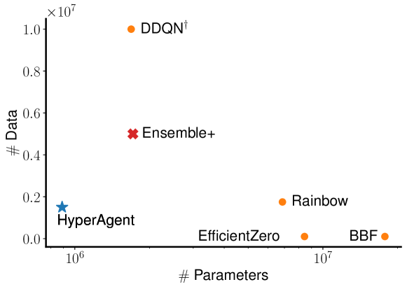
Figure 1: We firstly demonstrate the exceptional efficiency and scalability of HyperAgent, assessed across 26 Atari games using the Interquartile Mean (IQM) metric (Agarwal et al., 2021). This figure investigates the association between necessary training data and the model parameters required to reach human-level performance (quantified by 1.0 IQM) using recent SOTA algorithms. Notably, Ensemble+ (Osband et al., 2018; 2019b) demonstrates limited performance, achieving 0.32 IQM with 5M interaction data, as indicated by ✗. In contrast, HyperAgent, denoted by $\star$, attains an impressive 1.0 IQM with just 1.5M training data. Overall, HyperAgent achieves human-level performance using only 15$\%$ of the training data compared to DDQN^† (Van Hasselt et al., 2016) and employs just 5$\%$ of the model parameters compared to BBF (Schwarzer et al., 2023). Further experimentation underscoring the superiority of HyperAgent are detailed in Section 4.

1 Introduction

Practical reinforcement learning (RL) in complex environments faces challenges such as large state spaces and an increasingly large volume of data. The per-step computational complexity, defined as the computational cost for the agent to make a decision at each interaction step, is crucial. Under resource constraints, any reasonable design of an RL agent must ensure bounded per-step computation, a key requirement for scalability. If per-step computation scales polynomially with the volume of accumulated interaction data, computational requirements will soon become unsustainable, which is untenable for scalability. Data efficiency in sequential decision-making demands that the agent learns the optimal policy with as few interaction steps as possible, a fundamental challenge given the need to balance exploration of the environment to gather more information and exploitation of existing information Thompson (1933); Lai & Robbins (1985); Thrun (1992). Scalability and efficiency are both critical for the practical deployment of RL algorithms in real-world applications with limited resources. There appears to be a divergence between the development of practical RL algorithms, which mainly focus on scalability and computational efficiency, and RL theory, which prioritizes data efficiency, to our knowledge. This divergence raises an important question:

Can we design a practically efficient RL agent with provable guarantees on efficiency and scalability?

1.1 Key Contributions

This work affirmatively answers the posed question by introducing a novel RL agent, HyperAgent. Our main contributions are highlighted below:

• Practical Efficiency: We establish the scalability and efficiency of the HyperAgent algorithm in challenging environments. Specifically, in the Deep Sea exploration environment (Osband et al., 2019a), HyperAgent solves problems up to size $100\times 100$ with optimal episode complexity. Furthermore, on the Atari benchmark suite (Bellemare et al., 2013), HyperAgent achieves human-level performance using only $15\%$ of the data required by DDQN^† (Double-DQN, Van Hasselt et al. (2016)) ($1.5$M interactions) and with only $5\%$ of the network parameters compared to BBF (Bigger, Better, Faster, Schwarzer et al. (2023)), demonstrating significant improvements in data and computational efficiency.

• Algorithmic Simplicity: HyperAgent’s implementation is straightforward, requiring only the addition of a single module to the conventional Double-DQN framework and a minor modification for action selection. This simplicity contrasts with state-of-the-art methods for the Atari benchmarks, which often rely on multiple complex algorithmic components and extensive tuning. The added module facilitates efficient incremental posterior approximation and TS-type action selection, extending DQN-type function approximation in RL beyond conventional approaches.

• Provable Guarantees: We prove that HyperAgent achieves sublinear regret in a tabular, episodic setting with only $\tilde{O}(\log K)$ per-step computation over $K$ episodes, underscoring its scalability and efficiency. This performance is supported by a sequential posterior approximation technique, central to our analysis (Lemma 5.1). This is made possible by the first probability tool for sequential random projection, an extension of the Johnson-Lindenstrauss lemma, which is significant in its own right.

HyperAgent sets a new standard in the design of RL agents, effectively bridging the theoretical and practical aspects of reinforcement learning in complex, large-scale environments.

	Practice in General FA			$(LB)~{}\Omega(\sqrt{H^{3}SAK})$        Theory in Tabular
Alg$\downarrow$ Metric$\rightarrow$	Tract’	Incre’	Effici’	Regret	Per-step Comp’
PSRL	✗	✗	✗	$(B\Re)$ $\tilde{O}(H^{2}\sqrt{SAK})$	$O(S^{2}A)$
Bayes-UCBVI	✗	✗	✗	$(F\Re)$ $\tilde{O}(\sqrt{H^{3}SAK})$	$O(S^{2}A)$
RLSVI	✓	✗	✗	$(B\Re)$ $\tilde{O}(H^{2}\sqrt{SAK})$	$O(S^{2}A)$
Ensemble+	✓	✓	⚫	N/A	N/A
LMC-LSVI	✓	✓	⚫	$(F\Re)$ $\tilde{O}(H^{2}\sqrt{S^{3}A^{3}K})$	✗ $\tilde{O}({\color[rgb]{1,0,0}K}SA+S^{2}A)$
HyperAgent	✓	✓	✓	$(B\Re)$ $\tilde{O}(H^{2}\sqrt{SAK})$	✓ ${O}({\color[rgb]{0.00,0.50,0.00}\log(K)}{SA}+S^{2}A)$

Table 1: Efficiency and Scalability Comparison of Reinforcement Learning (RL) Algorithms: PSRL (Osband & Van Roy, 2017), RLSVI (Osband et al., 2019b), Ensemble+ (Osband et al., 2018; 2019b), Bayes-UCBVI (Tiapkin et al., 2022), LMC-LSVI (Anonymous, 2024), and our HyperAgent. The first column lists the algorithm names. Columns two to four assess whether each algorithm is tractable, incremental, and efficient with general function approximation (FA), respectively. Columns five and six present the regret bound and per-step computational cost in finite horizon, time-inhomogeneous, tabular RL settings, considering the number of states ($S$), actions ($A$), horizons ($H$), and episodes ($K$). Under resource constraints, an RL agent is deemed scalable if its per-step computational complexity does not exceed $\log(K)$ order. Symbols: $(LB)$ denotes minimax lower bound, $(F\Re)$ denotes Frequentist regret, $(B\Re)$ denotes Bayesian regret, ✓ indicates satisfactory results, ✗ indicates unsatisfactory results, and ⚫ represents intermediate outcomes. This comparison underscores the relative strengths and areas for improvement across different RL strategies, with a particular focus on their adaptability to large-scale and complex environments.

1.2 Related works

Computation-first.

The modern development of practical RL algorithms provides scalable solutions to the challenges posed by large state spaces and the increasing size of interaction data under resource constraints. These algorithms’ per-step computation complexity (1) does not scale polynomially with the problem size, thanks to function approximation techniques (Bertsekas & Tsitsiklis, 1996; Mnih et al., 2015); and (2) does not scale polynomially with the increasing size of interaction data, due to advancements in temporal difference learning (Sutton & Barto, 2018), Q-learning (Watkins & Dayan, 1992), and incremental SGD with finite buffers (Mnih et al., 2015). Despite these advances, achieving efficiency in modern RL, especially for real-world applications, remains challenging (Lu et al., 2023). To address data efficiency, recent deep RL algorithms have incorporated increasingly complex heuristic and algorithmic components, such as DDQN (Van Hasselt et al., 2016), Rainbow (Hessel et al., 2018), EfficientZero (Ye et al., 2021), and BBF (Schwarzer et al., 2023). However, these algorithms lack theoretical efficiency guarantees; for example, BBF employs $\varepsilon$-greedy exploration, which is provably data inefficient, requiring exponentially many samples (Kakade, 2003; Strehl, 2007; Osband et al., 2019b; Dann et al., 2022). Furthermore, their practical efficiency often falls short due to high per-step computational costs, exemplified by BBF’s use of larger networks and more complex components that require careful tuning and may challenge deployment in real-world settings. Further discussions can be found in Appendix A and Table 3.

Data-first Exploration.

Efficient exploration in reinforcement learning hinges on decisions driven not only by expectations but also by epistemic uncertainty (Russo et al., 2018; Osband et al., 2019b). Such decisions are informed by immediate and subsequent observations over a long horizon, embodying the concept of deep exploration (Osband et al., 2019b). Among the pivotal exploration strategies in sequential decision-making is Thompson Sampling (TS), which bases decisions on a posterior distribution over models, reflecting the degree of epistemic uncertainty (Thompson, 1933; Strens, 2000; Russo et al., 2018). In its basic form, TS involves sampling a model from the posterior and selecting an action that is optimal according to the sampled model. However, exact posterior sampling remains computationally feasible only in simple environments—like Beta-Bernoulli and Linear-Gaussian Bandits, as well as tabular MDPs with Dirichlet priors over transition probability vectors—where conjugacy facilitates efficient posterior updates (Russo et al., 2018; Strens, 2000).

To extend TS to more complex environments, approximations are indispensable (Russo et al., 2018), encompassing not just function approximation for scalability across large state spaces, but also posterior approximation for epistemic uncertainty estimation beyond conjugate scenarios. Addressing the absence of conjugacy in transition and reward models, value-based TS schemes have been proposed (Zhang, 2022; Dann et al., 2021; Zhong et al., 2022), albeit grappling with computational intractability. Randomized Least-Squares Value Iteration (RLSVI) represents another value-based TS approach, aiming to approximate posterior sampling over the optimal value function without explicitly representing the distribution. This method achieves tractability for value function approximation by introducing randomness through perturbations, thus facilitating deep exploration and enhancing data efficiency (Osband et al., 2019b).

Despite avoiding explicit posterior maintenance, RLSVI demands significant computational effort to generate new point estimates for each episode through independent perturbations and solving the perturbed optimization problem anew, without leveraging previous computations for incremental updates. Consequently, while RLSVI remains feasible under value function approximation, its scalability is challenged by growing interaction data, a limitation shared by subsequent methods like LSVI-PHE (Ishfaq et al., 2021).

Exploration strategies such as ”Optimism in the Face of Uncertainty” (OFU) (Lai & Robbins, 1985) and Information-Directed Sampling (IDS) (Russo & Van Roy, 2018) also play crucial roles. OFU, efficient in tabular settings, encompasses strategies from explicit exploration in unknown states ($E^{3}$, Kearns & Singh (2002)) to bonus-based and bonus-free optimistic exploration (Jaksch et al., 2010; Tiapkin et al., 2022). However, OFU and TS encounter computational hurdles in RL with general function approximation, leading to either intractability or unsustainable resource demands as data accumulates (Jiang et al., 2017; Jin et al., 2021; Du et al., 2021; Foster et al., 2021; Liu et al., 2023; Wang et al., 2020; Agarwal et al., 2023). IDS, while statistically advantageous and tractable in multi-armed and linear bandits, lacks feasible solutions for RL problems in tabular settings (Russo & Van Roy, 2018).

Bridging the Gap.

The divergence between theoretical and practical realms in reinforcement learning (RL) is expanding, with theoretical algorithms lacking practical applicability and practical algorithms exhibiting empirical and theoretical inefficiencies. Ensemble sampling, as introduced by Osband et al. (2016; 2018; 2019b), emerges as a promising technique to approximate the performance of Randomized Least Squares Value Iteration (RLSVI). Further attempts such as Incre-Bayes-UCBVI and Bayes-UCBDQN (Tiapkin et al., 2022) incorporate ensemble-based empirical bootstraps to approximate Bayes-UCBVI, aiming to bridge this gap. These methods maintain multiple point estimates, updated incrementally, essential for scalability. However, the computational demand of managing an ensemble of complex models escalates, especially as the ensemble size must increase to accurately approximate complex posterior distributions (Dwaracherla et al., 2020; Osband et al., 2023a; Li et al., 2022a; Qin et al., 2022).

An alternative strategy involves leveraging a hypermodel (Dwaracherla et al., 2020; Li et al., 2022a) or epistemic neural networks (ENN) (Osband et al., 2023a; b) to generate approximate posterior samples. This approach, while promising, demands a representation potentially more intricate than simple point estimates. The computational overhead of these models, including ensembles, hypermodels, and ENNs, remains theoretically underexplored. Concurrently, LMC-LSVI (Anonymous, 2024), which represents an approximation to Thompson Sampling via Langevin Monte Carlo (LMC) (Russo et al., 2018; Dwaracherla & Van Roy, 2020; Xu et al., 2022), offers a theoretically backed, practically viable deep RL algorithm for a specific class of MDPs. Nevertheless, the per-step computation for LMC-LSVI scales with $\tilde{O}(K)$, where $K$ is the number of episodes, challenging its scalability under constrained resources.

2 Preliminary

2.1 Reinforcement Learning

We consider the episodic RL setting in which an agents interacts with a unknown environment over a sequence of episodes. We model the environment as a Markov Decision Problem (MDP) ${\mathcal{M}}=\left(\mathcal{S},\mathcal{A},P,r,s_{\operatorname{terminal}},\rho\right)$, where $\mathcal{S}$ is the state space, $\mathcal{A}$ is the action space, $\operatorname{terminal}\in\mathcal{S}$ is the terminal state, and $\rho$ is the initial state distribution. For each episode, the initial state $S_{0}$ is drawn from the distribution $\rho$. At each time step $t=1,2,\ldots$ within an episode, the agent observes a state $S_{t}\in\mathcal{S}$. If $S_{t}\neq s_{\operatorname{terminal}}$, the agent selects an action $A_{t}\in\mathcal{A}$, transits to a new state $S_{t+1}\sim P\left(\cdot\mid S_{t},A_{t}\right)$, with reward $R_{t+1}=r(S_{t},A_{t},S_{t+1})$. An episode terminates once the agent arrives at the terminal state. Let $\tau$ be the termination time of a generic episode, i.e., $S_{\tau}=s_{\operatorname{terminal}}$. To illustrate, denote the sequence of observations in episode $k$ by $\mathcal{O}_{k}=\left(S_{k,t},A_{k,t},R_{k,t+1},S_{k,t+1}\right)_{t=0}^{\tau_{k}-1}$ where $S_{k,t},A_{k,t},R_{k,t+1}$ are the state, action, reward at the $t$-th time step of the $k$-th episode and $\tau_{k}$ is the termination time at episode $k$. We denote the history of observations made prior to episode $k$ by $\mathcal{H}_{k}=\left(\mathcal{O}_{1},\ldots,\mathcal{O}_{k-1}\right)$.

A policy $\pi:\mathcal{S}\rightarrow\mathcal{A}$ maps a state $s\in\mathcal{S}$ to an action $a\in\mathcal{A}$. For each MDP ${\mathcal{M}}$ with state space $\mathcal{S}$ and action space $\mathcal{A}$, and each policy $\pi$, we define the associated state-action value function as: $Q_{\mathcal{M}}^{\pi}(s,a):=\mathbb{E}_{{\mathcal{M}},\pi}[\sum_{t=1}^{\tau}R_{t}\mid S_{0}=s,A_{0}=a]$ where the subscript $\pi$ next under the expectation is a shorthand for indicating that actions over the whole time periods are selected according to the policy $\pi$. Let $V_{\mathcal{M}}^{\pi}(s):=Q_{\mathcal{M}}^{\pi}(s,\pi(s))$. We say a policy $\pi^{\mathcal{M}}$ is optimal for the MDP ${\mathcal{M}}$ if $\pi^{\mathcal{M}}(s)\in\arg\max_{\pi}V_{\mathcal{M}}^{\pi}(s)$ for all $s\in\mathcal{S}$. To simplify the exposition, we assume that under any MDP ${\mathcal{M}}$ and policy $\pi$, the termination time $\tau<\infty$ is finite w.p. $1$.

The agent is given knowledge about $\mathcal{S},\mathcal{A},r,s_{\operatorname{terminal}}$, and $\rho$, but is uncertain about $P$. The unknown MDP ${\mathcal{M}}$, together with the unknown transition function $P$, are modeled as random variables with a prior belief. The agent’s behavior is governed by the agent policy $\pi_{\operatorname{agent}}=(\pi_{k})_{k=1}^{K}$ which uses the history $\mathcal{H}_{k}$ to select a policy $\pi_{k}=\operatorname{agent}(\mathcal{S},\mathcal{A},r,\mathcal{H}_{k})$ for the $k$-th episode. The design goal of RL algorithm is to maximize the expected total reward up to episode $K$: $\mathbb{E}[\sum_{k=1}^{K}\sum_{t=1}^{\tau_{k}}R_{k,t}\mid{\mathcal{M}},\pi_{\operatorname{agent}}]$, which is equivalent to $\mathbb{E}[\sum_{k=1}^{K}V_{{\mathcal{M}}}^{\pi_{k}}(s_{k,0})\mid{\mathcal{M}},\pi_{\operatorname{agent}}]$. Note that the expectations are over the randomness from stochastic transitions $P(\cdot\mid\cdot)$ under the given MDP ${\mathcal{M}}$, and the algorithmic randomization introduced by $\operatorname{agent}$. The expectation in the former one is also over the random termination time $\tau_{k}$.

2.2 Hypermodel

As maintaining the degree of uncertainty (Russo et al., 2018) is crucial for data-efficient sequential decision-making, we build RL agents based on the hypermodel framework (Li et al., 2022a; Dwaracherla et al., 2020; Osband et al., 2023a). The Hypermodel, a function parameterized by $\theta$, is designed to efficiently adapt and make decisions through its structure $(f_{\theta},P_{\xi})$. It takes an input $x\in\mathbb{R}^{d}$ and a random index $\xi\sim P_{\xi}$ from a fixed reference distribution, producing an output $f_{\theta}(x,\xi)$ that reflects a sample from the approximate posterior, measuring the degree of uncertainty. The variation in the Hypermodel’s output with $\xi$ captures the model’s degree of uncertainty about $x$, providing a dynamic and adaptable approach to uncertainty representation. This design, combining a trainable parameter $\theta$ with a constant reference distribution $P_{\xi}$, allows the Hypermodel to adjust its uncertainty quantification over time, optimizing its performance and decision-making capabilities in dynamic environments. For example, a special case of linear hypermodel $f_{\theta}(x,\xi)=\langle x,\mu+A\xi\rangle$ with $\theta=(A\in\mathbb{R}^{d\times M},\mu\in\mathbb{R}^{d})$ and $P_{\xi}=N(0,I_{M})$ is essentially Box-Muller transformation. One could sample from linear-Gaussian model $N(x^{\top}\mu,x^{\top}\Sigma x)$ from linear hypermodel if $AA^{\top}=\Sigma$. Another special case is ensemble sampling: with a uniform distribution $P_{\xi}=\mathcal{U}(e_{1},\ldots,e_{M})$ and and an ensemble of models $\theta=A=[\tilde{\theta}_{1},\ldots,\tilde{\theta}_{M}]\in\mathbb{R}^{d\times M}$ s.t. $\tilde{\theta}_{m}\sim N(\mu,\Sigma)$, one can uniformly sample from these ensembles by a form of hypermodel $f_{\theta}(x,\xi):=\langle x,A\xi\rangle$. In general, the hypermodel $f_{\theta}(\cdot)$ can be any function approximators, e.g. neural networks, transforming the reference distribution $P_{\xi}$ to arbitrary distribution. We adopt a class of hypermodel that can be represented as an additive function of a learnable function and a fixed prior model,

$$\underbrace{f_{\theta}(x,\xi)}_{\textbf{``Posterior'' Hypermodel}}=\underbrace{f_{\theta}^{L}(x,\xi)}_{{\textbf{Learnable function}}}+\underbrace{f^{P}(x,\xi)}_{{\textbf{Fixed prior model}}}$$ (1)

The prior model $f^{P}$ represents the prior bias and prior uncertainty, and it has NO trainable parameters. The learnable function is initialized to output value near zero and is then trained by fitting the data. The resultant sum $f_{\theta}(x,\cdot)$ produces reasonable predictions for all probable values of $\xi$, capturing epistemic uncertainty. Similar decomposition in Equation 1 is also used in (Dwaracherla et al., 2020; Li et al., 2022a; Osband et al., 2023a). We will discuss the hypermodel designed in our HyperAgent in Section C.3.1 and clarify the critical differences and advantages compared with prior works in Section C.3.2.

3 Algorithm design

We now develop a novel DQN-type framework for large-scale complex environment, called HyperAgent. (1) It maintains hypermodels to maintain a probability distribution over the action-value function and aims to approximate the posterior distribution of $Q^{*}:=Q^{\pi^{*}}_{M}$. (2) With a SGD-type incremental mechanism, HyperAgent can update the hypermodel to efficiently track the approximate posterior over $Q^{*}$ without leveraging any conjugate property as it encounters more data, and can be implemented as simple as DQN. (3) HyperAgent’s index sampling schemes on action selections and target computation enpowers TS-type efficient exploration with general function approximation.

The hypermodel in this context is a function $f_{\theta}:\mathcal{S}\times\mathcal{A}\times\Xi\rightarrow\mathbb{R}$ parameterized by $\theta\in\Theta$, and $\Xi$ is the index space. Hypermodel is then trained by minimizing the loss function motivated by fitted Q-iteration (FQI), a classical method (Ernst et al., 2005) for batch-based value function approximation with a famous online extension called DQN (Mnih et al., 2015). HyperAgent selects the action based on sampling indices from reference distribution $P_{\xi}$, and then takes the action with the highest value from hypermodels applying these indices, which we call index sampling action selection. This can be viewed as a value-based approximate TS. Alongside the incremental learning process, HyperAgent maintains two hypermodels, one for the current value function $f_{\theta}$ and the other for the target value function $f_{\theta^{-}}$. HyperAgent also maintains a buffer of transitions ${D}=\{(s,a,r,s^{\prime},{\mathbf{z}})\}$, where ${\mathbf{z}}\in\mathbb{R}^{M}$ is the algorithm-generated perturbation random vector sampled from the perturbation distribution $P_{{\mathbf{z}}}$. For a transition tuple $d=(s,a,r,s^{\prime},{\mathbf{z}})\in D$ and given index $\xi$, the temporal difference (TD) loss is

$$\ell^{\gamma,\sigma}(\theta;\theta^{-},{\bm{\xi}}^{-},\xi,d)=(f_{\theta}(s,a,\xi)-(r+\sigma\xi^{\top}{\mathbf{z}}+\gamma\max_{a^{\prime}\in\mathcal{A}}f_{\theta^{-}}(s^{\prime},a^{\prime},{\bm{\xi}}^{-}(s^{\prime}))))^{2},$$ (2)

where $\theta^{-}$ is the target parameters, and the $\sigma$ is a hyperparameter to control the std of algorithmic perturbation. The target index sampling scheme is that ${\bm{\xi}}^{-}(s)\sim P_{\xi}$ for each $s\in\mathcal{S}$, all of which are independent with the given index $\xi$. HyperAgent update the hypermodel by minimizing the loss

$$L^{\gamma,\sigma,\beta}(\theta;\theta^{-},{\bm{\xi}}^{-},D)=\mathbb{E}_{\xi\sim P_{\xi}}[\sum_{d\in D}\frac{1}{|D|}\ell^{\gamma,\sigma}(\theta;\theta^{-},{\bm{\xi}}^{-},\xi,d)]+\frac{\beta}{|D|}{\|\theta\|}^{2}$$ (3)

where $\beta\geq 0$ is for prior regularization. We optimize the loss function Equation 3 using SGD with a mini-batch of data $\tilde{D}$ and a batch of indices $\tilde{\Xi}$ from $P_{\xi}$. That is, we take gradient descent w.r.t. the sampled loss

$$\tilde{L}(\theta;\theta^{-},{\bm{\xi}}^{-},\tilde{D})=\frac{1}{|\tilde{\Xi}|}\sum_{\xi\in\tilde{\Xi}}\sum_{d\in\tilde{D}}\frac{1}{|\tilde{D}|}\ell^{\gamma,\sigma}(\theta;\theta^{-},{\bm{\xi}}^{-},\xi,d)+\frac{\beta}{|D|}\|\theta\|^{2}$$ (4)

We summarize the HyperAgent algorithm: At each episode $k$, HyperAgent samples an index mapping ${\bm{\xi}}_{k}$ from the reference distribution $P_{\xi}$ and then take action by maximizing the associated hypermodel $f_{\theta}(\cdot,a,{\bm{\xi}}_{k}(\cdot))$. HyperAgent maintains a replay buffer of transitions ${D}$, which is used to sample a mini-batch of data $\tilde{D}$ for training the hypermodel incrementally; and updates the main parameters $\theta$ in each episode according to Equation 4, with the target parameters $\theta^{-}$ periodically updated to $\theta$.

Algorithm 1 HyperAgent Framework

1:  Input: Initial parameter $\theta_{\operatorname{init}}$, hypermodel $f_{\theta}(s,a,\xi)$ with reference dist. $P_{\xi}$ and perturbation dist. $P_{{\mathbf{z}}}$.

2:  Init. $\theta=\theta^{-}=\theta_{\operatorname{init}}$, train step $j=0$ and $\operatorname{buffer}$ $D$

3:  for each episode $k=1,2,\ldots$ do

4:     Sample index mapping ${\bm{\xi}}_{k}\sim P_{\xi}$

5:     Set $t=0$ and Observe $S_{k,0}\sim\rho$

6:     repeat

7:        Select $A_{k,t}=\arg\max_{a\in\mathcal{A}}{f}_{\theta}(S_{k,t},a,{{\bm{\xi}}_{k}}(S_{k,t}))$

8:        Observe $S_{k,t+1}$ from environment and $R_{k,t+1}=r(S_{k,t},A_{k,t},S_{k,t+1})$.

9:        Sample perturbation random vector ${\mathbf{z}}_{k,t+1}\sim P_{{\mathbf{z}}}$

10:        $D$.add$((S_{k,t},A_{k,t},R_{k,t+1},S_{k,t+1},{{\mathbf{z}}_{k,t+1}}))$

11:        Increment step counter $t\leftarrow t+1$

12:        $\theta,\theta^{-},j\leftarrow\hyperref@@ii[alg:update-dqn]{\texttt{update}}(D,\theta,\theta^{-},{\bm{\xi}}^{-}={\bm{\xi}}_{k},t,j)$

13:     until $S_{k,t}=s_{\operatorname{terminal}}$

14:  end for

The primary benefits and motivations include straightforward implementation as a plug-and-play alternative to DQN-type methods. Additionally, it provides enhanced features such as computation-efficient sequential posterior approximation and TS-type intelligent exploration, thereby improving data efficiency. Extending actor-critic type deep reinforcement learning algorithms to incorporate similar advantages as in HyperAgent can be readily achieved.

4 Empirical studies

This section assesses the exceptional efficiency and scalability of HyperAgent. The results on DeepSea underscore its superior data and computation efficiency, requiring minimal interactions to learn the optimal policy. Its scalability is demonstrated by successfully handling substantial state spaces up to $100^{2}$. We further evaluate HyperAgent using Atari games, where it excels in processing continuous state spaces with pixels and achieves human-level performance, considering remarkable data and computation efficiency. We provide reproduction details in Appendix B.

4.1 Computational results for deep exploration

Environment.

We demonstrate the exploration effectiveness and scalability of HyperAgent utilizing DeepSea, a reward-sparse environment that demands deep exploration (Osband et al., 2019a; b). Detailed descriptions for DeepSea can be found in Section B.3.

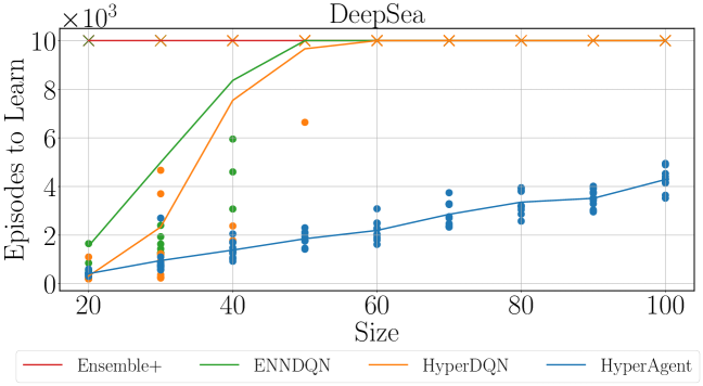
Figure 2: Experiment results on DeepSea. The evaluation metric $\operatorname{Episodes~{}to~{}Learn}(N):=\operatorname{avg}\{K|\bar{R}_{K}\geq 0.99\}$ indicates the number of episodes needed to learn the optimal policy in DeepSea with size $N$. The $\bar{R}_{K}$ represents the return obtained by the agent after $K$ episodes of interaction and it is calculated by averaging over 100 evaluations. The crossmark ✗ indicates that the algorithm could not solve the problem within $10^{4}$ episodes. We set the index dimension to 4 for ENNDQN, HyperDQN and HyperAgent, and the number of ensemble networks to 4 for Ensemble+. We conduct experiments for each algorithm using 10 different initial random seeds, with each result displayed as a distinct point in the figure. The line represents the average result across these 10 seeds.

Comparative analysis.

Based on the structure of DeepSea with size $N$, i.e., $N\times N$ states, the proficient agent can discern an optimal policy within $\Theta(N)$ episodes (Osband et al., 2019b), since it learns to move right from one additional cell along the diagonal in each episode. We compare HyperAgent with several baselines: Ensemble+ (Osband et al., 2018; 2019b), HyperDQN (Li et al., 2022a), and ENNDQN Osband et al. (2023b), which also claimed deep exploration ability. As depicted in Figure 2, HyperAgent outperforms other baselines, showcasing its exceptional data efficiency. It is the only and first deep RL agent learning the optimal policy with optimal episodes complexity ${\Theta}(N)$. Moreover, HyperAgent offers the advantage of computation efficiency as its output layer (hypermodel) maintains constant parameters when scaling up the problem. In contrast, ENNDQN requires a greater number of parameters as the problem’s scale increases, due to the inclusion of the original state as one of the inputs to the output layer (see Section C.3.2). For instance, in DeepSea with size 20, HyperAgent uses only $5\%$ of the parameters required by ENNDQN, showcasing its computation efficiency.

Through more ablation studies on DeepSea in Appendix E, we offer a comprehensive understanding of HyperAgent, including validation for theoretical insights in Section 5, index sampling schemes and sampling-based approximation in Section 3, and comparison with structures within the hypermodel framework in Section 2.2.

4.2 Results on Atari benchmark

Baselines.

We further assess the data and computation efficiency on the Arcade Learning Environment (Bellemare et al., 2013) using IQM (Agarwal et al., 2021) as the evaluation criterion. An IQM score of 1.0 indicates that the algorithm performs on par with humans. We examine HyperAgent with several baselines: DDQN^† (Van Hasselt et al., 2016), Ensemble+ (Osband et al., 2018; 2019b), Rainbow (Hessel et al., 2018), DER (Van Hasselt et al., 2019), HyperDQN (Li et al., 2022a), BBF (Schwarzer et al., 2023) and EfficientZero (Ye et al., 2021). Following the established practice in widely accepted research (Kaiser et al., 2019; Van Hasselt et al., 2019; Ye et al., 2021), the results are compared on 26 Atari games.

Overall results.

Figure 1 illustrates the correlation between model parameters and training data for achieving human-level performance. HyperAgent attains human-level performance with minimal parameters and relatively modest training data, surpassing other methods. Notably, neither DER nor HyperDQN can achieve human-level performance within 2M training data (refer to Appendix F). While several algorithms, such as NoisyNet (Fortunato et al., 2017) and OB2I (Bai et al., 2021), have demonstrated success with Atari games, we avoid redundant comparisons as HyperDQN has consistently outmatched their performance.

Method	IQM	Median	Mean
DDQN†	0.13 (0.11, 0.15)	0.12 (0.07, 0.14)	0.49 (0.43, 0.55)
DDQN(ours)	0.70 (0.69, 0.71)	0.55 (0.54, 0.58)	0.97 (0.95, 1.00)
HyperAgent	1.22 (1.15, 1.30)	1.07 (1.03, 1.14)	1.97 (1.89, 2.07)

Table 2: Performance profiles of HyperAgent. The data in parentheses represent the 95% confidence interval.

Ablation study.

Table 2 displays the comprehensive results of HyperAgent across 26 Atari games. To demonstrate the superior performance of HyperAgent stemming from our principled algorithm design rather than the fine-tuning of hyper-parameters, we developed our version of DDQN, referred to as DDQN(ours). This implementation mirrors the hyper-parameters and network structure (except for the last layer) of HyperAgent. The comparative result with vanilla DDQN^† Hessel et al. (2018) indicates that (1) DDQN(ours) outperforms DDQN^† due to hyperparameters adjustments, and (2) HyperAgent exhibits superior performance compared to DDQN(ours), owing to the inclusion of an additional hypermodel, index sampling schemes and incremental mechanism that facilitate deep exploration. It is worth noting that we also applied an identical set of hyper-parameters across all 55 Atari games (refer to Appendix F), where HyperAgent achieves top performance in 31 out of 55 games, underscoring its robustness and scalability.

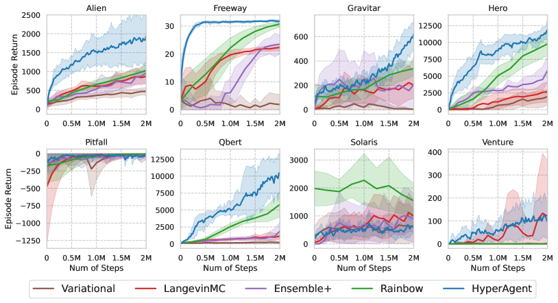
Figure 3: Comparative results of various posterior approximation methods on 8 hardest exploration games.

Exploration on Atari.

We illustrate the exceptional exploration efficiency of HyperAgent on the 8 most challenging exploration Atari games (Bellemare et al., 2016) through a comparison with algorithms employing approximate posterior sampling, such as variational approximation (SANE, Aravindan & Lee (2021)), Langevin Monte-Carlo (AdamLMCDQN, Ishfaq et al. (2023)) and ensemble method (Ensemble+, Osband et al. (2018; 2019b)). In contrast, HyperAgent employs the hypermodel to efficiently and accurately approximate posterior, as a consequence, achieving more efficient deep exploration. As shown in Figure 3, HyperAgent can achieve the best or comparable performance to other baselines in 7 out of 8 games, demonstrating its efficiency and scalability.

5 Theoretical insights and analysis

In this section, we explain the algorithmic insight behind the HyperAgent and how it achieves efficient sequential posterior approximation and deep exploration via incremental update without reliance on conjugacy. For clarity of explanation, let us describe the HyperAgent with tabular function representations.

Tabular HyperAgent.

Let the hypermodel $f_{\theta}(s,a,\xi)=\mu_{sa}+m_{sa}^{\top}\xi+\mu_{0,sa}+\sigma_{0}{\mathbf{z}}_{0,sa}^{\top}\xi$ where $\theta=(\mu\in\mathbb{R}^{|\mathcal{S}||\mathcal{A}|},m\in\mathbb{R}^{|\mathcal{S}||\mathcal{A}|\times M})$ are the parameters to be learned, and ${\mathbf{z}}_{0,sa}\in\mathbb{R}^{M}$ is a random vector from $P_{{\mathbf{z}}}$ and $\mu_{0,sa},\sigma_{0}$ is a prior mean and prior variance for each $(s,a)$. The regularizer in Equation 3 becomes $\beta\|\theta\|^{2}=\beta\sum_{s,a}\left(\mu_{sa}^{2}+\|m_{sa}\|^{2}\right)$. Let $E_{k}={0,1,\ldots,\tau_{k}-1}$ denotes the time index in episode $k$ and $E_{k,sa}=\{t:(S_{k,t},A_{k,t})=(s,a),t\in E_{k}\}$ record the time index the agent encountered $(s,a)$ in the $k$-th episode. Assume $T=\sum_{k=1}^{K}|E_{k}|$ total interactions encountered within $K$ episodes. Let $N_{k,sa}=\sum_{\ell=1}^{k-1}|E_{\ell,sa}|$ denotes the counts of visitation for state-action pair $(s,a)$ prior to episode $k$. For every pair $(s,a)$ with $N_{k,sa}>0$, $\forall s^{\prime}\in\mathcal{S}$, the empirical transition probabilities up to episode $k$ are $\hat{P}_{k,sa}(s^{\prime}):=\sum_{\ell=1}^{k-1}\sum_{t\in E_{\ell}}\frac{\mathds{1}_{(S_{t},A_{t},S_{t+1})=(s,a,s^{\prime})}}{N_{k,sa}}$. For the case $N_{k,sa}=0$, define $\hat{P}_{k,sa}(s^{\prime})=1$ for any selected one $s^{\prime}\in\mathcal{S}$. Let us define a value vector $f_{\theta,{\bm{\xi}}}(s,a):=f_{\theta}(s,a,{\bm{\xi}}(s)),\forall(s,a)\in\mathcal{S}\times\mathcal{A}.$ In episode $k$, HyperAgent will act greedily according the action-value vector $f_{\theta_{k},{\bm{\xi}}_{k}}$ where $\theta_{k}=(\mu_{k},m_{k})$.

Closed-form incremental update.

Initially $\theta_{0}:=(\mu_{0}=\mathbf{0},m_{0}=\mathbf{0})$. Suppose HyperAgent maintains parameters $\theta_{k}^{(0)}:=\theta_{k-1}=(\mu_{k-1},m_{k-1})$, the buffer $D=\mathcal{H}_{k}$ and target noise mapping ${\bm{\xi}}^{-}={\bm{\xi}}_{k}$ at the beginning of the episode $k$. Iteratively solve Equation 3 with $\beta=\sigma^{2}/\sigma_{0}^{2},\theta^{-}=\theta_{k}^{(i)}$ and output $\theta_{k}^{(i+1)}$ from $i=0$ until converging to $\theta_{k}$, tabular HyperAgent would yield the closed-form iterative update rule (1) $m_{k-1}\rightarrow m_{k}$ and (2) $\theta_{k}^{(i)}=(\mu_{k}^{(i)},m_{k})\rightarrow\theta_{k}^{(i+1)}=(\mu_{k}^{(i+1)},m_{k})$. With short notation $\tilde{m}_{k,sa}=m_{k,sa}+\sigma_{0}{\mathbf{z}}_{0,sa}$, for all $(s,a,k)$,

$$\tilde{m}_{k,sa}=\frac{(N_{k-1,sa}+\beta)\tilde{m}_{k-1,sa}+\sum_{t\in E_{k-1,sa}}\sigma{\mathbf{z}}_{\ell,t+1}}{(N_{k,sa}+\beta)}$$ (5)

$$f_{\theta_{k}^{(i+1)},{\bm{\xi}}_{k}}=F^{\gamma}_{k}f_{\theta_{k}^{(i)},{\bm{\xi}}_{k}}$$ (6)

where $F^{\gamma}_{k}$ can be regarded as a stochastic bellman operator induced by HyperAgent in episode $k$: for any $Q$-value function,

$$F_{k}^{\gamma}Q(s,a):=\frac{\beta\mu_{0,sa}+N_{k,sa}(r_{sa}+\gamma V_{Q}^{\top}\hat{P}_{k,sa})}{N_{k,sa}+\beta}+\tilde{m}_{k,sa}^{\top}{\bm{\xi}}_{k}(s),$$ (7)

where $V_{Q}(s):=\max_{a}Q(s,a),\forall s$ is the greedy value w.r.t. $Q$. Equations 5, 6 and 7, whose derivations can be found in Section C.4, are crucial for understanding.

Understanding Equation 5.

This is an incremental update with computation complexity $O(M)$. A key property of hypermodel in HyperAgent is that, with logarithmically small $M$, it can approximate the posterior distribution sequentially in every episodes via incremental update in Equation 5. This is formalized as the following key lemma.

Lemma 5.1 (Sequential posterior approximation).

For $\tilde{m}_{k}$ recursively defined in Equation 5 with ${\mathbf{z}}\sim\mathcal{U}(\mathbb{S}^{M-1})$. For any $k\geq 1$, define the good event of $\varepsilon$-approximation

$$\mathcal{G}_{k,sa}(\varepsilon):=\bigg{\{}\|\tilde{m}_{k,sa}\|^{2}\in\left(\frac{(1-\varepsilon)\sigma^{2}}{N_{k,sa}+\beta},\frac{(1+\varepsilon)\sigma^{2}}{N_{k,sa}+\beta}\right)\bigg{\}}.$$

The joint event $\cap_{(s,a)\in\mathcal{S}\times\mathcal{A}}\cap_{k=1}^{K}\mathcal{G}_{k,sa}(\varepsilon)$ holds w.p. at least $1-\delta$ if $M\simeq\varepsilon^{-2}\log(|\mathcal{S}||\mathcal{A}|T/\delta)$.

A direct observation from Lemma 5.1 is larger $M$ results smaller $\varepsilon$, thus more accurate approximation of posterior variance over $Q^{*}(s,a)$ using their visitation counts and appropriately chosen $\sigma$. Intuitively, more experience at $(s,a)$, less epistemic uncertainty and smaller posterior variance on $Q^{*}(s,a)$. As shown in Section D.1, the difficulty for proving Lemma 5.1 is from the sequential dependence among high-dimensional random variables. It is resolved due to the developed first probability tool (Li, 2024a) for sequential random projection and a new simple and unified analysis of random projection via a high-dimensional version of Hanson-Wright inequality (Li, 2024b). These are novel technical contributions, which maybe of independent interests. Additionally, in the regret analysis, we will show constant approximation $\varepsilon=1/2$ suffices for computation and data efficient deep exploration.

Understanding Equation 7.

As shown in Lemma C.1, the stochastic bellman operator $F_{k}^{\gamma}$ is a contraction mapping and thus guarantee convergence of Equation 6. It differs from the empirical Bellman iteration $V_{Q}^{\top}\hat{{P}}_{k,sa}$ in two ways: (1) there is a slight regularization toward the prior mean $\mu_{0,sa}$, and (2) more importantly, HyperAgent adds noise $w_{k,sa}:=\tilde{m}_{k,sa}^{\top}{\bm{\xi}}_{k}(s)$ to each iteration. For a common choice ${\bm{\xi}}_{k}(s)\sim P_{\xi}:=N(0,I_{M})$, the noise $w_{k,sa}$ is Gaussian distributed conditioned on $\tilde{m}_{k,sa}$. Incorporating the Gaussian noise in the bellman iteration would backpropagate the uncertainty estimates, which is essential to incentives the deep exploration behavior. This is because larger posterior variance of later states with less visitation, shown in Lemma 5.1, will be backpropagated to initial states and induce exploration to few-visited state space. More discussions in Section D.2.

Furthermore, to rigorously justify the algorithmic insight and corresponding benefits, we provide theoretical results for HyperAgent with tabular representation and hyper-parameters for update specified in Table 6. Denote the regret of a policy $\pi_{k}$ over episode $k$ by $\Delta_{k}:={V_{{\mathcal{M}}}^{\pi^{*}}(s_{k,0})-V_{{\mathcal{M}}}^{\pi_{k}}(s_{k,0})},$ where $\pi^{*}$ is an optimal policy for $M$. Maximizing total reward is equivalent to minimizing the expected total regret: $\operatorname{Regret}(K,\operatorname{agent}):=\mathbb{E}\sum_{k=1}^{K}\Delta_{k}.$

Theorem 5.2.

Under Assumptions D.8 and D.9 with $\beta\geq 3$, if the Tabular HyperAgent is applied with planning horizon $H$, and parameters with $(M,\mu_{0},\sigma,\sigma_{0})$ satisfying

$$M=O(1)\cdot\log(SAHK)=\tilde{O}(\log K),$$

$(\sigma^{2}/\sigma_{0}^{2})=\beta$, $\sigma\geq\sqrt{6}H$ and $\min_{sa}\mu_{0,sa}\geq H$, then for all $K\in\mathbb{N}$,

$$\operatorname{Regret}(K,{\hyperref@@ii[alg:hyperagent]{\texttt{HyperAgent}}})\leq 18H^{2}\sqrt{\beta SAK\log_{+}(1+SAHK)}\log_{+}\left(1+{K}/{SA}\right),$$

where $\log_{+}(x)=\max(1,\log(x))$. The per-step computation of HyperAgent is $O(S^{2}A+SAM)$.

Remark 5.3.

The time-inhomogeneous MDP is a common benchmark for regret analysis in the literature, e.g. (Azar et al., 2017; Osband et al., 2019b). For notation unification with Table 1, as explained in Assumption D.8, $|\mathcal{S}|=SH,|\mathcal{A}|=A$ and $\tau=H$ almost surely. The Assumption D.9 is common in the literature of Bayesian regret analysis (Osband et al., 2013; 2019b; Osband & Van Roy, 2017; Lu & Van Roy, 2019). The regret bound $\tilde{O}(H^{2}\sqrt{SAK})$ of HyperAgent matches the best known Bayesian regret bound, say those of RLSVI (Osband et al., 2019b) and PSRL (Osband & Van Roy, 2017), while HyperAgent provide the computation and scalability benefits that RLSVI and PSRL do not have, as discussed in Sections 1 and 1. On the other hand, most practically scalable algorithm, including recent BBF (Schwarzer et al., 2023), uses $\varepsilon$-greedy, which is provably data-inefficient without sublinear regret guarantees in general (Dann et al., 2022). As shown in Table 1, a recent concurrent work claims LMC-LSVI (Anonymous, 2024) is practical and provable but suffer $\tilde{O}(K)$ per-step computational complexity, which is not acceptable under bounded computation resource constraints. Instead, per-step computation of HyperAgent is $\tilde{O}(\log K)$. These comparisons implies HyperAgent is the first provably scalable and efficient RL agent among practically useful ones. Analytical details is in Section D.3. Extension to frequentist regret without Assumption D.9 is direct either using HyperAgent or its variants of optimistic index sampling in Section C.2.

6 Conclusion and future directions

We present an innovative RL framework, HyperAgent, that simplifies, accelerates, and scales the learning process across complex environments. By integrating a hypermodel with index sampling and incremental updates, HyperAgent achieves significant efficiency in data and computation over baselines, which is demonstrated through superior performance in challenging benchmarks like the DeepSea and Atari suites, with minimal computational resources. The framework’s algorithmic simplicity, practical efficiency, and theoretical underpinnings—highlighted by a novel analytical tool for sequential random projection—establish HyperAgent as a pioneering solution that effectively bridges the gap between theoretical rigor and practical application in reinforcement learning, setting new standards for future RL algorithm design.

Intriguing future directions in both practical and theoretical domains is highlighted here. On the practical side, the hypermodel’s compatibility with any feedforward neural network architecture offers seamless integration into a wide array of deep reinforcement learning frameworks, including actor-critic structures and transformer-based large models. This flexibility enhances its utility across various applications, such as healthcare, robotics and large language models (LLMs), and exploring these integrations further could yield significant advancements. Theoretically, the prospect of extending our analysis to include linear, generalized linear, and neural tangent kernel function approximations with SGD update opens up a promising field for future studies. This exploration could deepen our understanding of the underlying mechanisms and improve the model’s efficacy and applicability in complex scenarios, further bridging the gap.

Impact statement

HyperAgent represents a significant step forward in the field of reinforcement learning (RL). Its application could span across multiple sectors including gaming, autonomous vehicles, robotics, healthcare, financial trading, energy production and many more. Given its computation-efficient and data-efficient design, businesses across these sectors could leverage this new technology to make real-time decisions, optimizing for efficiency and desired outcomes, under resource constraints.

Education and research in machine learning (ML) could potentially benefit from this novel framework. As the algorithm is simple to implement, it could facilitate learning and experimentation amongst researchers and students, potentially accelerating advancements in the field. This tool could also become an instrumental part of academic research and corporate R&D, prompting more discoveries and technological breakthroughs in AI.

The proposal of the sequential random projection, a non-trivial martingale extension of the Johnson-Lindenstrauss lemma, could offer new dimensions in the theoretical understanding of random projection in adaptive processes and RL, influencing both fundamental research and practical applications of probability, applied probability and RL across various domains.

The simplicity of the proposed HyperAgent’s implementation could democratize access to RL algorithms, fostering innovation and growth. However, such technology should be accompanied by necessary education in ethical matters to prevent misuse, including privacy violations, unfair decision making, and more.

From an ethical stand-point, the handling of large scale, increasingly accumulated interaction data would require robust policies and protocols, ensuring user privacy and data protection. Its ability to efficiently handle larger data sets may further increase concerns regarding data privacy.

The scalability and performance of HyperAgent could empower smaller organizations and start-ups that might not have access to large computing resources, which could lead to a more level playing field in the technology sector, and encourage the focus on creative innovation over resource gathering.

It’s important to be vigilant about the potential consequences of AI technologies. Autonomous sequential decision-making with RL could unintentionally lead to behavior that in the worst-case could be harmful. There should be checks in place to ensure ethically sound implementation and continuous monitoring of outcomes for fairness, safety and security.

Appendix A Additional discussion on related works

Our work represents sustained and focused efforts towards developing principled RL algorithms that are practically efficient with function approximation in complex environments.

Ensemble-based methods.

Osband & Van Roy (2015); Osband et al. (2016) initiated the bootstrapped ensemble methods, an incremental version of randomized value functions (Wen, 2014), on bandit and deep RL, maintaining an ensemble of point estimates, each being incremental updated. This algorithm design methodology avoid refit a potentially complex model from scratch in the online interactive decision problems. Bayes-UCBVI (Tiapkin et al., 2022) was extended to Incre-Bayes-UCBVI (Tiapkin et al., 2022) using the exact same idea as Algorithm 5 in (Osband & Van Roy, 2015) and then extended to Bayes-UCBDQN (Tiapkin et al., 2022) following BootDQN (Osband et al., 2016). As reported by the author, Bayes-UCBDQN shares very similar performance as BootDQN (Osband et al., 2016) but requires addition algorithmic module on artificially generated pseudo transitions and pseduo targets, which is environment-dependent and challenging to tune in practice as mentioned in appendix G.3 of (Tiapkin et al., 2022). Ensemble+ (Osband et al., 2018; 2019b) introduces the randomized prior function for controlling the exploration behavior in the initial stages, somewhat similar to optimistic initialization in tabular RL algorithm design, facilitate the deep exploration and data efficiency. This additive prior design principle is further employed in a line of works (Dwaracherla et al., 2020; Li et al., 2022a; Osband et al., 2023a; b). For a practical implmentation of LSVI-PHE Ishfaq et al. (2021), it utilizes the optimistic sampling (OS) with ensemble methods as a heuristic combination: it maintains an ensemble of $M$ value networks $\{Q_{i}(s,a),i=1,\ldots,M\}$ and take greedy action according to the maximum value function over $M$ values $Q(s,a)=\max_{i\in[M]}Q_{i}(s,a)$ for action selection and $Q$-target computation. As will be discussed in Section C.2, we propose another index sampling scheme called optimistic index sampling (OIS). OIS, OS and quantile-based Incre-Bayes-UCBVI are related in a high level, all using multiple randomized value functions to form a optimistic value function with high probability, thus leading to OFU-based principle for deep exploration. Critical distinction exists, compared with ensemble-based OS and Incre-Bayes-UCBVI, OIS is computationally much more friendly due to our continuous reference distribution $P_{\xi}$ for sampling as many indices as possible to construct randomized value functions.

Theoretical analysis of ensemble based sampling is rare and difficult. As pointed out by the first correct analysis of ensemble sampling for linear bandit problem (Qin et al., 2022), the first analysis of ensemble sampling in 2017 has technical flaws. The results of Qin et al. (2022) show Ensemble sampling, although achieving sublinear regret in ($d$-dimensional, $T$-steps) linear bandit problems, requires $\tilde{O}(T)$ per-step computation, which is unsatisfied for a scalable agent with bounded resource. Because of the potential challenges, there is currently no theoretical analysis available for ensemble-based randomized value functions across any class of RL problems.

Langevin Monte-Carlo.

Langecin Monte-Carlo (LMC), staring from SGLD (Welling & Teh, 2011), has huge influence in Bayesian deep learning and approximate Bayesian inference. However, as discussed in many literature, e.g. ENN (Osband et al., 2023a), the computational costs of LMC-based inference are prohibitive in large scale deep learning systems. Recent advances show the application of LMC-based posterior inference for sequence decision making, such as LMCTS (Xu et al., 2022) for contextual bandits and LangevinDQN (Dwaracherla & Van Roy, 2020) LMC-LSVI (Anonymous, 2024) for RL problems. As we will discuss in the following, these LMC based TS schemes still suffer scalability issues as the per-step computational complexity would grow unbounded with the increasingly large amount of interaction data.

LMCTS (Xu et al., 2022) provides the first regret bound of LMC based TS scheme in ($d$-dimensional, $T$-steps) linear bandit problem, showing $\tilde{O}(d^{3/2}\sqrt{T})$ regret bound with $\kappa_{t}\log(3\sqrt{2dT\log(T^{3})})$ inner-loop iteration complexity within time step $t$. As discussed in (Xu et al., 2022), the conditional number $\kappa_{t}=O(t)$ in general. For a single iteration in time step $t$, LMC requires $O(d^{2})$ computation for a gradient calculation of loss function: $\nabla L_{t}(\theta)=2(V_{t}\theta-b_{t})$ using notations in Xu et al. (2022); and $O(d)$ computation on noise generation and parameters update (line 5 and 6 in Algorithm 1 Xu et al. (2022)). Additional $dA$ computation comes from greedy action selection among action set $\mathcal{A}$ by first computing rewards with inner product and selecting the maximum. Therefore, the per-step computation complexity of LMCTS is $\tilde{O}(d^{2}T+dA)$, which scales polynomially with increasing number of interactions $T$. LMCTS is not provably scalable under resource constraints.

LMC-LSVI (Anonymous, 2024) apply similar methodologies and analytical tools as LMCTS (Xu et al., 2022), providing $\tilde{O}(d^{3/2}H^{3/2}\sqrt{T})$ regret in the linear MDP ($d$-dimensional feature mappings and $H$-horizons and $K$ episodes where $T=KH$). The inner-loop iteration complexity of LMC within one time step $(k,h)$ of episode $k$ is $2\kappa_{k}\log(4HKd)$ . Similarly, $\kappa_{k}=O(k)$ in general. (1) In the general feature case: For a single iteration in time step $(k,h)$, LMC requires $O(d^{2})$ computation cost for the gradient calculation as from equation (6) of (Anonymous, 2024) and $O(d)$ computation cost for noise generation and parameter update. The per-step computational complexity caused by LMC inner-loops is $O(d^{2}\kappa_{k}\log(4HKd))=O(d^{2}k\log(HKd))$. Additional per-step computation cost in episode $k$ is $\tilde{O}(d^{2}Ak)$, coming from LSVI as discussed in (Jin et al., 2020). Therefore, the per-step computation complexity is $\tilde{O}(d^{2}K\log(HKd)+d^{2}AK)$, scaling polynomially with increasing number of episodes $K$. (2) When consider tabular representation where the feature is one-hot vector with $d=SA$, the per-step computational complexity caused by LMC is $O(SAK\log(SAHK))$ as the covariance matrix is diagonal in the tabular setting. The computation cost by LSVI is now $O(S^{2}A)$ with no dependence on $K$ as we can perform incremental counting and bottom-up dynamic programming in tabular setting. The per-step computational complexity of LMC-LSVI is $O(SAK\log(SAHK)+S^{2}A)$, still scaling polynomially with increasing number of episodes $K$. LMC-LSVI is not provably scalable under resource constraints.

Anonymous (2024) also extends their LMC-LSVI to deep RL setting, with a combination of Adam optimization techniques, resulting the AdamLMCDQN. Naturally, it introduces additional 5 hyper-paramters to tune as shown in Algorithm 2 of (Anonymous, 2024) since they cannot directly use default Adam hyper-parameters due to their algorithms design. In practice, as shown in the appendix of (Anonymous, 2024), AdamLMCDQN uses different hyper-parameters tuned specifically for 8 different Atari environments, which is not a standard practice, showing its deployment difficulty. As shown in Figure 3, our HyperAgent, using a single set of hyper-parameters for every environments, performs much better than AdamLMCDQN in all 8 hardest exploration Atari environments.

Heuristics on noise injection.

For example, Noisy-Net (Fortunato et al., 2017) learns noisy parameters using gradient descent, whereas Plappert et al. (2017) added constant Gaussian noise to the parameters of the neural network. SANE (Aravindan & Lee, 2021) is a variational Thompson sampling approximation for DQNs which uses a deep network whose parameters are perturbed by a learned variational noise distribution. Noisy-Net can be regarded as an approximation to the SANE. While Langevin Monte-Carlo may seem simliar to Noisy-Net (Fortunato et al., 2017; Plappert et al., 2017) or SANE (Aravindan & Lee, 2021) due to their random perturbations of neural network weights in state-action value and target value computation, as well as action selection. Critical differences exist, as noisy networks are not ensured to approximate the posterior distribution (Fortunato et al., 2017) and do not achieve deep exploration (Osband et al., 2018). SANE (Aravindan & Lee, 2021) also lacks rigorous guarantees on posterior approximation and deep exploration.

Discussion on the simplicity and deployment efficiency.

Several works (Hessel et al., 2018; Van Hasselt et al., 2019; Schwarzer et al., 2023) employ a combination of techniques, including dueling networks (Wang et al., 2016), reset strategy (Nikishin et al., 2022), distributional RL (Bellemare et al., 2017), and others, to achieve data efficiency. Some have demonstrated remarkable performance on Atari games. However, integrating multiple techniques makes the algorithms complicated and challenging to apply to various scenarios. It requires careful selection of hyperparameters for each technique. For example, the reset frequency in the reset strategy needs meticulous consideration. Furthermore, combining multiple techniques results in a significant computational cost. For instance, BBF (Schwarzer et al., 2023) designs a larger network with 15 convolutional layers, which has 20 times more parameters than our method. Model-based RL (Kaiser et al., 2019; Schrittwieser et al., 2020; Ye et al., 2021; Hafner et al., 2023) is a widely used approach for achieving data efficiency. However, the performance of these methods is contingent upon the accuracy of the learned predictive model. Furthermore, the learning of predictive models can incur higher computational costs, and employing tree-based search methods with predictive models may not offer sufficient exploration. Other methods (Schwarzer et al., 2020; Laskin et al., 2020; Liu & Abbeel, 2021; Cagatan, 2023) achieve data efficiency by enhancing representation learning. While these approaches perform well in environments with image-based states, they show poorer performance in environments characterized by simple structure yet requiring deep exploration, as seen in DeepSea.

Algorithm	Components
DDQN	incremental SGD with experience replay and target network
Rainbow	(DDQN) + Prioritized replay, Dueling networks, Distributional RL, Noisy Nets.
BBF	(DDQN) + Prioritized replay, Dueling networks, Distributional RL,
	Self-Prediction, Harder resets, Larger network, Annealing hyper-parameters.
HyperAgent	(DDQN) + hypermodel

Table 3: The extra techniques used in different algorithms, e.g. DDQN (Van Hasselt et al., 2016), Rainbow (Hessel et al., 2018), BBF (Schwarzer et al., 2023) and HyperAgent.

Appendix B Reproducibility

In support of other researchers interested in utilizing our work and authenticating our findings, we offer the implementation of HyperAgent at the link https://anonymous.4open.science/r/HyperAgent-0754. This repository includes all the necessary code to replicate our experimental results and instructions on usage. Following this, we will present the evaluation protocol employed in our experiments and the reproducibility of the compared baselines.

B.1 Evaluation protocol

Protocol on DeepSea.

We replicate all experiments on DeeSea using 10 different random seeds. In each experiment run, we evaluate the agent 100 times for every 1000 interactions to obtain the average return. The experiment stops when the average return reaches 0.99, at which point we record the number of interactions used by the agent. We then collect 10 data points (the number of interactions) for a specific problem size $N$, which are then utilized to generate a scatter plot in Figures 2, 7, 8, LABEL:fig:deepsea_ois, 11, 11, 12, 13 and 14. Each point on the curve represents the average over the 10 data points.

Protocol on Atari.

For the experiments on Atari, our training and evaluation protocol follows the baseline works (Mnih et al., 2015; Van Hasselt et al., 2016; Kaiser et al., 2019; Li et al., 2022a) During the training process, we assess the agent 10 times after every 20,000 interactions to calculate the average return at each checkpoint. This allows us to obtain 20 data points for each game at every checkpoint, as we repeat the process with 20 different random seeds. We then compute the mean and 90$\%$ confidence interval range for plotting the learning curve in Figures 3, 19 and 20.

We calculate the best score for each game using the following steps: (1) for each Atari game, the algorithm is performed with 20 different initial random seeds; (2) The program with one particular random seed will produce one best model (the checkpoint with highest average return), leading to 20 different models for each Atari game; (3) We then evaluate all 20 models, each for 200 times; (4) We calculate the average score from these 200 evaluations as the score for each model associated with each seed. (5) Finally, we calculate and report the average score across 20 seeds as the final score for each Atari game. We follow the aforementioned five-step protocol to determine the score for each game outlined in Tables 7 and 9. We then utilize the 20 scores for each of the 26 Atari games to compute the IQM, median, and mean score with 95$\%$ confidence interval for each algorithm as depicted in Tables 2 and 8.

B.2 Reproducibility of baselines

Experiments on DeepSea.

We present our HyperModel and ENNDQN implementation and utilize the official HyperDQN implementation from https://github.com/liziniu/HyperDQN to replicate results. We kindly request the implementation of Ensemble+ from the author of Li et al. (2022a), and they employ the repository at https://github.com/google-deepmind/bsuite for reproduction. We perform ablation studies in DeepSea benchmarks for a comprehensive understanding of HyperAgent in Appendix E.

Experiments on Atari.

We provide our version of DDQN(ours) and replicated the results using a well-known repository (https://github.com/Kaixhin/Rainbow) for DER. We obtained the result data for DDQN^† and Rainbow from https://github.com/google-deepmind/dqn_zoo. As they were based on 200M frames, we extracted the initial 20M steps from these results to compare them with HyperAgent. We acquired the implementation of BBF (https://github.com/google-research/google-research/tree/master/bigger_better_faster) and EfficientZero (https://github.com/YeWR/EfficientZero) from their official repositories, and reached out to the author of Li et al. (2022a) for the results data of Ensemble+ with an ensemble size of 10. For the experiments about exploration on Atari (refer to Figure 3 and Figure 20), we utilized the official implementation (https://github.com/NUS-LID/SANE) to replicate the results of SANE. Additionally, we obtained the raw result data of AdamLMCDQN and LangevinAdam from https://github.com/hmishfaq/lmc-lsvi. In addition to the results shown in the main article, we also provide fine-grained studies on Atari suite in Appendix F.

B.3 Environment Settings

In this section, we describe the environments used in experiments. We firstly use the DeepSea (Osband et al., 2019a; b) to demonstrate the exploration efficiency and scalability of HyperAgent. DeepSea (see Figure 4) is a reward-sparse environment that demands deep exploration (Osband et al., 2019b). The environment under consideration has a discrete action space consisting of two actions: moving left or right. During each run of the experiment, the action for moving right is randomly sampled from Bernoulli distribution for each row. Specifically, the action variable takes binary values of 1 or 0 for moving right, and the action map is different for each run of the experiment. The agent receives a reward of 0 for moving left, and a penalty of $-(0.01/N)$ for moving right, where $N$ denotes the size of DeepSea. The agent will earn a reward of 1 upon reaching the lower-right corner. The optimal policy for the agent is to learn to move continuously towards the right. The sparse rewards and states presented in this environment effectively showcase the exploration efficiency of HyperAgent without any additional complexity.

For the experiments on the Atari games, we utilized the standard wrapper provided by OpenAI gym. Specifically, we terminated each environment after a maximum of 108K steps without using sticky actions. For further details on the settings used for the Atari games, please refer to Table 4.

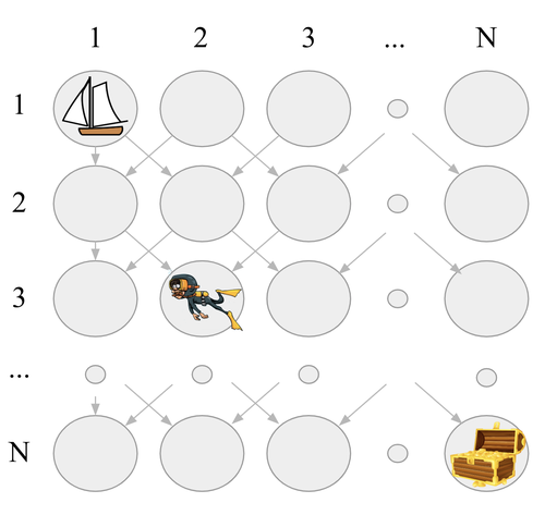
Figure 4: Illustration for DeepSea.

Hyper-parameters	Setting
Grey scaling	True
Sticky action	False
Observation down-sampling	(84, 84)
Frames stacked	4
Action repetitions	4
Reward clipping	[-1, 1]
Terminal on loss of life	True
Max frames per episode	108K

Table 4: Detailed settings for Atari games

Appendix C HyperAgent details

In this section, we describe more details of the proposed HyperAgent. First, we describe the general treatment for the incremental update function (in line 11 of HyperAgent) in the following Algorithm 2 of Section C.1. Then, we provide the details of index sampling schemes in Section C.2. Next, in Section C.3, we provide the implementation details of HyperAgent with deep neural network (DNN) function approximation. We want to emphasize that all experiments done in this article is using Option (1) with DNN value function approximation. In Section C.4, we describe the closed-form update rule (Option (2)) when the tabular representation of the value function is exploited. Note that the tabular version of HyperAgent is only for the clarity of analysis and understanding.

C.1 Incremental update mechanism of HyperAgent

Algorithm 2 update

1:  Input: $\operatorname{buffer}D$, $\theta,\theta^{-},{\bm{\xi}}^{-}$, agent step $t$, train step $j$

2:  if $t\mod\operatorname{training\_freq}=0$ then

3:     repeat

4:         Obtain $\theta$ by optimizing the loss $L^{\gamma,\sigma,\beta}(\theta;\theta^{-},{\bm{\xi}}^{-},D)$ in  Equation 3: – Option (1) with gradient descent w.r.t. the mini-batch sampled loss Equation 4; (HyperAgent) – Option (2) with closed-form update in Equations 5, 6 and 7. (Tabular HyperAgent)

5:        Increment $j\leftarrow j+1$

6:        if  $(j\mod\operatorname{target\_update\_freq})=0$ then

7:            $\theta^{-}\leftarrow\theta$

8:        end if

9:     until  $(j\mod\operatorname{sample\_update\_ratio}\times\operatorname{training\_freq})=0$

10:  end if

11:  Return: $\theta,\theta^{-},j$.

Notice that in update, there are three important hyper-parameters $(\operatorname{target\_update\_freq}$, $\operatorname{sample\_update\_ratio}$, $\operatorname{training\_freq})$, which we will specify in Table 5 the hyper-paramters for practical implementation of HyperAgent with DNN function approximation for all experimental studies; and in Table 6 the hyper-parameters only for regret analysis in finite-horizon tabular RL with fixed horizon $H$. To highlight, We have not seen this level of unification of algorithmic update rules between practice and theoretical analysis in literature!

Hyper-parameters	Atari Setting	DeepSea Setting
weight decay $\beta$	0.01	0
discount factor $\gamma$	0.99	0.99
learning rate	0.001	0.001
mini-batch size $|\tilde{D}|$	32	128
index dim $M$	4	4
# Indices $|\tilde{\Xi}|$ for approximation	20	20
$\sigma$ in Equation 2	0.01	0.0001
$n$-step target	5	1
$\operatorname{target\_update\_freq}$ in update	5	4
$\operatorname{sample\_update\_ratio}$ in update	1	1
$\operatorname{training\_freq}$ in update	1	1
hidden units	256	64
min replay size for sampling	2,000 steps	128 steps
memory size	500,000 steps	1000000 steps

Table 5: Hyper-parameters of HyperAgent. Other hyper-parameters used for Atari suite are the same as Rainbow (Hessel et al., 2018). Note that we utilize a single configuration for all 55 games from Atari suite and a single configuration for DeepSea with varying sizes.

For the approximation of expectation in Equation 3, we sample multiple indices for each transition tuple in the mini-batch and compute the empirical average, as described in Equation 4. Recall that $|\tilde{\Xi}|$ is the number of indices for each state and we set $|\tilde{\Xi}|=20$ as default setting. We have demonstrated how the number of indices $|\tilde{\Xi}|$ impacts our method in Section E.2.

C.2 Index sampling schemes of HyperAgent

We have two options for index sampling schemes for ${\bm{\xi}}_{k}(s)$:

1. State-dependent sampling. As for implementation, especially for continuous or uncountable infinite state space: in the interaction, ${\bm{\xi}}_{k}(s)$ in the line 7 of HyperAgent is implemented as independently sampling $\xi\sim P_{\xi}$ for each encountered state; for the target computation in Equation 2, ${\bm{\xi}}_{k}(s^{\prime})$ is implemented as independently sampling $\xi\sim P_{\xi}$ for each tuple $d=(s,a,r,s^{\prime},{\mathbf{z}})$ in the every sampled mini-batch.

2. State-independent sampling. The implementation of state-independent ${\bm{\xi}}_{k}(s)=\xi_{k}$ is straightforward as we independently sample $\xi_{k}$ in the beginning of each episode $k$ and use the same $\xi_{k}$ for each state $s$ encountered in the interaction and for each target state $s^{\prime}$ in target computation.

In our implementation by default, HyperAgent employs the state-independent ${\bm{\xi}}$ for action selection and utilizes state-dependent ${\bm{\xi}}$ for $Q$-target computation. The ablation results in Section E.1 demonstrate that these distinct index sampling schemes for ${\bm{\xi}}$ yield nearly identical performance.

Optimistic index sampling.

To make agent’s behavior more optimistic with more aggresive deep exploration, in each episode $k$, we can sample $N_{\operatorname{OIS}}$ indices $\xi_{k,1},\ldots,\xi_{k,N_{\operatorname{OIS}}}$ and take the greedy action according to the associated hypermodel:

$$a_{k}=\operatorname*{arg\,max}_{a\in\mathcal{A}}\max_{n\in[N_{\operatorname{OIS}}]}f_{\theta}(s_{k},a,\xi_{k,n}),$$ (8)

which we call optimistic index sampling (OIS) action selection scheme.

In the hypermodel training part, for any transition tuple $d=(s,a,r,s^{\prime},{\mathbf{z}})$ , we also sample multiple indices $\xi^{-}_{1},\ldots,\xi^{-}_{N_{\operatorname{OIS}}}$ independently and modify the target computation in Equation 2 as

$$r+\sigma\xi^{\top}{\mathbf{z}}+\gamma\max_{a^{\prime}\in\mathcal{A}}\max_{n\in[N_{\operatorname{OIS}}]}f_{\theta^{-}}(s^{\prime},a^{\prime},\xi_{n}^{-}(s^{\prime})).$$ (9)

This modification in target computation boosts the propagation of uncertainty estimates from future states to earlier states, which is beneficial for deep exploration. We call this variant HyperAgent w. OIS and compare it with HyperAgent in Section E.2. HyperAgent w, OIS can outperform HyperAgent, and the OIS method incurs minimal additional computation, as we have set $M=4$ and $N_{\operatorname{OIS}}=5$ in empirical studies. Theoretically, leveraging this optimistic value estimation with OFU-based regret analysis, e.g. UCBVI-CH in (Azar et al., 2017), could lead a $O(H^{2}\sqrt{SAK})$ frequentist regret bound in finite-horizon time-inhomogeneous RL (Assumption D.8) without using Assumption D.9.

C.3 Function approximation with deep neural networks

Here we describe the implementation details of HyperAgent with deep neural networks and the main difference compared to baselines.

C.3.1 Hypermodel architecture in HyperAgent

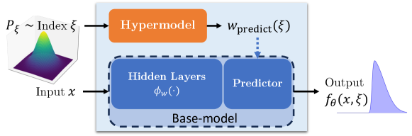
Figure 5: Description of the hypermodel: we made an assumption that the injected randomness only from the linear layer is sufficient for posterior approximation estimation of neural network based functions.

First, we develop a hypermodel for efficient approximate the posterior over the action-value function under neural network function approximation. As illustrated in Figure 5, we made assumptions that (1) Base-model: the action-value function is linear in the feature space even when the feature is unknown and needs to be learned through the training of neural network hidden layers; and (2) Last-layer linear hypermodel: the degree of uncertainty for base-model can be represented by a linear hypermodel transforming the index distribution to the approximation posterior distribution over the last-layer; and can be used for efficient deep exploration.

The (1) base-model assumption is common in supervised learning and deep reinforcement learning, e.g. DDQN(Mnih et al., 2015; Van Hasselt et al., 2016), BBF(Schwarzer et al., 2023).

As the explanation of the (2) last-layer linear hypermodel assumption: for example, in Figure 5, suppose the hidden layers in neural networks forms the nonlinear feature mapping $\phi_{w}(\cdot)$ with parameters $w$. Our last-layer linear hypermodel assumption is formulated in Section C.3.1, with trainable $\theta=\{{\bm{A}},b,w\}$ and fixed parameters $\{{\bm{A}}_{0},b_{0},w_{0}\}$, taking the random index $\xi\in\mathbb{R}^{M}$ from reference distribution $P_{\xi}$ as input and outputs the weights for last-layer.

$$f_{\theta}(x,\xi) =\underbrace{\langle{\bm{A}}\xi+b,\phi_{w}(x)\rangle}_{\textbf{Learnable~{}}f^{L}_{\theta}(x,\xi)}+\underbrace{\langle{\bm{A}}_{0}\xi+b_{0},\phi_{w_{0}}(x)\rangle}_{\textbf{Fixed prior~{}}f^{P}(x,\xi)}$$

$$=\underbrace{\langle{\bm{A}}\xi,\phi_{w}(x)\rangle}_{\sigma_{\theta}^{L}(x,\xi)}+\underbrace{\langle{\bm{A}}_{0}\xi,\phi_{w_{0}}(x)\rangle}_{\sigma^{P}(x,\xi)}+\underbrace{\langle b,\phi_{w}(x)\rangle}_{\mu_{\theta}^{L}(x)}+\underbrace{\langle b_{0},\phi_{w}(x)\rangle}_{\mu^{P}(x)}.$$ (10)

It’s worth to note that our hypermodel only outputs the weights but not bias for last-layer.

(2) As shown in Lemma 5.1, we validate that the linear hypermodel with incremental update can approximate the posterior of action-value function in the sequential decision processes. We conjecture that last layer linear hypermodel assumption is reasonable under neural network function approximation. Through our formulation in Section C.3.1, HyperAgent is supposed to accurately estimate the learnable mean $\mu_{\theta}^{L}(x)$, which relies solely on the original input $x$, and the variation prediction $\sigma^{L}_{\theta}(x,\xi)$, which is dependent on both the original input $x$ and random index $\xi$. Since not being influenced by other components that may only depend on the random index $\xi$ like HyperDQN (Li et al., 2022a), we conjecture our last-layer linear hypermodel assumption in Section C.3.1 allows the hypermodel to capture uncertainty better. Another benefit last-layer linear hypermodel is that this structure will not result in much parameters and provide better expectation estimate.

The fixed prior model also offers prior bias and prior variation through the functions $\mu^{P}(x)$ and $\sigma^{P}(x,\xi)$. This prior function is NOT trainable so that it will not bring much computation, and designed to provide better exploration in the early stage of training. We use Xavier normal initialization for the entire network except for the prior model. For the initialization of prior model, we follow the method described in (Li et al., 2022a; Dwaracherla et al., 2020). In this way, each row of prior function is sampled from the unit hypersphere, which guarantees that the output of prior function can follow a desired Gaussian distribution.

In the context of reinforcement learning, we define the action-value function with hypermodel and DNN approximation as following. For each action $a\in\mathcal{A}$, there is a set of trainable parameters $\{{\mathbf{A}}^{a},b^{a}\}$ and fixed parameters $\{{\mathbf{A}}_{0}^{a},b_{0}^{a}\}$, i.e., the trainable set of parameters $\theta=\{w,({\mathbf{A}}^{a},b^{a}):a\in\mathcal{A}\}$ and the fixed one $\{w_{0},({\mathbf{A}}_{0}^{a},b_{0}^{a}):a\in\mathcal{A}\}$ with action-value function

$$f_{\theta}(s,a,\xi)=\underbrace{\langle{\bm{A}}^{a}\xi+b^{a},\phi_{w}(s)\rangle}_{\textbf{Learnable~{}}f^{L}_{\theta}(s,a,\xi)}+\underbrace{\langle{\bm{A}}^{a}_{0}\xi+b^{a}_{0},\phi_{w_{0}}(s)\rangle}_{\textbf{Fixed prior~{}}f^{P}(s,a,\xi)}.$$

The last-layer linear hypermodel assumption is further supported by the empirical results Figures 2 and 3 where hypermodel with incremental updates enables efficient deep exploration in RL.

C.3.2 Difference compared to prior works

Several related work can be included in the hypermodel framework introduced in Section 2.2. We will discuss the structural and algorithmic differences under the unified framework in this sections. Furthermore, we performs ablation studies concerning these mentioned differences in Section E.3.

Difference with HyperModel (Dwaracherla et al., 2020).

HyperModel (Dwaracherla et al., 2020) employs hypermodel to represent epistemic uncertainty and facilitate exploration in bandit problem. However, implementing hypermodel across entire based-model results in a significant number of parameters and optimization challenges. As a reuslts, applying HyperModel to tackle large-scale problems, like Atari games, can prove to be exceedingly difficult, as highlighted in Li et al. (2022a). Additionally, HyperModel also encounters challenges in addressing the DeepSea problem due to its substantial state space, even when the size is relatively small, as demonstrated in Section E.3. In contrast, HyperAgent offers the advantage of computation efficiency as it only applies hypermodel to the last output layer of base-model, which maintains constant parameters when scaling up the problem. HyperAgent aslo demonstrates superior data efficiency compared to HyperModel, as evidenced in Figure 13.

Structural difference with Ensemble+ (Osband et al., 2018; 2019b).

Ensemble+ applies the bootstrapped ensemble method to the entire based-model, which maintains an ensemble of $M$ value networks $\{Q_{i}(s,a),i=1,\ldots,M\}$. When combined with prior network, it has demonstrated effective exploration in chain environments with large sizes. Nevertheless, to achieve effective exploration, Ensemble+ demands a relatively large ensemble size $M$ Osband et al. (2018), which raises challenges analogous to those faced by the HyperModel. This involves managing numerous parameters and optimization issues. We also evaluated Ensemble+ with a larger $M=16$, and it still proved ineffective in solving the DeepSea, as depicted in Figure LABEL:fig:deepsea_ois, highlighting the superior data efficiency of HyperAgent.

Structural difference with hypermodel in HyperDQN (Li et al., 2022a).

HyperDQN shares a similar structure with HyperAgent and has demonstrated promising results in exploration. Nevertheless, it struggles to handle the DeepSea, which requires deep exploration, as depicted in Figure 2. We enhanced HyperDQN by simplifying the hypermodel, as demonstrated in Section C.3.1. HyperAgent estimates the mean $\mu$ exclusively from the original input $x$ and estimates the variation $\sigma$ using both the original input $x$ and the random index ${\bm{\xi}}$. In the implementation of HyperDQN, there are two linear hypermodel $f_{\theta_{1}}(\xi)$ and $f_{\theta_{2}}(\xi)$.

$$f_{\theta_{1}}(\xi) ={\bm{A}}_{1}\xi+b_{1}; f_{\theta_{2}}(\xi) ={\bm{A}}_{2}\xi+b_{2}.$$

$$f_{\theta_{1}^{P}}(\xi) ={\bm{A}}^{P}_{1}\xi+b^{P}_{1}; f_{\theta_{2}^{P}}(\xi) ={\bm{A}}^{P}_{2}\xi+b^{P}_{2}.$$

The hypermodel $f_{\theta_{1}}(\xi)$ outputs weights for last output layer of base-model, and hypermodel $f_{\theta_{2}}(\xi)$ outputs bias for last output layer of base-model. The functions $f_{\theta^{P}_{1}}(\xi)$ and $f_{\theta^{P}_{2}}(\xi)$ are the prior network corresponding to trainable linear hypermodel. These linear hypermodel contain trainable $\theta_{1}=\{{\bm{A}}_{1},b_{1}\}$, $\theta_{2}=\{{\bm{A}}_{2},b_{2}\}$ and fixed parameters $\theta^{P}_{1}=\{{\bm{A}}^{P}_{1},b^{P}_{1}\}$, $\theta^{P}_{2}=\{{\bm{A}}^{P}_{2},b^{P}_{2}\}$. Therefore, the implementation of HyperDQN can be formulated by

$$f^{\operatorname{HyperDQN}}(x,\xi) =\langle f_{\theta_{1}}(\xi),\phi_{w}(x)\rangle+f_{\theta_{2}}(\xi)+\langle f_{\theta_{1}^{P}}(\xi),\phi^{P}_{w}(x)\rangle+f_{\theta^{P}_{2}}(\xi)$$

$$=\underbrace{\langle b_{1},\phi_{w}(x)\rangle}_{\mu^{L}(x)}+\underbrace{\langle{b^{P}_{1}},\phi^{P}_{w}(x)\rangle}_{\mu^{P}(x)}+\underbrace{\langle{\bm{A}}_{1}\xi,\phi_{w}(x)\rangle}_{\sigma_{1}^{L}(,\xi)}+\underbrace{\langle{{\bm{A}}^{P}_{1}}\xi,\phi^{P}_{w}(x)\rangle}_{\sigma_{1}^{P}(,\xi)}+$$

$$\quad\quad\underbrace{{\bm{A}}_{2}\xi}_{\sigma_{2}^{L}(\xi)}+\underbrace{{\bm{A}}^{P}_{2}\xi}_{\sigma_{2}^{P}(\xi)}+\underbrace{{b_{2}}}_{\mu^{L}_{3}}+\underbrace{{b^{P}_{2}}}_{\mu^{P}_{3}}.$$ (11)

As demonstrated in Equation 11, HyperDQN utilizes the hypermodel to generate both weights and bias for the output layer, leading to redundant components, such as functions ($\sigma_{2}^{L}(\xi)$, $\sigma_{2}^{P}(\xi)$) that rely solely on the random index ${\bm{\xi}}$, or functions ($\mu^{L}_{3}$, $\mu^{P}_{3}$) that do not depend on any inputs. These components lack a clear semantic explanation. We also found that initializing the hypermodel with Xavier Normal can improve optimization. These modifications are some of the factors leading to HyperAgent outperforming HyperDQN on both DeepSea and Atari games, as demonstrated in Section 4.

Structural difference with epinet in ENNDQN (Osband et al., 2023a; b).

ENNDQN Osband et al. (2023b), leveraging the epinet Osband et al. (2023a) structure, exhibits potential in capturing epistemic uncertainty and has showcased effectiveness across diverse tasks. In the network structure of epinet, the original input $x$, feature $\phi_{w}(x)$, and random index ${\bm{\xi}}$ are concatenated as the input for the last output layer. An ensemble prior function with size $M$ is used for the output layer, but a prior function for the feature network is not present. This network structure results in larger parameters when handling tasks at a large scale, creating notable computation and optimization challenges. For instance, in the case of DeepSea with a size of 20, the parameters of epinet are nearly 20 times larger than those of HyperAgent. This is due to the raw state input $x\in\mathbb{R}^{N^{2}}$ for DeepSea with size $N$, whose dimension $N^{2}$ is too large for the epinet to effectively process. As as results, epinet struggles with larger scale of the problem, as evidenced in Figure 13. In contrast, HyperAgent takes only a random index ${\bm{\xi}}$ and feature $\phi_{w}(x)$ as input for output layer, resulting in more efficient computation with fewer constant parameters.

Algorithmic difference with Ensemble+, HyperDQN and ENNDQN.

For a transition tuple $d=(s,a,r,s^{\prime},{\mathbf{z}})\in D$ and given a single index $\xi$, with main hypermodel parameters $\theta$ and target hypermodel parameters $\theta^{-}$, the loss in these works can be represented using our notion of hypermodel:

• The temporal difference (TD) loss for Ensemble+ (Osband et al., 2018; 2019b) inherits the BootDQN (Osband et al., 2016),

  $$\ell^{\gamma}_{\operatorname{Ensemble+}}(\theta;\theta^{-},\xi,d) =({\mathbf{z}}^{\top}\xi)\left(f^{\operatorname{Ensemble+}}_{\theta}(s,a,\xi)-(r+\gamma\max_{a^{\prime}\in\mathcal{A}}f^{\operatorname{Ensemble+}}_{\theta^{-}}(s^{\prime},a^{\prime},\xi))\right)^{2},$$ (12)

  where $f^{\operatorname{Ensemble+}}$ is the ensemble network structure, $\xi\sim P_{\xi}:=\mathcal{U}(\{e_{1},\ldots,e_{M}\})$ where $e_{i}$ is the one-hot vector in $\mathbb{R}^{M}$ and ${\mathbf{z}}\sim P_{{\mathbf{z}}}$, where ${\mathbf{z}}_{i}$ sampled from $2\cdot\operatorname{Bernoulli}(0.5)$ independently across entries $i\in[M]$.

• The TD loss for HyperDQN (Li et al., 2022a) is

  $$\ell^{\gamma,\sigma}_{\operatorname{HyperDQN}}(\theta;\theta^{-},\xi,d) =\left(f^{\operatorname{HyperDQN}}_{\theta}(s,a,\xi)-(r+\sigma{\mathbf{z}}^{\top}\xi\gamma+\max_{a^{\prime}\in\mathcal{A}}f^{\operatorname{HyperDQN}}_{\theta^{-}}(s^{\prime},a^{\prime},\xi))\right)^{2},$$ (13)

  where $f^{\operatorname{HyperDQN}}$ is the network structure of HyperDQN, $\xi\sim P_{\xi}:=\mathcal{U}(\mathbb{S}^{M-1})$ and ${\mathbf{z}}\sim P_{{\mathbf{z}}}:=\mathcal{U}(\mathbb{S}^{M-1})$.

• The TD loss for ENNDQN (Osband et al., 2023b) is

  $$\ell^{\gamma}_{\operatorname{ENNDQN}}(\theta;\theta^{-},\xi,d) =\left(f^{\operatorname{epinet}}_{\theta}(s,a,\xi)-(r+\gamma\max_{a^{\prime}\in\mathcal{A}}f^{\operatorname{epinet}}_{\theta^{-}}(s^{\prime},a^{\prime},\xi))\right)^{2},$$ (14)

  where $f^{\operatorname{epinet}}$ is the epinet structure used in ENNDQN, $\xi\sim P_{\xi}:=N(0,I_{M})$.

As discussed in this section, $f^{\operatorname{Ensemble+}},f^{\operatorname{HyperDQN}},f^{\operatorname{epinet}}$ can all be represented within our hypermodel framework and our construction of hypermodel in HyperAgent has a few mentioned advantages. The key difference in these loss functions Equations 12, 13 and 14 is that the index $\xi$ used for target computation is the same one as in main network; while in Equation 2 of HyperAgent, we choose a target index mapping ${\bm{\xi}}^{-}$ that is independent of $\xi$. Our choice is critical for theoretical analysis as closed-form solution under linear or tabular representation can be derived with Equation 2 of HyperAgent but can NOT be derived with Equations 12, 13 and 14 of any previous related works. The empirical difference for this issue will be discussed in ablation studies in Section E.3. Another issue is that whether we need a additive perturbation. As stated in the incremental update Equation 5, the std of artificial perturbation $\sigma$ is important for our posterior approximation argument Lemma 5.1. However, in some practical problems with deterministic transitions, do we really need this level of perturbations i.e., $\sigma=0$ or $\sigma>0$? If we need $\sigma>0$, how large should it be? This issue would be address in Section E.2.

C.4 Tabular representations

To understand and analyze the behavior of HyperAgent, we specify the algorithm in the tabular setups. Notice that the closed-form iterative update rule derived here is general and can be applied for infinite-horizon and finite horizon problems.

Hypermodel in HyperAgent with tabular representation would be

$$f_{\theta}(s,a,\xi)=\underbrace{\mu_{sa}+m_{sa}^{\top}\xi}_{\textbf{Learnable model}~{}f^{L}_{\theta}(s,a,\xi)}+\underbrace{\mu_{0,sa}+\sigma_{0}{\mathbf{z}}_{0,sa}^{\top}\xi}_{\textbf{Prior model}~{}f^{P}(s,a,\xi)}$$

where $\theta=(\mu\in\mathbb{R}^{|\mathcal{S}||\mathcal{A}|},m\in\mathbb{R}^{|\mathcal{S}||\mathcal{A}|\times M})$ are the parameters to be learned, and ${\mathbf{z}}_{0,sa}\in\mathbb{R}^{M}$ is a independent random vector sampled from $P_{{\mathbf{z}}}$ and $\mu_{0,sa},\sigma_{0}$ is a prior mean and prior variance for each $(s,a)\in\mathcal{S}\times\mathcal{A}$. The tabular representation is related to the last-layer linear hypermodel assumption in Section C.3.1 when the hidden layer maps $(s,a)$ to a fixed one-hot feature $\phi_{w}(s,a)=\mathds{1}_{sa}$ and $d=|\mathcal{S}||\mathcal{A}|$. The regularizer in Equation 3 then becomes $\beta\|\theta\|^{2}=\beta\sum_{s,a}\left(\mu_{sa}^{2}+\|m_{sa}\|^{2}\right)$.

Derivations of Equations 5, 6 and 7 in Section 5.

The derivation is mainly from the separability of optimization problem in tabular setup. Let $\theta_{sa}=(\mu_{sa},m_{sa})$ be the optimization variable for specific $(s,a)\in\mathcal{S}\times\mathcal{A}$. As mentioned in Section 5, at the beginning of episode $k$, with $D=\mathcal{H}_{k}$ and target noise mapping ${\bm{\xi}}^{-}={\bm{\xi}}_{k}$, we iterative solve Equation 3 by taking target parameters $\theta^{-}=\theta^{(i)}_{k}$ as previous solved iterate starting from $\theta^{(0)}_{k}=\theta_{k-1}=(\mu_{k-1},m_{k-1})$ as the solution for previous episode $k-1$.

Let the optimal solution in $(i)$-th iteration be $\theta^{(i+1)}_{k}=\operatorname*{arg\,min}_{\theta}{L}^{\gamma,\sigma,\beta}(\theta;\theta^{-}=\theta^{(i)}_{k},{\bm{\xi}}^{-}={\bm{\xi}}_{k},\mathcal{H}_{k})$. In tabular setting, by the separability of the objective function in Equation 3, we have $\theta_{k,sa}=(\mu_{k,sa},m_{k,sa})=\operatorname*{arg\,min}_{\theta_{sa}}L_{sa}(\theta_{sa};\theta^{-}=\theta^{(i)}_{k},{\bm{\xi}}^{-}={\bm{\xi}}_{k},\mathcal{H}_{k}))$ where $\operatorname*{arg\,min}_{\theta_{sa}}L_{sa}(\theta_{sa};\theta^{-},{\bm{\xi}}^{-},\mathcal{H}_{k})$ is defined as

$$\operatorname*{arg\,min}_{\theta_{sa}} \mathbb{E}_{\xi\sim P_{\xi}}[\sum_{\ell=1}^{k-1}\sum_{t\in E_{\ell,sa}}(f_{\theta}(S_{\ell,t},A_{\ell,t},\xi)-(\sigma\xi^{\top}{\mathbf{z}}_{\ell,t+1}+y_{\ell,t+1}(\theta^{-},{\bm{\xi}}^{-})))^{2}]+{\beta}(\mu_{sa}^{2}+\|m_{sa}\|^{2})$$

$$=\operatorname*{arg\,min}_{\theta_{sa}} \mathbb{E}_{\xi\sim P_{\xi}}[\sum_{\ell=1}^{k-1}\sum_{t\in E_{\ell,sa}}(f_{\theta}(s,a,\xi)-(\sigma\xi^{\top}{\mathbf{z}}_{\ell,t+1}+y_{\ell,t+1}(\theta^{-},{\bm{\xi}}^{-})))^{2}]+{\beta}(\mu_{sa}^{2}+\|m_{sa}\|^{2})$$

$$=\operatorname*{arg\,min}_{(\mu_{sa},m_{sa})} \mathbb{E}_{\xi\sim P_{\xi}}[\sum_{\ell=1}^{k-1}\sum_{t\in E_{\ell,sa}}((\mu_{sa}+\mu_{0,sa})+(m_{sa}+\sigma_{0}{\mathbf{z}}_{0,sa})^{\top}\xi-(\sigma\xi^{\top}{\mathbf{z}}_{\ell,t+1}+y_{\ell,t+1}(\theta^{-},{\bm{\xi}}^{-})))^{2}]$$

$$\quad\quad+{\beta}(\mu_{sa}^{2}+\|m_{sa}\|^{2})$$

where the target value is

$$y_{\ell,t+1}(\theta^{-},{\bm{\xi}}^{-})=R_{\ell,t+1}+\gamma\max_{a^{\prime}\in\mathcal{A}}f_{\theta^{-}}(S_{\ell,t+1},a^{\prime},{\bm{\xi}}^{-}(S_{\ell,t+1})).$$

With some calculations, the closed form solution of $\theta^{(i+1)}_{k}=(\mu_{k,sa}^{(i+1)},m_{k,sa})$ is

$$m_{k,sa}+\sigma_{0}{\mathbf{z}}_{0,sa} =\frac{\sigma\sum_{\ell=1}^{k-1}\sum_{t\in E_{\ell,sa}}{\mathbf{z}}_{\ell,t+1}+\beta\sigma_{0}{\mathbf{z}}_{0,sa}}{N_{k,sa}+\beta}$$

$$=\frac{(N_{k-1,sa}+\beta)(m_{k-1,sa}+\sigma_{0}{\mathbf{z}}_{0,sa})+\sigma\sum_{t\in E_{k-1,sa}}{\mathbf{z}}_{\ell,t+1}}{N_{k,sa}+\beta},$$

which derives the incremental update in Equation 5, and

$$\mu_{k,sa}^{(i+1)}=\frac{\sum_{\ell=1}^{k-1}\sum_{t\in E_{\ell,sa}}y_{\ell,t+1}(\theta^{-}=\theta_{k}^{(i)},{\bm{\xi}}^{-}={\bm{\xi}}_{k})+\beta\mu_{0,sa}}{N_{k,sa}+\beta}.$$ (15)

Recall some short notations: (1) $V_{Q}$ is greedy value with respect to $Q$ such that $V_{Q}(s)=\max_{a\in\mathcal{A}}Q(s,a)$ for all $s\in\mathcal{S}$; (2) $f_{\theta,{\bm{\xi}}}(s,a)=f_{\theta}(s,a,{\bm{\xi}}(s)),\forall(s,a)\in\mathcal{S}\times\mathcal{A}$. Recall the stochastic bellman operator $F_{k}^{\gamma}$ induced by HyperAgent,

$$F_{k}^{\gamma}Q(s,a) :=\frac{\beta\mu_{0,sa}+N_{k,sa}(r_{sa}+\gamma V_{Q}^{\top}\hat{P}_{k,sa})}{N_{k,sa}+\beta}+m_{k,sa}^{\top}{\bm{\xi}}_{k}(s),\quad\forall(s,a)\in\mathcal{S}\times\mathcal{A}.$$

With the following observation,

$$\sum_{\ell=1}^{k-1}\sum_{t\in E_{\ell,sa}}y_{\ell,t+1}(\theta^{-},{\bm{\xi}}^{-}) =N_{k,sa}(r_{sa}+\gamma\sum_{s^{\prime}\in\mathcal{S}}\hat{P}_{k,sa}(s^{\prime})(\max_{a^{\prime}\in\mathcal{A}}f_{\theta^{-}}(s^{\prime},a^{\prime},{\bm{\xi}}^{-}(s^{\prime})))),$$

from Equation 15, we have for all pairs $(s,a)$

$$f_{\theta_{k}^{(i+1)}}(s,a,{\bm{\xi}}_{k}) =\mu_{k,sa}^{(i+1)}+m_{k,sa}^{\top}{\bm{\xi}}_{k}(s)=\frac{\beta\mu_{0,sa}+N_{k,sa}(r_{sa}+\gamma V_{f_{\theta_{k}^{(i)},{\bm{\xi}}_{k}}}^{\top}\hat{P}_{k,sa})}{N_{k,sa}+\beta}+m_{k,sa}^{\top}{\bm{\xi}}_{k}(s),$$

which is essentially bellman iteration under stochastic bellman operator induced by HyperAgent,

$$f_{\theta_{k}^{(i+1)},{\bm{\xi}}_{k}}=F^{\gamma}_{k}f_{\theta_{k}^{(i)},{\bm{\xi}}_{k}}.$$

Lemma C.1 (Contraction mapping).

Let $B(\mathcal{S}\times\mathcal{A})$ be the space of bounded functions $Q:\mathcal{S}\times\mathcal{A}\rightarrow\mathbb{R}$. Let $\rho$ be the distance metric $\rho(Q,Q^{\prime})=\sup_{(s,a)\in\mathcal{S}\times\mathcal{A}}|Q(s,a)-Q^{\prime}(s,a)|$. For all $k\in\mathbb{Z}_{++}$ the Bellman operator of HyperAgent $F^{\gamma}_{k}:B(\mathcal{S}\times\mathcal{A})\rightarrow B(\mathcal{S}\times\mathcal{A})$ is a contraction mapping with modulus $\gamma\in[0,1)$ in metric space $(B(\mathcal{S}\times\mathcal{A}),\rho)$.

By Lemma C.1, since contraction mapping, the bellman operator of HyperAgent $F^{\gamma}_{k}$ has a unique fixed point and the iterative process in Equation 6 can converge to a unique fixed point $\theta_{k}$. Essentially, due the algorithmic randomness introduced in the iterative process, $f_{\theta_{k},{\bm{\xi}}_{k}}$ is a randomized state-action value function.

Proof of Lemma C.1.

By Blackwell’s sufficient conditions, we need to show that $F^{\gamma}_{k}$ satisfies the following two conditions:

1. Monotonicity: for all $Q,Q^{\prime}\in B(\mathcal{S}\times\mathcal{A})$, if $Q(s,a)\leq Q^{\prime}(s,a)$ for all $(s,a)\in\mathcal{S}\times\mathcal{A}$, then

$$F_{k}^{\gamma}Q(s,a)\leq F_{k}^{\gamma}Q^{\prime}(s,a)$$

2. Discounting: for all $(s,a)\in\mathcal{S}\times\mathcal{A}$, all $c\geq 0$ and $Q\in B(\mathcal{S}\times\mathcal{A})$,

$$[F^{\gamma}_{k}(Q+c)](s,a)-[F^{\gamma}_{k}Q](s,a)=\left(\frac{N_{k,sa}}{N_{k,sa}+\beta}\right)\gamma c\leq\gamma c$$

∎

True Bellman Operator.

For any MDP ${\mathcal{M}}=(\mathcal{S},\mathcal{A},r,P,\rho,s_{\operatorname{terminal}})$, consider a function $Q\in B(\mathcal{S}\times\mathcal{A})$. The true Bellman operator, when applied to $Q$, is defined as follows:

$$F_{{\mathcal{M}}}^{\gamma}Q(s,a) =r_{sa}+\gamma V_{Q}^{\top}P_{sa},\quad\forall(s,a)\in\mathcal{S}\times\mathcal{A}.$$ (16)

As will be introduced later, under Dirichlet prior Assumption D.9, given the randomness in $P$, $F_{{\mathcal{M}}}^{\gamma}$ is essentially stochastic in nature. When $F_{{\mathcal{M}}}^{\gamma}$ acts upon a state-action value function $Q\in B(\mathcal{S}\times\mathcal{A})$, the result is a randomized state-action value function.

Appendix D Insight and Theoretical analysis of HyperAgent

D.1 Sequential posterior approximation argument in Lemma 5.1

We use short notation for $[n]=\{1,2,\ldots,n\}$ and $\mathcal{T}=\{0,1,\ldots,T\}=\{0\}\cup[T]$. Before digging into the details of proof of our key lemma, let us first introduce some useful probability tools developed for random projection recently.

Lemma D.1 (Distributional JL lemma (Johnson & Lindenstrauss, 1984)).

For any $0<\varepsilon,\delta<1/2$ and $d\geq 1$ there exists a distribution $\mathcal{D}_{\varepsilon,\delta}$ on $\mathbb{R}^{M\times d}$ for $M=O\left(\varepsilon^{-2}\log(1/\delta)\right)$ such that for any ${\bm{x}}\in\mathbb{R}^{d}$

$$\underset{\Pi\sim\mathcal{D}_{\varepsilon,\delta}}{\mathbb{P}}\left(\|\Pi{\bm{x}}\|_{2}^{2}\notin\left[(1-\varepsilon)\|{\bm{x}}\|_{2}^{2},(1+\varepsilon)\|{\bm{x}}\|_{2}^{2}\right]\right)<\delta$$

Theorem D.2 (Unified analysis of random projection (Li, 2024b)).

We claim that the following construction of the random projection matrix $\Pi\in\mathbb{R}^{M\times d}$ with $M\geq 64\varepsilon^{-2}\log(2/\delta)$ satisfy the distributional JL lemma in Lemma D.1: Let $\Pi=({\mathbf{z}}_{1},\ldots,{\mathbf{z}}_{d})$ be a random matrix with each ${\mathbf{z}}_{i}\sim P_{{\mathbf{z}}}$ where $P_{{\mathbf{z}}}$ can be any $\frac{1}{\sqrt{M}}$-sub-Gaussian distribution over $\mathbb{R}^{M}$ with unit-norm, e.g., uniform distribution over the unit sphere $\mathcal{U}(\mathbb{S}^{M-1})$.

Remark D.3.

As discussed in (Li, 2024b), all previous analysis for random projection can NOT handle spherical construction of the random projection matrix where ${\mathbf{z}}_{i}$ sampled from $\mathcal{U}(\mathbb{S}^{M-1})$. This is because all analysis in literature requires independence across the entries of ${\mathbf{z}}_{i}$. Therefore, Theorem D.2 is important for our analysis in Lemma 5.1 as our perturbation random vector is from $\mathcal{U}(\mathbb{S}^{M-1})$.

Theorem D.4 (Sequential random projection in adaptive process (Li, 2024a)).

Let $(\mathcal{F}_{t})_{t\geq 0}$ be a filtration. For any fixed $\varepsilon\in(0,1)$ any fixed $s\in\mathbb{R}_{+}$, let ${\mathbf{s}}\in\mathbb{R}^{M}$ be an $\mathcal{F}_{0}$-measurable random vector satisfies $\mathbb{E}[\|{\mathbf{s}}\|^{2}]=s^{2}$ and $|\|{\mathbf{s}}\|^{2}-s^{2}|\leq(\varepsilon/2)s^{2}$. Let $({\mathbf{z}}_{t})_{t\geq 1}\subset\mathbb{R}^{M}$ be a stochastic process adapted to filtration $(\mathcal{F}_{t})_{t\geq 1}$ such that it is $\sqrt{c_{0}/M}$-sub-Gaussian and each ${\mathbf{z}}_{t}$ is unit-norm. Let $(x_{t})_{t\geq 1}\subset\mathbb{R}$ be a stochastic process adapted to filtration $(\mathcal{F}_{t-1})_{t\geq 1}$ such that it is $c_{x}$-bounded. Here, $c_{0}$ and $c_{x}$ are absolute constants. If the following condition is satisfied

$$M\geq\frac{16c_{0}(1+\varepsilon)}{\varepsilon^{2}}\left(\log\left(\frac{1}{\delta}\right)+\log\left(1+\frac{c_{x}T}{s^{2}}\right)\right),$$

we have, with probability at least $1-\delta$

$$\forall t\in\mathcal{T},\quad(1-\varepsilon)\left(s^{2}+\sum_{i=1}^{t}x_{i}^{2}\right)\leq\|{\mathbf{s}}+\sum_{i=1}^{t}x_{i}{\mathbf{z}}_{i}\|^{2}\leq(1+\varepsilon)\left(s^{2}+\sum_{i=1}^{t}x_{i}^{2}\right).$$

Remark D.5.

Li (2024a) claims this is an “sequential random projection” argument because one can relate Theorem D.4 to the traditional random projection setting where $\Pi=({\mathbf{z}}_{1},\ldots,{\mathbf{z}}_{T})\in\mathbb{R}^{M\times T}$ is a random projection matrix and ${\bm{x}}=(x_{1},\ldots,x_{T})^{\top}\in\mathbb{R}^{T}$ is the vector to be projected. When $s=0$ and ${\mathbf{s}}=0$, this is essentially an analog of distributional JL lemma (described in Lemma D.1) while all previous analytical techniques including Theorem D.2 for JL lemma are NOT able to handle the sequential dependence structure in this sequential setup. This is due to the fact that they require the vector ${\bm{x}}$ to be a fixed vector in their analysis. Due to the dependence issue between ${\bm{x}}$ and $\Pi$, when conditioned on ${\bm{x}}$, the distribution of $\Pi$ changed and all technical tools in literature fails to handle this situation.

Proof of Lemma 5.1.

Step 1: Prior approximation. We first show the prior approximation by the fixed prior model, i.e. the event $\mathcal{G}_{0,sa}(\varepsilon/2)=\{|\|\sigma_{0}{\mathbf{z}}_{0,sa}\|^{2}-\sigma_{0}^{2}|\leq\frac{\varepsilon}{2}\sigma_{0}^{2}\}$ holds for any $(s,a)$, using the unified analysis (Theorem D.2) for spherical construction of the random projection matrix. With Theorem D.2, we can show that if $M\geq 256\varepsilon^{-2}\log(4|\mathcal{S}||\mathcal{A}|/\delta)$, $\cap_{(s,a)\in\mathcal{S}\times\mathcal{A}}\mathcal{G}_{0,sa}$ holds with probability at least $1-\delta/2$ by union bound.

Step 2: Posterior approximation. Recall that $\beta=\sigma^{2}/\sigma_{0}^{2}$. To handle the posterior approximation, we define a sequence of indicator variables

$$x_{\ell,t}=\mathds{1}_{t\in E_{\ell,sa}},$$

where $E_{\ell,sa}$ is the collection of time steps in episode $\ell$ encountering state-action pair $(s,a)$. We also define auxiliary notations ${\mathbf{s}}=\sqrt{\beta}{\mathbf{z}}_{0,sa}$ and $s=\sqrt{\beta}$. Then, Equation 5 now becomes

$$\frac{(N_{k,sa}+\beta)}{\sigma}m_{k,sa} =\sqrt{\beta}{\mathbf{z}}_{0,sa}+\sum_{\ell=1}^{k-1}\sum_{t\in E_{\ell}}x_{\ell,t}{\mathbf{z}}_{\ell,t+1}$$ (17)

Importantly, the sequential dependence structure in HyperAgent when interacting with environment is that

• $x_{\ell,t}$ dependents on the environmental and algorithmic randomness in all previous time steps:

  $${\mathbf{s}},(x_{1,t^{\prime}},{\mathbf{z}}_{1,t^{\prime}+1})_{t^{\prime}\in E_{1}},(x_{2,t^{\prime}},{\mathbf{z}}_{2,t^{\prime}+1})_{t^{\prime}\in E_{2}},\ldots,(x_{\ell,t^{\prime}},{\mathbf{z}}_{\ell,t^{\prime}+1})_{t^{\prime}<t};$$

• and ${\mathbf{z}}_{\ell,t+1}$ is independent of the environmental and algorithmic randomness in all previous time steps:

  $${\mathbf{s}},(x_{1,t^{\prime}},{\mathbf{z}}_{1,t^{\prime}+1})_{t^{\prime}\in E_{1}},(x_{2,t^{\prime}},{\mathbf{z}}_{2,t^{\prime}+1})_{t^{\prime}\in E_{2}}\ldots,(x_{\ell,t^{\prime}+1},{\mathbf{z}}_{\ell,t^{\prime}+1})_{t^{\prime}<t},x_{\ell,t},$$

where $E_{\ell}$ is the collection of times steps in episode $\ell$. The difficulty of posterior approximation comes from the above dependence structure as we can not directly use argument conditioning on the entire history $\mathcal{H}_{\ell}$ at once. This is because the conditional distributions of $({\mathbf{z}}_{\ell^{\prime},t^{\prime}})$ given $\mathcal{H}_{\ell}$ are changed from the unconditional one. Besides, the random variables $(({\mathbf{z}}_{\ell^{\prime},t^{\prime}})$ are not conditionally independent given $\mathcal{H}_{\ell}$. This difficulty calls for the innovation on fundamental tools in probability with martingale analysis, as shown in Theorem D.4.

Prior approximation guarantees the initial condition $|\|s\|^{2}-s^{2}|\leq({\varepsilon}/{2})s^{2}$ in Theorem D.4. We observe that for all $(k,s,a)$, $x_{k,sa}\leq 1$ and $\sum_{\ell=1}^{k-1}x_{k,sa}^{2}=N_{k,sa}$. Also, as proved in (Li, 2024b; a), at each time step $(\ell,t)$, the perturbation random vector ${\mathbf{z}}_{\ell,t}\sim P_{{\mathbf{z}}}:=\mathcal{U}(\mathbb{S}^{M-1})$ is the $\frac{1}{\sqrt{M}}$-sub-Gaussian random variable in $\mathbb{R}^{M}$.

We now can apply Theorem D.4 to the RHS of Equation 17 with sequence $({\mathbf{z}}_{\ell,t})$ and $(x_{\ell,t})$ yields the results $\mathbb{P}(\cap_{k=1}^{K+1}\mathcal{G}_{k,sa}(\varepsilon))\geq 1-\delta/2$ if

$$M\geq\frac{16(1+\varepsilon)}{\varepsilon^{2}}\left(\log\left(\frac{2}{\delta}\right)+\log\left(1+\frac{T}{\beta}\right)\right),$$

where $\sum_{k=1}^{K}|E_{k}|=T$ almost surely. Then by union bound over the set $\mathcal{S}\times\mathcal{A}$ yields the results: if

$$M\geq\max\left\{\frac{256}{\varepsilon^{2}}\log\left(\frac{4|\mathcal{S}||\mathcal{A}|}{\delta}\right),\frac{16(1+\varepsilon)}{\varepsilon^{2}}\left(\log\left(\frac{2|\mathcal{S}||\mathcal{A}|}{\delta}\right)+\log\left(1+\frac{T}{\beta}\right)\right)\right\},$$ (18)

we have $\mathbb{P}\left(\cap_{(s,a)\in\mathcal{S}\times\mathcal{A}}\cap_{k=1}^{K+1}\mathcal{G}_{k,sa}(\varepsilon)\right)\geq 1-\delta.$ ∎

Remark D.6.

According to the proof, the above sequential posterior approximation argument Lemma 5.1 holds for any tabular MDP. It do NOT rely on any assumptions made latter for regret analysis. If the tabular MDP follows Assumption D.8, the same result in Lemma 5.1 holds when

$$M\geq M(\varepsilon):=\max\left\{\frac{256}{\varepsilon^{2}}\log\left(\frac{4|\mathcal{X}|H|\mathcal{A}|}{\delta}\right),\frac{16(1+\varepsilon)}{\varepsilon^{2}}\left(\log\left(\frac{2|\mathcal{X}|H|\mathcal{A}|}{\delta}\right)+\log\left(1+\frac{K}{\beta}\right)\right)\right\},$$ (19)

where $|\mathcal{S}|=SH$. The difference in $\log(1+K/\beta)$ term is due to the fact we apply Theorem D.4 for random variables only in a single stage $t$ across episode $\ell=1,\ldots,K$ under Assumption D.8 since the visitation counts $N_{k,(t,x),a}$ only takes the historical data in stage $t$ into considerations for all $(t,x)\in\mathcal{S}_{t}$, $a\in\mathcal{A}$ and $t\in\{0,\ldots,H-1\}$.

D.2 Insight: How does HyperAgent drives efficient deep exploration?

In this section, we highlight the key components of HyperAgent that enable efficient deep exploration. We consider a simple example (adapted from (Osband et al., 2019b)) to understand the HyperAgent’s learning rule in Equations 3 and 4 and the role of hypermodel, and how they together drive efficient deep exploration.

Example D.7.

Consider a fixed horizon MDP $\mathcal{M}$ with four states $\mathcal{S}=\{1,2,3,4\}$, two actions $\mathcal{A}=\{up,down\}$ and a horizon of $H=6$. Let us consider the scenario when the agent is at the beginning of $k$-th episode. Let $\mathcal{H}_{k}$ be the history of all transitions observed prior to episode $k$, and let $\mathcal{H}_{k,sa}=\left(\left(\hat{s},\hat{a},r,s^{\prime}\right)\in\mathcal{H}^{k}:(\hat{s},\hat{a})=(s,a)\right)$ contain the transitions from state-action pair $(s,a)$ encountered before episode $k$. Suppose $|\mathcal{H}^{k}_{4,down}|=1$, while for every other pair $(s,a)\neq(4,{down}),\left|\mathcal{D}_{s,a}\right|$ is very large, virtually infinite. Hence, we are highly certain about the expected immediate rewards and transition probabilities except for $(4,{down})$.

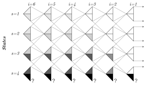
Figure 6: Example to illustrate how HyperAgent achieves deep exploration. We can see the propagation of uncertainty from later time period to earlier time period in the figure. Darker shade indicates higher degree of uncertainty.

From Equations 5, 6 and 7, HyperAgent produces a sequence of action-value functions $Q^{(i)}:=f_{\theta_{k}^{(i)}}$ for $i=0,1,2,\ldots,6$ as shown in Figure 6 by iteratively solving Equation 3 starting from $Q^{(0)}=\mathbf{0}$,

$$Q^{(i+1)}(s,a) =F^{\gamma}_{k}Q^{(i)}(s,a)=\frac{\beta\mu_{0,sa}+N_{k,sa}(r_{sa}+\gamma V_{Q^{(i)}}^{\top}\hat{P}_{k,sa})}{N_{k,sa}+\beta}+\tilde{m}_{k,sa}^{\top}{\bm{\xi}}_{k}(s),$$

In Figure 6, each triangle in row $s$ and column $t$ contains two smaller triangles that are associated with action-values of $up$ and $down$ actions at state $s$. The shade on the smaller triangle shows the uncertainty estimates in the $Q^{(i)}(s,a)$, specifically the variance. The dotted lines show plausible transitions, except at $(4,down)$. Since we are uncertain about $(4,down)$, any transition is plausible.

As shown in the Figure 6, when $i=1$, since data size at $(s,a)\neq(4,\text{down})$ tends to infinity, $\|\tilde{m}_{k,sa}\|^{2}\approx 0$ from our Lemma 5.1, thus almost zero variance and white colored at $(s,a)\neq(4,\text{down})$; while $(s,a)=(4,\text{down})$ exhibits large variance, thus dark share, due to the lack of data $|\mathcal{H}_{k,(4,\text{down})}|=1$ and Lemma 5.1. By performing bellman update, the noise term ${\tilde{m}_{k,sa}}^{\top}{\bm{\xi}}_{k}(s)$ at $(s,a)=(4,\text{down})$ is back-propagated to other states consecutively by the iterative process $i=2,3,4,5$. This is because other state-action pairs may lead to the transition into $(4$, down$)$, thus being influenced by the variance introduced by the estimation of $\mathcal{Q}^{(1)}(4$, down$)$. As traced in Figure 6, it’s clear that the propagation of noise affects the value estimates in a pattern depicted by the figure’s shading.

This dynamic is crucial for fostering deep exploration. In essence, a sample $\mathcal{Q}^{(6)}(s,a)$ with high variance may appear excessively optimistic in certain episodes, incentivizing the agent to explore that action. Such exploration is justified by the agent’s uncertainty about the true optimal value $Q^{*}(s,a)$ across the planning horizon. This incentive extends beyond just the immediate reward and transition uncertainty. As depicted in Figure 6, the spread of uncertainty through the system creates incentives for the agent to seek out information, potentially over several time steps, to make a informative observation. This process underlines the core principle of deep exploration.

D.3 Provable scalability and efficiency of HyperAgent

D.3.1 Assumptions

Assumption D.8 (Finite-horizon time-inhomogeneous MDPs).

We consider a problem class that can be formulated as a special case of the general formulation in Section 2. Assume the state space factorizes as $\mathcal{S}=\mathcal{S}_{0}\cup\mathcal{S}_{1}\cup\mathcal{S}_{2}\cup\cdots\cup\mathcal{S}_{H-1}$ where the state always advances from some state $s_{t}\in\mathcal{S}_{t}$ to $s_{t+1}\in\mathcal{S}_{t+1}$ and the process terminates with probability 1 in period $H$, i.e.,

$$\sum_{s^{\prime}\in\mathcal{S}_{t+1}}{P}_{sa}\left(s^{\prime}\right)=1\quad\forall t\in\{0,\ldots,H-2\},s\in\mathcal{S}_{t},a\in\mathcal{A}$$

and

$$\sum_{s^{\prime}\in\mathcal{S}}{P}_{sa}\left(s^{\prime}\right)=0\quad\forall s\in\mathcal{S}_{H-1},a\in\mathcal{A}.$$

For notational convenience, we assume each set $\mathcal{S}_{0},\ldots,\mathcal{S}_{H-1}$ contains an equal number of $S$ elements. Each state $s\in\mathcal{S}_{t}$ can be written as a pair $s=(t,x)$ where $t\in\{0,\ldots,H-1\}$ and $x\in\mathcal{X}=\{1,\ldots,S\}$ . That is, $|\mathcal{S}|=SH$.

Our notation can be specialized to this time-inhomogenous problem, writing transition probabilities as $P_{t,xa}\left(x^{\prime}\right)\equiv{P}_{(t,x),a}\left(\left(t+1,x^{\prime}\right)\right)$. For consistency, we also use different notation for the optimal value function, writing

$$V_{{\mathcal{M}},t}^{\pi}(x)\equiv V_{{{\mathcal{M}}}}^{\pi}((t,x))$$

and define $V_{{{\mathcal{M}}},t}^{*}(x):=\max_{\pi}V_{{{\mathcal{M}}},t}^{\pi}(x)$. Similarly, we can define the state-action value function under the MDP at timestep $t\in\{0,\ldots,H-1\}$ by

$$Q_{{{\mathcal{M}}},t}^{*}(x,a)=\mathbb{E}\left[r_{t+1}+V_{{{\mathcal{M}}},t+1}^{*}\left(x_{t+1}\right)\mid\mathcal{{\mathcal{M}}},x_{t}=x,a_{t}=a\right]\quad\forall x\in\mathcal{X},a\in\mathcal{A}.$$

This is the expected reward accrued by taking action $a$ in state $x$ and proceeding optimally thereafter. Equivalently, the process applying true bellman operator $F_{{\mathcal{M}},t}Q_{{\mathcal{M}},t+1}^{*}(\cdot,\cdot):=F_{{\mathcal{M}}}^{\gamma}Q_{{{\mathcal{M}}}}^{*}((t+1,\cdot),\cdot)$ when $\gamma=1$, where $F_{{\mathcal{M}}}^{\gamma}$ is defined in Equation 16 yields a series of optimal state-action value functions, fulfilling $Q_{{\mathcal{M}},H}^{*}=0$ and the Bellman equation $Q_{{\mathcal{M}},t}^{*}=F_{{\mathcal{M}},t}Q_{{\mathcal{M}},t+1}^{*}$ for $t<H$.

Hyper-parameters	Finite MDP with Horizon $H$
reference distribution $P_{\xi}$	$N(0,I_{M})$
perturbation distribution $P_{{\mathbf{z}}}$	$\mathcal{U}(\mathbb{S}^{M-1})$
level of perturbation $\sigma^{2}$	$6H^{2}$
prior variance $\sigma_{0}^{2}$	$6H^{2}/\beta$
prior regularization $\beta$	$\beta$ in Assumption D.9
index dimension $M$	$M(1/2)$ in Equation 19
discount factor $\gamma$	1
$\operatorname{target\_update\_freq}$	1
$\operatorname{sample\_update\_ratio}$	1
$\operatorname{training\_freq}$	H

Table 6: Hyper-parameters of our Tabular-HyperAgent and corresponding update rules.

The agent designer’s prior beliefs over MDPs $M$ is formalized with mild assumptions.

Assumption D.9 (Independent Dirichlet prior for outcomes).

For each $(s,a)\in\mathcal{S}\times\mathcal{A}$, the outcome distribution is drawn from a Dirichlet prior

$$P_{sa}\sim\operatorname{Dirichlet}(\alpha_{0,sa})$$

for $\alpha_{0,sa}\in\mathbb{R}^{\mathcal{S}}_{+}$ and each $P_{sa}$ is drawn independently across $(s,a)$. Assume there is $\beta\geq 3$ such that ${\bm{1}}^{\top}\alpha_{0,sa}=\beta$ for all $(s,a)$.

D.3.2 Bayesian analysis

Denote the short notation $[n]=\{1,\ldots,n\}$. Let us define a filtration $(\mathcal{Z}_{k})_{k\geq 1}$ on the algorithmic random perturbation that facilitates the analysis

$$\mathcal{Z}_{k}=\sigma(({\mathbf{z}}_{0,sa})_{(s,a)\in\mathcal{S}\times\mathcal{A}},({\mathbf{z}}_{\ell,t}:\ell\in[k-1],t\in E_{\ell})).$$

Specifically from this definition, $\tilde{m}_{k,sa}$ is $(\mathcal{H}_{k},\mathcal{Z}_{k})$-measurable. As derived in Equation 7, the perturbation $\tilde{m}_{k,s,a}^{\top}{\bm{\xi}}_{k}(s)$ injected to the Bellman update is conditionally Gaussian distributed

$$\tilde{m}_{k,s,a}^{\top}{\bm{\xi}}_{k}(s)\mid\mathcal{H}_{k},\mathcal{Z}_{k}\sim N(0,\|\tilde{m}_{k,s,a}\|^{2}),$$ (20)

due to the fact that for all $s\in\mathcal{S}$, ${\bm{\xi}}_{k}(s)$ is independent of $\mathcal{H}_{k},\mathcal{Z}_{k}$ and is Normal distributed.

Meanwhile, using notation $s=(t,z)$ in the time-inhomogeneous setting where $|E_{\ell}|=H$ for all $\ell$, these injected perturbation $\tilde{m}_{k,(t,x),a}^{\top}{\bm{\xi}}_{k}((t,x))$ are conditionally independent across $(t,x)\in([H-1]\cup\{0\})\times\mathcal{X}$ given $\mathcal{H}_{t},\mathcal{Z}_{t}$. From Lemma 5.1 using $M(1/2)$ in Equation 19, the noise level of $\tilde{m}_{k,(t,x),a}^{\top}{\bm{\xi}}_{k}((t,x))$ is a $(1/2)$-approximation of the noise level of $\omega_{k}(t,x,a)$ through out the entire learning process for all tuples $(k,(t,x),a)$. Therefore, the role of the injected perturbation $\tilde{m}_{k,(t,x),a}^{\top}{\bm{\xi}}_{k}((t,x))$ in the Bellman update of HyperAgent is essentially the same as the Gaussian noise $\omega_{k}(t,x,a)$ injected in the Bellman udpate of RLSVI.

Basically, as long as the sequential approximation argument in Lemma 5.1 is established, the regret analysis follows analysis of RLSVI in the Section 6 of (Osband et al., 2019b). Still, we want to emphasize a key argument that enables efficient deep exploration is the stochastic optimism of HyperAgent by a selection on $\sigma^{2}=6H^{2}$ which is a double of the number of $\sigma^{2}$ selected in (Osband et al., 2019b). The rest of the analysis follows Section 6.4 (Optimism and regret decompositions) and Section 6.6 (Analysis of on-policy Bellman error) in (Osband et al., 2019b).

Definition D.10 (Stochastic optimism).

A random variable $X$ is stochastically optimistic with respect to another random variable $Y$, written $X\geq_{SO}Y$, if for all convex increasing functions $u:\mathbb{R}\rightarrow\mathbb{R}$

$$\mathbb{E}[u(X)]\geq\mathbb{E}[u(Y)].$$

We show that HyperAgent is stochastic optimistic in the sense that it overestimates the value of each state-action pairs in expectation. This is formalized in the following proposition.

Proposition D.11.

If Assumptions D.8 and D.9 hold and tabular HyperAgent is applied with planning horizon $H$ and parameters parameters $(M,\mu_{0},\sigma,\sigma_{0})$ satisfying $M=M(1/2)$ defined in Equation 19, $(\sigma^{2}/\sigma_{0}^{2})=\beta$, $\sigma\geq\sqrt{6}H$ and $\min_{s,a}\mu_{0,s,a}\geq H$,

$$f_{\theta_{k}}(s,a,{\bm{\xi}}_{k}(s))\mid(\mathcal{H}_{k},\mathcal{Z}_{k})\succeq_{SO}Q_{{{\mathcal{M}}}}^{*}(s,a)\mid(\mathcal{H}_{k},\mathcal{Z}_{k}),\quad\forall(s,a)\in\mathcal{S}\times\mathcal{A}$$ (21)

holds for all episode $k\in\{0,\ldots,K\}$ simultaneously with probability at least $(1-\delta)$.

The following Lemma D.12 about the stochastic optimistic operators is also built upon our sequential posterior approximation argument in Lemma 5.1. As long as Lemma D.12 is established, the proof of Proposition D.11 follows the proof of Corollary 2 in (Osband et al., 2019b).

Lemma D.12 ($\delta$-approximate stochastically optimistic operators).

If Assumption D.9 holds and HyperAgent is applied with $(M,\mu_{0},\sigma,\sigma_{0})$ satisfying $M=M(1/2)$ defined in Equation 18 or Equation 19, $\sigma^{2}/\sigma_{0}^{2}=\beta$, $\sigma\geq\sqrt{6}\gamma\operatorname{Span}(V_{Q})$ and $\min_{s,a}\mu_{0}(s,a)\geq\gamma\max_{s\in\mathcal{S}}V_{Q}(s)+1$,

$$F_{k}^{\gamma}Q(s,a)\mid(\mathcal{H}_{k},\mathcal{Z}_{k})\succeq_{SO}F_{{\mathcal{M}}}^{\gamma}Q(s,a)\mid(\mathcal{H}_{k},\mathcal{Z}_{k}),\quad\forall(s,a)\in\mathcal{S}\times\mathcal{A}.$$ (22)

holds for all episode $k\in\{0,\cdots,K\}$ simultaneously with probability at least $(1-\delta)$.

Remark D.13.

The Lemma D.12 with $M(1/2)$ in Equation 18 does not require time-inhomogeneity Assumption D.8 and holds with any fixed $\gamma\geq 0$. In the time-inhomogeneous problem, one can set $M(1/2)$ in Equation 19, $\gamma=1$ and $\operatorname{Span}(V_{Q})\leq\max_{s}V_{Q}\leq H-1$ as $V_{Q}$ is from the case that $\{t=1,\ldots,H-1\}$.

Proof of Lemma D.12.

Recall from Equation 16, we have

$$F^{\gamma}_{{\mathcal{M}}}Q(s,a)=r_{sa}+\gamma V_{Q}^{\top}P_{sa}=(r_{sa}{\bm{1}}+\gamma V_{Q})^{\top}P_{sa},$$

where ${\bm{1}}$ is the all one vector in $\mathbb{R}^{|\mathcal{S}|}$. Notice that by Assumption D.9, for each pair $(s,a)$, the transition vector $P_{sa}\mathchoice{\mathrel{\hbox to0.0pt{$\displaystyle\perp$\hss}\mkern 2.0mu{\displaystyle\perp}}}{\mathrel{\hbox to0.0pt{$\textstyle\perp$\hss}\mkern 2.0mu{\textstyle\perp}}}{\mathrel{\hbox to0.0pt{$\scriptstyle\perp$\hss}\mkern 2.0mu{\scriptstyle\perp}}}{\mathrel{\hbox to0.0pt{$\scriptscriptstyle\perp$\hss}\mkern 2.0mu{\scriptscriptstyle\perp}}}\mathcal{Z}_{k}\mid\mathcal{H}_{k}$ and the conditional distribution is

$$\mathbb{P}(P_{sa}\in\cdot\mid(\mathcal{H}_{k},\mathcal{Z}_{k}))=\mathbb{P}(P_{sa}\in\cdot\mid\mathcal{H}_{k})=\operatorname{Dirichlet}(\alpha_{k,sa}),$$

where $\alpha_{k,sa}=\alpha_{0,sa}+N_{k,sa}\hat{P}_{k,sa}\in\mathbb{R}^{S}$. Define the posterior mean of the transition vector as

$$\bar{P}_{k,sa} :=\mathbb{E}[P_{sa}\mid\mathcal{H}_{k}]=\frac{\alpha_{0,sa}+N_{k,sa}\hat{P}_{k,sa}}{\beta+N_{k,sa}}\in\mathbb{R}^{|\mathcal{S}|},$$ (23)

which can be interpreted as the empirical transition $\hat{P}_{s,a}$ but with a slight regularization towards the prior mean $\mu_{0,sa}$ by weights $\beta={\bm{1}}^{\top}\alpha_{0,sa}$.

As mentioned in Sections 5 and 20, from Equation 7

$$F^{\gamma}_{k}Q(s,a)\mid(\mathcal{H}_{k},\mathcal{Z}_{k})\sim N(\mu_{k,sa},\|\tilde{m}_{k,sa}\|^{2})$$

where the conditional mean $\mu_{k,sa}$ is

$$\mu_{k,sa} =(r_{sa}{\bm{1}}+\gamma V_{Q})^{\top}\bar{P}_{k,sa}+\frac{\beta\mu_{0,sa}-\beta r_{sa}-\gamma V_{Q}^{\top}\alpha_{0,sa}}{\beta+N_{k,sa}}.$$ (24)

From our established Lemma 5.1, when $M=M(\varepsilon)$, the joint event $\cap_{(k,s,a)\in[K]\times\mathcal{S}\times\mathcal{A}}G_{k,sa}(\varepsilon)$ holds with probability $1-\delta$. Specifically, $G_{k,sa}(1/2)\in\sigma(\mathcal{H}_{k},\mathcal{Z}_{k})$ implies that

$$\|\tilde{m}_{k,sa}\|^{2}\geq(1/2)\sigma^{2}/(\beta+N_{k,sa}).$$

Under the above established event, the result follows from Lemma D.14 if we establish on conditional variance $\|\tilde{m}_{k,sa}\|^{2}\geq 6({\bm{1}}^{\top}\alpha_{k,sa})^{-1}\operatorname{Span}(r_{sa}{\bm{1}}+\gamma V_{Q})^{2}$ and on conditional mean $\mu_{k,sa}\geq({\bm{1}}^{\top}\alpha_{k,sa})^{-1}(r_{sa}{\bm{1}}+\gamma V_{Q})^{\top}\alpha_{k,sa}=(r_{sa}{\bm{1}}+\gamma V_{Q})^{\top}\bar{P}_{k,sa}$ since ${\bm{1}}^{\top}\alpha_{0,sa}=\beta$ for all $(s,a)$. That is, for conditional variance

$$\frac{3\cdot\text{Span}(r_{sa}{\bm{1}}+\gamma V_{Q})^{2}}{({\bm{1}}^{\top}\alpha_{k,sa})}\leq\frac{3\gamma^{2}\cdot\text{Span}(V_{Q})^{2}}{\beta+N_{k,sa}}\stackrel{{\scriptstyle(1)}}{{\leq}}\frac{(1/2)\sigma^{2}}{\beta+N_{k,sa}}\stackrel{{\scriptstyle(2)}}{{\leq}}\|\tilde{m}_{k,sa}\|^{2},$$

where $(1)$ is from the condition of $\sigma$ in Lemma D.12 and $(2)$ holds true under the event $G_{k,sa}(1/2)$. Next we have the conditional mean $\mu_{k,sa}$ dominating the posterior mean of true bellman update $\mathbb{E}[F_{{\mathcal{M}}}^{\gamma}Q\mid\mathcal{H}_{k}]=(r_{sa}{\bm{1}}+\gamma V_{Q})^{\top}\bar{P}_{k,sa}$,

$$\mu_{k,sa}-(r_{sa}{\bm{1}}+\gamma V_{Q})^{\top}\bar{P}_{k,sa} =\frac{\beta\mu_{0,sa}-\beta r_{sa}-\gamma V_{Q}^{\top}\alpha_{0,sa}}{\beta+N_{k,sa}}$$

$$\geq\frac{\beta\mu_{0,sa}-\beta(\gamma\max_{s\in\mathcal{S}}V_{Q}(s)+1)}{\beta+N_{k,sa}}$$

$$\geq 0$$

because of the condition in Lemma D.12 that $\min_{sa}\mu_{0,sa}\geq\gamma\max_{s}V_{Q}(s)+1$. ∎

Lemma D.14 (Gaussian vs Dirichlet optimism, Lemma 4 in Osband et al. (2019b)).

Let $Y=p^{\top}v$ for $v\in\mathbb{R}^{n}$ fixed and $p\sim\operatorname{Dirichlet}(\alpha)$ with $\alpha\in\mathbb{R}_{+}^{n}$ and $\sum_{i=1}^{n}\alpha_{i}\geq 3$. Let $X\sim N\left(\mu,\sigma^{2}\right)$ with $\mu\geq(\sum_{i=1}^{n}\alpha_{i})^{-1}{\sum_{i=1}^{n}\alpha_{i}V_{i}},\sigma^{2}\geq 3\left(\sum_{i=1}^{n}\alpha_{i}\right)^{-1}\operatorname{Span}(V)^{2}$, then $X\succeq_{SO}Y$. Thus, $p^{\top}v$ is sub-Gaussian with parameter $\sigma^{2}$.

Appendix E Understanding HyperAgent via comprehensive studies on DeepSea

In this section, we present insightful experiments to demonstrate the impact of critical components on HyperAgent. Specifically, we employ DeepSea to validate the theoretical insights of our method, discuss the sampling schemes for $Q$-target computation and action selection, introduce methods for achieving accurate posterior approximation, and compare with additional baselines within the hypermodel framework as discussed in Section C.3.2.

E.1 Validating theoretical insights through experimentation

Empirical validation of theoretical insights on the index dimension $M$.

According to the theoretical analysis in Lemma 5.1, increasing the index dimension $M$ can enhance the approximation of posterior covariance under closed-form solution of Equation 3, where its expectation is precisely computed, thereby facilitating deep exploration.

In this experiment, we set the number of indices $|\tilde{\Xi}|$ of Equation 4 to 20 for all index dimensions $\{1,2,4,8\}$. Let us first discuss the case $M=1$, it can be regarded as an incremental updated RLSVI point estimate without resampling the perturbation and re-solving the least-square for the entire history. As evidenced by the results in Figure 7, the incremental version of RLSVI cannot fully solve DeepSea tasks starting from size of 30, indicating dimension $M>1$ is necessary and increasing a bit on $M$ benefits deep exploration, possibly from more accurate posterior approximation by larger $M$.

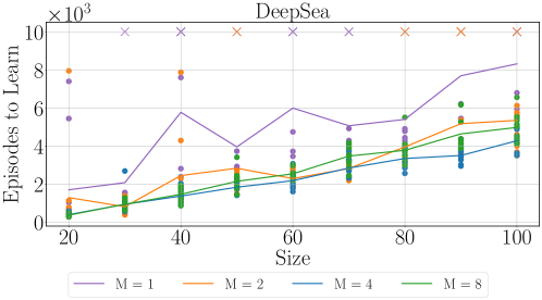
Figure 7: Ablation results on the impact of index dimension $M$. HyperAgent exhibits improved performance when $M$ exceeds 1, aligning with our theoretical analysis.

Ablation experiment on different sampling schemes for ${\bm{\xi}}$.

We have two sampling schemes for ${\bm{\xi}}$ in the computation of the $Q$-target and action selection: state-independent ${\bm{\xi}}$ sampling and state-dependent ${\bm{\xi}}$ sampling, see detailed description in Appendix C.2. In our implementation by default, HyperAgent employs the state-independent ${\bm{\xi}}$ for action selection, where we use the same index ${\bm{\xi}}_{k}(S)=\xi_{k}$ for each state within episode $k$. Whereas, HyperAgent utilizes state-dependent ${\bm{\xi}}$ for $Q$-target computation, where we sample independent $\xi\sim P_{\xi}$ when computing the $Q$-target for each transition tuple in mini-batches. To systematically compare the index sampling schemes on action selection and $Q$-target computation, two variants are created.

• HyperAgent with state-independent ${\bm{\xi}}$: applying state-independent ${\bm{\xi}}$ sampling to both $Q$-target computation and action selection.

• HyperAgent with state-dependent ${\bm{\xi}}$: applying state-dependent ${\bm{\xi}}$ sampling to both $Q$-target computation and action selection.

As illustrated in Figure 8, these distinct index sampling schemes for ${\bm{\xi}}$ exhibit nearly identical performance.

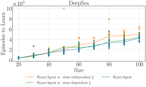
Figure 8: Ablation results for the sampling schemes used in $Q$-target computation. Both sampling schemes achieve similar performance.

Comparative results on optimistic index sampling.

Introduced in C.2, optimistic index sampling (OIS) for action selection and $Q$-target computation is another index sampling scheme in HyperAgent framework, naming HyperAgent w. OIS. As shown in Figure LABEL:fig:deepsea_ois(a), HyperAgent w. OIS outperforms HyperAgent by leveraging the OIS method to generate more optimistic estimates, thereby enhancing exploration. The OIS method incurs minimal additional computation, as we have set the dimension $M$ to 4.

The empirical implementation of LSVI-PHE (Ishfaq et al., 2021) also utilizes the similar optimistic sampling (OS) method with ensemble networks as described in Appendix A. Since no official implementation of LSVI-PHE is available, we apply the OIS to the Ensemble+ (Osband et al., 2018; 2019b), denoted as Ensemble+ w. OS, representing the LSVI-PHE. A critical difference between LSVI-PHE and HyperAgent w. OIS is that LSVI-PHE performs maximum value over $M$ separately trained ensemble models, while HyperAgent w. OIS has the computation advantage that we can sample as many as indices from reference distribution $P_{\xi}$ to form the optimistic estimation of value function even when the index dimension $M$ is small.

When $M=4$, both Ensemble+ and Ensemble+ w. OS demonstrates subpar performance. According to Osband et al. (2018) and the observation in LABEL:fig:deepsea_ois, a larger ensemble size ($M=16$) can lead to improved performance. When $M=16$, both Ensemble+ w. OS (LSVI-PHE) has a bit better performance compared with Ensemble+. The result of Ensemble+ w. OS ($M=16$) and HyperAgent w. OIS demonstrates enhanced deep exploration via optimistic value estimation, which is aligned with our theoretical insights.

In another dimension of comparison, As depicted in Figure LABEL:fig:deepsea_ois(b), Ensemble+ w. OS ($M=16$) still fails to solve the large-size DeepSea. This further showcases the exploration efficiency of HyperAgent.

E.2 Ablation studies on implementation settings and hyper-parameters

Sampling-based approximation.

HyperAgent by default uses Gaussian reference distribution $P_{\xi}=N(0,I_{M})$, which requires sampling-based approximation Equations 3 and 4. Therefore, it is imperative to set the number of indices $|\tilde{\Xi}|$ of Equation 4 to be sufficiently large for a good approximation given index dimension $M$. $|\tilde{\Xi}|=20$ falls short of delivering satisfactory results when $M=16$ as illustrated in Figure 11. For this scenario, increasing the number of indices $|\tilde{\Xi}|$ can alleviate performance degradation as depicted in Figure 11, facilitating deep exploration empirically. To achieve accurate approximation, $|\tilde{\Xi}|$ may need to grow exponentially with $M$, but this comes at the cost of increased computation. To balance accuracy and computation, we have chosen $M=4$ and $|\tilde{\Xi}|=20$ as the default hyper-parameters, which already demonstrate superior performance in Figure 2.

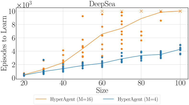
Figure 10: Results of HyperAgent with large index dimension. In both settings, we set $|\tilde{\Xi}|=20$, which fails to achieve satisfactory performance for $M=16$.

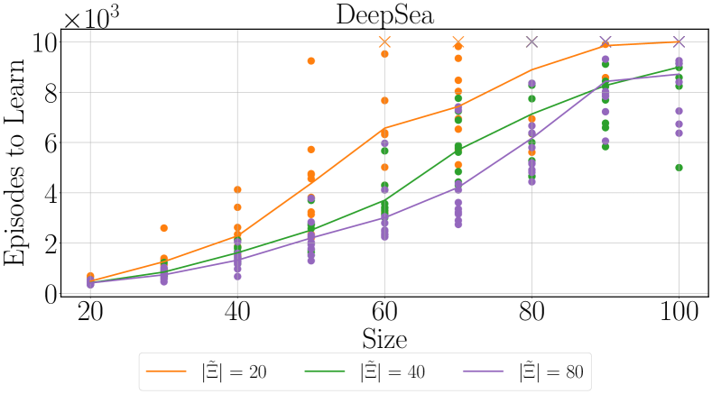
Figure 11: Results of HyperAgent with index dimension $M=16$. We can increase the number of indices $|\tilde{\Xi}|$ to alleviate performance degradation,

Ablation results for other hyper-parameters.

In addition, we have also investigated the effect of the $\sigma$ of Equation 2 on our method, as shown in Figure 12. HyperAgent is not sensitive to this hyper-parameter, and we have selected $\sigma=0.0001$ as the default hyper-parameter.

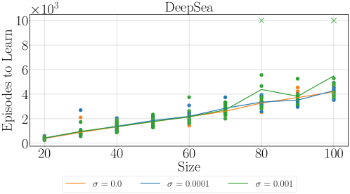
Figure 12: Ablation results on the $\sigma=0.0001$ of Equation 2. We set $\sigma=0.0001$ as the default setting.

E.3 Additional results with algorithms using hypermodel framework

Experiment investigating different network structures within the hypermodel framework.

We perform an ablation experiment examining various network structures, (1) HyperModel (Dwaracherla et al., 2020) (2) epinet (Osband et al., 2023a), outlined in Section C.3.2 with the same hyper-parameters, same algorithmic update rule, same target computation rule and same action selection rule.

The comparison results are presented in Figure 13. HyperModel is unable to solve DeepSea, even with a size of 20, while ENNDQN cannot solve DeepSea when the size exceeds 30. Overall, HyperAgent demonstrates superb efficiency and scalability, as it efficiently solves DeepSea instances of size $100^{2}$ that previous literature has never achieved.

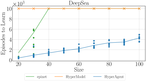
Figure 13: Results from various network structures using the hypermodel framework. HyperAgent demonstrates superior data and computational efficiency compared to other methods.

Ablation experiment on $Q$-target computation.

Several methods, including HyperDQN, ENNDQN, and Ensemble+, employ the injected index to achieve posterior approximation and utilize the same index to compute the $Q$-target as described in Section C.3.2. They apply the same index for both main $Q$-value and target $Q$-value computation, which we refer to as dependent $Q$-target computation. In contrast, HyperAgent employs independent $Q$-target computation, where it independently samples different indices to compute the target $Q$-value, a strategy supported by theoretical analysis. We contrast these two $Q$-target computation methods within the HyperAgent framework and introduce the HyperAgent w. dependent $Q$-target. As depicted in Figure 14, HyperAgent w. dependent $Q$-target demonstrates improved results, prompting further analysis of the underlying reasons in future research.

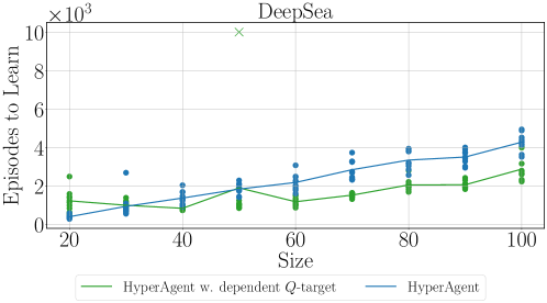
Figure 14: Ablation results on different $Q$-target computation methods. The method of dependent $Q$-target computation can achieve better results inspiring future research.

Appendix F Additional Results on Atari

We demonstrated the efficiency of HyperAgent in handling data and computation in Section 4.2. Here, we present comprehensive results for each environment to further establish the superiority of our approach.

Detailed results on each game.

We adhere to the evaluation protocol described in Section B.1 to obtain the best score achieved in each game with 2M steps of HyperAgent, as presented in Table 7. The sources of the compared baseline results can also be found in Section B.2.

Game Random Human DDQN^† DER Rainbow HyperDQN HyperAgent Alien 227.8 7127.7 722.7 1642.2 1167.1 862.0 1830.2 Amidar 5.8 1719.5 61.4 476.0 374.0 140.0 800.4 Assault 222.4 742.0 815.3 488.3 2725.2 494.2 3276.2 Asterix 210.0 8503.3 2471.1 1305.3 3213.3 713.3 2370.2 BankHeist 14.2 753.1 7.4 460.5 411.1 272.7 430.3 BattleZone 2360.0 37187.5 3925.0 19202.5 19379.7 11266.7 29399.0 Boxing 0.1 12.1 26.7 1.7 69.9 6.8 74.0 Breakout 1.7 30.5 2.0 6.5 137.3 11.9 54.8 ChopperCommand 811.0 7387.8 354.6 1488.9 1769.4 846.7 2957.2 CrazyClimber 10780.5 35829. 53166.5 36311.1 110215.8 42586.7 121855.8 DemonAttack 152.1 1971.0 1030.8 955.3 45961.3 2197.7 5852.0 Freeway 0.0 29.6 5.1 32.8 32.4 30.9 32.2 Frostbite 65.2 4334.7 358.3 3628.3 3648.7 724.7 4583.9 Gopher 257.6 2412.5 569.8 742.1 4938.0 1880.0 7365.8 Hero 1027.0 30826.4 2772.9 15409.4 11202.3 9140.3 12324.7 Jamesbond 29.0 302.8 15.0 462.1 773.1 386.7 951.6 Kangaroo 52.0 3035.0 134.9 8852.3 6456.1 3393.3 8517.1 Krull 1598.0 2665.5 6583.3 3786.7 8328.5 5488.7 8222.6 KungFuMaster 258.5 22736.3 12497.2 15457.0 25257.8 12940.0 23821.2 MsPacman 307.3 6951.6 1912.3 2333.7 1861.1 1305.3 3182.3 Pong -20.7 14.6 -15.4 20.6 5.1 20.5 20.5 PrivateEye 24.9 69571.3 37.8 900.9 100.0 64.5 171.9 Qbert 163.9 13455.0 1319.4 12345.5 7885.3 5793.3 12021.9 RoadRunner 11.5 7845.0 3693.5 14663.0 33851.0 7000.0 28789.4 Seaquest 68.4 42054.7 367.6 662.0 1524.7 370.7 2732.4 UpNDown 533.4 11693.2 3422.8 6806.3 39187.1 4080.7 19719.2

Table 7: The averaged score over 200 evaluation episodes for the best policy in hindsight (after 2M steps) for 26 Atari games. The performance of the random policy and the human expert is from dqn_zoo Quan & Ostrovski (2020).

We also present the relative improvement of HyperAgent in comparison to other baselines for each game, which is determined by the given following equation as per (Wang et al., 2016):

$$\text{relative improvement}=\frac{\text{proposed}-\text{baseline}}{\max(\text{human},\text{baseline})-\text{human}}.$$

Our classification of environments into three groups, namely “hard exploration (dense reward)”, “hard exploration (sparse reward)” and “easy exploration”, is based on the taxonomy proposed by Bellemare et al. (2016). The overall results are illustrated in Figures 15, 15, 16, 17 and 18.

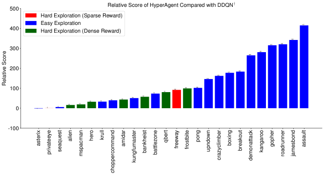
Figure 15: Relative improvement of HyperAgent compared with DDQN^†

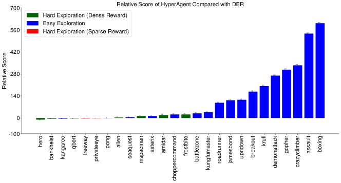
Figure 16: Relative improvement of HyperAgent compared with DER

Figure 17: Relative improvement of HyperAgent compared with HyperDQN

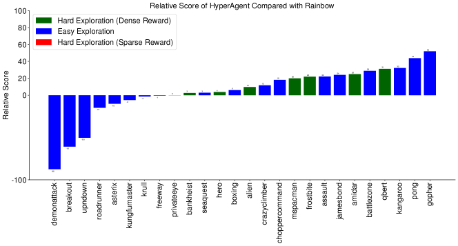
Figure 18: Relative improvement of HyperAgent compared with Rainbow

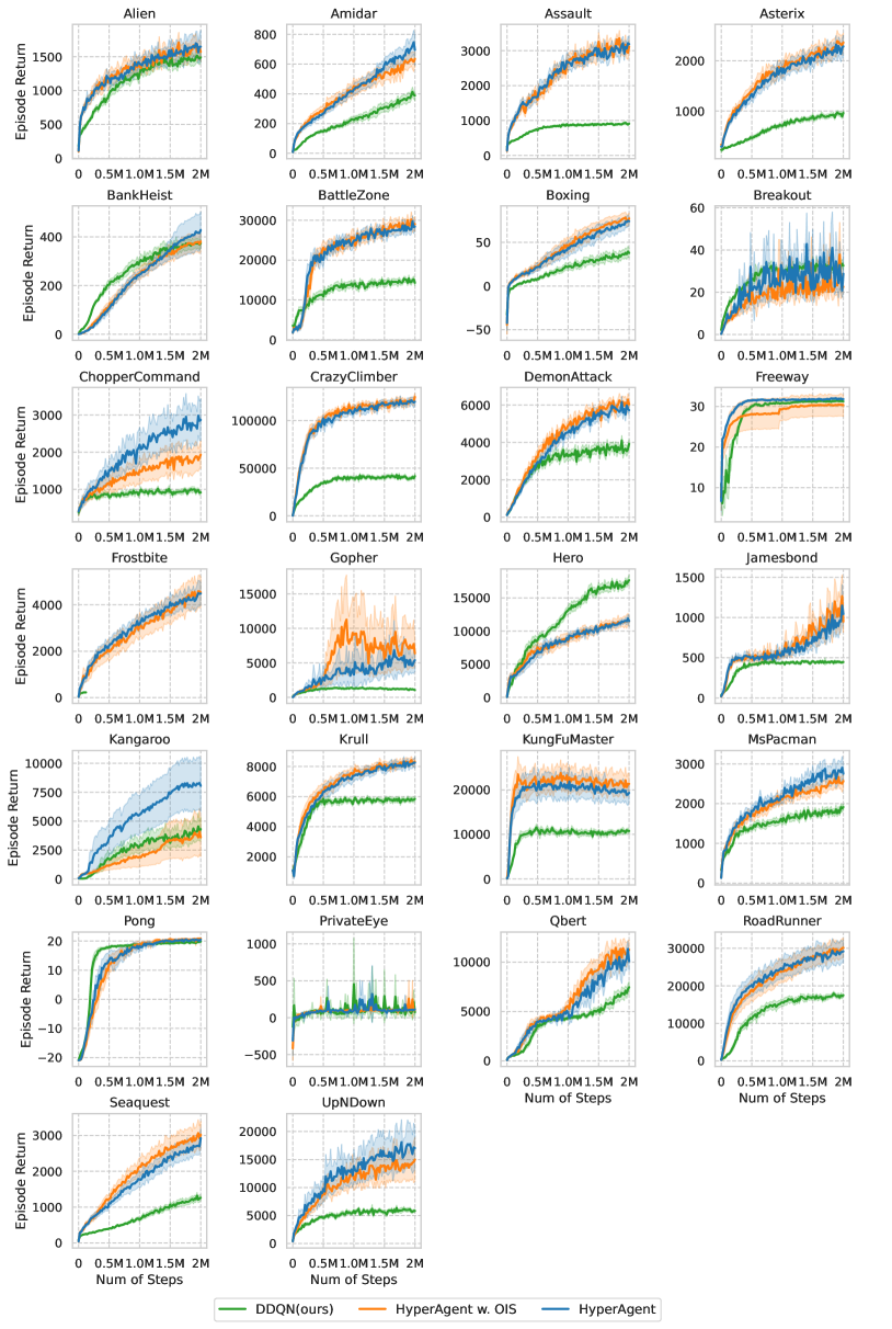
Figure 19: Learning curve for each game.

HyperAgent algorithm exhibits significant improvement compared to DDQN^†, DER, and HyperDQN in environments with “easy exploration”, and overall it performs better in all environments. This indicates that HyperAgent has better generalization and exploration abilities. On the other hand, when compared to Rainbow, our algorithm performs better in environments which are in the group of “hard exploration (dense reward)”, demonstrating its superior exploration capabilities. In the case of Freeway, which belongs to the “hard exploration (sparse reward)” group, both HyperAgent and Rainbow achieve similar optimal scores (as shown in Table 7). However, HyperAgent demonstrates faster convergence, as evidenced in Figure 3. Overall, HyperAgent showcases better generalization and exploration efficiency than other baselines.

We also evaluate the OIS method across the 26 Atari games, as illustrated in Table 8. Our findings indicate that the OIS method does not generate significant differences in complex networks like Convolutional layers.

Method	IQM	Median	Mean
HyperAgent	1.22 (1.15, 1.30)	1.07 (1.03, 1.14)	1.97 (1.89, 2.07)
HyperAgent w. OIS	1.15 (1.09, 1.22)	1.12 (1.02, 1.18)	2.02 (1.91, 2.16)

Table 8: Comparable results achieved using the OIS method in Atari games. The data in parentheses represent the 95% confidence interval.

Furthermore, we present the learning curve for each game in Figure 19. It is evident that HyperAgent has demonstrated superior performance compared to DDQN(ours), attributed to the integration of hypermodel that enhances exploration. Moreover, it is worth highlighting that the learning curve of HyperAgent continues to rise in specific environments, indicating that it can achieve even better performance with additional training.

Additional results about exploration on Atari.

To further demonstrate the exploration efficiency of HyperAgent, we compare it with additional baselines, including AdamLMCDQN (Ishfaq et al., 2023), LangevinAdam (Dwaracherla & Van Roy, 2020), HyperDQN (Li et al., 2022a) and our variant HyperAgent w. OIS. As depicted in Figure 20, both HyperDQN and HyperAgent demonstrate improved results, indicating that applying hypermodel can lead to better posterior approximation and consequently enhance exploration.

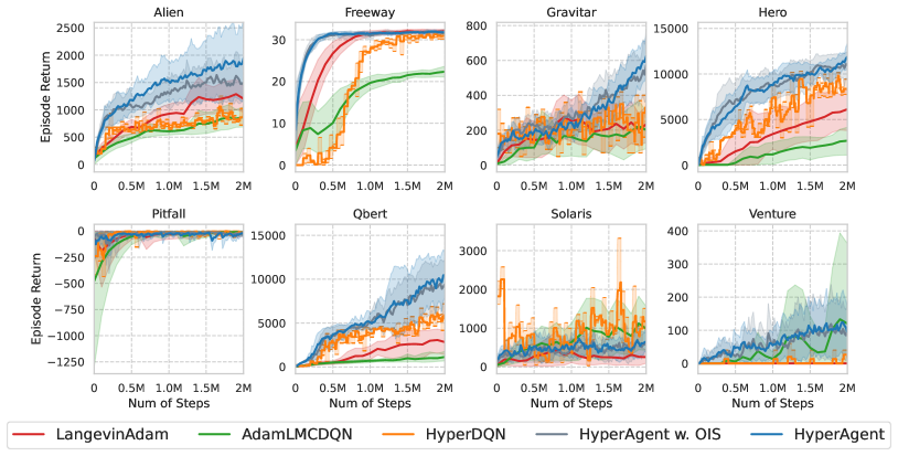
Figure 20: Comparative results on 8 hardest exploration games with more baselines.

Additional results on other 29 Atari games.

To further showcase the robustness and scalability of HyperAgent, we conduct experiments on all 55 Atari games using identical settings (see Table 4). We present the best score achieved in these 29 environments using 2M steps in Table 9, with 5 seeds repeated for each environment. HyperAgent outperforms others in over half of these 29 environments, delivering top performance in 31 out of 55 Atari games.

Game Random Human DDQN^† Rainbow HyperDQN HyperAgent Asteroids 210.0 47388.7 520.8 969.4 1044.7 1176.6 Atlantis 12850.0 29028.1 5771.3 528642.7 370160.0 793851.9 BeamRider 363.9 16926.5 464.4 10408.0 981.9 6749.2 Berzerk 123.7 2630.4 566.6 822.7 336.7 840.5 Bowling 23.1 160.7 12.6 27.7 14.8 61.3 Centipede 2090.9 12017.0 4343.2 5352.1 2071.5 4121.9 Defender 2874.5 18688.9 2978.4 25457.1 4063.3 21422.7 DoubleDunk -18.6 -16.4 -21.2 -2.2 -17.7 -1.7 Enduro 0.0 860.5 338.7 1496.6 201.0 1223.0 FishingDerby -91.7 -38.7 -78.1 -22.4 -74.3 -0.7 Gravitar 173.0 3351.4 2.6 372.0 300.0 629.5 IceHockey -11.2 0.9 -12.4 -7.0 -11.6 -3.8 NameThisGame 2292.3 8049.0 5870.3 9547.2 3628.0 5916.4 Phoenix 761.4 7242.6 3806.2 6325.0 3270.0 4941.9 Pitfall -229.4 6463.7 -55.5 -0.1 -13.0 -11.2 Riverraid 1338.5 17118.0 3406.2 5627.9 4233.3 6896.3 Robotank 2.2 11.9 7.8 22.4 3.1 37.2 Skiing -17098.1 -4336.9 -22960.7 -16884.8 -29975.0 -11654.4 Solaris 1236.3 12326.7 390.2 1185.9 1173.3 941.3 SpaceInvaders 148.0 1668.7 356.1 742.2 425.3 762.2 StarGunner 664.0 10250.0 346.3 11142.3 1113.3 6135.7 Tennis -23.8 -8.3 -10.1 0.0 -17.0 -1.4 TimePilot 3568.0 5229.2 2204.6 3763.8 3106.7 6006.1 Tutankham 11.4 167.6 108.6 104.1 93.0 116.2 Venture 0.0 1187.5 21.5 0.0 26.7 163.9 VideoPinball 16256.9 17667.9 10557.5 49982.2 24859.2 29674.8 WizardOfWor 563.5 4756.5 275.7 3770.9 1393.3 4019.5 YarsRevenge 3092.9 54576.9 10485.5 10195.6 4263.1 28805.5 Zaxxon 32.5 9173.3 2.1 7344.1 3093.3 7688.1

Table 9: The evaluated score of other 29 games from ALE suite.

References

- Agarwal et al. (2023) Alekh Agarwal, Yujia Jin, and Tong Zhang. Vo l: Towards optimal regret in model-free rl with nonlinear function approximation. In The Thirty Sixth Annual Conference on Learning Theory, pp. 987–1063. PMLR, 2023.
- Agarwal et al. (2021) Rishabh Agarwal, Max Schwarzer, Pablo Samuel Castro, Aaron C Courville, and Marc Bellemare. Deep reinforcement learning at the edge of the statistical precipice. Advances in neural information processing systems, 34:29304–29320, 2021.
- Anonymous (2024) Anonymous. Provable and practical: Efficient exploration in reinforcement learning via langevin monte carlo. In The Twelfth International Conference on Learning Representations, 2024. URL https://openreview.net/forum?id=nfIAEJFiBZ.
- Aravindan & Lee (2021) Siddharth Aravindan and Wee Sun Lee. State-aware variational thompson sampling for deep q-networks. In Proceedings of the 20th International Conference on Autonomous Agents and MultiAgent Systems, pp. 124–132, 2021.
- Azar et al. (2017) Mohammad Gheshlaghi Azar, Ian Osband, and Rémi Munos. Minimax regret bounds for reinforcement learning. In International Conference on Machine Learning, pp. 263–272. PMLR, 2017.
- Bai et al. (2021) Chenjia Bai, Lingxiao Wang, Lei Han, Jianye Hao, Animesh Garg, Peng Liu, and Zhaoran Wang. Principled exploration via optimistic bootstrapping and backward induction. In International Conference on Machine Learning, pp. 577–587. PMLR, 2021.
- Bellemare et al. (2016) Marc Bellemare, Sriram Srinivasan, Georg Ostrovski, Tom Schaul, David Saxton, and Remi Munos. Unifying count-based exploration and intrinsic motivation. Advances in neural information processing systems, 29, 2016.
- Bellemare et al. (2013) Marc G Bellemare, Yavar Naddaf, Joel Veness, and Michael Bowling. The arcade learning environment: An evaluation platform for general agents. Journal of Artificial Intelligence Research, 47:253–279, 2013.
- Bellemare et al. (2017) Marc G Bellemare, Will Dabney, and Rémi Munos. A distributional perspective on reinforcement learning. In International conference on machine learning, pp. 449–458. PMLR, 2017.
- Bertsekas & Tsitsiklis (1996) Dimitri Bertsekas and John N Tsitsiklis. Neuro-dynamic programming. Athena Scientific, 1996.
- Cagatan (2023) Omer Veysel Cagatan. Barlowrl: Barlow twins for data-efficient reinforcement learning. arXiv preprint arXiv:2308.04263, 2023.
- Dann et al. (2022) Chris Dann, Yishay Mansour, Mehryar Mohri, Ayush Sekhari, and Karthik Sridharan. Guarantees for epsilon-greedy reinforcement learning with function approximation. In International conference on machine learning, pp. 4666–4689. PMLR, 2022.
- Dann et al. (2021) Christoph Dann, Mehryar Mohri, Tong Zhang, and Julian Zimmert. A provably efficient model-free posterior sampling method for episodic reinforcement learning. Advances in Neural Information Processing Systems, 34:12040–12051, 2021.
- Du et al. (2021) Simon Du, Sham Kakade, Jason Lee, Shachar Lovett, Gaurav Mahajan, Wen Sun, and Ruosong Wang. Bilinear classes: A structural framework for provable generalization in rl. In International Conference on Machine Learning, pp. 2826–2836. PMLR, 2021.
- Dwaracherla & Van Roy (2020) Vikranth Dwaracherla and Benjamin Van Roy. Langevin dqn. arXiv preprint arXiv:2002.07282, 2020.
- Dwaracherla et al. (2020) Vikranth Dwaracherla, Xiuyuan Lu, Morteza Ibrahimi, Ian Osband, Zheng Wen, and Benjamin Van Roy. Hypermodels for exploration. In International Conference on Learning Representations, 2020. URL https://openreview.net/forum?id=ryx6WgStPB.
- Ernst et al. (2005) Damien Ernst, Pierre Geurts, and Louis Wehenkel. Tree-based batch mode reinforcement learning. Journal of Machine Learning Research, 6, 2005.
- Fortunato et al. (2017) Meire Fortunato, Mohammad Gheshlaghi Azar, Bilal Piot, Jacob Menick, Ian Osband, Alex Graves, Vlad Mnih, Remi Munos, Demis Hassabis, Olivier Pietquin, et al. Noisy networks for exploration. arXiv preprint arXiv:1706.10295, 2017.
- Foster et al. (2021) Dylan J Foster, Sham M Kakade, Jian Qian, and Alexander Rakhlin. The statistical complexity of interactive decision making. arXiv preprint arXiv:2112.13487, 2021.
- Hafner et al. (2023) Danijar Hafner, Jurgis Pasukonis, Jimmy Ba, and Timothy Lillicrap. Mastering diverse domains through world models. arXiv preprint arXiv:2301.04104, 2023.
- Hessel et al. (2018) Matteo Hessel, Joseph Modayil, Hado Van Hasselt, Tom Schaul, Georg Ostrovski, Will Dabney, Dan Horgan, Bilal Piot, Mohammad Azar, and David Silver. Rainbow: Combining improvements in deep reinforcement learning. In Proceedings of the AAAI conference on artificial intelligence, volume 32, 2018.
- Ishfaq et al. (2021) Haque Ishfaq, Qiwen Cui, Viet Nguyen, Alex Ayoub, Zhuoran Yang, Zhaoran Wang, Doina Precup, and Lin Yang. Randomized exploration in reinforcement learning with general value function approximation. In International Conference on Machine Learning, pp. 4607–4616. PMLR, 2021.
- Ishfaq et al. (2023) Haque Ishfaq, Qingfeng Lan, Pan Xu, A. Rupam Mahmood, Doina Precup, Anima Anandkumar, and Kamyar Azizzadenesheli. Provable and practical: Efficient exploration in reinforcement learning via langevin monte carlo, 2023.
- Jaksch et al. (2010) Thomas Jaksch, Ronald Ortner, and Peter Auer. Near-optimal regret bounds for reinforcement learning. Journal of Machine Learning Research, 11:1563–1600, 2010.
- Jiang et al. (2017) Nan Jiang, Akshay Krishnamurthy, Alekh Agarwal, John Langford, and Robert E Schapire. Contextual decision processes with low bellman rank are pac-learnable. In International Conference on Machine Learning, pp. 1704–1713. PMLR, 2017.
- Jin et al. (2020) Chi Jin, Zhuoran Yang, Zhaoran Wang, and Michael I Jordan. Provably efficient reinforcement learning with linear function approximation. In Conference on Learning Theory, pp. 2137–2143. PMLR, 2020.
- Jin et al. (2021) Chi Jin, Qinghua Liu, and Sobhan Miryoosefi. Bellman eluder dimension: New rich classes of rl problems, and sample-efficient algorithms. Advances in neural information processing systems, 34:13406–13418, 2021.
- Johnson & Lindenstrauss (1984) William B Johnson and Joram Lindenstrauss. Extensions of lipschitz mappings into a hilbert space. In Conference on Modern Analysis and Probability, volume 26, pp. 189–206. American Mathematical Society, 1984.
- Kaiser et al. (2019) Lukasz Kaiser, Mohammad Babaeizadeh, Piotr Milos, Blazej Osinski, Roy H Campbell, Konrad Czechowski, Dumitru Erhan, Chelsea Finn, Piotr Kozakowski, Sergey Levine, et al. Model-based reinforcement learning for atari. arXiv preprint arXiv:1903.00374, 2019.
- Kakade (2003) Sham Machandranath Kakade. On the sample complexity of reinforcement learning. University of London, University College London (United Kingdom), 2003.
- Kearns & Singh (2002) Michael Kearns and Satinder Singh. Near-optimal reinforcement learning in polynomial time. Machine learning, 49:209–232, 2002.
- Lai & Robbins (1985) Tze Leung Lai and Herbert Robbins. Asymptotically efficient adaptive allocation rules. Advances in applied mathematics, 6(1):4–22, 1985.
- Laskin et al. (2020) Michael Laskin, Aravind Srinivas, and Pieter Abbeel. Curl: Contrastive unsupervised representations for reinforcement learning. In International Conference on Machine Learning, pp. 5639–5650. PMLR, 2020.
- Li (2024a) Yingru Li. Probability tools for sequential random projection, 2024a. URL https://arxiv.org/abs/2402.14026.
- Li (2024b) Yingru Li. Simple, unified analysis of johnson-lindenstrauss with applications, 2024b. URL https://arxiv.org/abs/2402.10232.
- Li et al. (2022a) Ziniu Li, Yingru Li, Yushun Zhang, Tong Zhang, and Zhi-Quan Luo. HyperDQN: A randomized exploration method for deep reinforcement learning. In International Conference on Learning Representations, 2022a. URL https://openreview.net/forum?id=X0nrKAXu7g-.
- Li et al. (2022b) Ziniu Li, Tian Xu, and Yang Yu. A note on target q-learning for solving finite mdps with a generative oracle. arXiv preprint arXiv:2203.11489, 2022b.
- Liu & Abbeel (2021) Hao Liu and Pieter Abbeel. Aps: Active pretraining with successor features. In International Conference on Machine Learning, pp. 6736–6747. PMLR, 2021.
- Liu et al. (2023) Zhihan Liu, Miao Lu, Wei Xiong, Han Zhong, Hao Hu, Shenao Zhang, Sirui Zheng, Zhuoran Yang, and Zhaoran Wang. Maximize to explore: One objective function fusing estimation, planning, and exploration. In Thirty-seventh Conference on Neural Information Processing Systems, 2023. URL https://openreview.net/forum?id=A57UMlUJdc.
- Lu & Van Roy (2019) Xiuyuan Lu and Benjamin Van Roy. Information-theoretic confidence bounds for reinforcement learning. In H. Wallach, H. Larochelle, A. Beygelzimer, F. d'Alché-Buc, E. Fox, and R. Garnett (eds.), Advances in Neural Information Processing Systems, volume 32. Curran Associates, Inc., 2019. URL https://proceedings.neurips.cc/paper/2019/file/411ae1bf081d1674ca6091f8c59a266f-Paper.pdf.
- Lu et al. (2023) Xiuyuan Lu, Benjamin Van Roy, Vikranth Dwaracherla, Morteza Ibrahimi, Ian Osband, Zheng Wen, et al. Reinforcement learning, bit by bit. Foundations and Trends® in Machine Learning, 16(6):733–865, 2023.
- Mnih et al. (2015) Volodymyr Mnih, Koray Kavukcuoglu, David Silver, Andrei A Rusu, Joel Veness, Marc G Bellemare, Alex Graves, Martin Riedmiller, Andreas K Fidjeland, Georg Ostrovski, et al. Human-level control through deep reinforcement learning. nature, 518(7540):529–533, 2015.
- Nikishin et al. (2022) Evgenii Nikishin, Max Schwarzer, Pierluca D’Oro, Pierre-Luc Bacon, and Aaron Courville. The primacy bias in deep reinforcement learning. In International conference on machine learning, pp. 16828–16847. PMLR, 2022.
- Osband & Van Roy (2015) Ian Osband and Benjamin Van Roy. Bootstrapped thompson sampling and deep exploration. arXiv preprint arXiv:1507.00300, 2015.
- Osband & Van Roy (2017) Ian Osband and Benjamin Van Roy. Why is posterior sampling better than optimism for reinforcement learning? In International conference on machine learning, pp. 2701–2710. PMLR, 2017.
- Osband et al. (2013) Ian Osband, Benjamin Van Roy, and Daniel Russo. (more) efficient reinforcement learning via posterior sampling. In Advances in Neural Information Processing Systems, pp. 3003–3011, 2013.
- Osband et al. (2016) Ian Osband, Charles Blundell, Alexander Pritzel, and Benjamin Van Roy. Deep exploration via bootstrapped dqn. Advances in neural information processing systems, 29, 2016.
- Osband et al. (2018) Ian Osband, John Aslanides, and Albin Cassirer. Randomized prior functions for deep reinforcement learning. Advances in Neural Information Processing Systems, 31, 2018.
- Osband et al. (2019a) Ian Osband, Yotam Doron, Matteo Hessel, John Aslanides, Eren Sezener, Andre Saraiva, Katrina McKinney, Tor Lattimore, Csaba Szepesvari, Satinder Singh, et al. Behaviour suite for reinforcement learning. arXiv preprint arXiv:1908.03568, 2019a.
- Osband et al. (2019b) Ian Osband, Benjamin Van Roy, Daniel J. Russo, and Zheng Wen. Deep exploration via randomized value functions. Journal of Machine Learning Research, 20(124):1–62, 2019b. URL http://jmlr.org/papers/v20/18-339.html.
- Osband et al. (2023a) Ian Osband, Zheng Wen, Seyed Mohammad Asghari, Vikranth Dwaracherla, Morteza Ibrahimi, Xiuyuan Lu, and Benjamin Van Roy. Epistemic neural networks. In Thirty-seventh Conference on Neural Information Processing Systems, 2023a. URL https://openreview.net/forum?id=dZqcC1qCmB.
- Osband et al. (2023b) Ian Osband, Zheng Wen, Seyed Mohammad Asghari, Vikranth Dwaracherla, Morteza Ibrahimi, Xiuyuan Lu, and Benjamin Van Roy. Approximate thompson sampling via epistemic neural networks. In Proceedings of the Thirty-Ninth Conference on Uncertainty in Artificial Intelligence, UAI ’23. JMLR.org, 2023b.
- Plappert et al. (2017) Matthias Plappert, Rein Houthooft, Prafulla Dhariwal, Szymon Sidor, Richard Y Chen, Xi Chen, Tamim Asfour, Pieter Abbeel, and Marcin Andrychowicz. Parameter space noise for exploration. arXiv preprint arXiv:1706.01905, 2017.
- Qin et al. (2022) Chao Qin, Zheng Wen, Xiuyuan Lu, and Benjamin Van Roy. An analysis of ensemble sampling. arXiv preprint arXiv:2203.01303, 2022.
- Quan & Ostrovski (2020) John Quan and Georg Ostrovski. DQN Zoo: Reference implementations of DQN-based agents, 2020. URL http://github.com/deepmind/dqn_zoo.
- Russo & Van Roy (2018) Daniel Russo and Benjamin Van Roy. Learning to optimize via information-directed sampling. Operations Research, 66(1):230–252, 2018.
- Russo et al. (2018) Daniel J Russo, Benjamin Van Roy, Abbas Kazerouni, Ian Osband, Zheng Wen, et al. A tutorial on thompson sampling. Foundations and Trends® in Machine Learning, 11(1):1–96, 2018.
- Schrittwieser et al. (2020) Julian Schrittwieser, Ioannis Antonoglou, Thomas Hubert, Karen Simonyan, Laurent Sifre, Simon Schmitt, Arthur Guez, Edward Lockhart, Demis Hassabis, Thore Graepel, et al. Mastering atari, go, chess and shogi by planning with a learned model. Nature, 588(7839):604–609, 2020.
- Schwarzer et al. (2020) Max Schwarzer, Ankesh Anand, Rishab Goel, R Devon Hjelm, Aaron Courville, and Philip Bachman. Data-efficient reinforcement learning with self-predictive representations. arXiv preprint arXiv:2007.05929, 2020.
- Schwarzer et al. (2023) Max Schwarzer, Johan Samir Obando Ceron, Aaron Courville, Marc G Bellemare, Rishabh Agarwal, and Pablo Samuel Castro. Bigger, better, faster: Human-level atari with human-level efficiency. In International Conference on Machine Learning, pp. 30365–30380. PMLR, 2023.
- Strehl (2007) Alexander L Strehl. Probably approximately correct (PAC) exploration in reinforcement learning. PhD thesis, Rutgers University-Graduate School-New Brunswick, 2007.
- Strens (2000) Malcolm Strens. A bayesian framework for reinforcement learning. In International Conference on Machine Learning, pp. 943–950, 2000.
- Sutton & Barto (2018) Richard S Sutton and Andrew G Barto. Reinforcement learning: An introduction. MIT press, 2018.
- Thompson (1933) William R Thompson. On the likelihood that one unknown probability exceeds another in view of the evidence of two samples. Biometrika, 25(3/4):285–294, 1933.
- Thrun (1992) Sebastian Thrun. Efficient exploration in reinforcement learning. Technical Report CMU-CS-92-102, Carnegie Mellon University, Pittsburgh, PA, January 1992.
- Tiapkin et al. (2022) Daniil Tiapkin, Denis Belomestny, Éric Moulines, Alexey Naumov, Sergey Samsonov, Yunhao Tang, Michal Valko, and Pierre Ménard. From dirichlet to rubin: Optimistic exploration in rl without bonuses. In International Conference on Machine Learning, pp. 21380–21431. PMLR, 2022.
- Van Hasselt et al. (2016) Hado Van Hasselt, Arthur Guez, and David Silver. Deep reinforcement learning with double q-learning. In Proceedings of the AAAI conference on artificial intelligence, volume 30, 2016.
- Van Hasselt et al. (2019) Hado P Van Hasselt, Matteo Hessel, and John Aslanides. When to use parametric models in reinforcement learning? Advances in Neural Information Processing Systems, 32, 2019.
- Wang et al. (2020) Ruosong Wang, Russ R Salakhutdinov, and Lin Yang. Reinforcement learning with general value function approximation: Provably efficient approach via bounded eluder dimension. Advances in Neural Information Processing Systems, 33:6123–6135, 2020.
- Wang et al. (2016) Ziyu Wang, Tom Schaul, Matteo Hessel, Hado Hasselt, Marc Lanctot, and Nando Freitas. Dueling network architectures for deep reinforcement learning. In International conference on machine learning, pp. 1995–2003. PMLR, 2016.
- Watkins & Dayan (1992) Christopher JCH Watkins and Peter Dayan. Q-learning. Machine learning, 8:279–292, 1992.
- Welling & Teh (2011) Max Welling and Yee W Teh. Bayesian learning via stochastic gradient langevin dynamics. In Proceedings of the 28th international conference on machine learning (ICML-11), pp. 681–688, 2011.
- Wen (2014) Zheng Wen. Efficient reinforcement learning with value function generalization. Stanford University, 2014.
- Xu et al. (2022) Pan Xu, Hongkai Zheng, Eric V Mazumdar, Kamyar Azizzadenesheli, and Animashree Anandkumar. Langevin monte carlo for contextual bandits. In International Conference on Machine Learning, pp. 24830–24850. PMLR, 2022.
- Ye et al. (2021) Weirui Ye, Shaohuai Liu, Thanard Kurutach, Pieter Abbeel, and Yang Gao. Mastering atari games with limited data. Advances in Neural Information Processing Systems, 34:25476–25488, 2021.
- Zhang (2022) Tong Zhang. Feel-good thompson sampling for contextual bandits and reinforcement learning. SIAM Journal on Mathematics of Data Science, 4(2):834–857, 2022.
- Zhong et al. (2022) Han Zhong, Wei Xiong, Sirui Zheng, Liwei Wang, Zhaoran Wang, Zhuoran Yang, and Tong Zhang. Gec: A unified framework for interactive decision making in mdp, pomdp, and beyond. arXiv preprint arXiv:2211.01962, 2022.