Abstract

Transformer-based architectures achieved breakthrough performance in natural language processing and computer vision, yet they remain inferior to simpler linear baselines in multivariate long-term forecasting. To better understand this phenomenon, we start by studying a toy linear forecasting problem for which we show that transformers are incapable of converging to their true solution despite their high expressive power. We further identify the attention of transformers as being responsible for this low generalization capacity. Building upon this insight, we propose a shallow lightweight transformer model that successfully escapes bad local minima when optimized with sharpness-aware optimization. We empirically demonstrate that this result extends to all commonly used real-world multivariate time series datasets. In particular, SAMformer surpasses the current state-of-the-art model TSMixer by $\mathbf{14.33\%}$ on average, while having $\mathbf{\sim 4}$ times fewer parameters. The code is available at https://github.com/romilbert/samformer.

boxthm]Proposition boxthm]Example boxthm]Corollary boxthm]Lemma boxthm]Definition

 

 

Romain Ilbert^*$1$$2$                        Ambroise Odonnat^*1                        Vasilii Feofanov¹

Aladin Virmaux¹                        Giuseppe Paolo¹                        Themis Palpanas²                        Ievgen Redko¹

¹Huawei Noah’s Ark Lab                        ²LIPADE, Paris Descartes University

1 Introduction

Multivariate time series forecasting is a classical learning problem that consists of analyzing time series to predict future trends based on historical information. In particular, long-term forecasting is notoriously challenging due to feature correlations and long-term temporal dependencies in time series.

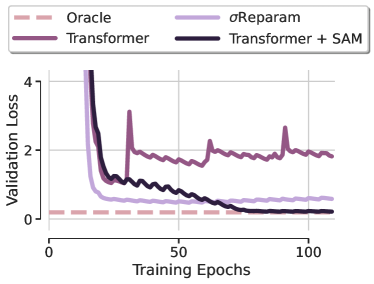
Figure 1: Illustration of our approach on synthetic data. Oracle is the optimal solution, Transformer is a base transformer, $\sigma$Reparam is a Transformer with weight rescaling (Zhai et al.,, 2023) and Transformer + SAM is Transformer trained with sharpness-aware minimization. Transformer overfits, $\sigma$Reparam improves slightly but fails to reach Oracle while Transformer+SAM generalizes perfectly. This motivates SAMformer, a shallow transformer combining SAM and best practices in time series forecasting.

This learning problem is prevalent in those real-world applications where observations are gathered sequentially, such as medical data (Čepulionis and Lukoševičiūtė,, 2016), electricity consumption (UCI, nd, ), temperatures (Max Planck Institute, nd, ), or stock prices (Sonkavde et al.,, 2023). A plethora of methods have been developed for this task, from classical mathematical tools (Sorjamaa et al.,, 2007; Chen and Tao,, 2021) and statistical approaches like ARIMA (Box and Jenkins,, 1990; Box et al.,, 1974) to more recent deep learning ones (Casolaro et al.,, 2023), including recurrent and convolutional neural networks (Rangapuram et al.,, 2018; Salinas et al.,, 2020; Fan et al.,, 2019; Lai et al., 2018a, ; Sen et al.,, 2019).

Recently, the transformer architecture (Vaswani et al.,, 2017) became ubiquitous in natural language processing (NLP) (Devlin et al.,, 2018; Radford et al.,, 2018; Touvron et al.,, 2023; OpenAI,, 2023) and computer vision (Dosovitskiy et al.,, 2021; Caron et al.,, 2021; Touvron et al.,, 2021), achieving breakthrough performance in both domains.

Transformers are known to be particularly efficient in dealing with sequential data, a property that naturally calls for their application on time series. Unsurprisingly, many works attempted to propose time series-specific transformer architectures to benefit from their capacity to capture temporal interactions (Zhou et al.,, 2021; Wu et al.,, 2021; Zhou et al.,, 2022; Nie et al.,, 2023). However, the current state-of-the-art in multivariate time series forecasting is achieved with a simpler MLP-based model (Chen et al.,, 2023), which significantly outperforms transformer-based methods. Moreover, Zeng et al., (2023) have recently found that linear networks can be on par or better than transformers for the forecasting task, questioning their practical utility. This curious finding serves as a starting point for our work.

Limitation of current approaches.

Recent works applying transformers to time series data have mainly focused on either (i) efficient implementations reducing the quadratic cost of attention  (Li et al.,, 2019; Liu et al.,, 2022; Cirstea et al.,, 2022; Kitaev et al.,, 2020; Zhou et al.,, 2021; Wu et al.,, 2021) or (ii) decomposing time series to better capture the underlying patterns in them (Wu et al.,, 2021; Zhou et al.,, 2022). Surprisingly, none of these works have specifically addressed a well-known issue of transformers related to their training instability, particularly present in the absence of large-scale data  (Liu et al.,, 2020; Dosovitskiy et al.,, 2021).

Trainability of transformers.

In computer vision and NLP, it has been found that attention matrices can suffer from entropy or rank collapse (Dong et al.,, 2021). Then, several approaches have been proposed to overcome these issues Chen et al., (2022); Zhai et al., (2023). However, in the case of time series forecasting, open questions remain about how transformer architectures can be trained effectively without a tendency to overfit. We aim to show that by eliminating training instability, transformers can excel in multivariate long-term forecasting, contrary to previous beliefs of their limitations.

Summary of our contributions.

Our proposal puts forward the following contributions:

1. We illustrate that transformers generalize poorly and converge to sharp local minima even on a simple toy linear forecasting problem. We further identify that attention is largely responsible for it;

2. We propose a shallow transformer model, termed SAMformer, that incorporates the best practices proposed in the research community including reversible instance normalization (RevIN, Kim et al., 2021b ) and channel-wise attention Zhang et al., (2022); Zamir et al., (2022) recently introduced in computer vision community. We show that optimizing such a simple transformer with sharpness-aware minimization (SAM) allows convergence to local minima with better generalization;

3. We empirically demonstrate the superiority of our approach on common multivariate long-term forecasting datasets. SAMformer improves the current state-of-the-art multivariate model TSMixer by $\mathbf{14.33\%}$ on average, while having $\mathbf{\sim 4}$ times fewer parameters.

2 Proposed Approach

Notations.

We represent scalar values with regular letters (e.g., parameter $\lambda$), vectors with bold lowercase letters (e.g., vector $\mathbf{x}$), and matrices with bold capital letters (e.g., matrix $\mathbf{M}$). We denote by $\mathbf{M}^{\top}$ the transpose of $\mathbf{M}$ and likewise for vectors. The rank of a matrix $\mathbf{M}$ is denoted by $\operatorname{rank}\left(\mathbf{M}\right)$, and its Frobenius norm by $\lVert\mathbf{M}\rVert_{\mathrm{F}}$. We let $\tilde{n}=\min\{n,m\}$, and denote by $\|\mathbf{M}\|_{*}=\sum_{i=1}^{\tilde{n}}\sigma_{i}(\mathbf{M})$ the nuclear norm of $\mathbf{M}$ with $\sigma_{i}(\mathbf{M})$ being its singular values, and by $\|\mathbf{M}\|_{2}=\sigma_{\max}(\mathbf{M})$ its spectral norm. The identity matrix of size $n\times n$ is denoted by $\mathbf{I}_{n}$. The notation $\mathbf{M}\succcurlyeq\mathbf{0}$ indicates that $\mathbf{M}$ is positive semi-definite.

2.1 Problem Setup

We consider the multivariate long-term forecasting framework: given a $D$-dimensional time series of length $L$ (look-back window), arranged in a matrix $\mathbf{X}\in\mathbb{R}^{D\times L}$ to facilitate channel-wise attention, our objective is to predict its next $H$ values (prediction horizon), denoted by $\mathbf{Y}\in\mathbb{R}^{D\times H}$. We assume that we have access to a training set that consists of $N$ observations $(\mathcal{X},\mathcal{Y})=(\{\mathbf{X}^{(i)}\}_{i=0}^{N},\ \{\mathbf{Y}^{(i)}\}_{i=0}^{N})$, and denote by $\mathbf{X}^{(i)}_{d}\in\mathbb{R}^{1\times L}$ (respectively  $\mathbf{Y}^{(i)}_{d}\in\mathbb{R}^{1\times H}$) the $d$-th feature of the $i$-th input (respectively target) time series. We aim to train a predictor $f_{\bm{\omega}}:\mathbb{R}^{D\times L}\to\mathbb{R}^{D\times H}$ parameterized by $\bm{\omega}$ that minimizes the mean squared error (MSE) on the training set:

$$\mathcal{L}_{\mathrm{train}}(\bm{\omega})=\frac{1}{ND}\sum_{i=0}^{N}\lVert\mathbf{Y}^{(i)}-f_{\bm{\omega}}(\mathbf{X}^{(i)})\rVert_{\mathrm{F}}^{2}\,.$$ (1)

2.2 Motivational Example

Recently, Zeng et al., (2023) showed that transformers perform on par with, or are worse than, simple linear neural networks trained to directly project the input to the output. We use this observation as a starting point by considering the following generative model for our toy regression problem mimicking a time series forecasting setup considered later:

$$\mathbf{Y}=\mathbf{X}\mathbf{W}_{\mathrm{toy}}+\bm{\varepsilon}.$$ (2)

We let $L\!=\!512,H\!=\!96,D\!=\!7$ and $\mathbf{W}_{\mathrm{toy}}\in\mathbb{R}^{L\times H},\bm{\epsilon}\in\mathbb{R}^{D\times H}$ having random normal entries and generate $15000$ input-target pairs $\left(\mathbf{X},\mathbf{Y}\right)$ ($10000$ for train and $5000$ for validation), with $\mathbf{X}\in\mathbb{R}^{D\times L}$ having random normal entries.

Given this generative model, we would like to develop a transformer architecture that can efficiently solve the problem in Eq. (2) without unnecessary complexity. To achieve this, we propose to simplify the usual transformer encoder by applying attention to $\mathbf{X}$ and incorporating a residual connection that adds $\mathbf{X}$ to the attention’s output. Instead of adding a feedforward block on top of this residual connection, we directly employ a linear layer for output prediction. Formally, our model is defined as follows:

$$f(\mathbf{X})=\left[\mathbf{X}+\mathbf{A}(\mathbf{X})\mathbf{X}\mathbf{W}_{V}\mathbf{W}_{O}\right]\mathbf{W},$$ (3)

with $\mathbf{W}\in\mathbb{R}^{L\times H},\mathbf{W}_{V}\in\mathbb{R}^{L\times d_{\mathrm{m}}}$, $\mathbf{W}_{O}\in\mathbb{R}^{d_{\mathrm{m}}\times L}$ and $\mathbf{A}(\mathbf{X})$ being the attention matrix of an input sequence $\mathbf{X}\in\mathbb{R}^{D\times L}$ defined as

$$\mathbf{A}(\mathbf{X})=\operatorname{\mathrm{softmax}}\left(\frac{\mathbf{X}\mathbf{W}_{Q}\mathbf{W}_{K}^{\top}\mathbf{X}^{\top}}{\sqrt{d_{\mathrm{m}}}}\right)\in\mathbb{R}^{D\times D}$$ (4)

where the softmax is row-wise, $\mathbf{W}_{Q}\in\mathbb{R}^{L\times d_{\mathrm{m}}},\mathbf{W}_{K}\in\mathbb{R}^{L\times d_{\mathrm{m}}}$, and $d_{\mathrm{m}}$ is the dimension of the model. The softmax makes $\mathbf{A}(\mathbf{X})$ right stochastic, with each row describing a probability distribution. To ease the notations, in contexts where it is unambiguous, we refer to the attention matrix simply as $\mathbf{A}$, omitting $\mathbf{X}$.

We term this architecture Transformer and briefly comment on it. First, the attention matrix is applied channel-wise, which simplifies the problem and reduces the risk of overparametrization, as the matrix $\mathbf{W}$ has the same shape as in Eq. (2) and the attention matrix becomes much smaller due to $L>D$. In addition, channel-wise attention is more relevant than temporal attention in this scenario, as data generation follows an i.i.d. process according to Eq. (2). We formally establish the identifiability of $\mathbf{W}_{\text{toy}}$ by our model below. The proof is deferred to Appendix E.2. [Existence of optimal solutions] Assume $\mathbf{W}_{Q},\mathbf{W}_{K},\mathbf{W}_{V}$ and $\mathbf{W}_{O}$ are fixed and let $\mathbf{P}=\mathbf{X}+\mathbf{A}(\mathbf{X})\mathbf{X}\mathbf{W}_{V}\mathbf{W}_{O}\in\mathbb{R}^{D\times L}$. Then, there exists a matrix $\mathbf{W}\in\mathbb{R}^{L\times H}$ such that $\mathbf{P}\mathbf{W}=\mathbf{X}\mathbf{W}_{\text{toy}}$ if, and only if, $\operatorname{rank}\left([\mathbf{P}\quad\mathbf{X}\mathbf{W}_{\mathrm{toy}}]\right)=\operatorname{rank}\left(\mathbf{P}\right)$ where $[\mathbf{P}\quad\mathbf{X}\mathbf{W}_{\mathrm{toy}}]\in\mathbb{R}^{D\times(L+H)}$ is a block matrix. The assumption made above is verified if $P$ is full rank and $D<H$, which is the case in this toy experiment. Consequently, the optimization problem of fitting a transformer on data generated with Eq. (2) theoretically admits infinitely many optimal classifiers $\mathbf{W}$.

We would now like to identify the role of attention in solving the problem from Eq. (3). To this end, we consider a model, termed Random Transformer, where only $\mathbf{W}$ is optimized, while self-attention weights $\mathbf{W}_{Q},\mathbf{W}_{K},\mathbf{W}_{V},\mathbf{W}_{O}$ are fixed during training and initialized following Glorot and Bengio, (2010). This effectively makes the considered transformer act like a linear model. Finally, we compare the local minima obtained by these two models after their optimization using Adam with the Oracle model that corresponds to the least squares solution of Eq. (2).

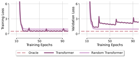
Figure 2: Poor generalization. Despite its simplicity, Transformer suffers from severe overfitting. Fixing the attention weights in Random Transformer improves the generalization, hinting at the role of attention in avoiding convergence to suboptimal local minima.

We present the validation loss for both models in Figure 2. A first surprising finding is that both transformers fail to recover $\mathbf{W}_{\mathrm{toy}}$, vividly highlighting that optimizing even such a simple architecture with a favorable design exhibits a strong lack of generalization. When fixing the self-attention matrices, the problem is alleviated to some extent although Random Transformer remains suboptimal. This observation remains consistent across various optimizers (see Appendix Figure 15), suggesting that this phenomenon is not attributable to suboptimal optimizer hyperparameters or the specific choice of the optimizer.

2.3 Transformer’s Loss Landscape

Intuition.

To develop our intuition behind the failure of transformers observed above, we plot in Figure 3(a) the attention matrices at different epochs of training. It’s observed that the attention matrix approaches an identity matrix after the very first epoch and barely changes afterward, especially with the softmax amplifying the differences in the matrix values. This pathological pattern suggests that the optimized transformer probably falls into a suboptimal local minimum, from which it struggles to exit in subsequent iterations. We hypothesize that this inability to escape from the local minimum can be explained by the sharpness of the loss landscape of the transformer, an issue that we describe and study below.

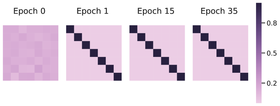
(a) Attention matrices of Transformer along the training.

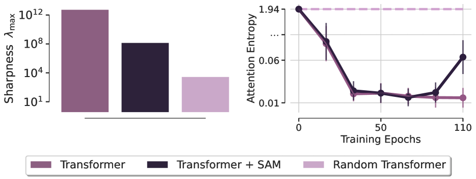
(b) Sharpness at end of training, Entropy collapse.

Figure 3: Transformer’s loss landscape analysis for linear regression. (a) The attention matrices of Transformer get stuck to identity from the first epoch. (b, left) Transformer converges to sharper minimum than Transformer+SAM with much larger $\lambda_{\mathrm{max}}$ ($\sim\times 10^{4})$, while Random Transformer has a smooth loss landscape. (b, right) Transformer suffers from entropy collapse during training confirming the high sharpness of its loss landscape.

Existing solutions.

Recent studies have demonstrated that the loss landscape of transformers is sharper compared to other residual architectures (Chen et al.,, 2022; Zhai et al.,, 2023). This may explain training instability and subpar performance of transformers, especially when trained on small-scale datasets. The sharpness of transformers was observed and quantified differently: while Chen et al., (2022) computes $\lambda_{\mathrm{max}}$, the largest eigenvalue of the loss function’s Hessian, Zhai et al., (2023) gauges the entropy of the attention matrix to demonstrate its collapse with high sharpness.

Both these metrics are evaluated, and their results are illustrated in Figure 3(b). This visualization confirms our hypothesis, revealing both detrimental phenomena at once. On the one hand, the sharpness of the transformer with fixed attention is orders of magnitude lower than the sharpness of the transformer that converges to the identity attention matrix. On the other hand, the entropy of the transformer’s attention matrix is dropping sharply along the epochs when compared to the initialization.

To identify an appropriate solution allowing a better generalization performance and training stability, we explore both remedies proposed by Chen et al., (2022) and Zhai et al., (2023). The first approach involves utilizing the recently proposed sharpness-aware minimization framework (Foret et al.,, 2021) which replaces the training objective $\mathcal{L}_{\mathrm{train}}$ of Eq. (1) by

$$\mathcal{L}_{\mathrm{train}}^{\textrm{SAM}}(\bm{\omega}) =\max_{\|\bm{\epsilon}\|<\rho}\mathcal{L}_{\mathrm{train}}(\bm{\omega}+\bm{\epsilon})\,,$$

where $\rho>0$ is an hyper-parameter (see Remark D.1 of Appendix D), and $\bm{\omega}$ are the parameters of the model. More details on SAM can be found in Appendix D.2

The second approach involves reparameterizing all weight matrices with spectral normalization and an additional learned scalar, a technique termed $\sigma$Reparam by Zhai et al., (2023). More formally, we replace each weight matrix $\mathbf{W}$ as follows

$$\widehat{\mathbf{W}}=\frac{\gamma}{\lVert\mathbf{W}\rVert_{2}}\mathbf{W},$$ (5)

where $\gamma\in\mathbb{R}$ is a learnable parameter initialized at $1$.

The results depicted in Figure 1 highlight our transformer’s successful convergence to the desired solution. Surprisingly, this is only achieved with SAM, as $\sigma$Reparam doesn’t manage to approach the optimal performance despite maximizing the entropy of the attention matrix. One can observe that the entropy of the attention obtained with SAM remains close to that of a base Transformer with a slight increase in the later stages of the training. It shows that entropy collapse as introduced in Zhai et al., (2023) may be benign in this scenario.

To understand this failure of $\sigma$Reparam, it can be useful to recall how Eq. (5) was derived. Zhai et al., (2023) departed from a tight lower bound on the attention entropy and showed that it increases exponentially fast when $\lVert\mathbf{W}_{Q}\mathbf{W}_{K}^{\top}\rVert_{2}$ is minimized (Zhai et al.,, 2023, see Theorem 3.1). Eq. (5) was proposed as a simple way to minimize this quantity. In the case of channel-wise attention, however, it can be shown that this has a detrimental effect on the rank of the attention matrix, which would consequently exclude certain features from being considered by the attention mechanism. We formalize this intuition in the following Proposition 2.3, where we consider the nuclear norm, a sum of the singular values, as a smooth proxy of the algebraic rank, which is a common practice  (Daneshmand et al.,, 2020; Dong et al.,, 2021). The proof is deferred to Appendix E.3. [Upper bound on the nuclear norm] Let $\mathbf{X}\in\mathbb{R}^{D\times L}$ be an input sequence. Assuming $\mathbf{W}_{Q}\mathbf{W}_{K}^{\top}=\mathbf{W}_{K}\mathbf{W}_{Q}^{\top}\succcurlyeq\mathbf{0}$, we have

$$\lVert\mathbf{X}\mathbf{W}_{Q}\mathbf{W}_{K}^{\top}\mathbf{X}^{\top}\rVert_{*}\leq\lVert\mathbf{W}_{Q}\mathbf{W}_{K}^{\top}\rVert_{2}\lVert\mathbf{X}\rVert_{\mathrm{F}}^{2}.$$

Note that the assumption made above holds when ${\mathbf{W}_{Q}\!=\!\mathbf{W}_{K}}$ and has been previously studied by  Kim et al., 2021a . The theorem confirms that employing $\sigma$Reparam to decrease $\lVert\mathbf{W}_{Q}\mathbf{W}_{K}^{\top}\rVert_{2}$ reduces the nuclear norm of the numerator of attention matrix defined by Eq. (4). While the direct link between matrix rank and this nuclear norm does not always hold, nuclear norm regularization is commonly used to encourage a low-rank structure in compressed sensing (Recht et al.,, 2010; Recht,, 2011; Candès and Recht,, 2012).

Although Proposition 2.3 cannot be directly applied to the attention matrix $\mathbf{A}(\mathbf{X})$, we point out that in the extreme case when $\sigma$Reparam leads to the attention scores $\mathbf{X}\mathbf{W}_{Q}\mathbf{W}_{K}^{\top}\mathbf{X}^{\top}$ to be rank-$1$ with identical rows as studied in (Anagnostidis et al.,, 2022), that the attention matrix stays rank-$1$ after application of the row-wise softmax. Thus, $\sigma$Reparam may induce a collapse of the attention rank that we empirically observe in terms of nuclear norm in Figure 7.

With these findings, we present a new simple transformer model with high performance and training stability for multivariate time series forecasting.

2.4 SAMformer: Putting It All Together

The proposed SAMformer is based on Eq. (3) with two important modifications. First, we equip it with Reversible Instance Normalization (RevIN, Kim et al., 2021b ) applied to $\mathbf{X}$ as this technique was shown to be efficient in handling the shift between the training and testing data in time series. Second, as suggested by our explorations above, we optimize the model with SAM to make it converge to flatter local minima. Overall, this gives a shallow transformer model with one encoder as represented in Figure 4.

Figure 4: SAM -former

We highlight that SAMformer keeps the channel-wise attention represented by a matrix $D\times D$ as in Eq. (3), contrary to spatial (or temporal) attention given by $L\times L$ matrix used in other models. This brings two important benefits: (i) it ensures feature permutation invariance, eliminating the need for positional encoding, commonly preceding the attention layer; (ii) it leads to a reduced time and memory complexity as $D\leq L$ in most of the real-world datasets. Our channel-wise attention examines the average impact of each feature on the others throughout all timesteps. An ablation study, detailed in Appendix C.4, validates the effectiveness of this implementation.

We are prepared to evaluate SAMformer on common multivariate time series forecasting benchmarks, demonstrating its superior performance.

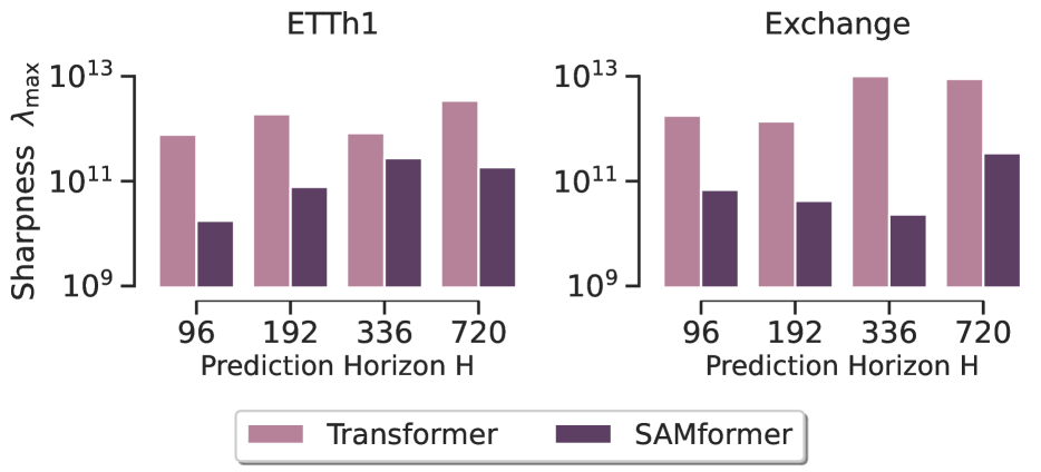
(a) Sharpness of SAMformer and Transformer.

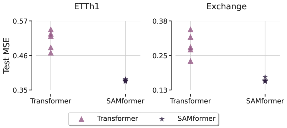
(b) Performance across runs of SAMformer and Transformer.

Figure 5: (a) SAMformer has a smoother loss landscape than Transformer. (b) SAMformer consistently generalize well for every initialization while Transformer is unstable and heavily depends on the seed.

3 Experiments

In this section, we empirically demonstrate the quantitative and qualitative superiority of SAMformer in multivariate long-term time series forecasting on common benchmarks. We show that SAMformer surpasses the current multivariate state-of-the-art TSMixer (Chen et al.,, 2023) by $14.33\%$ while having $\sim 4$ times fewer parameters. All the implementation details are provided in Appendix A.1.

Datasets.

We conduct our experiments on $8$ publicly available datasets of real-world multivariate time series, commonly used for long-term forecasting (Wu et al.,, 2021; Chen et al.,, 2023; Nie et al.,, 2023; Zeng et al.,, 2023): the $4$ Electricity Transformer Temperature datasets ETTh1, ETTh2, ETTm1 and ETTm2 Zhou et al., (2021), Electricity (UCI, nd, ), Exchange (Lai et al., 2018b, ), Traffic (California Department of Transportation, nd, ), and Weather (Max Planck Institute, nd, ) datasets. All time series are segmented with input length $L=512$, prediction horizons $H\in\{96,192,336,720\}$, and a stride of $1$, meaning that each subsequent window is shifted by one step. A more detailed description of the datasets and time series preparation can be found in Appendix A.2.

Baselines.

We compare SAMformer with several other methods including the earlier presented Transformer and the current state-of-the-art multivariate baseline, TSMixer (Chen et al.,, 2023), entirely built on MLPs. For a fair comparison, we include TSMixer’s performance when trained with SAM, along with results reported by Nie et al., (2023) and Chen et al., (2023) for other recent SOTA multivariate transformer-based models: Informer (Zhou et al.,, 2021), Autoformer (Wu et al.,, 2021), FEDformer (Zhou et al.,, 2022), Pyraformer (Liu et al.,, 2022), and LogTrans (Li et al.,, 2019). Additionally, we also incorporate RevIN into other models for a more equitable comparison between SAMformer and its competitors. Further and more detailed information on these baselines can be found in Appendix A.3.

All models are trained to minimize the MSE loss defined in Eq. (1). The average MSE on the test set, together with the standard deviation over $5$ runs with different seeds is reported. Additional details and results, including the Mean Absolute Error (MAE), can be found in Appendix B.1. Except specified otherwise, all our results are also obtained over $5$ runs with different seeds.

3.1 Main Takeaways

SAMformer improves over state-of-the-art.

The experimental results are detailed in Table 1, with a Student’s t-test analysis available in Appendix Table 6. SAMformer significantly outperforms its competitors on $\mathbf{7}$ out of $\mathbf{8}$ datasets. In particular, it improves over its best competitor TSMixer+SAM by $\mathbf{5.25\%}$, surpasses the standalone TSMixer by $\mathbf{14.33\%}$ and the best transformer-based model FEDformer by $\mathbf{12.36\%}$. In addition, it improves over Transformer by $\mathbf{16.96\%}$. For each dataset and horizon, SAMformer is ranked either first or second. Notably, SAM’s integration improves the generalization capacity of TSMixer, resulting in an average enhancement of $9.58\%$. A similar study with the MAE in Table 5 leads to the same conclusions. As TSMixer trained with SAM is the second-best baseline, it serves as a primary benchmark for further discussion in this section.

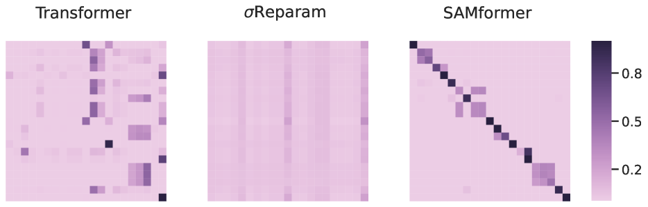
Figure 6: Attention matrices on Weather dataset. SAMformer preserves self-correlation among features while $\sigma$Reparam degrades the rank, hindering the propagation of information.

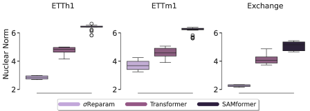
Figure 7: Nuclear norm of the attention matrix for different models: $\sigma$Reparam induces lower nuclear norm in accordance with Proposition 2.3, while SAMformer keeps the expressiveness of the attention over Transformer.

Table 1: Performance comparison between our model (SAMformer) and baselines for multivariate long-term forecasting with different horizons $H$. Results marked with ^∗ are obtained from Chen et al., (2023) and those marked with ^† are obtained from Nie et al., (2023). Transformer-based models are abbreviated by removing the “former” part of their name. We display the average test MSE with standard deviation obtained on $5$ runs with different seeds. Best results are in bold, second best are underlined.

Dataset	$H$	with SAM		without SAM
		SAMformer	TSMixer	Transformer	TSMixer	$\texttt{In}^{*}$	$\texttt{Auto}^{*}$	$\texttt{FED}^{*}$	$\texttt{Pyra}^{\dagger}$	$\texttt{LogTrans}^{\dagger}$
ETTh1	$96$	$\underline{0.381}_{\pm 0.003}$	$0.388_{\pm 0.001}$	$0.509_{\pm 0.031}$	$0.398_{\pm 0.001}$	$0.941$	$0.435$	$\mathbf{0.376}$	0$.664$	$0.878$
	$192$	$\mathbf{0.409}_{\pm 0.002}$	$\underline{0.421}_{\pm 0.002}$	$0.535_{\pm 0.043}$	$0.426_{\pm 0.003}$	$1.007$	$0.456$	$0.423$	$0.790$	$1.037$
	$336$	$\mathbf{0.423}_{\pm 0.001}$	$\underline{0.430}_{\pm 0.002}$	$0.570_{\pm 0.016}$	$0.435_{\pm 0.003}$	$1.038$	$0.486$	$0.444$	$0.891$	$1.238$
	$720$	$\mathbf{0.427}_{\pm 0.002}$	$\underline{0.440}_{\pm 0.005}$	$0.601_{\pm 0.036}$	$0.498_{\pm 0.076}$	$1.144$	$0.515$	$0.469$	$0.963$	$1.135$
ETTh2	$96$	$\mathbf{0.295}_{\pm 0.002}$	$\underline{0.305}_{\pm 0.007}$	$0.396_{\pm 0.017}$	$0.308_{\pm 0.003}$	$1.549$	$0.332$	$0.332$	$0.645$	$2.116$
	$192$	$\mathbf{0.340}_{\pm 0.002}$	$\underline{0.350}_{\pm 0.002}$	$0.413_{\pm 0.010}$	$0.352_{\pm 0.004}$	$3.792$	$0.426$	$0.407$	$0.788$	$4.315$
	$336$	$\mathbf{0.350}_{\pm 0.000}$	$\underline{0.360}_{\pm 0.002}$	$0.414_{\pm 0.002}$	$0.360_{\pm 0.002}$	$4.215$	$0.477$	$0.400$	$0.907$	$1.124$
	$720$	$\mathbf{0.391}_{\pm 0.001}$	$\underline{0.402}_{\pm 0.002}$	$0.424_{\pm 0.009}$	$0.409_{\pm 0.006}$	$3.656$	$0.453$	$0.412$	$0.963$	$3.188$
ETTm1	$96$	$0.329_{\pm 0.001}$	$\underline{0.327}_{\pm 0.002}$	$0.384_{\pm 0.022}$	$0.336_{\pm 0.004}$	$0.626$	$0.510$	$\mathbf{0.326}$	$0.543$	$0.600$
	$192$	$\mathbf{0.353}_{\pm 0.006}$	$\underline{0.356}_{\pm 0.004}$	$0.400_{\pm 0.026}$	$0.362_{\pm 0.006}$	$0.725$	$0.514$	$0.365$	$0.557$	$0.837$
	$336$	$\mathbf{0.382}_{\pm 0.001}$	$\underline{0.387}_{\pm 0.004}$	$0.461_{\pm 0.017}$	$0.391_{\pm 0.003}$	$1.005$	$0.510$	$0.392$	$0.754$	$1.124$
	$720$	$\mathbf{0.429}_{\pm 0.000}$	$\underline{0.441}_{\pm 0.002}$	$0.463_{\pm 0.046}$	$0.450_{\pm 0.006}$	$1.133$	$0.527$	$0.446$	$0.908$	$1.153$
ETTm2	$96$	$\underline{0.181}_{\pm 0.005}$	$0.190_{\pm 0.003}$	$0.200_{\pm 0.036}$	$0.211_{\pm 0.014}$	$0.355$	$0.205$	$\mathbf{0.180}$	$0.435$	$0.768$
	$192$	$\mathbf{0.233}_{\pm 0.002}$	$\underline{0.250}_{\pm 0.002}$	$0.273_{\pm 0.013}$	$0.252_{\pm 0.005}$	$0.595$	$0.278$	$0.252$	$0.730$	$0.989$
	$336$	$\mathbf{0.285}_{\pm 0.001}$	$\underline{0.301}_{\pm 0.003}$	$0.310_{\pm 0.022}$	$0.303_{\pm 0.004}$	$1.270$	$0.343$	$0.324$	$1.201$	$1.334$
	$720$	$\mathbf{0.375}_{\pm 0.001}$	$\underline{0.389}_{\pm 0.002}$	$0.426_{\pm 0.025}$	$0.390_{\pm 0.003}$	$3.001$	$0.414$	$0.410$	$3.625$	$3.048$
Electricity	$96$	$\mathbf{0.155}_{\pm 0.002}$	$\underline{0.171}_{\pm 0.001}$	$0.182_{\pm 0.006}$	$0.173_{\pm 0.004}$	$0.304$	$0.196$	$0.186$	$0.386$	$0.258$
	$192$	$\mathbf{0.168}_{\pm 0.001}$	$\underline{0.191}_{\pm 0.010}$	$0.202_{\pm 0.041}$	$0.204_{\pm 0.027}$	$0.327$	$0.211$	$0.197$	$0.386$	$0.266$
	$336$	$\mathbf{0.183}_{\pm 0.000}$	$\underline{0.198}_{\pm 0.006}$	$0.212_{\pm 0.017}$	$0.217_{\pm 0.018}$	$0.333$	$0.214$	$0.213$	$0.378$	$0.280$
	$720$	$\mathbf{0.219}_{\pm 0.000}$	$\underline{0.230}_{\pm 0.005}$	$0.238_{\pm 0.016}$	$0.242_{\pm 0.015}$	$0.351$	$0.236$	$0.233$	$0.376$	$0.283$
Exchange	$96$	$\underline{0.161}_{\pm 0.007}$	${0.233}_{\pm 0.016}$	$0.292_{\pm 0.045}$	$0.343_{\pm 0.082}$	$0.847$	$0.197$	$\mathbf{0.139}$	-	$0.968$
	$192$	$\mathbf{0.246}_{\pm 0.009}$	$\underline{0.342}_{\pm 0.031}$	$0.372_{\pm 0.035}$	$0.342_{\pm 0.031}$	$1.204$	$0.300$	$0.256$	-	$1.040$
	$336$	$\mathbf{0.368}_{\pm 0.006}$	$\underline{0.474}_{\pm 0.014}$	$0.494_{\pm 0.033}$	$0.484_{\pm 0.062}$	$1.672$	$0.509$	$0.426$	-	$1.659$
	$720$	$\mathbf{1.003}_{\pm 0.018}$	$\underline{1.078}_{\pm 0.179}$	$1.323_{\pm 0.192}$	$1.204_{\pm 0.028}$	$2.478$	$1.447$	$1.090$	-	$1.941$
Traffic	$96$	$\mathbf{0.407}_{\pm 0.001}$	$\underline{0.409}_{\pm 0.016}$	$0.420_{\pm 0.041}$	$0.409_{\pm 0.016}$	$0.733$	$0.597$	$0.576$	$2.085$	$0.684$
	$192$	$\mathbf{0.415}_{\pm 0.005}$	$\underline{0.433}_{\pm 0.009}$	$0.441_{\pm 0.039}$	$0.637_{\pm 0.444}$	$0.777$	$0.607$	$0.610$	$0.867$	$0.685$
	$336$	$\mathbf{0.421}_{\pm 0.001}$	$\underline{0.424}_{\pm 0.000}$	$0.501_{\pm 0.154}$	$0.747_{\pm 0.277}$	$0.776$	$0.623$	$0.608$	$0.869$	$0.734$
	$720$	$\mathbf{0.456}_{\pm 0.003}$	$\underline{0.488}_{\pm 0.028}$	$0.468_{\pm 0.021}$	$0.688_{\pm 0.287}$	$0.827$	$0.639$	$0.621$	$0.881$	$0.717$
Weather	$96$	$\underline{0.197}_{\pm 0.001}$	$\mathbf{0.189}_{\pm 0.003}$	$0.227_{\pm 0.012}$	$0.214_{\pm 0.004}$	$0.354$	$0.249$	$0.238$	$0.896$	$0.458$
	$192$	$\underline{0.235}_{\pm 0.000}$	$\mathbf{0.228}_{\pm 0.004}$	$0.256_{\pm 0.018}$	$0.231_{\pm 0.003}$	$0.419$	$0.325$	$0.275$	$0.622$	$0.658$
	$336$	$\underline{0.276}_{\pm 0.001}$	$\mathbf{0.271}_{\pm 0.001}$	$0.278_{\pm 0.001}$	$0.279_{\pm 0.007}$	$0.583$	$0.351$	$0.339$	$0.739$	$0.797$
	$720$	$\underline{0.334}_{\pm 0.000}$	$\mathbf{0.331}_{\pm 0.001}$	$0.353_{\pm 0.002}$	$0.343_{\pm 0.024}$	$0.916$	$0.415$	$0.389$	$1.004$	$0.869$
Overall MSE improvement			$\mathbf{5.25\%}$	$\mathbf{16.96\%}$	$\mathbf{14.33\%}$	$\mathbf{72.20\%}$	$\mathbf{22.65\%}$	$\mathbf{12.36\%}$	$\mathbf{61.88\%}$	$\mathbf{70.88\%}$

Smoother loss landscape.

The introduction of SAM in the training of SAMformer makes its loss smoother than that of Transformer. We illustrate this in Figure 5(a) by comparing the values of $\lambda_{\mathrm{max}}$ for Transformer and SAMformer after training on ETTh1 and Exchange. Our observations reveal that Transformer exhibits considerably higher sharpness, while SAMformer has a desired behavior with a loss landscape sharpness that is an order of magnitude smaller.

Improved robustness.

SAMformer demonstrates robustness against random initialization. Figure 5(b) illustrates the test MSE distribution of SAMformer and Transformer across $5$ different seeds on ETTh1 and Exchange with a prediction horizon of $H=96$. SAMformer consistently maintains performance stability across different seed choices, while Transformer exhibits significant variance and, thus, a high dependency on weight initialization. This observation holds across all datasets and prediction horizons as shown in Appendix B.4.

3.2 Qualitative Benefits of Our Approach

Computational efficiency.

SAMformer is computationally more efficient than TSMixer and usual transformer-based approaches, benefiting from a shallow lightweight implementation, i.e., a single layer with one attention head. The number of parameters of SAMformer and TSMixer is detailed in Appendix Table 7. We observe that, on average, SAMformer has $\sim 4$ times fewer parameters than TSMixer, which makes this approach even more remarkable. Importantly, TSMixer itself is recognized as a computationally efficient architecture compared to the transformer-based baselines (Chen et al.,, 2023, Table 6).

Fewer hyperparameters and versatility.

SAMformer requires minimal hyperparameters tuning, contrary to other baselines, including TSMixer and FEDformer. In particular, SAMformer’s architecture remains the same for all our experiments (see Appendix A.1 for details), while TSMixer varies in terms of the number of residual blocks and feature embedding dimensions, depending on the dataset. This versatility also comes with better robustness to the prediction horizon $H$. In Appendix C.1 Figure 13, we display the evolution forecasting accuracy on all datasets for $H\in\{96,192,336,720\}$ for SAMformer and TSMixer (trained with SAM). We observe that SAMformer consistently outperforms its best competitor TSMixer (trained with SAM) for all horizons.

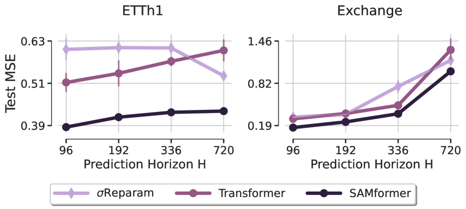
(a) Comparison of Transformer, $\sigma$Reparam and SAMformer.

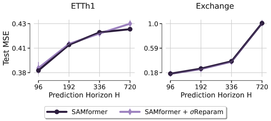
(b) Comparison of SAMformer and SAMformer+$\sigma$Reparam.

Figure 8: Suboptimality of $\sigma$Reparam. (a) $\sigma$Reparam alone does not bring improvement on Transformer and is clearly outperformed by SAMformer. Combining $\sigma$Reparam with SAMformer does not bring significant improvement but heavily increases the training time (see Figure 11).

Better attention.

We display the attention matrices after training on Weather with the prediction horizon $H=96$ for Transformer, SAMformer and Transformer + $\sigma$Reparam in Figure 6. We note that Transformer excludes self-correlation between features, having low values on the diagonal, while SAMformer strongly promotes them. This pattern is reminiscent of He et al., (2023) and Trockman and Kolter, (2023): both works demonstrated the importance of diagonal patterns in attention matrices for signal propagation in transformers used in NLP and computer vision. Our experiments reveal that these insights also apply to time-series forecasting. Note that freezing the attention to $\mathbf{A}(\mathbf{X})=\mathbf{I}_{D}$ is largely outperformed by SAMformer as shown in Table 9, Appendix C.4, which confirms the importance of learnable attention. The attention matrix given by $\sigma$Reparam at Figure 6 has almost equal rows, leading to rank collapse. In Figure 7, we display the distributions of nuclear norms of attention matrices after training Transformer, SAMformer and $\sigma$Reparam. We observe that $\sigma$Reparam heavily penalizes the nuclear norms of the attention matrix, which is coherent with Proposition 2.3. In contrast, SAMformer maintains it above Transformer, thus improving the expressiveness of attention.

3.3 Ablation Study and Sensitivity Analysis

Choices of implementation.

We empirically compared our architecture, which is channel-wise attention (Eq. (3)), with temporal-wise attention. Table 8 of Appendix C.4 shows the superiority of our approach in the considered setting. We conducted our experiments with Adam (Kingma and Ba,, 2015), the de-facto optimizers for transformers (Ahn et al.,, 2023; Pan and Li,, 2022; Zhou et al.,, 2022, 2021; Chen et al.,, 2022). We provide an in-depth ablation study in Appendix C.3 that motivates this choice. As expected (Ahn et al.,, 2023; Liu et al.,, 2020; Pan and Li,, 2022; Zhang et al.,, 2020), SGD (Nesterov,, 1983) fails to converge and AdamW (Loshchilov and Hutter,, 2019) leads to similar performance but is very sensitive to the choice of the weight decay strength.

Sensitivity to the neighborhood size $\rho$.

The test MSE of SAMformer and TSMixer is depicted in Figure 14 of Appendix C.2 as a function of the neighborhood size $\rho$. It appears that TSMixer, with its quasi-linear architecture, exhibits less sensitivity to $\rho$ compared to SAMformer. This behavior is consistent with the understanding that, in linear models, the sharpness does not change with respect to $\rho$, given the constant nature of the loss function’s Hessian. Consequently, TSMixer benefits less from changes in $\rho$ than SAMformer. Our observations consistently show that a sufficiently large $\rho$, generally above $0.7$ enables SAMformer to achieve lower MSE than TSMixer.

SAM vs $\sigma$Reparam.

We mentioned previously that $\sigma$Reparam doesn’t improve the performance of a transformer on a simple toy example, although it makes it comparable to the performance of a transformer with fixed random attention. To further show that $\sigma$Reparam doesn’t provide an improvement on real-world datasets, we show in Figure 8(a) that on ETTh1 and Exchange, $\sigma$Reparam alone fails to match SAMformer’s improvements, even underperforming Transformer in some cases. A potential improvement may come from combining SAM and $\sigma$Reparam to smooth a rather sparse matrix obtained with SAM. However, as Figure 8(b) illustrates, this combination does not surpass the performance of using SAM alone. Furthermore, combining SAM and $\sigma$Reparam significantly increases training time and memory usage, especially for larger datasets and longer horizons (see Appendix Figure 11), indicating its inefficiency as a method.

4 Discussion and Future Work

In this work, we demonstrated how simple transformers can reclaim their place as state-of-the-art models in long-term multivariate series forecasting from their MLP-based competitors. Rather than concentrating on new architectures and attention mechanisms, we analyzed the current pitfalls of transformers in this task and addressed them by carefully designing an appropriate training strategy. Our findings suggest that even a simple shallow transformer has a very sharp loss landscape which makes it converge to poor local minima. We analyzed popular solutions proposed in the literature to address this issue and showed which of them work or fail. Our proposed SAMformer, optimized with sharpness-aware minimization, leads to a substantial performance gain compared to the existing forecasting baselines and benefits from a high versatility and robustness across datasets and prediction horizons. Finally, we also showed that channel-wise attention in time series forecasting can be more efficient – both computationally and performance-wise – than temporal attention commonly used previously. We believe that this surprising finding may spur many further works building on top of our simple architecture to improve it even further.

 

Unlocking the Potential of Transformers: Supplementary Materials

 

Roadmap.

In this appendix, we provide the detailed experimental setup in Section A, additional experiments in Section B, and a thorough ablation study and sensitivity analysis in Section C. Additional background knowledge is available in Section D and proofs of the main theoretical results are provided in Section E. We display below the corresponding table of contents.

Table of Contents

1. 1 Introduction
2. 2 Proposed Approach
   1. 2.1 Problem Setup
   2. 2.2 Motivational Example
   3. 2.3 Transformer’s Loss Landscape
   4. 2.4 SAMformer: Putting It All Together
3. 3 Experiments
   1. 3.1 Main Takeaways
   2. 3.2 Qualitative Benefits of Our Approach
   3. 3.3 Ablation Study and Sensitivity Analysis
4. 4 Discussion and Future Work
5. A Experimental Setup
   1. A.1 Architecture and Training Parameters
   2. A.2 Datasets
   3. A.3 More Details on the Baselines
6. B Additional Experiments
   1. B.1 MAE Results
   2. B.2 Significance Test for SAMformer and TSMixer with SAM
   3. B.3 Computational Efficiency of SAMformer
   4. B.4 Strong Generalization Regardless of the Initialization
   5. B.5 Faithful Signal Propagation
7. C Ablation Study and Sensitivity Analysis
   1. C.1 Sensitivity to the Prediction Horizon $H$.
   2. C.2 Sensitivity to the Neighborhood Size $\rho$.
   3. C.3 Sensitivity to the Change of the Optimizer.
   4. C.4 Ablation on the Implementation.
8. D Additional Background
   1. D.1 Reversible Instance Normalization: RevIN
   2. D.2 Sharpness-aware minimization (SAM)
9. E Proofs
   1. E.1 Notations
   2. E.2 Proof of Proposition 2.2
   3. E.3 Proof of Proposition
   4. E.4 Proof of Proposition 9
   5. E.5 Matrix formulation of $\mathbf{\hat{Y}}$ in Eq. (11)

Appendix A Experimental Setup

A.1 Architecture and Training Parameters

Architecture.

We follow Chen et al., (2023); Nie et al., (2023), and to ensure a fair comparison of baselines, we apply the reversible instance normalization (RevIN) of Kim et al., 2021b (see Appendix D.1 for more details). The network used in SAMformer and Transformer is a simplified one-layer transformer with one head of attention and without feed-forward. Its neural network function follows Eq. (3), while RevIN normalization and denormalization are applied respectively before and after the neural network function, see Figure 4. We display the inference step of SAMformer in great details in Algorithm 1. For the sake of clarity, we describe the application of the neural network function sequentially on each element of the batches but in practice, the operations are parallelized and performed batch per batch. For SAMformer and Transformer, the dimension of the model is $d_{\mathrm{m}}=16$ and remains the same in all our experiments. For TSMixer, we used the official implementation than can be found on Github. For all of our experiments, we train our baselines (SAMformer, Transformer, TSMixer with SAM, TSMixer without SAM) with the Adam optimizer (Kingma and Ba,, 2015), a batch size of $32$, a cosine annealing scheduler (Loshchilov and Hutter,, 2017) and the learning rates summarized in Table 2.

Training parameters.

For SAMformer and TSMixer trained with SAM, the values of neighborhood size $\rho^{*}$ used are reported in Table 3. The training/validation/test split is $12/4/4$ months on the ETT datasets and $70\%/20\%/10\%$ on the other datasets. We use a look-back window $L=512$ and use a sliding window with stride $1$ to create the sequences. The training loss is the MSE on the multivariate time series (Eq. (1)). Training is performed during $300$ epochs and we use early stopping with a patience of $5$ epochs. For each dataset, baselines, and prediction horizon $H\in\{96,192,336,720\}$, each experiment is run $5$ times with different seeds, and we display the average and the standard deviation of the test MSE and MAE over the $5$ trials.

Table 2: Learning rates used in our experiments.

Dataset	ETTh1/ETTh2	ETTm1/ETTm2	Electricity	Exchange	Traffic	Weather
Learning rate	$0.01$	$0.01$	$0.0001$	$0.001$	$0.0001$	$0.0001$

Table 3: Neighborhood size $\rho^{*}$ at which SAMformer and TSMixer achieve their best performance on the benchmarks described in Table 4.

H	Model	ETTh1	ETTh2	ETTm1	ETTm2	Electricity	Exchange	Traffic	Weather
96	SAMformer	0.5	0.5	0.6	0.2	0.5	0.7	0.8	0.4
	TSMixer	1.0	0.9	1.0	1.0	0.9	1.0	0.0	0.5
192	SAMformer	0.6	0.8	0.9	0.9	0.6	0.8	0.1	0.4
	TSMixer	0.7	0.1	0.6	1.0	1.0	0.0	0.9	0.4
336	SAMformer	0.9	0.6	0.9	0.8	0.5	0.5	0.5	0.6
	TSMixer	0.7	0.0	0.7	1.0	0.4	1.0	0.6	0.6
720	SAMformer	0.9	0.8	0.9	0.9	1.0	0.9	0.7	0.5
	TSMixer	0.3	0.4	0.5	1.0	0.9	0.1	0.9	0.3

A.2 Datasets

We conduct our experiments on $8$ publicly available datasets of real-world time series, widely used for multivariate long-term forecasting (Wu et al.,, 2021; Chen et al.,, 2023; Nie et al.,, 2023). The $4$ Electricity Transformer Temperature datasets ETTm1, ETTm2, ETTh1, and ETTh2 (Zhou et al.,, 2021) contain the time series collected by electricity transformers from July 2016 to July 2018. Whenever possible, we refer to this set of $4$ datasets as ETT. Electricity (UCI, nd, ) contains the time series of electricity consumption from $321$ clients from 2012 to 2014. Exchange (Lai et al., 2018b, ) contains the time series of daily exchange rates between $8$ countries from 1990 to 2016. Traffic (California Department of Transportation, nd, ) contains the time series of road occupancy rates captured by $862$ sensors from January 2015 to December 2016. Last but not least, Weather (Max Planck Institute, nd, ) contains the time series of meteorological information recorded by 21 weather indicators in 2020. It should be noted that Electricity, Traffic, and Weather are large-scale datasets. The ETT datasets can be downloaded here while the $4$ other datasets can be downloaded here. Table 4 sums up the characteristics of the datasets used in our experiments.

Table 4: Characteristics of the multivariate time series datasets used in our experiments.

Dataset	ETTh1/ETTh2	ETTm1/ETTm2	Electricity	Exchange	Traffic	Weather
# features	$7$	$7$	$321$	$9$	$862$	$21$
# time steps	$17420$	$699680$	$26304$	$7588$	$17544$	$52696$
Granularity	1 hour	15 minutes	1 hour	1 day	1 hour	10 minutes

Parameters: Batch size $bs$, input length $L$, prediction horizon $H$, dimension of the model $d_{\mathrm{m}}$.

Network trainable parameters: $\mathbf{W}_{Q}\in\mathbb{R}^{L\times d_{\mathrm{m}}},\mathbf{W}_{K}\in\mathbb{R}^{L\times d_{\mathrm{m}}}$, $\mathbf{W}_{V}\in\mathbb{R}^{L\times d_{\mathrm{m}}}$, $\mathbf{W}_{O}\in\mathbb{R}^{d_{\mathrm{m}}\times L}$, $\mathbf{W}\in\mathbb{R}^{L\times H}$.

RevIN trainable parameters: $\bm{\beta},\bm{\gamma}$.

Input: Batch of $bs$ input sequences $\mathbf{X}\in\mathbb{R}^{D\times L}$ arranged in a tensor $\mathbf{B}_{\mathrm{in}}$ of dimension $bs\times L\times D$.

RevIN normalization: $\mathbf{X}\leftarrow\tilde{\mathbf{X}}$ following Eq. (7). The output is a tensor $\tilde{\mathbf{B}}_{\mathrm{in}}$ of dimension $bs\times L\times D$.

Transposition of the batch: $\tilde{\mathbf{B}}_{\mathrm{in}}$ is reshaped in dimension $bs\times D\times L$.

Applying the neural network of Eq. (3):

for each $\tilde{\mathbf{X}}\in\tilde{\mathbf{B}}_{\mathrm{in}}$ do

       1. Attention layer

       Rescale the input with the attention matrix (Eq. (4)).

       The output $\mathbf{A}(\tilde{\mathbf{X}})\tilde{\mathbf{X}}\mathbf{W}_{V}\mathbf{W}_{O}$ is of dimension $D\times L$

       2. Skip connection

       Sum the input $\tilde{\mathbf{X}}$ and the output of the attention layer.

       The output $\tilde{\mathbf{X}}+\mathbf{A}(\tilde{\mathbf{X}})\tilde{\mathbf{X}}\mathbf{W}_{V}\mathbf{W}_{O}$ is of dimension $D\times L$.

       3. Linear layer

       Apply a linear layer on the output of the skip connection.

       The output $\tilde{\mathbf{Y}}=\left[\tilde{\mathbf{X}}+\mathbf{A}(\tilde{\mathbf{X}})\tilde{\mathbf{X}}\mathbf{W}_{V}\mathbf{W}_{O}\right]\mathbf{W}$ is of dimension $D\times H$.

       Unnormalized predictions are arranged in a tensor $\tilde{\mathbf{B}}_{\mathrm{out}}$ of dimension $bs\times D\times H$.

      

end for

Transposition of the batch: $\tilde{\mathbf{B}}_{\mathrm{out}}$ is reshaped in dimension $bs\times H\times D$.

RevIN denormalization: $\tilde{\mathbf{Y}}\leftarrow\hat{\mathbf{Y}}$ following Eq. (8).

Output: Batch of $bs$ prediction sequences $\hat{\mathbf{Y}}\in\mathbb{R}^{D\times H}$ arranged in a tensor $\hat{\mathbf{B}}_{\mathrm{out}}$ of dimension $bs\times H\times D$.

Algorithm 1 Architecture of the network used in SAMformer and Transformer

A.3 More Details on the Baselines

As stated above, we conducted all our experiments with a look-back window $L=512$ and prediction horizons $H\in\{96,192,336,720\}$. Results reported in Table 1 from SAMformer, TSMixer, and Transformer come from our own experiments, conducted over $5$ runs with $5$ different seeds. The reader might notice that the results of TSMixer without SAM slightly differ from the ones reported in the original paper (Chen et al.,, 2023). It comes from the fact that the authors reported results from a single seed, while we report average performance with standard deviation on multiple runs for a better comparison of methods. We perform a Student’s t-test in Table 6 for a more thorough comparison of SAMformer and TSMixer with SAM. It should be noted that, unlike our competitors including TSMixer, the architecture of SAMformer remains the same for all the datasets. This highlights the robustness of our method and its advantage as no heavy hyperparameter tuning is required. For a fair comparison of models, we also report results from other baselines in the literature that we did not run ourselves. For Informer Zhou et al., (2021), Autoformer (Wu et al.,, 2021), and Fedformer (Zhou et al.,, 2022), the results on all datasets, except Exchange, are reported from Chen et al., (2023). Similarly, for Pyraformer (Liu et al.,, 2022) and LogTrans (Li et al.,, 2019), results on all datasets except Exchange are reported from Nie et al., (2023). It is important to note that these two baselines were not implemented with RevIN (Kim et al., 2021b, ). Results on the Exchange dataset for those $5$ baselines come from the original corresponding papers and hence refer to the models without RevIN. This approach ensures a comprehensive and comparative analysis across various established models in multivariate long-term time series forecasting.

Appendix B Additional Experiments

In this section, we provide additional experiments to showcase, quantitatively and qualitatively, the superiority of our approach.

B.1 MAE Results

In this section, we provide the performance comparison of the different baselines with the Mean Absolute Error (MAE). We display the results in Table 5. The conclusion are similar to the one made in the main paper and confirms the superiority of SAMformer.

Table 5: Performance comparison between our model (SAMformer) and baselines for multivariate long-term forecasting with different horizons $H$. Results marked with ^∗ are obtained from Chen et al., (2023) and those marked with ^† are obtained from Nie et al., (2023). Transformer-based models are abbreviated by removing the “former” part of their name. We display the average test MAE with standard deviation obtained on $5$ runs with different seeds. Best results are in bold, second best are underlined.

Dataset	$H$	with SAM		without SAM
		SAMformer	TSMixer	Transformer	TSMixer	$\texttt{In}^{*}$	$\texttt{Auto}^{*}$	$\texttt{FED}^{*}$	$\texttt{Pyra}^{\dagger}$	$\texttt{LogTrans}^{\dagger}$
ETTh1	$96$	$\mathbf{0.402}_{\pm 0.001}$	$\underline{0.408}_{\pm 0.001}$	$0.619_{\pm 0.203}$	$0.414_{\pm 0.004}$	0.769	0.446	$0.415$	0.612	0.740
	$192$	$\mathbf{0.418}_{\pm 0.001}$	$\underline{0.426}_{\pm 0.002}$	$0.513_{\pm 0.024}$	$0.428_{\pm 0.001}$	0.786	0.457	0.446	0.681	0.824
	$336$	$\mathbf{0.425}_{\pm 0.000}$	$\underline{0.434}_{\pm 0.001}$	$0.529_{\pm 0.008}$	$\underline{0.434}_{\pm 0.001}$	0.784	0.487	0.462	0.738	0.932
	$720$	$\mathbf{0.449}_{\pm 0.002}$	$\underline{0.459}_{\pm 0.004}$	$0.553_{\pm 0.021}$	$0.506_{\pm 0.064}$	0.857	0.517	0.492	0.782	0.852
ETTh2	$96$	$\mathbf{0.358}_{\pm 0.002}$	$\underline{0.367}_{\pm 0.002}$	$0.416_{\pm 0.025}$	$\underline{0.367}_{\pm 0.003}$	0.952	0.368	0.374	0.597	1.197
	$192$	$\mathbf{0.386}_{\pm 0.003}$	$\underline{0.393}_{\pm 0.001}$	$0.435_{\pm 0.019}$	$0.395_{\pm 0.003}$	1.542	0.434	0.446	0.683	1.635
	$336$	$\mathbf{0.395}_{\pm 0.002}$	$\underline{0.404}_{\pm 0.004}$	$0.434_{\pm 0.014}$	$\underline{0.404}_{\pm 0.002}$	1.642	0.479	0.447	0.747	1.604
	$720$	$\mathbf{0.428}_{\pm 0.001}$	$\underline{0.435}_{\pm 0.002}$	$0.448_{\pm 0.006}$	$0.441_{\pm 0.005}$	1.619	0.490	0.469	0.783	1.540
ETTm1	$96$	$\mathbf{0.363}_{\pm 0.001}$	$\mathbf{0.363}_{\pm 0.001}$	$0.395_{\pm 0.024}$	$0.371_{\pm 0.002}$	0.560	0.492	$0.390$	0.510	0.546
	$192$	$\mathbf{0.378}_{\pm 0.003}$	$\underline{0.381}_{\pm 0.002}$	$0.414_{\pm 0.027}$	$0.384_{\pm 0.003}$	0.619	0.495	0.415	0.537	0.700
	$336$	$\mathbf{0.394}_{\pm 0.001}$	$\underline{0.397}_{\pm 0.002}$	$0.445_{\pm 0.009}$	$0.399_{\pm 0.003}$	0.741	0.492	0.425	0.655	0.832
	$720$	$\mathbf{0.418}_{\pm 0.000}$	$\underline{0.425}_{\pm 0.001}$	$0.456_{\pm 0.035}$	$0.429_{\pm 0.002}$	0.845	0.493	0.458	0.724	0.820
ETTm2	$96$	$\underline{0.274}_{\pm 0.010}$	$0.284_{\pm 0.004}$	$0.290_{\pm 0.026}$	$0.302_{\pm 0.013}$	0.462	0.293	$\mathbf{0.271}$	0.507	0.642
	$192$	$\mathbf{0.306}_{\pm 0.001}$	$0.320_{\pm 0.001}$	$0.347_{\pm 0.025}$	$0.323_{\pm 0.005}$	0.586	0.336	0.318	0.673	0.757
	$336$	$\mathbf{0.338}_{\pm 0.001}$	$\underline{0.350}_{\pm 0.001}$	$0.360_{\pm 0.017}$	$0.352_{\pm 0.003}$	0.871	0.379	0.364	0.845	0.872
	$720$	$\mathbf{0.390}_{\pm 0.001}$	$\underline{0.402}_{\pm 0.002}$	$0.424_{\pm 0.014}$	$\underline{0.402}_{\pm 0.003}$	1.267	0.419	0.420	1.451	1.328
Electricity	$96$	$\mathbf{0.252}_{\pm 0.002}$	$\underline{0.273}_{\pm 0.001}$	$0.288_{\pm 0.013}$	$0.277_{\pm 0.003}$	0.393	0.313	0.302	0.449	0.357
	$192$	$\mathbf{0.263}_{\pm 0.001}$	$\underline{0.292}_{\pm 0.011}$	$0.304_{\pm 0.033}$	$0.304_{\pm 0.027}$	0.417	0.324	0.311	0.443	0.368
	$336$	$\mathbf{0.277}_{\pm 0.000}$	$\underline{0.297}_{\pm 0.007}$	$0.315_{\pm 0.018}$	$0.317_{\pm 0.018}$	0.422	0.327	0.328	0.443	0.380
	$720$	$\mathbf{0.306}_{\pm 0.000}$	$\underline{0.321}_{\pm 0.006}$	$0.330_{\pm 0.014}$	$0.333_{\pm 0.015}$	0.427	0.342	0.344	0.445	0.376
Exchange	$96$	$\underline{0.306}_{\pm 0.006}$	${0.363}_{\pm 0.013}$	$0.369_{\pm 0.049}$	$0.436_{\pm 0.054}$	0.752	0.323	$\mathbf{0.276}$	-	0.812
	$192$	$0.371_{\pm 0.008}$	$0.437_{\pm 0.021}$	$0.416_{\pm 0.041}$	$0.437_{\pm 0.021}$	0.895	$\mathbf{0.369}$	$\mathbf{0.369}$	-	0.851
	$336$	$\mathbf{0.453}_{\pm 0.004}$	$0.515_{\pm 0.006}$	$0.491_{\pm 0.036}$	$0.523_{\pm 0.029}$	1.036	0.524	0.464	-	1.081
	$720$	$\mathbf{0.750}_{\pm 0.006}$	$\underline{0.777}_{\pm 0.064}$	$0.823_{\pm 0.040}$	$0.818_{\pm 0.007}$	1.310	0.941	0.800	-	1.127
Traffic	$96$	$\mathbf{0.292}_{\pm 0.001}$	$\underline{0.300}_{\pm 0.020}$	$0.306_{\pm 0.033}$	$\underline{0.300}_{\pm 0.020}$	0.410	0.371	0.359	0.468	0.384
	$192$	$\mathbf{0.294}_{\pm 0.005}$	$\underline{0.317}_{\pm 0.012}$	$0.321_{\pm 0.034}$	$0.419_{\pm 0.218}$	0.435	0.382	0.380	0.467	0.390
	$336$	$\mathbf{0.292}_{\pm 0.000}$	$\underline{0.299}_{\pm 0.000}$	$0.348_{\pm 0.093}$	$0.501_{\pm 0.163}$	0.434	0.387	0.375	0.469	0.408
	$720$	$\mathbf{0.311}_{\pm 0.003}$	$0.344_{\pm 0.026}$	$\underline{0.325}_{\pm 0.023}$	$0.458_{\pm 0.159}$	0.466	0.395	0.375	0.473	0.396
Weather	$96$	$\underline{0.249}_{\pm 0.001}$	$\mathbf{0.242}_{\pm 0.002}$	$0.281_{\pm 0.018}$	$0.271_{\pm 0.009}$	0.405	0.329	0.314	0.556	0.490
	$192$	$0.277_{\pm 0.000}$	$\mathbf{0.272}_{\pm 0.003}$	$0.302_{\pm 0.020}$	$\underline{0.275}_{\pm 0.003}$	0.434	0.370	0.329	0.624	0.589
	$336$	$\underline{0.304}_{\pm 0.001}$	$\mathbf{0.299}_{\pm 0.001}$	$0.310_{\pm 0.012}$	$0.307_{\pm 0.009}$	0.543	0.391	0.377	0.753	0.652
	$720$	$\underline{0.342}_{\pm 0.000}$	$\mathbf{0.341}_{\pm 0.002}$	$0.363_{\pm 0.002}$	$0.351_{\pm 0.021}$	0.705	0.426	0.409	0.934	0.675
Overall MAE improvement			$\mathbf{3.99\%}$	$\mathbf{11.63\%}$	$\mathbf{9.60\%}$	$\mathbf{53.00\%}$	$\mathbf{15.67\%}$	$\mathbf{9.93\%}$	$\mathbf{44.44\%}$	$\mathbf{54.44\%}$

B.2 Significance Test for SAMformer and TSMixer with SAM

In this section, we perform a Student t-test between SAMformer and TSMixer trained with SAM. It should be noted that TSMixer with SAM significantly outperforms vanilla TSMixer. We report the results in Table 6. We observe that the SAMformer significantly improves upon TSMixer trained with SAM on $7$ out of $8$ datasets.

Table 6: Significance test with Student’s t-test and performance comparison between SAMformer and TSMixer trained with SAM across various datasets and prediction horizons. We display the average and standard deviation of the test MSE obtained on $5$ runs ($\mathrm{mean}_{\pm\mathrm{std}}$). The performance of the best model is in bold when the improvement is statistically significant at the level $0.05$ ($\text{p-value}<0.05$).

H	Model	ETTh1	ETTh2	ETTm1	ETTm2	Electricity	Exchange	Traffic	Weather
96	SAMformer	$\textbf{0.381}_{\pm 0.003}$	$\textbf{0.295}_{\pm 0.002}$	$0.329_{\pm 0.001}$	$\textbf{0.181}_{\pm 0.005}$	$\textbf{0.155}_{\pm 0.002}$	$\textbf{0.161}_{\pm 0.007}$	$0.407_{\pm 0.001}$	$0.197_{\pm 0.001}$
	TSMixer	$0.388_{\pm 0.001}$	$0.305_{\pm 0.007}$	$0.327_{\pm 0.002}$	$0.190_{\pm 0.003}$	$0.171_{\pm 0.001}$	$0.233_{\pm 0.016}$	$0.409_{\pm 0.016}$	$\textbf{0.189}_{\pm 0.003}$
192	SAMformer	$\textbf{0.409}_{\pm 0.002}$	$\textbf{0.340}_{\pm 0.002}$	$0.353_{\pm 0.006}$	$\textbf{0.233}_{\pm 0.002}$	$\textbf{0.168}_{\pm 0.001}$	$\textbf{0.246}_{\pm 0.009}$	$\textbf{0.415}_{\pm 0.005}$	$0.235_{\pm 0.000}$
	TSMixer	$0.421_{\pm 0.002}$	$0.350_{\pm 0.002}$	$0.356_{\pm 0.004}$	$0.250_{\pm 0.002}$	$0.191_{\pm 0.010}$	$0.342_{\pm 0.031}$	$0.433_{\pm 0.009}$	$\textbf{0.228}_{\pm 0.004}$
336	SAMformer	$\textbf{0.423}_{\pm 0.001}$	$\textbf{0.350}_{\pm 0.000}$	$\textbf{0.382}_{\pm 0.001}$	$\textbf{0.285}_{\pm 0.001}$	$\textbf{0.183}_{\pm 0.000}$	$\textbf{0.368}_{\pm 0.006}$	$\textbf{0.421}_{\pm 0.001}$	$0.276_{\pm 0.001}$
	TSMixer	$0.430_{\pm 0.002}$	$0.360_{\pm 0.002}$	$0.387_{\pm 0.004}$	$0.301_{\pm 0.003}$	$0.198_{\pm 0.006}$	$0.474_{\pm 0.014}$	$0.424_{\pm 0.000}$	$\textbf{0.271}_{\pm 0.001}$
720	SAMformer	$\textbf{0.427}_{\pm 0.002}$	$\textbf{0.391}_{\pm 0.001}$	$\textbf{0.429}_{\pm 0.000}$	$\textbf{0.375}_{\pm 0.001}$	$\textbf{0.219}_{\pm 0.000}$	$1.003_{\pm 0.018}$	$\textbf{0.456}_{\pm 0.003}$	$0.334_{\pm 0.000}$
	TSMixer	$0.440_{\pm 0.005}$	$0.402_{\pm 0.002}$	$0.441_{\pm 0.002}$	$0.389_{\pm 0.002}$	$0.230_{\pm 0.005}$	$1.078_{\pm 0.179}$	$0.488_{\pm 0.028}$	$\textbf{0.331}_{\pm 0.001}$

B.3 Computational Efficiency of SAMformer

In this section, we showcase the computational efficiency of our approach. We compare in Table 7 the number of parameters of SAMformer and TSMixer on the several benchmarks used in our experiments. We also display the ratio between the number of parameters of TSMixer and the number of parameters of SAMformer. Overall, SAMformer has $\sim 4$ times fewer parameters than TSMixer while outperforming it by $14.33\%$ on average.

Table 7: Comparison of the number of parameters between SAMformer and TSMixer on the datasets described in Table 4 for prediction horizons $H\in\{96,192,336,720\}$. We also compute the ratio between the number of parameters of TSMixer and the number of parameters of SAMformer. A ratio of $10$ means that TSMixer has $10$ times more parameters than SAMformer. For each dataset, we display in the last cell of the corresponding row the ratio averaged over all the horizons $H$. The overall ratio over all datasets and horizons is displayed in bold in the bottom right-hand cell.

Dataset	$H=96$		$H=192$		$H=336$		$H=720$		Total
	SAMformer	TSMixer	SAMformer	TSMixer	SAMformer	TSMixer	SAMformer	TSMixer
ETT	50272	124142	99520	173390	173392	247262	369904	444254	-
Exchange	50272	349344	99520	398592	173392	472464	369904	669456	-
Weather	50272	121908	99520	171156	173392	245028	369904	442020	-
Electricity	50272	280676	99520	329924	173392	403796	369904	600788	-
Traffic	50272	793424	99520	842672	173392	916544	369904	1113536	-
Avg. Ratio	6.64		3.85		2.64		1.77		3.73

B.4 Strong Generalization Regardless of the Initialization

In this section, we demonstrate that SAMformer has a strong generalization capacity. In particular, Transformer heavily depends on the initialization, which might be due to bad local minima as its loss landscape is sharper than the one of SAMformer. We display in Figure 10 the distribution of the test MSE on $5$ runs on the datasets used in our experiments (Table 4) and various prediction horizons $H\in\{96,192,336,720\}$. We can see that SAMformer has strong and stable performance across the datasets and horizons, regardless of the seed. On the contrary, the performance Transformer is unstable with a large generalization gap depending on the seed.

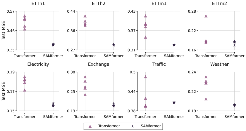
(a)

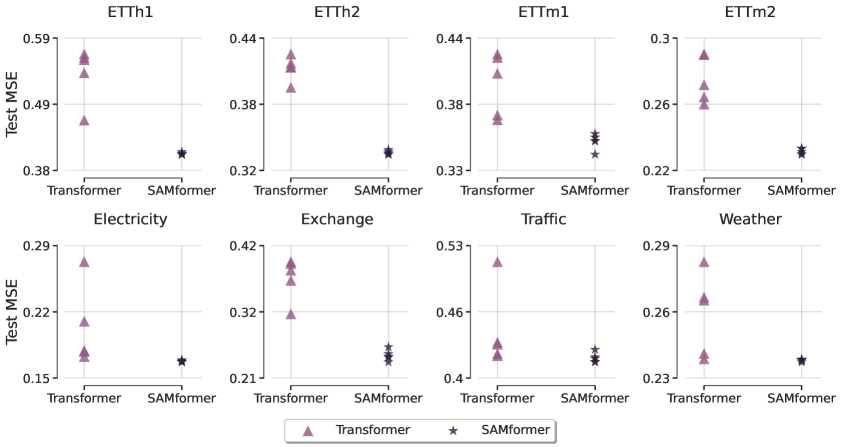
(b)

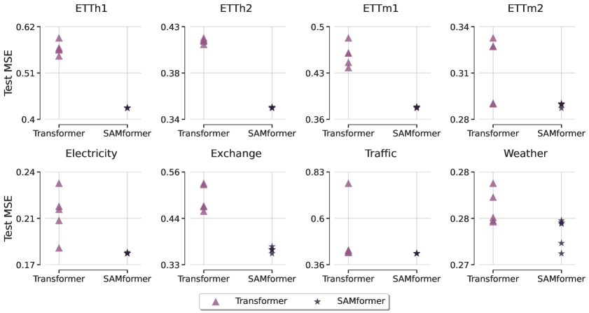
(a)

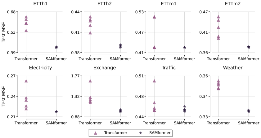
(b)

Figure 10: Test Mean Squared error on all datasets for a prediction horizon $H\in\{96,192,336,720\}$ across five different seed values for Transformer and SAMformer. This plot reveals a significant variance for the Transformer, as opposed to the minimal variance of SAMformer, showing the high impact of weight initialization on Transformer and the high resilience of SAMformer.

B.5 Faithful Signal Propagation

In this section, we consider Transformer, SAMformer, $\sigma$Reparam, which corresponds to Transformer with the rescaling proposed by Zhai et al., (2023) and SAMformer + $\sigma$Reparam which is SAMformer with the rescaling proposed by Zhai et al., (2023). For illustration, we plot a batch of attention matrices after training with prediction horizon $H=96$ (our primary study does not identify significant changes with the value of horizon) on Weather in Figure 12. While Transformer tends to ignore the importance of a feature on itself by having low values on the diagonal, we can see in the bottom left of Figure 12 that SAMformer strongly encourages these feature-to-feature correlations. A very distinctive pattern is observable, a near-identity attention reminiscent of He et al., (2023) and Trockman and Kolter, (2023). The former showcased that pre-trained vision models present similar patterns and both identified the benefits of such attention matrices for the propagation of information along the layers of deep transformers in NLP and computer vision. While in our setting, we have a single-layer transformer, this figure indicates that at the end of the training, self-information from features to themselves is not lost. In contrast, we see that $\sigma$Reparam leads to almost rank-$1$ matrices with identical columns. This confirms the theoretical insights from Theorem 2.3 that showed how rescaling the trainable weights with $\sigma$Reparam to limit the magnitude of $\lVert\mathbf{W}_{Q}\mathbf{W}_{K}^{\top}\rVert_{2}$ could hamper the rank of $\mathbf{X}\mathbf{W}_{Q}\mathbf{W}_{K}^{\top}\mathbf{X}^{\top}$ and of the attention matrix. Finally, we observe that naively combining SAMformer with $\sigma$Reparam does not solve the issues caused by the latter: while some diagonal patterns remain, most of the information has been lost. Moreover, combining both $\sigma$Reparam and SAMformer heavily increases the training time, as shown in Figure 11.

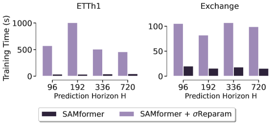
Figure 11: Using $\sigma$Reparam on top of SAMformer heavily increases the training time.

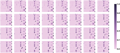
(a)

(b)

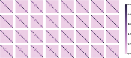
(c)

(d)

Figure 12: Batch of $32$ attention matrices on Weather with horizon $H=96$ after training different models. (a) Transformer. (b) $\sigma$Reparam (c) SAMformer. (d) SAMformer + $\sigma$Reparam.

Appendix C Ablation Study and Sensitivity Analysis

C.1 Sensitivity to the Prediction Horizon $H$.

In Figure 13, we show that SAMformer outperforms its best competitor, TSMixer trained with SAM, on $7$ out of $8$ datasets for all values of prediction horizon $H$. This demonstrates the robustness of SAMformer.

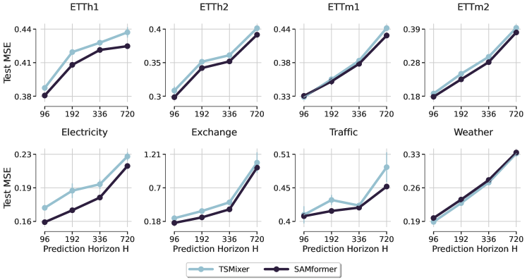
Figure 13: Evolution of the test MSE on all datasets for a prediction horizon $H\in\{96,192,336,720\}$. We display the average test MSE with a $95\%$ confidence interval. We see that SAMformer consistently performs well with a low variance. Despite its lightweight (Table 7), SAMformer surpasses TSMixer (trained with SAM) on $7$ out of $8$ datasets as shown in Table 1 and Table 6.

C.2 Sensitivity to the Neighborhood Size $\rho$.

In Figure 14, we display the evolution of test MSE of SAMformer and TSMixer with the values of neighborhood size $\rho$ for SAM. Overall, SAMformer has a smooth behavior with $\rho$, with a decreasing MSE and less variance. On the contrary, TSMixer is less stable and fluctuates more. On most of the datasets, the range of neighborhood seizes $\rho$ such that SAMformer is below TSMixer is large. The first value $\rho=0$ amounts to the usual minimization with Adam, which confirms that SAM always improves the performance of SAMformer. In addition, and despite its lightweight (Table 7), SAMformer achieves the lowest MSE on $7$ out of $8$ datasets, as shown in Table 1 and Table 6. It should be noted that compared to similar studies in computer vision (Chen et al.,, 2022), values of $\rho$ must be higher to effectively improve the generalization and flatten the loss landscapes. This follows from the high sharpness $\lambda_{max}$ observed in time series forecasting (Figure 5(a)) compared to computer vision models (Chen et al.,, 2022).

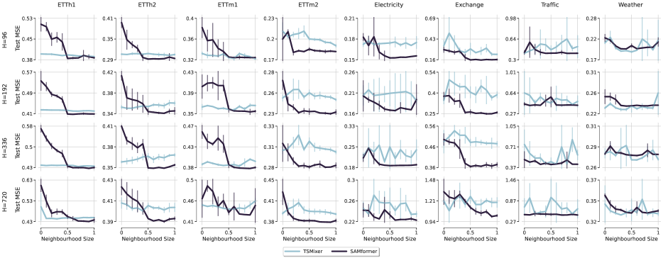
Figure 14: Evolution of the test MSE with the neighborhood size $\rho$ of SAM (Remark D.1). We display the average test MSE with a $95\%$ confidence interval. Overall, SAMformer has a smooth behavior with $\rho$, with a decreasing MSE and less variance. On the contrary, TSMixer is less stable and fluctuates more. On most of the datasets, the range of neighborhood seizes $\rho$ such that SAMformer is below TSMixer is large. The first value $\rho=0$ amounts to the usual minimization with Adam, which confirms that SAM always improves the performance of SAMformer. In addition, and despite its lightweight (Table 7), SAMformer achieves the lowest MSE on $7$ out of $8$ datasets, as shown in Table 1 and Table 6. It should be noted that compared to similar studies in computer vision (Chen et al.,, 2022), values of $\rho$ must be higher to effectively improve the generalization and flatten the loss landscapes.

C.3 Sensitivity to the Change of the Optimizer.

In our work, we considered the Adam optimizer (Kingma and Ba,, 2015) as it is the de-facto optimizer for transformer-based models (Ahn et al.,, 2023; Pan and Li,, 2022; Zhou et al.,, 2022, 2021; Chen et al.,, 2022). The superiority of Adam to optimize networks with attention has been empirically and theoretically studied, where recent works show that the SGD (Nesterov,, 1983) was not suitable for attention-based models (Ahn et al.,, 2023; Liu et al.,, 2020; Pan and Li,, 2022; Zhang et al.,, 2020). To ensure the thoroughness of our investigation, we conducted experiments on the synthetic dataset introduced in Eq. (2) and reported the results in Figure 15(a). As expected, we see that using SGD leads to high-magnitude losses and divergence. We also conducted the same experiments with the AdamW (Loshchilov and Hutter,, 2019) that incorporates the weight decay scheme in the adaptive optimizer Adam (Kingma and Ba,, 2015). We display the results obtained with weight decay factors $\mathrm{wd}=1\mathrm{e}{-3}$ in Figure 15(a) and with $\mathrm{wd}\in\{1\mathrm{e}{-5},1\mathrm{e}{-4}\}$ in Figure 15(b). When $\mathrm{wd}=1\mathrm{e}{-3}$, we observe that it does not converge. However, with $\mathrm{wd}\in\{1\mathrm{e}{-5},1\mathrm{e}{-4}\}$, we observe a similar behavior for Transformer than when it is trained with Adam (Figure 2). Hence, using AdamW does not lead to the significant benefits brought by SAM (Figure 1. As the optimization is very sensitive to the value of weight decay $\mathrm{wd}$, it motivates us to conduct our experiments with Adam.

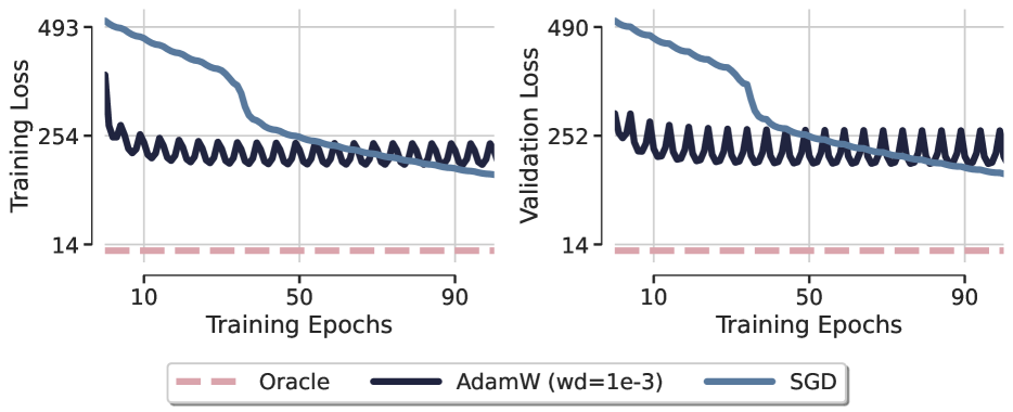
(a) SGD and AdamW with $\mathrm{wd}=1\mathrm{e}{-3}$

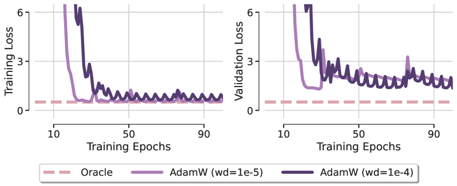
(b) AdamW with $\mathrm{wd}\in\{1\mathrm{e}{-5},1\mathrm{e}{-4}\}$.

Figure 15: Illustration of different optimizers on synthetic data generated with Eq. (2) where Oracle is the least-square solution. We saw in Figure 1 that with Adam, Transformer overfits and has poor performance while SAMformer smoothly reaches the oracle. (a) We can see that using SGD and Adam with weight decay $\mathrm{wd}=1\mathrm{e}{-5}$ leads to huge loss magnitudes and fails to converge. (b) With well-chosen weight decays ($\mathrm{wd}\in\{1\mathrm{e}{-3},1\mathrm{e}{-4}\}$), training Transformer with AdamW leads to similar performance than Adam. The overfitting is noticeable and the training is unstable. AdamW does not bring more stabilization and is very sensitive to the hyperparameters. Hence, this toy example motivates us to conduct our thorough experiments with the optimizer Adam.

C.4 Ablation on the Implementation.

This ablation study contrasts two variants of our model to showcase the effectiveness of Sharpness-Aware Minimization (SAM) and our attention approach. Identity Attention represents SAMformer with an attention weight matrix constrained to identity, illustrating that SAM does not simply reduce the attention weight matrix to identity, as performance surpasses this configuration. Temporal Attention is compared to our Transformer without SAM, highlighting our focus on treating feature correlations in the attention mechanism rather than temporal correlations.

Table 8: The Temporal Attention model is benchmarked against our Transformer model, which employs feature-based attention rather than time-step-based attention. We report in the last column the Overall improvement in MSE and MAE of Transformer over the Temporal Attention. This comparison reveals that channel-wise attention, i.e., focusing on features pairwise correlations, significantly boosts the performance, with a $12.97\%$ improvement in MSE and $18.09\%$ in MAE across all considered datasets.

Model	Metrics	H	ETTh1	ETTh2	ETTm1	ETTm2	Electricity	Exchange	Traffic	Weather	Overall Improvement
Temporal Attention	MSE	96	$0.496_{\pm 0.009}$	$0.401_{\pm 0.011}$	$0.542_{\pm 0.063}$	$0.330_{\pm 0.034}$	$0.291_{\pm 0.025}$	$0.684_{\pm 0.218}$	$0.933_{\pm 0.188}$	$0.225_{\pm 0.005}$	12.97%
		192	$0.510_{\pm 0.014}$	$0.414_{\pm 0.020}$	$0.615_{\pm 0.056}$	$0.394_{\pm 0.033}$	$0.294_{\pm 0.024}$	$0.434_{\pm 0.063}$	$0.647_{\pm 0.131}$	$0.254_{\pm 0.001}$
		336	$0.549_{\pm 0.017}$	$0.396_{\pm 0.014}$	$0.620_{\pm 0.046}$	$0.436_{\pm 0.081}$	$0.290_{\pm 0.016}$	$0.473_{\pm 0.014}$	$0.656_{\pm 0.113}$	$0.292_{\pm 0.000}$
		720	$0.604_{\pm 0.017}$	$0.396_{\pm 0.010}$	$0.694_{\pm 0.055}$	$0.469_{\pm 0.005}$	$0.307_{\pm 0.014}$	$1.097_{\pm 0.084}$	-	$0.346_{\pm 0.000}$
	MAE	96	$0.488_{\pm 0.007}$	$0.434_{\pm 0.006}$	$0.525_{\pm 0.040}$	$0.393_{\pm 0.020}$	$0.386_{\pm 0.014}$	$0.589_{\pm 0.096}$	$0.598_{\pm 0.072}$	$0.277_{\pm 0.004}$	18.09%
		192	$0.492_{\pm 0.010}$	$0.443_{\pm 0.015}$	$0.566_{\pm 0.032}$	$0.421_{\pm 0.019}$	$0.385_{\pm 0.014}$	$0.498_{\pm 0.033}$	$0.467_{\pm 0.072}$	$0.294_{\pm 0.001}$
		336	$0.517_{\pm 0.012}$	$0.440_{\pm 0.012}$	$0.550_{\pm 0.024}$	$0.443_{\pm 0.039}$	$0.383_{\pm 0.009}$	$0.517_{\pm 0.008}$	$0.469_{\pm 0.070}$	$0.320_{\pm 0.000}$
		720	$0.556_{\pm 0.009}$	$0.442_{\pm 0.006}$	$0.584_{\pm 0.027}$	$0.459_{\pm 0.004}$	$0.396_{\pm 0.012}$	$0.782_{\pm 0.041}$	-	$0.356_{\pm 0.000}$

Table 9: Identity Attention represents our SAMformer with the attention weight matrix constrained to an identity matrix. We report in the last column the Overall improvement in MSE and MAE of SAMformer over the Identity Attention. This setup demonstrates that naively fixing the attention matrix to the identity does not enable to match the performance of SAM, despite the near-identity attention matrices SAM showcases (see Appendix B.5 for more details). In particular, we observe an overall improvement of $11.93\%$ in MSE and $4.18\%$ in MAE across all the datasets.

Model	Metrics	H	ETTh1	ETTh2	ETTm1	ETTm2	Electricity	Exchange	Traffic	Weather	Overall Improvement
Identity Attention	MSE	96	$0.477_{\pm 0.059}$	$0.346_{\pm 0.055}$	$0.345_{\pm 0.027}$	$0.201_{\pm 0.035}$	$0.175_{\pm 0.015}$	$0.179_{\pm 0.031}$	$0.416_{\pm 0.037}$	$0.206_{\pm 0.019}$	11.93%
		192	$0.467_{\pm 0.074}$	$0.374_{\pm 0.031}$	$0.384_{\pm 0.042}$	$0.248_{\pm 0.016}$	$0.189_{\pm 0.022}$	$0.320_{\pm 0.070}$	$0.437_{\pm 0.041}$	$0.236_{\pm 0.002}$
		336	$0.512_{\pm 0.070}$	$0.372_{\pm 0.024}$	$0.408_{\pm 0.032}$	$0.303_{\pm 0.022}$	$0.211_{\pm 0.019}$	$0.443_{\pm 0.071}$	$0.500_{\pm 0.155}$	$0.277_{\pm 0.003}$
		720	$0.505_{\pm 0.107}$	$0.405_{\pm 0.012}$	$0.466_{\pm 0.043}$	$0.397_{\pm 0.029}$	$0.233_{\pm 0.019}$	$1.123_{\pm 0.076}$	$0.468_{\pm 0.021}$	$0.338_{\pm 0.009}$
	MAE	96	$0.473_{\pm 0.041}$	$0.395_{\pm 0.033}$	$0.376_{\pm 0.019}$	$0.294_{\pm 0.027}$	$0.283_{\pm 0.023}$	$0.320_{\pm 0.023}$	$0.301_{\pm 0.039}$	$0.259_{\pm 0.021}$	4.18%
		192	$0.463_{\pm 0.055}$	$0.413_{\pm 0.022}$	$0.399_{\pm 0.030}$	$0.321_{\pm 0.012}$	$0.291_{\pm 0.029}$	$0.418_{\pm 0.043}$	$0.314_{\pm 0.042}$	$0.278_{\pm 0.002}$
		336	$0.490_{\pm 0.049}$	$0.413_{\pm 0.015}$	$0.411_{\pm 0.019}$	$0.354_{\pm 0.018}$	$0.309_{\pm 0.021}$	$0.498_{\pm 0.041}$	$0.350_{\pm 0.106}$	$0.305_{\pm 0.003}$
		720	$0.496_{\pm 0.066}$	$0.438_{\pm 0.008}$	$0.444_{\pm 0.030}$	$0.406_{\pm 0.017}$	$0.322_{\pm 0.021}$	$0.788_{\pm 0.021}$	$0.325_{\pm 0.023}$	$0.347_{\pm 0.009}$

Appendix D Additional Background

D.1 Reversible Instance Normalization: RevIN

Overview.

Kim et al., 2021b recently proposed RevIN, a reversible instance normalization to reduce the discrepancy between the distributions of training and test data. Indeed, statistical properties of real-world time series, e.g. mean and variance, can change over time, leading to non-stationary sequences. This causes a distribution shift between training and test sets for the forecasting task. The RevIN normalization scheme is now widespread in deep learning approaches for time series forecasting (Chen et al.,, 2023; Nie et al.,, 2023). The RevIN normalization involves trainable parameters $(\bm{\beta},\bm{\gamma})\in\mathbb{R}^{K}\times\mathbb{R}^{K}$ and consists of two parts: a normalization step and a symmetric denormalization step. Before presenting them, we introduce for a given input time series $\mathbf{X}^{(i)}\in\mathcal{X}$ the empirical mean $\hat{\mu}[\mathbf{X}^{(i)}_{k}]$ and empirical standard deviation $\hat{\sigma}^{2}[\mathbf{X}^{(i)}_{k}]$ of its $k$-th feature $\mathbf{X}^{(i)}_{k}\in\mathbb{R}^{1\times L}$ as follows:

$$\begin{cases}&\hat{\mu}\left[\mathbf{X}^{(i)}_{k}\right]=\frac{1}{L}\sum_{t=1}^{L}\mathbf{X}^{(i)}_{kj}\\ &\hat{\sigma}^{2}\left[\mathbf{X}^{(i)}_{k}\right]=\frac{1}{L}\sum_{t=1}^{L}(\mathbf{X}^{(i)}_{kj}-\hat{\mu}[\mathbf{X}^{(i)}_{k}])^{2}\,.\end{cases}$$ (6)

The first one acts on the input sequence $\mathbf{X}^{(i)}$ and outputs the corresponding normalized sequence $\mathbf{\tilde{X}}^{(i)}\in\mathbb{R}^{K\times L}$ such that for all $k,t$,

$$\mathbf{\tilde{X}}^{(i)}_{kt}=\bm{\gamma}_{k}\left(\frac{\mathbf{X}^{(i)}_{kt}-\hat{\mu}\left[\mathbf{X}^{(i)}_{k}\right]}{\sqrt{\hat{\sigma}^{2}\left[\mathbf{X}^{(i)}_{k}\right]+\varepsilon}}\right)+\bm{\beta}_{k},$$ (7)

where $\varepsilon>0$ is a small constant to avoid dividing by $0$. The neural network’s input is then $\mathbf{\tilde{X}}^{(i)}$, instead of $\mathbf{X}^{(i)}$. The second step is applied to the output of the neural network $\mathbf{\tilde{Y}}^{(i)}$, such that the final output considered for the forecasting is the denormalized sequence $\mathbf{\hat{Y}}^{(i)}\in\mathbb{R}^{K\times H}$ such that for all $k,t$,

$$\mathbf{\hat{Y}}^{(i)}_{kt}=\sqrt{\hat{\sigma}^{2}\left[\mathbf{X}^{(i)}_{k}\right]+\varepsilon}\cdot\left(\frac{\mathbf{\tilde{Y}}^{(i)}_{kt}-\bm{\beta}_{k}}{\bm{\gamma}_{k}}\right)+\hat{\mu}\left[\mathbf{X}^{(i)}_{k}\right].$$ (8)

As stated in Kim et al., 2021b , $\hat{\mu},\hat{\sigma}^{2},\bm{\beta}$ and $\bm{\gamma}$ contain the non-stationary information of the input sequences $\mathbf{X}^{(i)}$.

End-to-end closed form with linear model and RevIN.

We consider a simple linear neural network. Formally, for any input sequence $\mathbf{X}\in\mathbb{R}^{D\times L}$, the prediction of $f_{\mathrm{lin}}\colon\mathbb{R}^{D\times L}\to\mathbb{R}^{D\times H}$ simply writes

$$f_{\mathrm{lin}}(\mathbf{X})=\mathbf{X}\mathbf{W}.$$ (9)

When combined with RevIN, the neural network $f_{\mathrm{lin}}$ is not directly applied to the input sequence but after the first normalization step of RevIN (Eq. (7)). An interesting benefit of the simplicity of $f_{\mathrm{lin}}$ is that it enables us to write its prediction in closed form, even when with RevIN. The proof is deferred to Appendix E.4. [Closed-form formulation] For any input sequence $\mathbf{X}\in\mathbb{R}^{K\times L}$, the output of the linear model $\mathbf{\hat{Y}}=f_{\mathrm{lin}}(\mathbf{X})\in\mathbb{R}^{K\times H}$ has entries

$$\mathbf{\hat{Y}}_{kt}=\hat{\mu}\left[\mathbf{X}_{k}\right]+\sum_{j=1}^{L}\left(\mathbf{X}_{kj}-\hat{\mu}\left[\mathbf{X}_{k}\right]\right)\mathbf{W}_{jt}-\frac{\bm{\beta}_{k}}{\bm{\gamma}_{k}}\sqrt{\hat{\sigma}^{2}\left[\mathbf{X}_{k}\right]+\varepsilon}\left(1-\sum_{j=1}^{L}\mathbf{W}_{jt}\right),$$ (10)

Proposition 9 highlights the fact that the $k$-th variable of the outputs $\mathbf{\hat{Y}}$ only depends on $k$-th variable of the input sequence $\mathbf{X}$. It leads to channel-independent forecasting, although we did not explicitly enforce it. (10) can be seen as a linear interpolation around the mean $\hat{\mu}$ with a regularization term on the network parameters $\mathbf{W}$ involving the non-stationary information $\hat{\sigma}^{2},\bm{\beta},\bm{\gamma}$. Moreover, the output sequence $\mathbf{\hat{Y}}$ can be written in a more compact and convenient matrix formulation as follows

$$\mathbf{\hat{Y}}=\mathbf{X}\mathbf{W}+\bm{\xi}^{(\mathbf{X},\mathbf{W},\bm{\beta},\bm{\gamma})},$$ (11)

where $\bm{\xi}^{(\mathbf{X},\mathbf{W},\bm{\beta},\bm{\gamma})}\in\mathbb{R}^{K\times H}$ with entry $\left(\hat{\mu}\left[\mathbf{X}_{k}\right]-\frac{\bm{\beta}_{k}}{\bm{\gamma}_{k}}\sqrt{\hat{\sigma}^{2}\left[\mathbf{X}_{k}\right]+\varepsilon}\right)\left(1-\sum_{j=1}^{L}\mathbf{W}_{jt}\right)$ in the $k$-th row and $t$-th column. The proof is deferred to Appendix E.5. With this formulation, the predicted sequence can be seen as a sum of a linear term $\mathbf{X}\mathbf{W}$ and a residual term $\bm{\xi}^{(\mathbf{X},\mathbf{W},\bm{\beta},\bm{\gamma})}$ that takes into account the first and second moments of each variable $\mathbf{X}_{k}$, which is reminiscent of the linear regression model.

D.2 Sharpness-aware minimization (SAM)

Regularizing with the sharpness.

Standard approaches consider a parametric family of models $f_{\bm{\omega}}$ and aim to find parameters $\bm{\omega}$ that minimize a training objective $\mathcal{L}_{\mathrm{train}}\left(\bm{\omega}\right)$, used as a tractable proxy to the true generalization error $\mathcal{L}_{\mathrm{test}}\left(\bm{\omega}\right)$. Most deep learning pipelines rely on first-order optimizers, e.g. SGD (Nesterov,, 1983) or Adam (Kingma and Ba,, 2015), that disregard higher-order information such as the curvature, despite its connection to generalization (Dziugaite and Roy,, 2017; Chaudhari et al.,, 2017; Keskar et al.,, 2017). As $\mathcal{L}_{\mathrm{train}}$ is usually non-convex in $\bm{\omega}$, with multiple local or global minima, solving $\min_{\bm{\omega}}\mathcal{L}_{\mathrm{train}}\left(\bm{\omega}\right)$ may still lead to high generalization error $\mathcal{L}_{\mathrm{test}}\left(\bm{\omega}\right)$. To alleviate this issue, Foret et al., (2021) propose to regularize the training objective with the sharpness, defined as follows [Sharpness, Foret et al., (2021)] For a given $\rho\geq 0$, the sharpness of $\mathcal{L}_{\mathrm{train}}$ at $\bm{\omega}$ writes

$$s\left(\bm{\omega},\rho\right)\coloneqq\max_{\lVert\bm{\epsilon}\rVert_{2}\leq\rho}\mathcal{L}_{\mathrm{train}}\left(\bm{\omega}+\bm{\epsilon}\right)-\mathcal{L}_{\mathrm{train}}\left(\bm{\omega}\right).$$ (12)

Remark D.1 (Interpretation of $\rho$).

Instead of simply minimizing the training objective $\mathcal{L}_{\mathrm{train}}$, SAM searches for parameters $\bm{\omega}$ achieving both low training loss and low curvature in a ball $\mathcal{B}(\bm{\omega},\rho)$. The hyperparameter $\rho\geq 0$ corresponds to the size of the neighborhood on which the parameters search is done. In particular, taking $\rho=0$ is equivalent to the usual minimization of $\mathcal{L}_{\mathrm{train}}$.

In particular, SAM incorporates sharpness in the learning objective, resulting in the problem of minimizing w.r.t $\bm{\omega}$

$$\mathcal{L}_{\mathrm{train}}^{\textrm{SAM}}(\bm{\omega})\coloneqq\underbrace{\max_{\lVert\bm{\epsilon}\rVert_{2}\leq\rho}\mathcal{L}_{\mathrm{train}}\left(\bm{\omega}+\bm{\epsilon}\right)}_{=\mathcal{L}_{\mathrm{train}}\left(\bm{\omega}\right)+s\left(\bm{\omega},\rho\right)}\,.$$ (13)

Gradient updates.

As the exact solution to the inner maximization in Eq. (13) is hard to compute, the authors of (Foret et al.,, 2021) approximate it with the following first-order Taylor expansion

$$\bm{\epsilon}^{*}\left(\bm{\omega}\right) \coloneqq\operatorname*{arg\,max}_{\lVert\bm{\epsilon}\rVert_{2}\leq\rho}\mathcal{L}_{\mathrm{train}}\left(\bm{\omega}+\bm{\epsilon}\right)$$

$$\approx\operatorname*{arg\,max}_{\lVert\bm{\epsilon}\rVert_{2}\leq\rho}\mathcal{L}_{\mathrm{train}}\left(\bm{\omega}\right)+\bm{\epsilon}^{\top}\nabla\mathcal{L}_{\mathrm{train}}\left(\bm{\omega}\right)$$

$$=\operatorname*{arg\,max}_{\lVert\bm{\epsilon}\rVert_{2}\leq\rho}\bm{\epsilon}^{\top}\nabla\mathcal{L}_{\mathrm{train}}\left(\bm{\omega}\right)\,,$$ (14)

where the solution of (D.2) writes $\bm{\hat{\epsilon}}\left(\bm{\omega}\right)=\rho\frac{\nabla\mathcal{L}_{\mathrm{train}}\left(\bm{\omega}\right)}{\lVert\nabla\mathcal{L}_{\mathrm{train}}\left(\bm{\omega}\right)\rVert_{2}}$. It leads to the following gradient update

$$\bm{\omega}_{t+1}=\bm{\omega}_{t}-\eta\nabla\mathcal{L}_{\mathrm{train}}\left(\bm{\omega}_{t}+\rho\frac{\nabla\mathcal{L}_{\mathrm{train}}\left(\bm{\omega}\right)}{\lVert\nabla\mathcal{L}_{\mathrm{train}}\left(\bm{\omega}\right)\rVert_{2}}\right)\,,$$

where $\eta$ is the learning rate.

Appendix E Proofs

E.1 Notations

To ease the readability of the proofs, we recall the following notations. We denote scalar values by regular letters (e.g., parameter $\lambda$), vectors by bold lowercase letters (e.g., vector $\mathbf{x}$), and matrices by bold capital letters (e.g., matrix $\mathbf{M}$). For a matrix $\mathbf{M}\in\mathbb{R}^{n\times m}$, we denote by $\mathbf{M}_{i}$ its $i$-th row, by $\mathbf{M}_{\cdot,j}$ its $j$-th column, by $m_{ij}$ its entries and by $\mathbf{M}^{\top}$ its transpose. We denote the trace of a matrix $\mathbf{M}$ by $\operatorname{Tr}\left(\mathbf{M}\right)$, its rank by $\operatorname{rank}\left(\mathbf{M}\right)$ and its Frobenius norm by $\lVert\mathbf{M}\rVert_{\mathrm{F}}$. We denote $\bm{\sigma}\left(\mathbf{M}\right)\coloneqq\left(\sigma_{1}(\mathbf{M}),\dots,\sigma_{\tilde{n}}(\mathbf{M})\right)$ the vector of singular values of $\mathbf{M}$ in non-decreasing order, with $\tilde{n}=\min\{n,m\}$ and the specific notation $\sigma_{\mathrm{min}}(\mathbf{M}),\sigma_{\mathrm{max}}(\mathbf{M})$ for the minimum and maximum singular values, respectively. We denote by $\lVert\mathbf{M}\rVert_{*}=\sum_{i=1}^{\tilde{n}}\sigma_{i}(\mathbf{M})$ its nuclear norm and by $\lVert\mathbf{M}\rVert_{2}=\sigma_{\mathrm{max}}(\mathbf{M})$ its spectral norm. When $\mathbf{M}$ is square with $n=m$, we denote $\bm{\lambda}\left(\mathbf{M}\right)\coloneqq\left(\lambda_{1}(\mathbf{M}),\dots,\lambda_{n}(\mathbf{M})\right)$ the vector of singular values of $\mathbf{M}$ in non-decreasing order and the specific notation $\lambda_{\mathrm{min}}(\mathbf{M}),\lambda_{\mathrm{max}}(\mathbf{M})$ for the minimum and maximum singular values, respectively. For a vector $\mathbf{x}$, its transpose writes $\mathbf{x}^{\top}$ and its usual Euclidean norm writes $\lVert\mathbf{x}\rVert$. The identity matrix of size $n\times n$ is denoted by $\mathbf{I}_{n}$. The vector of size $n$ with each entry equal to $1$ is denoted by $\mathbbm{1}_{n}$. The notation $\mathbf{M}\succcurlyeq\mathbf{0}$ indicates that $\mathbf{M}$ is positive semi-definite.

E.2 Proof of Proposition 2.2

We first recall the following technical lemmas. Let $\mathbf{S}\in\mathbb{R}^{n\times m}$ and $\mathbf{B}\in\mathbb{R}^{m\times m}$. If $\mathbf{B}$ has full rank, then

$$\operatorname{rank}\left(\mathbf{S}\mathbf{B}\right)=\operatorname{rank}\left(\mathbf{B}\mathbf{S}\right)=\operatorname{rank}\left(\mathbf{S}\right).$$

Proof.

Let $\mathbf{F}_{1}\coloneq\{\mathbf{S}\mathbf{u}|\mathbf{u}\in\mathbb{R}^{m}\}\subset\mathbb{R}^{n}$ and $\mathbf{F}_{2}\coloneq\{\left(\mathbf{S}\mathbf{B}\right)\mathbf{u}|\mathbf{u}\in\mathbb{R}^{m}\}\subset\mathbb{R}^{n}$ be the vector spaces generated by the columns of $\mathbf{S}$ and $\mathbf{S}\mathbf{B}$ respectively. By definition, the rank of a matrix is the dimension of the vector space generated by its columns (equivalently by its rows). We will show that $\mathbf{F}_{1}$ and $\mathbf{F}_{2}$ coincides. Let $\mathbf{v}\in\mathbf{F}_{1}$, i.e., there exists $\mathbf{u}\in\mathbb{R}^{m}$ such that $\mathbf{v}=\mathbf{S}\mathbf{u}$. As $\mathbf{B}$ is full rank, the operator $\mathbf{x}\to\mathbf{B}\mathbf{x}$ is bijective. It follows that there always exists some $\mathbf{z}\in\mathbb{R}^{m}$ such that $\mathbf{u}=\mathbf{B}\mathbf{z}$. Then, we have

$$\mathbf{v}=\mathbf{S}\mathbf{u}=\mathbf{S}\left(\mathbf{B}\mathbf{z}\right)=\left(\mathbf{S}\mathbf{B}\right)\mathbf{z},$$

which means that $\mathbf{v}\in\mathbf{F}_{2}$. As $\mathbf{v}$ was taken arbitrarily in $\mathbf{F}_{1}$, we have proved that $\mathbf{F}_{1}\subset\mathbf{F}_{2}$. Conversely, consider $\mathbf{y}\in\mathbf{F}_{2}$, i.e., we can write $\mathbf{y}=\left(\mathbf{S}\mathbf{B}\right)\mathbf{z}$ for some $\mathbf{z}\in\mathbb{R}^{m}$. It can then be seen that

$$\mathbf{y}=\left(\mathbf{S}\mathbf{B}\right)\mathbf{z}=\mathbf{S}\left(\mathbf{B}\mathbf{z}\right),$$

which means that $\mathbf{y}\in\mathbf{F}_{1}$. Again, as $\mathbf{y}$ was taken arbitrarily, we have proved that $\mathbf{F}_{1}\subset\mathbf{F}_{2}$. In the end, we demonstrated that $\mathbf{F}_{1}$ and $\mathbf{F}_{2}$ coincide, hence they have the same dimension. By definition of the rank, $\mathbf{S}$ and $\mathbf{S}\mathbf{B}$ have the same rank. Similar arguments can be used to show that $\mathbf{S}$ and $\mathbf{B}\mathbf{S}$ have the same rank, which concludes the proof. ∎

The next lemma is a well-known result in matrix analysis and can be found in Horn and Johnson, (1991, Theorem 4.4.5). For the sake of self-consistency, we recall it below along with a sketch of the original proof. (see Horn and Johnson,, 1991, Theorem 4.4.5, p. 281). Let $\mathbf{S}\in\mathbb{R}^{n\times m},\mathbf{B}=\mathbb{R}^{p\times q}$ and $\mathbf{C}\in\mathbb{R}^{n\times q}$. There exist matrices $\mathbf{Y}\in\mathbb{R}^{m\times q}$ and $\mathbf{Z}\in\mathbb{R}^{n\times p}$ such that $\mathbf{S}\mathbf{Y}-\mathbf{Z}\mathbf{B}=\mathbf{C}$ if, and only if,

$$\operatorname{rank}\left(\begin{bmatrix}\mathbf{S}&\mathbf{C}\\ \mathbf{0}&\mathbf{B}\end{bmatrix}\right)=\operatorname{rank}\left(\begin{bmatrix}\mathbf{S}&\mathbf{0}\\ \mathbf{0}&\mathbf{B}\end{bmatrix}\right).$$

Proof.

Assume that there exists $\mathbf{Y}\in\mathbb{R}^{m\times q}$ and $\mathbf{Z}\in\mathbb{R}^{n\times p}$ such that $\mathbf{S}\mathbf{Y}-\mathbf{Z}\mathbf{B}=\mathbf{C}$. We recall that the following equality holds

$$\begin{bmatrix}\mathbf{S}&\mathbf{S}\mathbf{Y}-\mathbf{Z}\mathbf{B}\\ \mathbf{0}&\mathbf{B}\end{bmatrix}=\begin{bmatrix}\mathbf{I}_{m}&-\mathbf{Y}\\ \mathbf{0}&\mathbf{I}_{q}\end{bmatrix}\begin{bmatrix}\mathbf{S}&\mathbf{0}\\ \mathbf{0}&\mathbf{B}\end{bmatrix}\begin{bmatrix}\mathbf{I}_{n}&\mathbf{Z}\\ \mathbf{0}&\mathbf{I}_{p}\end{bmatrix}.$$ (15)

Using Lemma E.2 twice on the right-hand-side of Eq. (15), we obtain

$$\operatorname{rank}\left(\begin{bmatrix}\mathbf{S}&\mathbf{S}\mathbf{Y}-\mathbf{Z}\mathbf{B}\\ \mathbf{0}&\mathbf{B}\end{bmatrix}\right)=\operatorname{rank}\left(\begin{bmatrix}\mathbf{S}&\mathbf{0}\\ \mathbf{0}&\mathbf{B}\end{bmatrix}\right).$$

Using $\mathbf{S}\mathbf{Y}-\mathbf{Z}\mathbf{B}=\mathbf{C}$ concludes the proof for the direct sense of the equivalence.
Conversely, assume that

$$\operatorname{rank}\left(\begin{bmatrix}\mathbf{S}&\mathbf{C}\\ \mathbf{0}&\mathbf{B}\end{bmatrix}\right)=\operatorname{rank}\left(\begin{bmatrix}\mathbf{S}&\mathbf{0}\\ \mathbf{0}&\mathbf{B}\end{bmatrix}\right).$$

Since two matrices have the same rank if, and only if, they are equivalent, we know that there exists $\mathbf{Q}\in\mathbb{R}^{(n+p)\times(n+p)},\mathbf{U}\in\mathbb{R}^{(m+q)\times(m+q)}$ non-singular such that

$$\begin{bmatrix}\mathbf{S}&\mathbf{C}\\ \mathbf{0}&\mathbf{B}\end{bmatrix}=\mathbf{Q}\begin{bmatrix}\mathbf{S}&\mathbf{0}\\ \mathbf{0}&\mathbf{B}\end{bmatrix}\mathbf{U}.$$ (16)

The rest of the proof in Horn and Johnson, (1991) is constructive and relies on Eq. (16) to exhibit $\mathbf{Y}\in\mathbb{R}^{m\times q}$ and $\mathbf{Z}\in\mathbb{R}^{n\times p}$ such that $\mathbf{S}\mathbf{Y}-\mathbf{Z}\mathbf{B}=\mathbf{C}$. This concludes the proof of the equivalence. ∎

We now proceed to the proof of Proposition 2.2.

Proof.

Applying Lemma E.2 with $\mathbf{S}=\mathbf{P}$, $\mathbf{B}=\mathbf{0}$, $\mathbf{C}=\mathbf{X}\mathbf{W}_{\mathrm{toy}}$ and $\mathbf{W}$ in the role of $\mathbf{Y}$ ensures that there exists $\mathbf{W}\in\mathbb{R}^{L\times H}$ such that $\mathbf{P}\mathbf{W}=\mathbf{X}\mathbf{W}_{\mathrm{toy}}$ if and only if $\operatorname{rank}\left(\left[\mathbf{P}\quad\mathbf{X}\mathbf{W}_{\mathrm{toy}}\right]\right)=\operatorname{rank}\left(\mathbf{P}\right)$, which concludes the proof. ∎

E.3 Proof of Proposition 2.3

We first prove the following technical lemmas. While these lemmas are commonly used and, for most of them, straightforward to prove, they are very useful to demonstrate Proposition 2.3. [Trace of a product of matrix] Let $\mathbf{S},\mathbf{B}\in\mathbb{R}^{n\times n}$ be symmetric matrices with $\mathbf{B}$ positive semi-definite. We have

$$\lambda_{\mathrm{min}}\left(\mathbf{S}\right)\operatorname{Tr}\left(\mathbf{B}\right)\leq\operatorname{Tr}\left(\mathbf{S}\mathbf{B}\right)\leq\lambda_{\mathrm{max}}\left(\mathbf{S}\right)\operatorname{Tr}\left(\mathbf{B}\right).$$

Proof.

The spectral theorem ensures the existence of $\mathbf{P}\in\mathbb{R}^{n\times n}$ orthogonal, i.e., $\mathbf{P}^{\top}\mathbf{P}=\mathbf{P}\mathbf{P}^{\top}=\mathbf{I}_{n}$, and $\bm{\Lambda}\in\mathbb{R}^{n\times n}$ diagonal with the eigenvalues of $\mathbf{S}$ as entries such that $\mathbf{S}=\mathbf{P}\bm{\Lambda}\mathbf{P}^{\top}$. Benefiting from the properties of the trace operator, we have

$$\operatorname{Tr}\left(\mathbf{S}\mathbf{B}\right) =\operatorname{Tr}\left(\mathbf{I}_{n}\mathbf{S}\mathbf{B}\right)$$

$$=\operatorname{Tr}\left(\underbrace{\mathbf{P}\mathbf{P}^{\top}}_{=\mathbf{I}_{n}}\mathbf{S}\mathbf{B}\right) \mathbf{P}$$ (orthogonality of )

$$=\operatorname{Tr}\left(\mathbf{P}^{\top}\mathbf{S}\mathbf{B}\mathbf{P}\right)$$ (cyclic property of trace)

$$=\operatorname{Tr}\left(\mathbf{P}^{\top}\mathbf{P}\bm{\Lambda}\mathbf{P}^{\top}\mathbf{B}\mathbf{P}\right)$$ (Spectral theorem)

$$=\operatorname{Tr}\left(\underbrace{\mathbf{P}^{\top}\mathbf{P}}_{=\mathbf{I}_{n}}\bm{\Lambda}\mathbf{P}^{\top}\mathbf{B}\mathbf{P}\right) \mathbf{P}$$ (orthogonality of )

$$=\operatorname{Tr}\left(\bm{\Lambda}\mathbf{P}^{\top}\mathbf{B}\mathbf{P}\right).$$

We introduce $\tilde{\mathbf{B}}=\mathbf{P}^{\top}\mathbf{B}\mathbf{P}=[\tilde{b}_{ij}]_{ij}$. It follows from the definition of $\bm{\Lambda}$ that

$$\operatorname{Tr}\left(\mathbf{S}\mathbf{B}\right)=\operatorname{Tr}\left(\bm{\Lambda}\mathbf{P}^{\top}\mathbf{B}\mathbf{P}\right)=\operatorname{Tr}\left(\bm{\Lambda}\tilde{\mathbf{B}}\right)=\sum_{i}\lambda_{i}\left(\mathbf{S}\right)\tilde{b}_{ii}.$$ (17)

We would like to write the $\tilde{b}_{ij}$ with respect to the $p_{ij},b_{ij}$ the elements of $\mathbf{P},\mathbf{B}$, respectively. As $\mathbf{P}$ is orthogonal, we know that its columns $(\mathbf{e}_{i})_{i=0}^{n}$ form an orthonormal basis of $\mathbb{R}^{n}$. Hence, the entry $(i,j)$ of $\bm{\Lambda}\mathbf{P}^{\top}\mathbf{B}\mathbf{P}$, writes as follows:

$$\tilde{b}_{ij} =\sum_{kl}p_{ki}b_{ij}p_{jk}$$

$$=\sum_{k}p_{ki}\underbrace{\left(\sum_{l}b_{ij}p_{jk}\right)}_{\left[\mathbf{B}\mathbf{e}_{j}\right]_{k}}$$

$$=\sum_{k}p_{ki}\left[\mathbf{B}\mathbf{e}_{j}\right]_{k}$$

$$=e_{i}^{\top}\mathbf{B}\mathbf{e}_{j}\geq 0. \mathbf{B}\succcurlyeq\mathbf{0}$$ ()

Hence, as $\mathbf{B}$ is positive semi-definite, the $\tilde{b}_{ij}$ are nonnegative. It follows that

$$\lambda_{\mathrm{min}}\left(\mathbf{S}\right)\sum_{i}\tilde{b}_{ii}\leq\sum_{i}\lambda_{i}\left(\mathbf{S}\right)\underbrace{\tilde{b}_{ii}}_{\geq 0}\leq\lambda_{\mathrm{max}}\left(\mathbf{S}\right)\sum_{i}\tilde{b}_{ii}.$$ (18)

Moreover, using the definition of $\tilde{\mathbf{B}}$, the orthogonality of $\mathbf{P}$ and the cyclic property of the trace operation, we have

$$\sum_{i}\tilde{b}_{ii}=\operatorname{Tr}\left(\tilde{\mathbf{B}}\right)=\operatorname{Tr}\left(\mathbf{P}^{\top}\mathbf{B}\mathbf{P}\right)=\operatorname{Tr}\left(\underbrace{\mathbf{P}\mathbf{P}^{\top}}_{=\mathbf{I}_{n}}\mathbf{B}\right)=\operatorname{Tr}\left(\mathbf{B}\right).$$

Combining this last equality with Eq. (17) and Eq. (18) concludes the proof, i.e.,

$$\lambda_{\mathrm{min}}\left(\mathbf{S}\right)\operatorname{Tr}\left(\mathbf{B}\right)\leq\operatorname{Tr}\left(\mathbf{S}\mathbf{B}\right)\leq\lambda_{\mathrm{max}}\left(\mathbf{S}\right)\operatorname{Tr}\left(\mathbf{B}\right).$$ (19)

∎

[Power of symmetric matrices] Let $\mathbf{S}\in\mathbb{R}^{n\times n}$ be symmetric. The spectral theorem ensures the existence of $\mathbf{P}\in\mathbb{R}^{n\times n}$ orthogonal, i.e., $\mathbf{P}^{\top}\mathbf{P}=\mathbf{P}\mathbf{P}^{\top}=\mathbf{I}_{n}$, and $\bm{\Lambda}\in\mathbb{R}^{n\times n}$ diagonal with the eigenvalues of $\mathbf{S}$ as entries such that $\mathbf{S}=\mathbf{P}\bm{\Lambda}\mathbf{P}^{\top}$. For any integer $n\geq 1$, we have

$$\mathbf{S}^{n}=\mathbf{P}\bm{\Lambda}^{n}\mathbf{P}^{\top}.$$

In particular, the eigenvalues of $\mathbf{S}^{n}$ are equal to the eigenvalues of $\mathbf{S}$ to the power of $n$.

Proof.

Let $n\geq 1$ be an integer. We have

$$\mathbf{S}^{n} =\left(\mathbf{P}\bm{\Lambda}\mathbf{P}^{\top}\right)^{n}$$

$$=\underbrace{\mathbf{P}\bm{\Lambda}\mathbf{P}^{\top}\times\mathbf{P}\bm{\Lambda}\mathbf{P}^{\top}\times\dots\times\mathbf{P}\bm{\Lambda}\mathbf{P}^{\top}\times\mathbf{P}\bm{\Lambda}\mathbf{P}^{\top}}_{\times n}$$

$$=\underbrace{\mathbf{P}\bm{\Lambda}\times\bm{\Lambda}\mathbf{P}^{\top}\dots\mathbf{P}\bm{\Lambda}\times\bm{\Lambda}\mathbf{P}^{\top}}_{\times n} \mathbf{P}$$ (orthogonality of )

$$=\mathbf{P}\underbrace{\bm{\Lambda}\times\bm{\Lambda}\times\dots\times\bm{\Lambda}\times\bm{\Lambda}}_{\times n}\mathbf{P}^{\top} \mathbf{P}$$ (orthogonality of )

$$=\mathbf{P}\bm{\Lambda}^{n}\mathbf{P}^{\top}.$$

The diagonality of $\bm{\Lambda}$ suffices to deduct the remark on the eigenvalues of $\mathbf{S}^{n}$. ∎

[Case of equality between eigenvalues and singular values] Let $\mathbf{S}\in\mathbb{R}^{n\times n}$ be symmetric and positive semi-definite. Then the $i$-th eigenvalue and the $i$-th singular value of $\mathbf{S}$ are equal, i.e., for all $i\in\llbracket 1,n\rrbracket$, we have

$$\lambda_{i}\left(\mathbf{S}\right)=\sigma_{i}\left(\mathbf{S}\right).$$

Proof.

Let $i\in\llbracket 1,n\rrbracket$. By definition of singular value, we have

$$\sigma_{i}\left(\mathbf{S}\right) \coloneqq\sqrt{\lambda_{i}\left(\mathbf{S}^{\top}\mathbf{S}\right)}$$

$$=\sqrt{\lambda_{i}\left(\mathbf{S}^{2}\right)} \mathbf{S}$$ ( is symmetric)

$$=\sqrt{\lambda_{i}\left(\mathbf{S}\right)^{2}}$$ (Lemma E.3)

$$=\lvert\lambda_{i}\left(\mathbf{S}\right)\rvert$$

$$=\lambda_{i}\left(\mathbf{S}\right). \mathbf{S}\succcurlyeq\mathbf{0}$$ ()

∎

Let $\mathbf{X}\in\mathbb{R}^{D\times L}$ be an input sequence and $\mathbf{S}\in\mathbb{R}^{L\times L}$ be a positive semi-definite matrix. Then, $\mathbf{X}\mathbf{S}\mathbf{X}^{\top}$ is positive semi-definite.

Proof.

It is clear that $\mathbf{X}\mathbf{S}\mathbf{X}^{\top}\in\mathbb{R}^{L\times L}$ is symmetric. Let $\mathbf{u}\in\mathbb{R}^{L}$. We have:

$$\mathbf{u}^{\top}\mathbf{X}\mathbf{S}\mathbf{X}^{\top}\mathbf{u} =\left(\mathbf{X}^{\top}\mathbf{u}\right)^{\top}\mathbf{S}\left(\mathbf{X}^{\top}\mathbf{u}\right)\geq 0. \mathbf{S}\succcurlyeq\mathbf{0}$$ ()

As $\mathbf{u}$ was arbitrarily chosen, we have proved that $\mathbf{X}\mathbf{S}\mathbf{X}^{\top}$ is positive semi-definite. ∎

We now proceed to the proof of Theorem 2.3.

Proof.

We recall that $\mathbf{W}_{Q}\mathbf{W}_{K}^{\top}$ is symmetric and positive semi-definite, we have

$$\lVert\mathbf{X}\mathbf{W}_{Q}\mathbf{W}_{K}^{\top}\mathbf{X}^{\top}\rVert_{*} =\operatorname{Tr}\left(\sqrt{\left(\mathbf{X}\mathbf{W}_{Q}\mathbf{W}_{K}^{\top}\mathbf{X}^{\top}\right)^{\top}\mathbf{X}\mathbf{W}_{Q}\mathbf{W}_{K}^{\top}\mathbf{X}^{\top}}\right)$$

$$=\operatorname{Tr}\left(\sqrt{\mathbf{X}\mathbf{W}_{K}\mathbf{W}_{Q}^{\top}\mathbf{X}^{\top}\mathbf{X}\mathbf{W}_{Q}\mathbf{W}_{K}^{\top}\mathbf{X}^{\top}}\right)$$

$$=\operatorname{Tr}\left(\sqrt{\mathbf{X}\mathbf{W}_{Q}\mathbf{W}_{K}^{\top}\mathbf{X}^{\top}\mathbf{X}\mathbf{W}_{Q}\mathbf{W}_{K}^{\top}\mathbf{X}^{\top}}\right)$$ (symmetry)

$$=\operatorname{Tr}\left(\sqrt{\left(\mathbf{X}\mathbf{W}_{Q}\mathbf{W}_{K}^{\top}\mathbf{X}^{\top}\right)^{2}}\right)$$

$$=\operatorname{Tr}\left(\mathbf{X}\mathbf{W}_{Q}\mathbf{W}_{K}^{\top}\mathbf{X}^{\top}\right) \mathbf{S}=\mathbf{W}_{Q}\mathbf{W}_{K}^{\top}$$ (Lemma E.3 with )

$$=\operatorname{Tr}\left(\mathbf{X}^{\top}\mathbf{X}\mathbf{W}_{Q}\mathbf{W}_{K}^{\top}\right).$$ (cyclic property of the trace)

Using the fact that $\mathbf{X}^{\top}\mathbf{X}$ is positive semi-definite (Lemma E.3 with $\mathbf{S}=\mathbf{I}_{L}$), and that $\mathbf{W}_{Q}\mathbf{W}_{K}^{\top}$ is symmetric, Lemma E.3 can be applied with $\mathbf{M}=\mathbf{W}_{Q}\mathbf{W}_{K}^{\top}$ and $\mathbf{B}=\mathbf{X}^{\top}\mathbf{X}$. It leads to:

$$\lVert\mathbf{X}\mathbf{W}_{Q}\mathbf{W}_{K}^{\top}\mathbf{X}^{\top}\rVert_{*}=\operatorname{Tr}\left(\mathbf{X}^{\top}\mathbf{X}\mathbf{W}_{Q}\mathbf{W}_{K}^{\top}\right) \leq\lambda_{\mathrm{max}}\left(\mathbf{W}_{Q}\mathbf{W}_{K}^{\top}\right)\operatorname{Tr}\left(\mathbf{X}^{\top}\mathbf{X}\right)\,.$$ (Lemma E.3)

As $\mathbf{W}_{Q}\mathbf{W}_{K}^{\top}$ is positive semi-definite, Lemma E.3 ensure

$$\lambda_{\mathrm{max}}\left(\mathbf{W}_{Q}\mathbf{W}_{K}^{\top}\right)=\sigma_{\mathrm{max}}\left(\mathbf{W}_{Q}\mathbf{W}_{K}^{\top}\right)=\lVert\mathbf{W}_{Q}\mathbf{W}_{K}^{\top}\rVert_{2}$$

by definition of the spectral norm $\lVert\cdot\rVert_{2}$. Recalling that by definition, $\operatorname{Tr}\left(\mathbf{X}^{\top}\mathbf{X}\right)=\lVert\mathbf{X}\rVert_{\mathrm{F}}^{2}$ concludes the proof, i.e.,

$$\lVert\mathbf{X}\mathbf{W}_{Q}\mathbf{W}_{K}^{\top}\mathbf{X}^{\top}\rVert_{*}\leq\lVert\mathbf{W}_{Q}\mathbf{W}_{K}^{\top}\rVert_{2}\lVert\mathbf{X}\rVert_{\mathrm{F}}^{2}.$$

∎

E.4 Proof of Proposition 9

Proof.

Let $k\in\llbracket 1,K\rrbracket$ and $t\in\llbracket 1,H\rrbracket$. We have

$$\mathbf{\hat{Y}}_{kt} =\sqrt{\hat{\sigma}^{2}\left[\mathbf{X}_{k}\right]+\varepsilon}\cdot\left(\frac{\mathbf{\tilde{y}}_{kt}-\bm{\beta}_{k}}{\bm{\gamma}_{k}}\right)+\hat{\mu}\left[\mathbf{X}_{k}\right],$$ (from (8))

$$=\sqrt{\hat{\sigma}^{2}\left[\mathbf{x}_{k}\right]+\varepsilon}\cdot\left(\frac{\sum_{j=1}^{L}\mathbf{\tilde{X}}_{kj}\mathbf{W}_{jt}-\bm{\beta}_{k}}{\bm{\gamma}_{k}}\right)+\hat{\mu}\left[\mathbf{X}_{k}\right],$$ (from (9))

$$=\frac{\sqrt{\hat{\sigma}^{2}\left[\mathbf{X}_{k}\right]+\varepsilon}}{\bm{\gamma}_{k}}\cdot\sum_{j=1}^{L}\mathbf{\tilde{X}}_{kj}\mathbf{W}_{jt}-\frac{\bm{\beta}_{k}}{\bm{\gamma}_{k}}\sqrt{\hat{\sigma}^{2}\left[\mathbf{X}_{k}\right]+\varepsilon}+\hat{\mu}\left[\mathbf{X}_{k}\right]$$

$$=\frac{\sqrt{\hat{\sigma}^{2}\left[\mathbf{X}_{k}\right]+\varepsilon}}{\bm{\gamma}_{k}}\cdot\sum_{j=1}^{L}\left(\bm{\gamma}_{k}\left(\frac{\mathbf{X}_{kj}-\hat{\mu}\left[\mathbf{x}_{k}\right]}{\sqrt{\hat{\sigma}^{2}\left[\mathbf{X}_{k}\right]+\varepsilon}}\right)+\bm{\beta}_{k}\right)\mathbf{W}_{jt}-\frac{\bm{\beta}_{k}}{\bm{\gamma}_{k}}\sqrt{\hat{\sigma}^{2}\left[\mathbf{x}_{k}\right]+\varepsilon}+\hat{\mu}\left[\mathbf{X}_{k}\right],$$ (from (7))

$$=\sum_{j=1}^{L}\left(\mathbf{X}_{kj}-\hat{\mu}\left[\mathbf{X}_{k}\right]\right)\mathbf{W}_{jt}+\frac{\bm{\beta}_{k}}{\bm{\gamma}_{k}}\sqrt{\hat{\sigma}^{2}\left[\mathbf{X}_{k}\right]+\varepsilon}\left(\sum_{j=1}^{L}\mathbf{W}_{jt}-1\right)+\hat{\mu}\left[\mathbf{X}_{k}\right]$$

$$=\hat{\mu}\left[\mathbf{X}_{k}\right]+\sum_{j=1}^{L}\left(\mathbf{X}_{kj}-\hat{\mu}\left[\mathbf{X}_{k}\right]\right)\mathbf{W}_{jt}-\frac{\bm{\beta}_{k}}{\bm{\gamma}_{k}}\sqrt{\hat{\sigma}^{2}\left[\mathbf{X}_{k}\right]+\varepsilon}\left(1-\sum_{j=1}^{L}\mathbf{W}_{jt}\right).$$

∎

E.5 Matrix formulation of $\mathbf{\hat{Y}}$ in Eq. (11)

Let $k\in\llbracket 1,K\rrbracket$ and $t\in\llbracket 1,H\rrbracket$. From Proposition 9, we have

$$\mathbf{\hat{Y}}_{kt} =\hat{\mu}\left[\mathbf{X}_{k}\right]+\sum_{j=1}^{L}\left(\mathbf{X}_{kj}-\hat{\mu}\left[\mathbf{X}_{k}\right]\right)\mathbf{W}_{jt}-\frac{\bm{\beta}_{k}}{\bm{\gamma}_{k}}\sqrt{\hat{\sigma}^{2}\left[\mathbf{X}_{k}\right]+\varepsilon}\left(1-\sum_{j=1}^{L}\mathbf{W}_{jt}\right)$$

$$=\sum_{j=1}^{L}\mathbf{X}_{kj}\mathbf{W}_{jt}+\left(\hat{\mu}\left[\mathbf{X}_{k}\right]-\frac{\bm{\beta}_{k}}{\bm{\gamma}_{k}}\sqrt{\hat{\sigma}^{2}\left[\mathbf{X}_{k}\right]+\varepsilon}\right)\cdot\left(1-\sum_{j=1}^{L}\mathbf{W}_{jt}\right).$$

Gathering in matrix formulation concludes the proof.

References

- Ahn et al., (2023) Ahn, K., Cheng, X., Song, M., Yun, C., Jadbabaie, A., and Sra, S. (2023). Linear attention is (maybe) all you need (to understand transformer optimization).
- Anagnostidis et al., (2022) Anagnostidis, S., Biggio, L., Noci, L., Orvieto, A., Singh, S. P., and Lucchi, A. (2022). Signal propagation in transformers: Theoretical perspectives and the role of rank collapse. In Oh, A. H., Agarwal, A., Belgrave, D., and Cho, K., editors, Advances in Neural Information Processing Systems.
- Box and Jenkins, (1990) Box, G. E. P. and Jenkins, G. (1990). Time Series Analysis, Forecasting and Control. Holden-Day, Inc., USA.
- Box et al., (1974) Box, G. E. P., Jenkins, G. M., and MacGregor, J. F. (1974). Some Recent Advances in Forecasting and Control. Journal of the Royal Statistical Society Series C, 23(2):158–179.
- (5) California Department of Transportation (n.d.). Traffic dataset.
- Candès and Recht, (2012) Candès, E. and Recht, B. (2012). Exact matrix completion via convex optimization. Commun. ACM, 55(6):111–119.
- Caron et al., (2021) Caron, M., Touvron, H., Misra, I., Jégou, H., Mairal, J., Bojanowski, P., and Joulin, A. (2021). Emerging properties in self-supervised vision transformers. In Proceedings of the International Conference on Computer Vision (ICCV).
- Casolaro et al., (2023) Casolaro, A., Capone, V., Iannuzzo, G., and Camastra, F. (2023). Deep learning for time series forecasting: Advances and open problems. Information, 14(11).
- Čepulionis and Lukoševičiūtė, (2016) Čepulionis, P. and Lukoševičiūtė, K. (2016). Electrocardiogram time series forecasting and optimization using ant colony optimization algorithm. Mathematical Models in Engineering, 2(1):69–77.
- Chaudhari et al., (2017) Chaudhari, P., Choromanska, A., Soatto, S., LeCun, Y., Baldassi, C., Borgs, C., Chayes, J., Sagun, L., and Zecchina, R. (2017). Entropy-SGD: Biasing gradient descent into wide valleys. In International Conference on Learning Representations.
- Chen and Tao, (2021) Chen, R. and Tao, M. (2021). Data-driven prediction of general hamiltonian dynamics via learning exactly-symplectic maps. In Meila, M. and Zhang, T., editors, Proceedings of the 38th International Conference on Machine Learning, volume 139 of Proceedings of Machine Learning Research, pages 1717–1727. PMLR.
- Chen et al., (2023) Chen, S.-A., Li, C.-L., Arik, S. O., Yoder, N. C., and Pfister, T. (2023). TSMixer: An all-MLP architecture for time series forecasting. Transactions on Machine Learning Research.
- Chen et al., (2022) Chen, X., Hsieh, C.-J., and Gong, B. (2022). When vision transformers outperform resnets without pre-training or strong data augmentations. In International Conference on Learning Representations.
- Cirstea et al., (2022) Cirstea, R.-G., Guo, C., Yang, B., Kieu, T., Dong, X., and Pan, S. (2022). Triformer: Triangular, variable-specific attentions for long sequence multivariate time series forecasting. In Raedt, L. D., editor, Proceedings of the Thirty-First International Joint Conference on Artificial Intelligence, IJCAI-22, pages 1994–2001. International Joint Conferences on Artificial Intelligence Organization. Main Track.
- Daneshmand et al., (2020) Daneshmand, H., Kohler, J., Bach, F., Hofmann, T., and Lucchi, A. (2020). Batch normalization provably avoids rank collapse for randomly initialised deep networks. In Proceedings of the 34th International Conference on Neural Information Processing Systems, NIPS’20, Red Hook, NY, USA. Curran Associates Inc.
- Devlin et al., (2018) Devlin, J., Chang, M.-W., Lee, K., and Toutanova, K. (2018). Bert: Pre-training of deep bidirectional transformers for language understanding.
- Dong et al., (2021) Dong, Y., Cordonnier, J.-B., and Loukas, A. (2021). Attention is not all you need: pure attention loses rank doubly exponentially with depth. In Meila, M. and Zhang, T., editors, Proceedings of the 38th International Conference on Machine Learning, volume 139 of Proceedings of Machine Learning Research, pages 2793–2803. PMLR.
- Dosovitskiy et al., (2021) Dosovitskiy, A., Beyer, L., Kolesnikov, A., Weissenborn, D., Zhai, X., Unterthiner, T., Dehghani, M., Minderer, M., Heigold, G., Gelly, S., Uszkoreit, J., and Houlsby, N. (2021). An image is worth 16x16 words: Transformers for image recognition at scale. In International Conference on Learning Representations.
- Dziugaite and Roy, (2017) Dziugaite, G. K. and Roy, D. M. (2017). Computing nonvacuous generalization bounds for deep (stochastic) neural networks with many more parameters than training data. In Proceedings of the 33rd Annual Conference on Uncertainty in Artificial Intelligence (UAI).
- Fan et al., (2019) Fan, C., Zhang, Y., Pan, Y., Li, X., Zhang, C., Yuan, R., Wu, D., Wang, W., Pei, J., and Huang, H. (2019). Multi-horizon time series forecasting with temporal attention learning. In Proceedings of the 25th ACM SIGKDD International Conference on Knowledge Discovery & Data Mining, KDD ’19, page 2527–2535, New York, NY, USA. Association for Computing Machinery.
- Foret et al., (2021) Foret, P., Kleiner, A., Mobahi, H., and Neyshabur, B. (2021). Sharpness-aware minimization for efficiently improving generalization. In International Conference on Learning Representations.
- Glorot and Bengio, (2010) Glorot, X. and Bengio, Y. (2010). Understanding the difficulty of training deep feedforward neural networks. In Teh, Y. W. and Titterington, M., editors, Proceedings of the Thirteenth International Conference on Artificial Intelligence and Statistics, volume 9 of Proceedings of Machine Learning Research, pages 249–256, Chia Laguna Resort, Sardinia, Italy. PMLR.
- He et al., (2023) He, B., Martens, J., Zhang, G., Botev, A., Brock, A., Smith, S. L., and Teh, Y. W. (2023). Deep transformers without shortcuts: Modifying self-attention for faithful signal propagation. In The Eleventh International Conference on Learning Representations.
- Horn and Johnson, (1991) Horn, R. A. and Johnson, C. R. (1991). Topics in Matrix Analysis. Cambridge University Press.
- Keskar et al., (2017) Keskar, N. S., Mudigere, D., Nocedal, J., Smelyanskiy, M., and Tang, P. T. P. (2017). On large-batch training for deep learning: Generalization gap and sharp minima. In International Conference on Learning Representations.
- (26) Kim, H., Papamakarios, G., and Mnih, A. (2021a). The lipschitz constant of self-attention. In Meila, M. and Zhang, T., editors, Proceedings of the 38th International Conference on Machine Learning, volume 139 of Proceedings of Machine Learning Research, pages 5562–5571. PMLR.
- (27) Kim, T., Kim, J., Tae, Y., Park, C., Choi, J.-H., and Choo, J. (2021b). Reversible instance normalization for accurate time-series forecasting against distribution shift. In International Conference on Learning Representations.
- Kingma and Ba, (2015) Kingma, D. and Ba, J. (2015). Adam: A method for stochastic optimization. In International Conference on Learning Representations (ICLR), San Diega, CA, USA.
- Kitaev et al., (2020) Kitaev, N., Kaiser, L., and Levskaya, A. (2020). Reformer: The efficient transformer. In International Conference on Learning Representations.
- (30) Lai, G., Chang, W.-C., Yang, Y., and Liu, H. (2018a). Modeling long- and short-term temporal patterns with deep neural networks. In The 41st International ACM SIGIR Conference on Research & Development in Information Retrieval, SIGIR ’18, page 95–104, New York, NY, USA. Association for Computing Machinery.
- (31) Lai, G., Chang, W.-C., Yang, Y., and Liu, H. (2018b). Modeling long- and short-term temporal patterns with deep neural networks. In Association for Computing Machinery, SIGIR ’18, page 95–104, New York, NY, USA.
- Li et al., (2019) Li, S., Jin, X., Xuan, Y., Zhou, X., Chen, W., Wang, Y.-X., and Yan, X. (2019). Enhancing the locality and breaking the memory bottleneck of transformer on time series forecasting. In Wallach, H., Larochelle, H., Beygelzimer, A., d'Alché-Buc, F., Fox, E., and Garnett, R., editors, Advances in Neural Information Processing Systems, volume 32. Curran Associates, Inc.
- Liu et al., (2020) Liu, L., Liu, X., Gao, J., Chen, W., and Han, J. (2020). Understanding the difficulty of training transformers. In Proceedings of the 2020 Conference on Empirical Methods in Natural Language Processing (EMNLP 2020).
- Liu et al., (2022) Liu, S., Yu, H., Liao, C., Li, J., Lin, W., Liu, A. X., and Dustdar, S. (2022). Pyraformer: Low-complexity pyramidal attention for long-range time series modeling and forecasting. In International Conference on Learning Representations.
- Loshchilov and Hutter, (2017) Loshchilov, I. and Hutter, F. (2017). SGDR: Stochastic gradient descent with warm restarts. In International Conference on Learning Representations.
- Loshchilov and Hutter, (2019) Loshchilov, I. and Hutter, F. (2019). Decoupled weight decay regularization. In International Conference on Learning Representations.
- (37) Max Planck Institute (n.d.). Weather dataset.
- Nesterov, (1983) Nesterov, Y. (1983). A method for solving the convex programming problem with convergence rate . Proceedings of the USSR Academy of Sciences, 269:543–547.
- Nie et al., (2023) Nie, Y., Nguyen, N. H., Sinthong, P., and Kalagnanam, J. (2023). A time series is worth 64 words: Long-term forecasting with transformers. In The Eleventh International Conference on Learning Representations.
- OpenAI, (2023) OpenAI (2023). Gpt-4 technical report.
- Pan and Li, (2022) Pan, Y. and Li, Y. (2022). Toward understanding why adam converges faster than SGD for transformers. In OPT 2022: Optimization for Machine Learning (NeurIPS 2022 Workshop).
- Radford et al., (2018) Radford, A., Narasimhan, K., Salimans, T., and Sutskever, I. (2018). Improving language understanding by generative pre-training. 2018 OpenAI Tech Report.
- Rangapuram et al., (2018) Rangapuram, S. S., Seeger, M. W., Gasthaus, J., Stella, L., Wang, Y., and Januschowski, T. (2018). Deep state space models for time series forecasting. In Bengio, S., Wallach, H., Larochelle, H., Grauman, K., Cesa-Bianchi, N., and Garnett, R., editors, Advances in Neural Information Processing Systems, volume 31. Curran Associates, Inc.
- Recht, (2011) Recht, B. (2011). A simpler approach to matrix completion. J. Mach. Learn. Res., 12(null):3413–3430.
- Recht et al., (2010) Recht, B., Fazel, M., and Parrilo, P. A. (2010). Guaranteed minimum-rank solutions of linear matrix equations via nuclear norm minimization. SIAM Review, 52(3):471–501.
- Salinas et al., (2020) Salinas, D., Flunkert, V., Gasthaus, J., and Januschowski, T. (2020). Deepar: Probabilistic forecasting with autoregressive recurrent networks. International Journal of Forecasting, 36(3):1181–1191.
- Sen et al., (2019) Sen, R., Yu, H.-F., and Dhillon, I. (2019). Think globally, act locally: a deep neural network approach to high-dimensional time series forecasting. In Proceedings of the 33rd International Conference on Neural Information Processing Systems, Red Hook, NY, USA. Curran Associates Inc.
- Sonkavde et al., (2023) Sonkavde, G., Dharrao, D. S., Bongale, A. M., Deokate, S. T., Doreswamy, D., and Bhat, S. K. (2023). Forecasting stock market prices using machine learning and deep learning models: A systematic review, performance analysis and discussion of implications. International Journal of Financial Studies, 11(3).
- Sorjamaa et al., (2007) Sorjamaa, A., Hao, J., Reyhani, N., Ji, Y., and Lendasse, A. (2007). Methodology for long-term prediction of time series. Neurocomputing, 70(16):2861–2869. Neural Network Applications in Electrical Engineering Selected papers from the 3rd International Work-Conference on Artificial Neural Networks (IWANN 2005).
- Touvron et al., (2021) Touvron, H., Cord, M., Douze, M., Massa, F., Sablayrolles, A., and Jegou, H. (2021). Training data-efficient image transformers and distillation through attention. In Meila, M. and Zhang, T., editors, Proceedings of the 38th International Conference on Machine Learning, volume 139 of Proceedings of Machine Learning Research, pages 10347–10357. PMLR.
- Touvron et al., (2023) Touvron, H., Lavril, T., Izacard, G., Martinet, X., Lachaux, M.-A., Lacroix, T., Rozière, B., Goyal, N., Hambro, E., Azhar, F., Rodriguez, A., Joulin, A., Grave, E., and Lample, G. (2023). Llama: Open and efficient foundation language models. cite arxiv:2302.13971.
- Trockman and Kolter, (2023) Trockman, A. and Kolter, J. Z. (2023). Mimetic initialization of self-attention layers. In Proceedings of the 40th International Conference on Machine Learning, ICML’23. JMLR.org.
- (53) UCI (n.d.). Electricity dataset.
- Vaswani et al., (2017) Vaswani, A., Shazeer, N., Parmar, N., Uszkoreit, J., Jones, L., Gomez, A. N., Kaiser, L. u., and Polosukhin, I. (2017). Attention is all you need. In Guyon, I., Luxburg, U. V., Bengio, S., Wallach, H., Fergus, R., Vishwanathan, S., and Garnett, R., editors, Advances in Neural Information Processing Systems, volume 30. Curran Associates, Inc.
- Wu et al., (2021) Wu, H., Xu, J., Wang, J., and Long, M. (2021). Autoformer: Decomposition transformers with Auto-Correlation for long-term series forecasting. In Advances in Neural Information Processing Systems.
- Zamir et al., (2022) Zamir, S. W., Arora, A., Khan, S., Hayat, M., Khan, F. S., and Yang, M.-H. (2022). Restormer: Efficient transformer for high-resolution image restoration. In CVPR.
- Zeng et al., (2023) Zeng, A., Chen, M., Zhang, L., and Xu, Q. (2023). Are transformers effective for time series forecasting? In Proceedings of the AAAI Conference on Artificial Intelligence.
- Zhai et al., (2023) Zhai, S., Likhomanenko, T., Littwin, E., Busbridge, D., Ramapuram, J., Zhang, Y., Gu, J., and Susskind, J. M. (2023). Stabilizing transformer training by preventing attention entropy collapse. In Krause, A., Brunskill, E., Cho, K., Engelhardt, B., Sabato, S., and Scarlett, J., editors, Proceedings of the 40th International Conference on Machine Learning, volume 202 of Proceedings of Machine Learning Research, pages 40770–40803. PMLR.
- Zhang et al., (2022) Zhang, H., Wu, C., Zhang, Z., Zhu, Y., Lin, H., Zhang, Z., Sun, Y., He, T., Mueller, J., Manmatha, R., Li, M., and Smola, A. (2022). Resnest: Split-attention networks. In Proceedings of the IEEE/CVF Conference on Computer Vision and Pattern Recognition (CVPR) Workshops, pages 2736–2746.
- Zhang et al., (2020) Zhang, J., Karimireddy, S. P., Veit, A., Kim, S., Reddi, S., Kumar, S., and Sra, S. (2020). Why are adaptive methods good for attention models? In Larochelle, H., Ranzato, M., Hadsell, R., Balcan, M., and Lin, H., editors, Advances in Neural Information Processing Systems, volume 33, pages 15383–15393. Curran Associates, Inc.
- Zhou et al., (2021) Zhou, H., Zhang, S., Peng, J., Zhang, S., Li, J., Xiong, H., and Zhang, W. (2021). Informer: Beyond efficient transformer for long sequence time-series forecasting. In The Thirty-Fifth AAAI Conference on Artificial Intelligence, AAAI 2021, Virtual Conference, volume 35, pages 11106–11115. AAAI Press.
- Zhou et al., (2022) Zhou, T., Ma, Z., Wen, Q., Wang, X., Sun, L., and Jin, R. (2022). FEDformer: Frequency enhanced decomposed transformer for long-term series forecasting. In Proc. 39th International Conference on Machine Learning (ICML 2022).