Simple Tilings of Nilpotent Lie Groups

Abstract.

We define simple tilings in the general context of a $G$-tiling on a Riemannian homogeneous space $\mathcal{M}$ to be tilings by "almost linear" simplices. As evidence that this definition is natural, we prove that a natural class of tilings of $\mathcal{M}$ are MLD to simple ones. We demonstrate the utility of this definition by generalizing previously known results about simple tilings of $\mathbb{R}^{n}$. In particular, it is shown that a simple tiling space of a connected, simply connected, rational, nilpotent Lie group is homeomorphic to a rational tiling space, and therefore a fiber bundle over a nilmanifold. We further sketch a proof of the fact that there is an isomorphism between C̆ech cohomology and pattern equivariant cohomology of simple tilings in connected, simply connected, nilpotent Lie groups.

1. Introduction

Since the discovery of physical quasi-crystals in the mid twentieth century, there has been growing interest in properly defining and studying such structures in a mathematical framework. This has lead to defining mathematical quasi-crystals in Euclidean space both as certain Delaunay sets and as tilings, providing two different perspectives which are often equivalent in a strong sense. In [17] it is demonstrated that for sufficiently nice tilings of $\mathbb{R}^{n}$, one may construct a Delaunay set which in turn induces a tiling MLD to the original. The induced tiling has elegant geometric and combinatorial data, allowing one to simplify the study of many tilings to so-called simple tilings. Dually, keeping track of the intermediate Delaunay set allows one to more clearly utilize the underlying structure of $\mathbb{R}^{n}$ without worrying about the geometry of the tiles.

Many results about tilings in $\mathbb{R}^{n}$, therefore, take this simplicity assumption for granted. Unfortunately, the definition of simple tilings in $\mathbb{R}^{n}$ does not extend immediately to more general contexts; it is required that tiles are convex polytopes, which is not a reasonable assumption in spaces such as nilpotent Lie groups.

For this reason, we seek to generalize the definition a simple tiling to be one for which the tiles are "almost linear" simplices (defined precisely in Section 3). To demonstrate that this simplification is not too strong, we prove the following theorem which relates simple tilings to a natural class of tilings which we call "geometrically normal" (defined precisely in Section 2).

theoremsimpleTilings Let $\mathcal{M}$ be a Riemannian homogeneous space. Given a geometrically normal $G$-tiling $\mathcal{T}$ of $\mathcal{M}$, there is a simple tiling $\mathcal{T}_{\Delta}$ which is MLD to $\mathcal{T}$.

We expect that many theorems of simple tilings for $\mathbb{R}^{n}$ will extend to simple tilings of more general spaces with this new definition. To demonstrate this, and to further justify that our definition of simple tilings is indeed appropriate, we generalize two facts about tilings of $\mathbb{R}^{n}$ to the nilpotent setting.

In [19], it is shown that a large class of tiling spaces are inverse limits of branched manifolds. In this process it is shown that such tiling spaces look locally like the product of a Cantor set together with a certain group $G$. Motivated by the work of Anderson and Putnam on tiling dynamics, Sadun and Williams show in [21] that, for simple tilings of $\mathbb{R}^{n}$, these local pieces actually fit together to create a fiber bundle over the torus $\mathbb{T}^{n}$, providing some topological insight into these dynamical systems.

The question is posed at the end of [19] whether this fiber bundle construction extends to other spaces. Specifically, it is asked whether the Cantor set neighborhoods constructed can be "stitched together" to yield a fiber bundle over a compact manifold. The question is further refined by asking whether that compact manifold is the quotient of $G$ by a cocompact subgroup. As an application of Section 1, we apply the proof technique of Sadun and Williams to expand the class of tilings for which the answer to both questions is "yes".

theoremnilpotentFiberBundles Let $\mathscr{T}$ be a simple tiling space over a connected, simply connected, rational nilpotent Lie group $\mathbb{G}$. Then there is a cocompact lattice $\Lambda\subseteq\mathbb{G}$ such that $\mathscr{T}$ is a fiber bundle over the nilmanifold $\mathbb{G}/\Lambda$.

Since such Lie groups naturally generalize $\mathbb{R}^{n}$, it is fitting that the theory of mathematical quasi-crystals be generalized to this setting as well. Furthermore, the study of tilings in such groups is not without precedent: in recent years, there has been a growing interest in the study of mathematical quasi-crystals in connected, simply-connected, nilpotent Lie groups. Recent work in this direction can be found, for example, in [1] and [14]. Indeed, such work serves as motivation for the present paper.

We provide further evidence that our notion of simple tilings is appropriate by presenting and sketching the proof of the following theorem, generalizing another well-known fact from simple Euclidean tilings to the setting of nilpotent Lie groups.

theoremPECohomology Given a simple tiling $\mathcal{T}$ of $\mathbb{G}$, the (real or integer) pattern equivariant cohomology of $\mathcal{T}$ is isomorphic to the C̆ech cohomology of the hull $\Omega_{\mathcal{T}}$ of $\mathcal{T}$ (with real or integer coefficients, respectively).

In Section 2, we present the relevant tools for studying tiling spaces and review some of the well-known results for simple tilings of $\mathbb{R}^{n}$, as well as examples of tilings more generally. In Section 3, we discuss Delaunay sets in detail and state a few necessary results about Delaunay triangulations of manifolds. In Section 4, we generalize the definition of simple tilings of homogeneous Riemannian spaces, and apply the previous two sections to prove Section 1. In Section 5, we provide the necessary background for connected, simply connected, nilpotent Lie groups. In Section 6, we prove Section 1, demonstrating that our definition of "simple tilings" is a useful generalization. In Section 7, we provide another application in a sketch of the proof of Section 1. Finally, in Section 8, we conclude by presenting directions of ongoing and future work.

Acknowledgements

The author would like to thank his advisor, Fedya Manin, for inspiration and constant guidance throughout this project. The author would also like to thank Lorenzo Sadun for his kindness in correcting some of the author’s mistakes in the background material. All remaining confusion and error (fatal or otherwise) belong solely to the author.

2. Tiling Spaces

In this section, we present the required background on tiling spaces. The first few subsections are very general, and it is helpful to keep mind the particular case $G=\mathcal{M}$ a nilpotent Lie group acting on itself by left translation, with basepoint $m_{0}=e$ the origin. Observe that while we consider left-action, the theory can be made to work for right-actions as well without any substantial change. We will eventually narrow in to well-known results about simple Euclidean tilings. All tilings in this paper are assumed to have finite local complexity (see below) unless otherwise stated.

2.1. Basic Preliminaries

Let $(\mathcal{M},m_{0})$ be a complete, based Riemannian manifold with a distance function $d_{\mathcal{M}}$. A tiling of $\mathcal{M}$ is a subdivision of $\mathcal{M}$ into topological disks called tiles which intersect only along their boundaries. We will say that $\mathcal{T}$ is normal if tiles are uniformly bounded topological disks which intersect in connected set. We will further say that a tiling is geometrically normal if, in addition, the intersection of tiles are piecewise smooth submanifolds which are themselves closed topological disks. Unless otherwise stated, we assume that all tilings are geometrically normal.

Given a tiling $\mathcal{T}$ of $\mathcal{M}$ and a subset $U\subseteq\mathcal{M}$, the patch of $\mathcal{T}$ around $U$ is

$$[U]_{\mathcal{T}}=\left\{\text{tiles which intersect the closure $\overline{U}$ nontrivially}\right\}.$$

If the tiling $\mathcal{T}$ is clear from context, we drop the subscript and simply write $[U]=[U]_{\mathcal{T}}$.

Fix a closed subgroup $G\leq\mathrm{Isom}(\mathcal{M})$ acting transitively on $\mathcal{M}$. Suppose moreover that $d_{\mathcal{M}}$ is left-invariant under $G$, and that $G$ has a norm $\|\cdot\|$ associated to it. We will be interested in studying tilings which have nice properties relative to $G$. We therefore say that a tiling is a $G$-tiling of $\mathcal{M}$ when we want to track the action of $G$.

We may often switch between $\mathcal{T}$ and $\mathcal{M}$, using each to denote both the manifold as well as the tiling, though we try to use $\mathcal{T}$ whenever the tiles are relevant. We call a set $\mathcal{P}$ of tiles in $\mathcal{M}$ a set of prototiles for $\mathcal{T}$ if, for every tile $T$ in $\mathcal{T}$, there is a prototile $P\in\mathcal{P}$ and some $g\in G$ such that $g.P=T$, where $g.P:=\left\{g.p\;\middle|\;p\in P\right\}$. Given a tiling $\mathcal{T}$, we define $g.\mathcal{T}$ to be the tiling for which all tiles have been translated by $g$. That is, $g.\mathcal{T}=\left\{g.T\;\middle|\;T\in\mathcal{T}\right\}$.

The action of $G$ defines an equivalence relation on patches of $\mathcal{T}$. Indeed, given patches $[U],[V]\subseteq\mathcal{T}$, we say that $[U]\sim_{G}[V]$ if $[U]_{g.\mathcal{T}}=[V]_{\mathcal{T}}$ for some $g\in G$. If the group $G$ is clear from context, we will simply write $[U]\sim[V]$.

We say that $\mathcal{T}$ has finite local complexity (or simply FLC) if for any compact $K\subseteq\mathcal{M}$, the set of equivalence classes of translates of $K$ is finite. That is,

$$\#\left\{[gK]\;\middle|\;g\in G\right\}/\sim\;\;<\infty$$

for every compact set $K$. We will often consider compact sets of the form $K=B_{r}(m_{0})$ where $m_{0}\in\mathcal{M}$ is the basepoint. As $G$ is a transitive action, and $d_{\mathcal{M}}$ is left-invariant, $\mathcal{T}$ has FLC precisely when

$$\#\left\{[B_{r}(x)]\;\middle|\;x\in\mathcal{M}\right\}/\sim\;\;<\infty$$

for all $r>0$. Observe for example that if $\mathcal{T}$ has FLC, then $\#\mathcal{P}<\infty$. All tilings in this section and throughout the paper are assumed to have finite local complexity.

Here, we define a metric, called the tiling metric, on all $G$-tilings of $\mathcal{M}$. We want this metric to describe when one tiling looks like another at sufficiently large scales around the basepoint, up to a "small" transformation by $G$. If $\mathcal{T}$ and $\mathcal{T}^{\prime}$ are $G$ tilings of $\mathcal{M}$, we define

$$R(\mathcal{T},\mathcal{T}^{\prime}):=\inf\left\{r>0\;\middle|\;[B_{r}(m_{0})]_{g.\mathcal{T}}=[B_{r}(m_{0})]_{g^{\prime}.\mathcal{T}^{\prime}}\text{ for some $g,g^{\prime}\in G$ with $\|g\|,\|g^{\prime}\|<\frac{1}{2r}$}\right\}.$$

The tiling metric is then defined by

$$d_{G,\mathcal{M}}(\mathcal{T},\mathcal{T}^{\prime}):=\min\left\{1,\frac{1}{R(\mathcal{T},\mathcal{T}^{\prime})}\right\}.$$

A tiling space is a collection $\mathscr{T}$ of tilings which is complete with respect to the tiling metric, and invariant under the action of $G$, so that $g.\mathcal{T}\in\mathscr{T}$ for every $\mathcal{T}\in\mathscr{T}$. Given a tiling $\mathcal{T}$, the smallest tiling space containing $\mathcal{T}$ is called the hull of $\mathcal{T}$, and will be denoted by $\Omega_{G,\mathcal{T}}$, or simply $\Omega_{\mathcal{T}}$ if context allows. Equivalently, if $\mathcal{O}(\mathcal{T}):=\left\{g.\mathcal{T}\;\middle|\;g\in G\right\}$ is the orbit of $\mathcal{T}$ under the action of $G$, then $\Omega_{G,\mathcal{T}}=\overline{\mathcal{O}(\mathcal{T})}$. Though we are interested in tiling spaces in general here, it is often instructive to keep the hull of a particular tiling in mind as a primary example of such spaces.

2.2. Gähler Complexes and Inverse Limits

The following result from [19] applied very broadly, showing that a large class of tiling spaces can be also be constructed as the inverse limit of certain branched manifolds.

Note.

The theorem as stated in the original paper does not make any reference to the normality of the tilings. We add in the assumption that the tiling space is geometrically normal for reasons to be explained in Subsection 2.4

Theorem 2.1 ([19, §2]).

Let $\Omega$ be a geometrically normal, FLC $G$-tiling space over a based Riemannian homogeneous space $\mathcal{M}$. Then for each $n\in\mathbb{N}$ there is a branched manifold $\Gamma_{n}$ with $\dim\Gamma_{n}=\dim G$, and a continuous map $\sigma_{n}:\Gamma_{n}\to\Gamma_{n-1}$, such that $\Omega=\varprojlim(\Gamma_{n},\sigma_{n})$.

We do not reproduce the proof here, but we mention briefly how these branched manifolds $\Gamma_{n}$ are constructed. They are known as Gähler complexes, and their role is to encode in a single object the combinatoric structure of the set of prototiles $\mathcal{P}$. Taking $n\to\infty$ represents looking at the combinatorics of larger and larger snapshots around a particular tile in $\mathcal{T}$. These complexes are defined by setting an equivalence relation $\simeq_{n}$ on a tiling $\mathcal{T}$ by $x\simeq_{n}y$ whenever the "$n$-coronae" around $x$ and $y$ are identical after superimposing $x$ over $y$ by the action of $G$.

Here we provide a bit more detail, with the specific goal of understanding the construction of $\Gamma_{1}$, since this object will be used frequently in following sections. Fix a tiling $\mathcal{T}$ of $\mathcal{M}$, and let $x\in\mathcal{M}$. Set $[x]_{0}:=\left\{T\subseteq\mathcal{T}\;\middle|\;x\in T\right\}$. This is the patch of all tiles in $\mathcal{T}$ which contain $x$. For example, if $x$ belongs to a boundary common to two tiles $T_{1}$ and $T_{2}$, then $[x]_{0}$ is the union $T_{1}\cup T_{2}$ glued the common face containing $x$. If $g\in G$ is such that $g.x=y$ and such that the patches of tiles $g.[x]_{0}$ and $[y]_{0}$ are identical, we will abuse notation to say $[x]_{0}=[y]_{0}$.

Inductively, having defined $[x]_{n-1}$, let $[x]_{n}:=\left\{T\;\middle|\;T\cap[x]_{n-1}\neq\emptyset\right\}$. This is called the $n$th corona around $x$, and contains the patch of tiles that nontrivially intersect the $(n-1)$st corona around $x$. Again, we write $[x]_{n}=[y]_{n}$ if some action of $G$ aligns both the basepoints $x$ and $y$, and the $n$-coronae around them.

More generally, we can define $[U]_{n}$ for any subset $U$, and if $g.[U]_{n}=[V]_{n}$ for some subset $V$ and some $g\in G$, then we will write $[U]_{n}=[V]_{n}$. When $U=T^{int}$ is the interior of a tile, we call the class $[T^{int}]_{n}$ an $n$-collared prototile. When $n=1$, we simply the class $[U]_{1}$ a collared prototile. Given a specific tiling $\mathcal{T}$ we define $\mathcal{P}_{n}:=\left\{[U]_{n}\;\middle|\;U\subseteq\mathcal{T}\text{ is the interior of some tile}\right\}$ to be the set of $n$-collared prototiles. For example, there is an obvious bijection $\mathcal{P}_{0}\leftarrow\rightarrow\mathcal{P}$. In fact, when speaking of an $n$-collared prototile $[T^{int}]_{n}$, we will often want to refer to the geometry of the underlying (uncollared) base prototile, by which we mean the prototile $P\in\mathcal{P}$ representing $[T^{int}]_{0}\in\mathcal{P}_{0}$ under this correspondence.

For each $n$, then, we have an equivalence $\sim_{n}$ on tiles of $\mathcal{T}$ and we define $\Gamma_{n}:=\mathcal{T}/\sim_{n}$. These are essentially the branched manifolds of the above theorem. A point $[x]_{n}\in\Gamma_{n}$ simply describes the $n$th corona around $x\in\mathcal{T}$. When $n=1$, this gives a description of the base prototile to which a point belongs, as well as the shapes of the (uncollared) tiles surrounding the base prototile. As long as our tiling is geometrically normal, the prototiles may only intersect in piecewise smooth topological disks. As a tiling with FLC, there are only finitely many types of intersections, and so $\Gamma_{n}$ is a cellular complex where each cell corresponds precisely to a $n$-collared prototile with appropriate cellular subdivision along the boundary.

Observe that this construction extends to tiling spaces rather than to just a specific tiling. Indeed, the $n$-collared prototiles of a tiling space $\mathscr{T}$ are the collection of $n$-collared prototiles that show up in some tiling $\mathcal{T}$ in $\mathscr{T}$. Two $n$-coronae will be equivalent if they are translates of each other in $\mathcal{M}$ after aligning basepoints by some element $g\in G$. The notion of $n$-collared prototiles extends in the same manner.

The complex $\Gamma_{1}$ of a tiling space $\mathscr{T}$ tells us the combinatorics of how collared prototiles fit together in tilings of $\mathscr{T}$, and will be a necessary tool in the main results of this paper. We will refer to $\Gamma=\Gamma_{1}$ as "the" Gähler complex of $\Omega$, despite the fact that it ought to be called something like the $1$-Gähler complex.

2.3. Notions of Equivalence

As topological objects, tiling spaces may be considered equivalent if they are homeomorphic. This is naturally a very weak notion of equivalence, though, and loses out on the dynamical properties of the acting group $G$, as well as the specific tiling on which we act.

Two tiling spaces $\mathscr{T}_{1}$ and $\mathscr{T}_{2}$ will be called topologically conjugate if there is a homeomorphism $\varphi:\mathscr{T}_{1}\to\mathscr{T}_{2}$ such that $g.\varphi(\mathcal{T})=\varphi(g.\mathcal{T})$ for any $\mathcal{T}\in\mathscr{T}_{1}$. Though this provides some more structure on the dynamics of our tiling space, we have still lost out on the actual tilings associated to them.

A tiling $\mathcal{T}^{\prime}$ will be called locally derivable from $\mathcal{T}$ if, for some $r>0$, whenever $[B_{r}(x)]_{g.\mathcal{T}}=[B_{r}(y)]_{\mathcal{T}}$ for any $x,y\in\mathcal{M}$ and $g\in G$, then $[B_{1}(x)]_{g.\mathcal{T}^{\prime}}=[B_{1}(y)]_{\mathcal{T}^{\prime}}$. Intuitively, whenever two patches in $\mathcal{T}$ of large enough size agree after a translation by $G$, then we know the local patches up to translation by $G$ in $\mathcal{T}^{\prime}$ as well. If $\mathcal{T}$ and $\mathcal{T}^{\prime}$ are each locally derivable from one another, they are called mutually locally derivable.

This notion extends to tiling spaces as well. Suppose that $\varphi:\mathscr{T}_{1}\to\mathscr{T}_{2}$ is a topological conjugacy. We say that $\mathscr{T}_{2}$ is locally derivable from $\mathscr{T}_{1}$ via $\varphi$ if there is a radius $r>0$ such that for all $\mathcal{T},\mathcal{T}^{\prime}\in\mathscr{T}_{1}$, whenever $[B_{r}(m_{0})]_{\mathcal{T}}=[B_{r}(m_{0})]_{\mathcal{T}^{\prime}}$, then $[B_{1}(m_{0})]_{\varphi(\mathcal{T})}=[B_{1}(m_{0})]_{\varphi(\mathcal{T}^{\prime})}$. If $\mathscr{T}_{1}$ is locally derviable from $\mathscr{T}_{2}$ via $\varphi$ as well, we say that $\mathscr{T}_{1}$ and $\mathscr{T}_{2}$ are mutually locally derivable, or simply MLD (via $\varphi$).

2.4. Simple Tilings in $\mathbb{R}^{n}$

In this subsection, we restrict our attention explicitly to the Euclidean setting $G=\mathcal{M}=\mathbb{R}^{n}$ acting on itself by translation.

A simple tiling is an FLC tiling of $\mathbb{R}^{n}$ by convex polytopes meeting full-face to full-face. This simplifying assumption is widely used to help control both the geometry and combinatorics of otherwise unwieldy tile types. It is well-known that such a restriction does not lose us any information in $\mathbb{R}^{n}$.

Theorem 2.2 ([17, §4.2]).

Every normal tiling of $\mathbb{R}^{n}$ is MLD to a tiling by Voronoï cells, and therefore is MLD to a simple tiling.

Proof (Sketch).

We omit the full proof of this fact here, noting that there will be similarities when we prove Section 1 later one. The key ingredients are that every tile can be represented by a "locator point" (such as the barycenter of the tile). The collection of these points form a Delaunay set $D_{\mathcal{T}}$ called the locator set of $\mathcal{T}$. The Derived Voronoï tiling associated to $D_{\mathcal{T}}$ is MLD to $\mathcal{T}$ by construction, and since Voronoï cells in $\mathbb{R}^{n}$ are convex polytopes meeting full-face to full-face, such a tiling is simple. ∎

Observe that the definition of a simple tiling does not immediately generalize to the setting of a general $G$-tiling of a manifold $\mathcal{M}$. In particular, convex polytopes may not be well-behaved at large scales. In fact, it is not even clear that Voronoï cells may be deemed "polytopes" in any reasonable sense. For more on this, we invite the reader to consider [4] wherein it is shown that the Voronoï faces of a Voronoi diagram may not even form closed topological disks. The example manifold provided is non-homogeneous, but can be made to approximate Euclidean space arbitrarily well.

Note.

It is for this reason that we hesitate to take Theorem 2.1 in the generality as originally stated, prompting us to add the extra "geometric normality" assumption. This assumption is essentially assumed in first half of the proof, but is dropped later on, claiming that the Voronoï cells of a locator set will induce a "polytope" cell division. From this it is implied that the tiles are closed topological disks meeting in connected, topological disks after sufficient subdivision.

As explained above, this is not guaranteed for Voronoï cells in a general Riemannian manfiold. We admit that perhaps the assumption that $\mathcal{M}$ is a Riemannian homogeneous space will allow for a "polytope" Voronoï cell decomposition, but the author has been unable to locate a proof of this fact in the non-Euclidean setting. Since we will require an induced CW structure on $\mathcal{M}$, we refrain from making such claims. If the claim is indeed true in the general setting, then we have not added any unnecessary assumptions.

Using simple tilings allows us to focus on how tiles are allowed to meet, rather than on the specific geometry of their intersecting boundaries. Because of this, simple tiling spaces are often easier to understand, and the assumption that tiling spaces are simple is practically a given in the field of study. For example, the topology of such tiling spaces is fairly well-understood (see [22]). As a specific case-study, a theorem of [21] states that such tiling spaces are fiber bundles over the torus $\mathbb{T}^{n}$. This is the theorem which we generalize in Section 6. To the author’s knowledge, no appropriate generalization of simple tilings has been presented for more general tiling spaces; providing and justifying such a definition is the goal of Section 4.

2.5. Examples

There are a few classic examples of tilings of $\mathbb{R}^{2}$. We mention these below, along with some of the remarkable features of each of them. With the exception of the "hat" tiling, exposition on these examples can be found in [22], and we refer the interested reader to this book for descriptions of these tilings.

Example 2.3.

1. In the chair tiling, there are $4$ distinct prototiles: one for each orientation of the "chair". These tiles are polygonal, but do not technically meet full-face to full-face, and are not even convex. This can be modified either by replacing chairs by "arrow" tiles, or by an appropriate subdivision of (the faces of) the tiles.

2. A tiling of $\mathbb{R}^{2}$ by squares of unit side length above the $x$-axis, and by squares of irrational dimensions (say, side length $\sqrt{2}$) below the $x$-axis, will exhibit a "fault line" along this axis. Such a tiling cannot be rectified by appropriate subdivision of the faces of tiles without introducing infinitely many prototiles. Since there are infinitely many ways for tiles to meet, this tiling has infinite local complexity (ILC).

3. A classical Penrose tiling of $\mathbb{R}^{2}$ can be created by two rhombi, each in five different orientations, yielding a total of $10$ prototiles.

4. A variation on a Penrose tiling of $\mathbb{R}^{2}$ uses chicken-shaped tiles in place of rhombi. Though the chicken-tiling is non-polygonal, it is still a normal tiling, and therefore MLD to some simple tiling. In fact, it is MLD to a Penrose tiling.

5. Though the pinwheel tiling has only one prototile up to isometry, this one prototile shows up in infinitely many orientations. Therefore, up to translation, this tiling has infinitely many prototiles. Extending the group $G$ acting on $\mathbb{R}^{2}$ to be the group of Euclidean motions, there would be only one prototile.

6. The recently discovered triskaidecagonak einstein (the $13$-sided polygonal tile from [23]) known as "the hat" can only tile $\mathbb{R}^{2}$ aperiodically. This tile has finitely many admissible orientations (including rotations and reflections) in a such a tiling, and therefore any such tiling has finitely many prototiles.

∎

Insightful examples of tilings other than those in $\mathbb{R}^{2}$ are difficult to give for the main reason that they are not as immediately visually accessible, and therefore provide limited visual intuition. We conclude this section by offering a few examples of mathematical quasi-crystals in the connected, simply connected, rational, nilpotent Heisenberg group $\mathbb{H}$. We defer describing the details of such groups to Section 5, and we note that the quasi-crystals described here are most effectively described as Delaunay sets rather than as tilings. The interested readers may take it upon themselves to construct specific prototiles associated to such Delaunay sets.

Example 2.4.

Obviously, a periodic simplicial tiling whose vertex set is $\mathbb{H}(\mathbb{Z})$ inside $\mathbb{H}$ is an FLC tiling, though it is hardly one of interest. In this situation, it is easy to see that the hull of this tiling will be homeomorphic to the Heisenberg manifold $\mathbb{H}/\mathbb{H}(\mathbb{Z})$. More generally, if $\mathcal{T}$ is a periodic tiling of a simply connected, connected, rational, nilpotent lie group $\mathbb{G}$ with $e$ a vertex, then the vertex set of $\mathcal{T}$ will be a lattice $\Lambda$ inside $\mathbb{G}$, and it can be seen that $\Omega_{\mathcal{T}}=\mathbb{G}/\Lambda$ is a nilmanifold. ∎

A more complicated example of an FLC Delaunay set can be found in [8, Ex. 4.18], which we reproduce here. Again, though there is not necessarily one particular tiling associated to this Delaunay set, by taking (some approximation to) Voronoï cells around each point, we might hope to produce prototiles for a tiling, or an actual tiling itself. We warn that such a "psuedo-Voronoï" tiling will depend on the particular Riemannian metric given to $\mathbb{H}$. Nonetheless, this example provides a nontrivial FLC Delaunay set which may be instructive to keep in mind. For full details, we direct the reader to the original paper, wherein the cut-and-project method is fully described.

Example 2.5.

Let $L=\left\{(a,b,c,a^{*},b^{*},c^{*})\;\middle|\;a,b,c\in\mathbb{Z}[\sqrt{2}]\right\}\subseteq\mathbb{H}\times\mathbb{H}$, where $x^{*}$ denotes the Galois conjugate of $x$. Let $W=\exp(I_{1/2}\times I_{1/2}\times I_{1/2})$, where we view $I_{r}=[-r,r]$ as the image of the interval in $\mathfrak{h}=\mathbb{R}^{3}$ under the exponential map. Using a cut-and-project scheme with this window $W$, we arrive at an FLC Delaunay set $D$ within $\mathbb{H}$.

In $D$, the points are aligned along the $x$, $y$, and $z$ directions in "straight" lines (when we consider them as lines in $\mathbb{R}^{3}$). For example, given a point $(a,b,c)\in D$ with $a=\alpha_{1}+\alpha_{2}\sqrt{2}$. If a point $(a^{\prime},b,c)\in D$ is close to $(a,b,c)$, then (because the only change is in the first coordinate) we will either have $a^{\prime}=a\pm(1+\sqrt{2})$ or $a^{\prime}=a\pm(2+\sqrt{2})$. It can be seen that up to translation there are only finitely many patches of any given radius, and that balls of sufficiently large radius cover all of $\mathbb{H}$ when translated to points of $D$.

It is not clear at this point what the hull of such a tiling would look like, let alone that it would be a fiber bundle over a nilmanifold. Nonetheless, we will see later that the hull will in fact be a fiber bundle over (some scaling of) the Heisenberg manifold. ∎

3. Delaunay Sets and Triangulations

In this section, we present some relevant background and fix notation concerning Delauany sets. Often, Delaunay sets are thought of as dual to tilings, abstracting away the geometry of the tiles to reflect only the local patterns of a tiling. They have already been useful, for instance, in the sketch of the proof of Theorem 2.2.

This section is largely technical, and relies heavily on the notation, definitions, and results of a large research program including [2] and [3] in which is undertaken the task of triangulating compact manifolds from Delaunay sets. We invite the interested reader to consult these papers should we gloss over any terminology or notation which is non-intuitive or otherwise confusing. In this section, we fix $\mathcal{M}$ a Riemannian manifold (not necessarily compact).

3.1. Delaunay Sets and Complexes

A closed subset $X\subseteq\mathcal{M}$, is said to be $r$-discrete if $d(x,x^{\prime})\geq r$ for all $x\neq x^{\prime}$ in $X$. If $X$ is $r$-discrete for some unspecified $r$, we will simply say that $X$ is uniformly discrete. On the other hand, $X$ is $R$-dense if $\mathrm{dist}(x,X\setminus\left\{x\right\})\leq R$ for all $x\in X$. If $X$ is $R$-dense for some unspecified $R$, we will simply say that $X$ is coarsely dense. If $X$ is uniformly discrete and coarsely dense, we call $X$ a Delaunay set. We will also say that $X$ is a $(\mu,\varepsilon)$-net or that $X$ has mesh $(\mu,\varepsilon)$ if $X$ is a Delaunay set which is $(\mu\cdot\varepsilon)$-discrete and $\varepsilon$-dense.

Let $\varrho\geq 0$. If $D,D^{\prime}\subseteq\mathcal{M}$ are two Delaunay sets with a bijection $f:D\to D^{\prime}$, we say that $f$ is a $\varrho$-perturbation of $D$ if $d(x,f(x))<\varrho$ for each $x\in D$. We may abuse terminology and call $D^{\prime}$ itself a $\varrho$-perturbation as well. We may furthermore call $D^{\prime}$ simply a perturbation without reference to $\varrho$, in which case we often require $\varrho=\varrho_{0}\varepsilon$ for some $\varrho_{0}\leq\frac{\mu}{4}$.

In what follows, we always assume that $r>0$ is sufficiently small relative to the injectivity radius of $\mathcal{M}$. We will use $B_{r}^{\mathbb{R}^{n}}(x)$ to denote the image of the $r$-ball in $T_{x}\mathcal{M}$ under the exponential map. That is

$$B_{r}^{\mathbb{R}^{n}}(x):=\exp_{x}(B_{r}(0))$$

Fix a Delaunay set $D$. A (Euclidean) Delaunay ball is a ball $B=B_{r}^{\mathbb{R}^{n}}(x)$ of maximal radius for which $B\cap D=\emptyset$. The (Euclidean) Delaunay Complex $Del(D)=Del_{\mathbb{R}^{m}}(D)$ is the abstract simplicial complex for which $\sigma$ is a simplex in $Del(D)$ if there is a circumscribing ball of $\sigma$ whose intersection with $P$ is empty. The center $c(\sigma)$ of such a ball is called the circumcenter for $\sigma$, and the radius $r(\sigma)$ is called the circumradius.

For a finite set $X\subseteq D$, the star of $X$ is the subcomplex $star(X;Del(D))$ consisting of all simplices containing a point of $X$, as well as the faces of these simplices. If $x\in D$ is a point, we will say the star of $x$ and write $star(x;Del(D))$ to mean the star of $X=\left\{x\right\}$. An $m$-simplex $\sigma\in Del(D)$ is $\delta$-protected if points of $D\setminus\sigma$ are $\delta$-far from the Delaunay ball corresponding to $\sigma$. That is, if $\overline{B_{r(\sigma)+\delta}^{\mathbb{R}^{n}}(c(\sigma))}\cap D=\sigma$ then $\sigma$ is $\delta$-protected. If every $m$-simplex of $D$ is $\delta$-protected, we say that $D$ is $\delta$-generic (or simply generic).

3.2. Delaunay Triangulations of Manifolds

Let $|Del(D)|$ be the geometric realization of $Del(D)$ for some generic Delaunay set $D$. If there is a homeomorphism $H:|Del(D)|\to\mathcal{M}$, we call $H$ a Delaunay triangulation of $\mathcal{M}$. We may also refer to either $Del(P)$, or to the simplicial decomposition of $\mathcal{M}$ induced by $H$ as a Delaunay triangulation. There is, moreover, a natural piecewise linear flat metric $d_{PL}$ on $|Del(D)|$ induced by geodesic distances between the vertices in $\mathcal{M}$. We will say that a Delaunay triangulation is almost linear if, for all $x,y\in|Del(D)|$,

$$|d_{\mathcal{M}}(H(x),H(y))-d_{PL}(x,y)|\leq C\cdot d_{PL}(x,y)$$

where $C=C_{D,\mathcal{M}}$ is a (small) constant depending only on the mesh of the Delaunay set and some geometric data of $\mathcal{M}$. The simplices of the image of $H$ are said said to be almost linear simplices in this context.

The following theorem describes the existence of an algorithm (called the extended algorithm) for producing an almost-linear Delaunay triangulation of a known compact manifold from a given Delaunay set. The Delaunay set of the actual triangulation might differ from the input Delaunay set, but only by a small amount.

Theorem 3.1 ([3, Thm. 3]).

Suppose $\mathcal{M}=\mathcal{M}^{m}$ is a compact Riemannian manifold, and $D\subseteq\mathcal{M}$ is a $(\mu_{0},\varepsilon)$-net with respect to a Riemannian metric $d_{\mathcal{M}}$. Let $\Lambda$ be a bound on the absolute value of the sectional curvatures of $\mathcal{M}$, and let

$$\widetilde{C}:=m^{3/2}\left(\frac{2}{\mu_{0}}\right)^{5m^{2}+5m+21}.$$

Suppose that

$$\varepsilon\leq\min\left\{\frac{\operatorname{inj}(\mathcal{M})}{4},\frac{1}{2^{6}\sqrt{\Lambda}}\left(\frac{\varrho_{0}}{\widetilde{C}}\right)^{2m+1}\right\}$$

where $\varrho_{0}\leq\frac{\mu_{0}}{5}$. Let $r=10\varepsilon$. For each $x_{i}\in D$ fix a coordinate chart

$$\varphi_{i}=\exp_{x_{i}}^{-1}:B^{(\mathcal{M})}_{r}(x_{i})\to U_{i}.$$

The extended algorithm produces a perturbation $D^{\prime}$ of $D$ for which $Del(D^{\prime})$ is an almost linear triangulation of $\mathcal{M}$. In particular, the homeomorphism $H:|Del(D^{\prime})|\to\mathcal{M}$ satisfies

$$|d_{\mathcal{M}}(H(x),H(y))-d_{PL}(x,y)|\leq\left(2^{8}\Lambda\left(\frac{\widetilde{C}}{\varrho_{0}}\right)^{2m}\varepsilon^{2}\right)d_{PL}(x,y).$$

One piece of this algorithmic procedure which we will make use of is that the algorithm "proceeds by perturbing each point…in turn, such that each point is only visited once" (see [3, p.4]). That is, the algorithm requires as input an enumeration on $D$. Each $p_{i}\in D$ is visited one time, in order of the enumeration, and a corresponding point $p_{i}^{\prime}\in D^{\prime}$ is produced according to the perturbation algorithm. The resulting set $D^{\prime}$ is generic and $Del(D^{\prime})$ is almost linear.

Eventually, we will also be interested in performing a perturbation process on the Delaunay set consistent across the tiling in a manner that preserves combinatorics. We record a relevant fact now, for later use:

Theorem 3.2 ([2, Thm. 4.14]).

Suppose $D\subseteq\mathbb{R}^{m}$ and $E\subseteq D$ is a set of interior points such that every $m$-simplex in $star(E)$ is secure. If $\zeta:D\to\widetilde{D}$ is a $\varrho$-perturbation with $\varrho$ sufficiently small, then

$$star(E;Del(D))\xrightarrow[\cong]{\zeta}star(\zeta(E);Del(\widetilde{D})).$$

We note that the criteria that every $m$-simplex in $star(E)$ be "secure" can be replaced by asking that $D$ be "$\delta$-generic for $E$" for any $\delta>0$. The Delaunay set produced by Theorem 3.1 will ensure the conditions for this theorem hold when we restrict $D$ to a ball of radius $r$ around any given point $x$, where we use $E=\left\{x\right\}$.

4. Simple Tilings

We start by defining simple tilings in a more general context than previously allowed. To the author’s knowledge, such a generalization has not been previously provided.

Definition 4.1.

An FLC $G$-tiling of $\mathcal{M}$ is said to be simple if it is an almost linear Delaunay triangulation. That is, the tiles are almost linear simplices (meeting, of course, full-face to full-face) whose vertices are a generic Delaunay set. A tiling space will be called simple if this condition is true of every $n$-collared prototile for every $n$.

Clearly any FLC tiling of $\mathbb{R}^{n}$ by convex polytopes meeting full-face to full-face will be MLD to a simple tiling in this new definition by appropriately subdividing the polytope into linear simplices. Therefore any simple tiling in the old sense will be simple in this sense as well. The main purpose of this section is to prove that an analogue of such a subdivision is possible in the non-Euclidean context. We recall the statement of the theorem to be proved:

The input to the algorithm in Theorem 3.1 is not a compact manifold itself, but rather an (enumerated) finite collection of points in the Delaunay set, as well as a finite set of transition functions. Careful application of this theorem then allows us to create a Delaunay set on $\Gamma$ whose lift to $\mathcal{M}$ is generic. As the resulting Delaunay set is generic, the resulting Delaunay triangulation on $\mathcal{M}$ will be almost linear.

We proceed inductively up the skeleta of the Gähler complex $\Gamma=\Gamma_{1}$ to create generic Delaunay sets $D_{k}$ in certain neighborhoods of the $k$-cells in each tile. Close to the boundary of a $k$-cell, the set $D_{k}$ must agree with the sets $D_{k-1}$ previously defined, and must glue together with the same combinatorics as the original prototiles. Finishing with $k=n$ will provide Delaunay sets on each prototile so that the collar of any tile uniquely determines the triangulation in a small neighborhood of that tile.

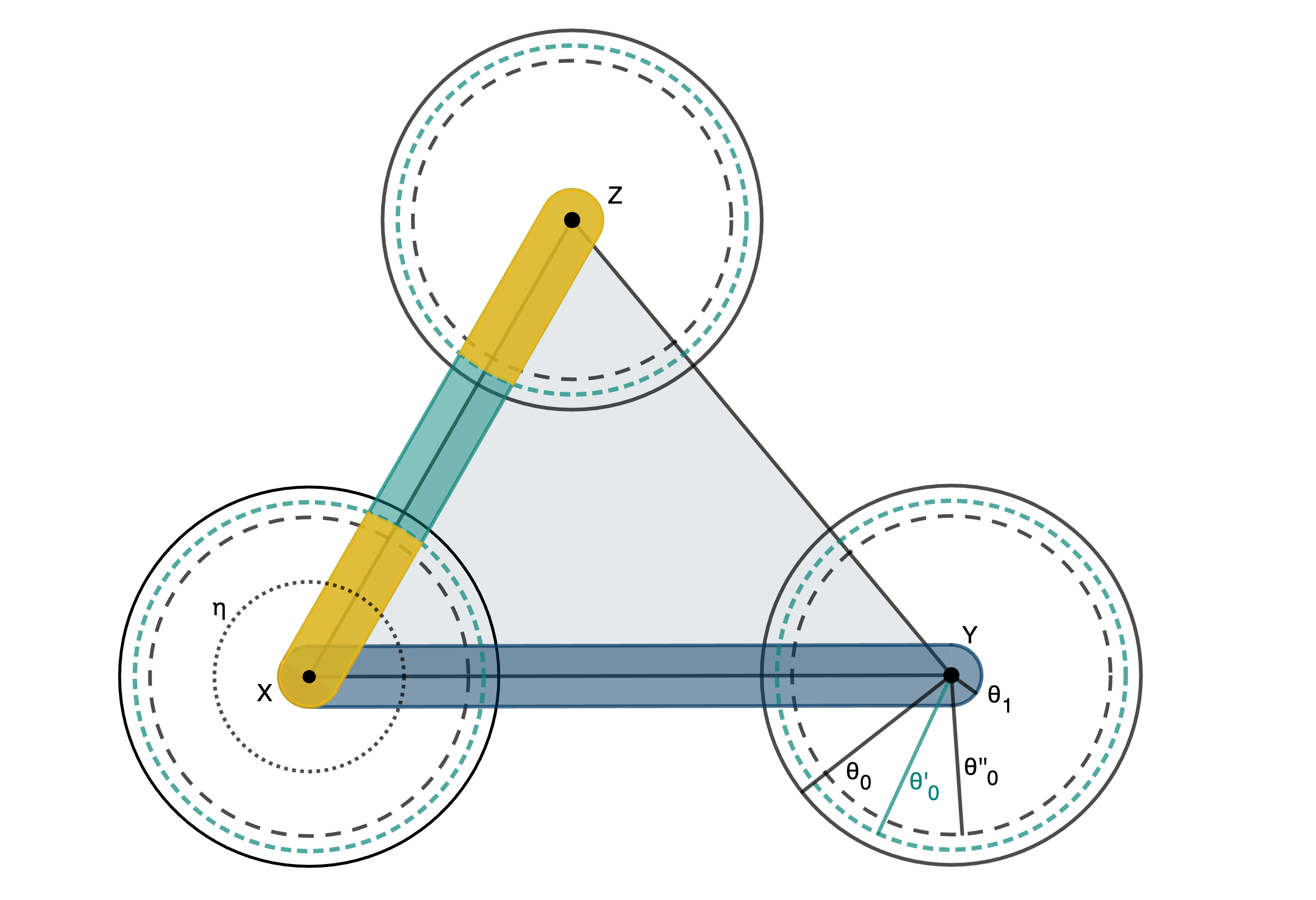
Figure 1. When perturbing the Delaunay set in the $\theta_{1}$-neighborhood of the $1$-cell $XZ$, the points in the $r$-neighborhood of the yellow zones are generic by induction, and so these points will not change when we apply the extended algorithm to this neighborhood. In particular, since the $\theta_{1}$-neighborhoods of $XY$ and $XZ$ lie inside the ball $\eta$ of radius $\frac{\theta_{0}}{2}$, their Delaunay sets inside this intersection agree. These neighborhoods are far enough away outside of $\eta$ so that their union contains no degeneracy after applying the extended algorithm.

We begin with a lemma that will allow use to piece together nice Delaunay sets inductively. Given a smooth submanifold $S\subseteq\mathcal{M}$ and $t>0$, we let $N_{t}(S):=\left\{p\in\mathcal{M}\;\middle|\;d(p,S)<t\right\}$ denote the $t$-neighborhood around $S$. Unless otherwise specified, in what follows once we have selected some $\varepsilon>0$, we will use $r=r(\varepsilon):=10\varepsilon$ as in Theorem 3.1.

Lemma 4.2.

Let $\Delta\subseteq\mathcal{M}$ be a $C^{\infty}$ closed submanifold diffeomorphic to a closed $k$-disk for some $k\leq n$. Let $\frac{\theta_{k-1}}{2}\geq\theta_{k}>0$ be such that $N_{\theta_{k-1}}(\partial\Delta)$ and $N_{\theta_{k}}(\Delta)$ are tubular. Let $0<\varepsilon<\frac{\theta_{k}}{100}$ and suppose furthermore that $\varepsilon$ is small enough to satisfy the conditions of Theorem 3.1. Suppose that there is a generic Delaunay set $D_{\partial}$ of mesh $(\mu,\varepsilon)$ on $N_{\theta_{k-1}}(\partial\Delta)$. Then for $\theta_{k-1}^{\prime}:=\theta_{k-1}-r$ there is a generic Delaunay set $D_{\Delta}$ of mesh $(\mu,\varepsilon)$ on $N_{\theta_{k}}(\Delta)$ such that

$$D_{\Delta}\cap N_{\theta_{k-1}^{\prime}}(\partial\Delta)=D_{\partial}\cap N_{\theta_{k-1}^{\prime}}(\partial\Delta)\cap N_{\theta_{k}}(\Delta).$$ (4.1)

Proof.

Put an arbitrary Delaunay set $D$ on $N_{\theta_{k}}(\Delta)$ of mesh $(\mu,\varepsilon)$ which extends that of $D_{\partial}\cap N_{\theta_{k}}(\Delta)$. That is, the only constraint on $D$ is that

$$D\cap N_{\theta_{k-1}}(\partial\Delta)=D_{\partial}\cap N_{\theta_{k-1}}(\partial\Delta)\cap N_{\theta_{k}}(\Delta).$$

Put an enumeration on points inside of $N_{\theta_{k}}(\Delta)$ such that, whenever we have $x_{i}\in N_{\theta_{k-1}^{\prime}}(\partial\Delta)$ and $x_{j}\in N_{\theta_{k}}(\Delta)\setminus N_{\theta_{k-1}^{\prime}}(\partial\Delta)$ then $i\leq j$. We take this enumeration as part of the input to the extended algorithm referenced in Theorem 3.1.

Note: While it isn’t necessarily true that we have each $B_{r}(x_{i})$ a $(\mu,\varepsilon)$-net (say, near the boundary of $\overline{N_{\theta_{k}}(\Delta)}$), by restricting our enumeration further to $N_{\theta_{k}-r}(\Delta)$, and being careful to choose sufficiently small $r$ and sufficiently small $\varepsilon$ in the first place, while replacing the $\theta_{k}$-neighborhood with one of radius $\theta_{k}-2r$, or else simply expanding to a Delaunay set on a slightly larger ball, this does not pose a problem. This is essentially the act of restricting our attention to "safe interior points" as described in [2].

Now, we apply Theorem 3.1 to create a generic Delaunay set $D_{\Delta}$ which is a small perturbation of $D$. It remains to show that $D_{\Delta}$ satisfies (4.1). However, as the algorithm "proceeds by perturbing each point…in turn, such that each point is only visited once" (see [3, p.4]), we perturb the points according to the enumeration placed on the input Delaunay set.

In particular, the points in $D\cap N_{\theta_{k-1}^{\prime}}(\partial\Delta)$ are visited first. However, relative to their neighbors up to a ball of radius $r$, such points are already in generic position. Thus, the perturbation algorithm leaves these points unchanged. (In Figure 1, for example, the points in the yellow zone remain static when adjusting the Delaunay set around the $1$-cell $XZ$.) Therefore, since $\theta_{k-1}^{\prime}<\theta_{k-1}$ we have the required equality:

$$D_{\Delta}\cap N_{\theta_{k-1}^{\prime}}(\partial\Delta)=D\cap N_{\theta_{k-1}^{\prime}}(\partial\Delta)\\ =D_{\partial}\cap N_{\theta_{k-1}^{\prime}}(\partial\Delta)\cap N_{\theta_{k}}(\Delta).$$

∎

Corollary 4.3.

Suppose that $\Delta$ and $\Delta^{\prime}$ are two $k$-disks satisfying the conditions of the above lemma for uniform choices of $\theta_{k-1}$ and $\theta_{k}$ and $\varepsilon$. Suppose moreover that $\Delta\cap\Delta^{\prime}\subseteq\partial\Delta$ is a closed $(k-1)$-disk with

$$D_{\partial}\cap N_{\theta_{k-1}}(\Delta\cap\Delta^{\prime})=D_{\partial^{\prime}}\cap N_{\theta_{k-1}}(\Delta\cap\Delta^{\prime}).$$ (4.2)

Suppose furthermore that, for $\theta_{k-1}^{\prime\prime}=\theta_{k-1}^{\prime}-r=\theta_{k-1}-2r$ we have

$$N_{\theta_{k}}(\Delta)\cap N_{\theta_{k}}(\Delta^{\prime})\subseteq N_{\theta_{k-1}^{\prime\prime}}(\Delta\cap\Delta^{\prime})$$ (4.3)

and that $N_{\theta_{k}}(\Delta)$ and $N_{\theta_{k}}(\Delta^{\prime})$ are separated by some distance greater than $5r$ outside of $N_{\theta_{k-1}^{\prime\prime}}(\Delta\cap\Delta^{\prime})$.

Then for $D_{\Delta}$ and $D_{\Delta^{\prime}}$ as given by the lemma,

$$D_{\Delta}\cap N_{\theta_{k-1}^{\prime}}(\Delta\cap\Delta^{\prime})\cap N_{\theta_{k}}(\Delta^{\prime})=D_{\Delta^{\prime}}\cap N_{\theta_{k-1}^{\prime}}(\Delta\cap\Delta^{\prime})\cap N_{\theta_{k}}(\Delta)$$

and $D_{\Delta}\cup D_{\Delta^{\prime}}$ is a generic Delaunay set on $N_{\theta_{k}}(\Delta)\cup N_{\theta_{k}}(\Delta^{\prime})$.

Proof.

First, conjugating an application of (4.2) by applications of 4.2, we have

$$D_{\Delta}\cap N_{\theta_{k-1}^{\prime}}(\Delta\cap\Delta^{\prime})\cap N_{\theta_{k}}(\Delta^{\prime}) =D_{\partial}\cap N_{\theta_{k-1}^{\prime}}(\Delta\cap\Delta^{\prime})\cap N_{\theta_{k}}(\Delta)\cap N_{\theta_{k}}(\Delta^{\prime})$$

$$=D_{\partial^{\prime}}\cap N_{\theta_{k-1}^{\prime}}(\Delta\cap\Delta^{\prime})\cap N_{\theta_{k}}(\Delta)\cap N_{\theta_{k}}(\Delta^{\prime})$$

$$=D_{\Delta^{\prime}}\cap N_{\theta_{k-1}^{\prime}}(\Delta\cap\Delta^{\prime})\cap N_{\theta_{k}}(\Delta).$$

Now to see that $D_{\Delta}\cup D_{\Delta^{\prime}}$ is generic, it suffices to check this on points of $D_{\Delta}$ which are near to those of $D_{\Delta^{\prime}}$. However, such degeneracy may only occur if points are with distance $r$ of each other. In particular, then, such a degeneracy may only occur in an $r$-ball of a point inside $N_{\theta_{k}}(\Delta)\cap N_{\theta_{k}}(\Delta^{\prime})\subseteq N_{\theta_{k-1}^{\prime\prime}}(\Delta\cap\Delta^{\prime})$ as points are separated by distance $5r$ otherwise. The above equalities show, however, that such a degeneracy would be contained in an $r$-ball within the set

$$(D_{\Delta}\cup D_{\Delta^{\prime}})\cap N_{\theta_{k}}(\Delta)\cap N_{\theta_{k}}(\Delta^{\prime}) \subseteq(D_{\Delta}\cup D_{\Delta^{\prime}})\cap N_{\theta_{k}}(\Delta)\cap N_{\theta_{k}}(\Delta^{\prime})\cap N_{\theta_{k-1}^{\prime}}(\Delta\cap\Delta^{\prime})$$

$$\subseteq D_{\partial}\cap N_{\theta_{k-1}}(\Delta\cap\Delta^{\prime}).$$

As this last set is generic, no such degeneracy can occur. ∎

Corollary 4.4.

Under the assumptions of 4.2, the triangulation induced by $D$ in $N_{\theta_{k}}(\Delta)$ agrees with that of $D_{\partial}$ in $N_{\theta_{k-1}}(\partial\Delta)$ on the set $N_{\theta_{k-1}^{\prime\prime}}(\partial\Delta)$.

Proof.

Since the Delaunay sets agree in $N_{\theta_{k-1}^{\prime}}(\partial\Delta)$, the triangulation remains unchanged except perhaps within the $r$-neighborhood of the boundary of $N_{\theta_{k-1}^{\prime}}(\partial\Delta)$. ∎

We now return our attention to the context of tilings.

Lemma 4.5.

For each $k\leq n$, there is a $\theta_{k}>0$ such that $\theta_{k}\leq\frac{\theta_{k-1}}{2}$, and for any $k$-cell $\Delta$ of a prototile $P$, we have $N_{\theta_{k}}(\Delta^{int})$ a tubular neighborhood. Furthermore, if $\Delta^{\prime}$ is a $j$-cell ($j\leq k$) then

$$N_{\theta_{k}}(\Delta)\cap N_{\theta_{k}}(\Delta^{\prime})\subseteq N_{\theta_{k-1}/2}(\Delta\cap\Delta^{\prime}),$$ (4.4)

and otherwise these neighborhoods are separated by distance $\geq\theta_{k}$.

Proof.

Inductively assume that such a $\theta_{k-1}>0$ exists. Let $\Delta$ be a $k$-cell of a prototile $P$. By normality $\Delta$ is a (piecewise) smooth submanifold diffeomorphic to a closed topological disk. Thus there is some $\tau_{P,\Delta}>0$ such that $N_{\tau_{P,\Delta}}(\Delta^{int})$ is tubular in $\mathcal{M}$. Since there are finitely many prototiles, and finitely many cells of dimension $k$, set $\tau_{k}:=\min_{P,\Delta}\left\{\tau_{P,\Delta}\right\}$, and observe that $\tau_{k}>0$.

Now, let $\Delta^{\prime}$ be any other $j$-cell of $P$, where $j\leq k$. If $\Delta\cap\Delta^{\prime}=\emptyset$, then they are separable by some $R_{P,\Delta,\Delta^{\prime}}>0$. If $\Delta\cap\Delta^{\prime}\neq\emptyset$, then their intersection is a $b$-cell $\beta\subseteq\partial\Delta$ for some $b\leq\min\left\{j,k-1\right\}$. Therefore, there is some radius $R_{P,\Delta,\Delta^{\prime}}>0$ separating $\Delta$ and $\Delta^{\prime}$ outside a small neighborhood of $\beta$. In particular, we select $R_{P,\Delta,\Delta^{\prime}}>0$ so that

$$d\left(\Delta\setminus N_{\theta_{b}}(\beta)\;,\;\Delta^{\prime}\setminus N_{\theta_{b}}(\beta)\right)>R_{P,\Delta,\Delta^{\prime}}.$$ (4.5)

Observe that $N_{\theta_{b}}(\beta)$ is tubular by induction. Furthermore, we see that $R_{P,\Delta,\Delta^{\prime}}\leq 2\theta_{b}$ since $\Delta\cap\Delta^{\prime}=\beta$. Consequently $\frac{R_{P,\Delta,\Delta^{\prime}}}{4}\leq\frac{\theta_{b}}{2}$ and hence

$$N_{\frac{R_{P,\Delta,\Delta^{\prime}}}{4}}(\Delta)\cap N_{\frac{R_{P,\Delta,\Delta^{\prime}}}{4}}(\Delta^{\prime})\subseteq N_{\theta_{b}/2}(\beta)=N_{\theta_{b}/2}(\Delta\cap\Delta^{\prime}).$$ (4.6)

As there are only finitely many prototiles, and finitely many cells of dimension $\leq k$ in each prototile, we set $R_{k}:=\min_{P}\left\{R_{P,\Delta,\Delta^{\prime}}\;\middle|\;\dim(\Delta^{\prime})\leq\dim(\Delta)=k\right\}$, and we have $R_{k}>0$.

Finally, we set $\theta_{k}=\min\left\{\tau_{k},\frac{R_{k}}{4},\frac{\theta_{k-1}}{2}\right\}$. By definition of $\tau_{k}$, we have the tubular neighborhood requirement on every $k$-cell of every prototile. Furthermore, as equation (4.6) holds on all prototiles and all relevant choices of $\Delta$ and $\Delta^{\prime}$ in any prototile $P$, the condition (4.4) holds as well. By (4.5), the separability condition on $\theta_{k}$-neighborhoods away from intersections holds as well. It is clear that $\theta_{k}\leq\frac{\theta_{k-1}}{2}$. ∎

Corollary 4.6.

If $r<\frac{\theta_{k-1}}{10}$, then under the setup of the above lemma,

$$N_{\theta_{k}}(\Delta)\cap N_{\theta_{k}}(\Delta^{\prime})\subseteq N_{\theta_{k-1}^{\prime\prime}}(\Delta\cap\Delta^{\prime})$$

and otherwise they are separated by distance $\geq 10r>5r$.

Lemma 4.7.

Let $\left\{\theta_{0},\dots,\theta_{n}\right\}$ be as guaranteed by the previous lemma. Let $0<\varepsilon<\frac{\theta_{n}}{100}$. There is a generic Delaunay set $D_{P}$ of mesh $(\mu,\varepsilon)$ on each collared prototile $P$, such that if $T=g.P$ and $T^{\prime}=g^{\prime}.P^{\prime}$ are tiles in a tiling $\mathcal{T}$ with $T\cap T^{\prime}=\beta$, then $D_{T}\cup D_{T^{\prime}}$ is generic and

$$D_{T}\cap N_{\theta_{n}}(T\cap T^{\prime})=D_{T^{\prime}}\cap N_{\theta_{n}}(T\cap T^{\prime})$$

where $D_{T}:=g.D_{P}$ and $D_{T^{\prime}}:=g^{\prime}.D_{P^{\prime}}$. In particular $D_{T}$ depends only on the collar of $P$, and is independent of the collar of $P^{\prime}$.

Proof.

Inductively, suppose that we have defined a Delaunay set $D_{P,k-1}$ of mesh $(\mu,\varepsilon)$ on each collared prototile $P$ such that the following two conditions hold:

1. $D_{P,k-1}\cap N_{\theta_{k-1}}(\bigcup_{\beta}\beta)$ is generic for any finite union of $(k-1)$-cells $\beta\subseteq P$.

2. Suppose $T=g.P$ and $T^{\prime}=g^{\prime}.P^{\prime}$ are tiles with $T\cap T^{\prime}=\beta$ for some cell $\beta$ of dimension $\leq k-1$. Let $D_{T,k-1}=g.D_{P,k-1}$ and $D_{T^{\prime},k-1}=g^{\prime}.D_{P^{\prime},k-1}$. Then

   $$D_{T,k-1}\cap N_{\theta_{k-1}}(\beta)=D_{T^{\prime},k-1}\cap N_{\theta_{k-1}}(\beta).$$

   In other words,

   $$D_{P,k-1}\cap N_{\theta_{k-1}}(\beta)\sim_{G}D_{P^{\prime},k-1}\cap N_{\theta_{k-1}}(\beta).$$

   where we abuse notation and write $\beta$ here to mean the copy of $\beta$ showing up in $P$ and $P^{\prime}$ respectively.

Let $\widetilde{\Delta}$ be a $k$-cell in $\Gamma$. By hypothesis, if $\Delta$ is a copy of $\widetilde{\Delta}$ living in a collared prototile $P$, then there is an induced Delaunay set $D_{\partial}$ defined on $N_{\theta_{k-1}}(\partial\Delta)$. Furthermore, condition (2) means that $D_{\partial}$ is (by induction) independent of the collared prototile chosen. More precisely, if $\Delta$ shows up as a $k$-cell in two different collared prototiles $P$ and $P^{\prime}$, then up to the action of $G$,

$$D_{P,k-1}\cap N_{\theta_{k-1}}(\partial\Delta)\sim_{G}D_{P^{\prime},k-1}\cap N_{\theta_{k-1}}(\partial\Delta).$$

By 4.2 there is a generic Delaunay set $D_{\Delta}$ of mesh $(\mu,\varepsilon)$ on $N_{\theta_{k}}(\Delta)$ such that

$$D_{\Delta}\cap N_{\theta_{k-1}^{\prime}}(\partial\Delta)=D_{\partial}\cap N_{\theta_{k-1}^{\prime}}(\partial\Delta)\cap N_{\theta_{k}}(\Delta).$$

Given a collared prototile $P$ for which $\Delta$ shows up as a $k$-cell, define a Delaunay set on $N_{\theta_{k}}(\Delta)$ by $D_{P,k,\Delta}:=D_{\Delta}$. Then if $g.P\cap g^{\prime}.P^{\prime}\subseteq\Delta$, clearly

$$D_{P,k,\Delta}=D_{\Delta}\sim_{G}D_{P^{\prime},k,\Delta}.$$ (4.7)

We define $D_{P,k}:=\bigcup_{\Delta}D_{P,k,\Delta}$. Note that if $\Delta$ and $\Delta^{\prime}$ are two $k$-cells of $P$, then $N_{\theta_{k}}(\Delta)$ and $N_{\theta_{k}}(\Delta^{\prime})$ are separated by distance $5r$ outside of $N_{\theta_{k-1}^{\prime\prime}}(\Delta\cap\Delta^{\prime})$ by 4.6. By 4.3, therefore, the finite union $D_{P,k}$ is generic in the $\theta_{k}$-neighborhood of any finite union $k$-cell. Extend each $D_{P,k}$ outside the $\theta_{k}$-neighborhood of $k$-cells arbitrarily to be a Delaunay set on all of $P$, also denoted $D_{P,k}$. This completes the inductive step.

The inductive process ends at $k=n$, completing the proof. ∎

The main result follows now without much trouble.

Proof of Section 1.

On each collared prototile, fix a Delaunay set as given by 4.7. This induces a point set on $\Gamma$, which pulls back to the original tiling. By construction, the Delaunay set on any collared tile is the Delaunay set on the corresponding collared prototile, hence is generic with respect to the Delaunay sets of neighboring tiles. This induces a triangulation (as in 4.4) which is compatible between tiles.

In particular, the neighborhood of radius $\theta_{n}^{\prime\prime}=\theta_{n}-2r$ of any collared prototile uniquely determines the Delaunay triangulation of that collared prototile so that it glues onto the triangulation of neighboring tiles. This process is obviously reversible by careful labelling of the Delaunay simplices, and the triangulation is MLD to the original tiling. ∎

5. Nilpotent Lie Groups

In this section, we present the background on nilpotent Lie groups, paying special attention to connected, simply connected, rational, nilpotent Lie groups with a left-invariant Riemannian metric. The reader familiar with such groups is welcome to skip this section, except perhaps as reference for future notation.

5.1. Notation and Foundations

First, a (real) Lie group is a (real) smooth manifold with a compatible group structure, by which we mean that the actions of multiplication and inversion are smooth diffeomorphisms of the manifold. The tangent spaces of a Lie group $G$ can therefore all be identified by left-translation with the tangent space $\mathfrak{g}=T_{e}G$ at the identity, which we call the Lie algebra of $G$. There is a place for discussing the rich theory of Lie algebras in their own right, but for now we simply make the comment that the lie algebra $\mathfrak{g}$ associated to $G$ is a vector space together with an alternating bilinear map $[\cdot,\cdot]:\mathfrak{g}\times\mathfrak{g}\to\mathfrak{g}$ called the lie bracket. Furthermore, for any $x\in G$ there is an important map $\exp_{x}:\mathfrak{g}\to G$ for which $\exp_{x}(0)=x$, called the exponential map at $x$. For connected, simply connected nilpotent lie groups/lie algebras, we will recall in 5.1 that this map in fact induces a diffeomorphism $\mathfrak{g}\simeq G$.

A nilpotent group can be thought of a one which is, in some sense, "almost abelian". Let $G$ be a group. Recall that for $x,y\in G$, we define the commutator $[x,y]:=xyx^{-1}y^{-1}$, and for subgroups $H,K$ of $G$ we define $[H,K]:=\left\{[h,k]\;\middle|\;h\in H,k\in K\right\}$. We define $G_{0}:=G$, and inductively for $n>0$, we set $G_{n}:=[G_{n-1},G]$. These subgroups fit together into a lower central series:

$$G=G_{0}\unrhd G_{1}\unrhd G_{2}\unrhd\cdots\unrhd G_{n}\unrhd\cdots$$

In the event that $G_{s}=\left\{e\right\}$ for some $s\in\mathbb{N}$, we say that the series terminates, and that the group $G$ is nilpotent. The smallest $s$ for which $G_{s}=\left\{e\right\}$ is called the nilpotency step or nilpotency class of $G$. Observe that if $s=1$, the group $G$ is abelian.

In our context, we will say that a connected, simply connected Lie group is a nilpotent Lie group if it is nilpotent as a group. However, we can also relate the notion of nilpotency to the Lie algebra $\mathfrak{g}$. In fact, we define $L_{0}:=\mathfrak{g}$ and inductively define subspaces $L_{n}:=[L_{n-1},L]$ where the bracket here is the Lie bracket of $\mathfrak{g}$. These again fit into a lower central series

$$\mathfrak{g}=L_{0}\supseteq L_{1}\supseteq L_{2}\supseteq\cdots\supseteq L_{n}\supseteq\cdots$$

In the event that $L_{s}=\left\{0\right\}$ for some $s\in\mathbb{N}$, we say that the series terminates, and that the lie algebra $\mathfrak{g}$ is nilpotent. The smallest $s$ for which $L_{s}=\left\{0\right\}$ is called the nilpotency step or nilpotency class of $\mathfrak{g}$. Observe that if $s=1$, the Lie bracket $[\cdot,\cdot]$ is trivial, and $\mathfrak{g}=\mathbb{R}^{n}$ as an abelian Lie algebra.

The following proposition is classical and can be found in many reasonable textbooks on the theory of Lie groups (for example, see [6, Sec. 1.2]).

Proposition 5.1.

If $G$ is a connected, simply connected nilpotent lie group, then $\exp_{e}:\mathfrak{g}\to G$ is a diffeomorphism.

Often a nilpotent Lie group is defined to be one whose Lie algebra is nilpotent. In our context, the group (and not the algebra) structure will be our main focus, and so we take the nilpotence of $G$ for granted, stating the following as a proposition.

Proposition 5.2.

Let $G$ be a connected, simply connected Lie group. Then $\mathfrak{g}$ is a nilpotent Lie algebra if and only if $G$ is a nilpotent Lie group.

The proofs of the above facts rely on what is commonly known as the BCH formula. This is a way of translating between the Lie bracket of $\mathfrak{g}$ and the group structure of $G$.

Theorem 5.3 (BCH Formula).

Let $X,Y\in\mathfrak{g}$. Then $\exp(X)\cdot\exp(Y)=\exp(Z)$ where

$$Z=X+Y+\frac{1}{2}[X,Y]+\frac{1}{12}\left([X,[X,Y]]+[Y,[Y,X]]\right)+\cdots$$

where "higher order" terms are successive nestings of commutators of $X$ and $Y$.

Note that in a nilpotent Lie group, since successive commutators eventually vanish. Therefore the BCH formula is a finite sum in this context and hence always terminates. We note that the BCH formula has been fruitful in the study of nilpotent tilings already—for example, see [8].

From now on, unless otherwise specified, all Lie groups will be assumed to be connected, simply connected, and nilpotent. We will use $\mathbb{G}$ (rather than $G$) to denote such a group, and though we may frequently remind the reader that $\mathbb{G}$ is assumed to be nilpotent, we will not typically mention that $\mathbb{G}$ is connected and simply connected.

5.2. The Heisenberg Group

The first example of a non-abelian nilpotent Lie group is the $3$-dimensional Heisenberg group $\mathbb{H}(\mathbb{R})=\mathbb{H}^{3}=\mathbb{H}$. This is commonly viewed as the upper triangular matrix Lie group with $1$’s along the diagonal:

$$\mathbb{H}=\left\{\begin{pmatrix}1&x&z\\ 0&1&y\\ 0&0&1\end{pmatrix}\;\middle|\;x,y,z\in\mathbb{R}\right\}.$$

Alternatively, we view this group as $\mathbb{R}^{3}$ with the non-abelian group law

$$(x,y,z)\star(x^{\prime},y^{\prime},z^{\prime})=(x+x^{\prime},y+y^{\prime},z+xy^{\prime}+z^{\prime}).$$

This group is $2$-step nilpotent with center $Z(\mathbb{H})=\left\{(0,0,z)\;\middle|\;z\in\mathbb{R}\right\}$ and commutator subgroup $[\mathbb{H},\mathbb{H}]=\left\{(x,y,0)\;\middle|\;x,y\in\mathbb{R}\right\}$. It is easily seen that $\mathbb{H}(\mathbb{Z}):=\left\{(x,y,z)\;\middle|\;x,y,z\in\mathbb{Z}\right\}$ and $\mathbb{H}(\mathbb{Q}):=\left\{(x,y,z)\;\middle|\;x,y,z\in\mathbb{Q}\right\}$ are subgroups of $\mathbb{H}$. They are (respectively) the integer and rational Heisenberg groups. Observe that in these definitions, we readily apply exponential coordinates.

The Lie algebra $\mathfrak{h}$ of $\mathbb{H}$ is generated by basis $\left\{X,Y,Z\right\}$ with $\exp_{e}(X)=x=(1,0,0)$, and $\exp_{e}(Y)=y=(0,1,0)$, and $\exp_{e}(Z)=z=(0,0,1)$. The Lie bracket satisfies $[X,Y]=Z$, with all other brackets being trivial.

5.3. Rational Lie Groups

To prove Section 1, we will need to consider a class of Lie groups known as rational Lie groups.

Definition 5.4.

Let $\mathbb{G}$ be a real nilpotent Lie group. We say that $\mathbb{G}$ is rational if there is a basis $\left\{X_{1},\dots,X_{n}\right\}$ of the Lie algebra $\mathfrak{g}$ whose structure coefficients are in $\mathbb{Q}$. That is, the bracket relations satisfy $[X_{i},X_{j}]=\sum_{k}c_{i,j,k}X_{k}$ where $c_{i,j,k}\in\mathbb{Q}$.

A celebrated theorem by Malcev explains that such rational Lie groups are precisely those admitting lattices:

Theorem 5.5 (Malcev’s Correspondence, [15]).

A connected, simply connected, nilpotent Lie group $\mathbb{G}$ is rational if and only if $\mathbb{G}$ has a lattice.

Here, a (cocompact) lattice of $\mathbb{G}$ is a discrete subgroup $\Lambda$ for which $\mathbb{G}/\Lambda$ is compact. The quotient of a connected, simply connected, nilpotent Lie group $\mathbb{G}$ by a cocompact lattice $\Lambda$ is called a nilmanifold. For example, it can be shown that the integer points $\mathbb{H}(\mathbb{Z})$ form a lattice in $\mathbb{H}$. The nilmanifold $\mathbb{H}/\mathbb{H}(\mathbb{Z})$ is called the Heisenberg manifold.

Given a rational nilpotent Lie group $\mathbb{G}$, we call a lattice integral or an integer lattice when the lattice has integral exponential coordinates. Such a lattice always exists for a rational nilpotent Lie group, and we will denote any such lattice by $\mathbb{G}(\mathbb{Z})$. Similarly, the set of rational points of $\mathbb{G}$ will be denoted by $\mathbb{G}(\mathbb{Q})$. This is the set of points whose coordinates are rational under exponential coordinates.

We will later require the following "folklore" lemma about the abundance of lattices of arbitrarily small covolume in rational, nilpotent Lie groups, a proof of which may be found in [5, Lemma 4.1].

Proposition 5.6.

Let $L$ be a cocompact discrete subring in $\mathfrak{g}$ for $\mathbb{G}$ a rational nilpotent Lie group. Then there are lattices $\Lambda_{1},\Lambda_{2}\subseteq\mathbb{G}$ with $[\Lambda_{2}:\Lambda_{1}]$ of finite index depending on $\dim(\mathfrak{g})$ for which $\Lambda_{1}\subseteq\exp(L)\subseteq\Lambda_{2}$.

As a consequence of this, we record the following corollary for later use.

Corollary 5.7.

Let $\mathfrak{S}\subseteq\mathfrak{g}$ be a finite set with rational coordinates such that $\mathrm{span}_{\mathbb{R}}(\mathfrak{S})=\mathfrak{g}$. Then there is a lattice $\Lambda\subseteq\mathbb{G}$ such that $\langle S\rangle\subseteq\Lambda$, where $S:=\exp(\mathfrak{S}):=\left\{\exp(s_{i})\;\middle|\;s_{i}\in\mathfrak{S}\right\}$.

Proof.

As the coordinates of $\mathfrak{S}$ are all rational, an application of the BCH formula implies that there is a cocompact discrete subring $L$ in $\mathfrak{g}$ containing $\mathfrak{S}$ (say, the Lie subring generated by basis vectors scaled by the greatest common divisor of coordinates from $\mathfrak{S}$). Thus $\exp(L)$ contains $S$. Taking $\Lambda=\Lambda_{2}$ from the above proposition, we see that $\langle S\rangle\subseteq\Lambda$ as claimed. ∎

5.4. Left-Invariant Metrics

With 5.1 in mind, we can (and in many ways, we should) view connected, simply connected, nilpotent Lie groups as a copy of $\mathbb{R}^{n}$ with a non-abelian group law. This perspective warrants some caution: the Euclidean metric on $\mathbb{R}^{n}$ will not behave well with respect to a non-abelian group law. It is therefore natural to equip our group with a metric more naturally associated to this group structure.

For an arbitrary group $G$, a left-invariant distance on $G$ is a metric $d:G\times G\to G$ such that, for any $a,q_{1},q_{2}\in G$, we satisfy $d(aq_{1},aq_{2})=d(q_{1},q_{2})$. Associated to any Lie group is a family of left-invariant Riemannian metrics, each of which naturally induce a left-invariant distance. In what follows, we will assume that our nilpotent Lie group has such a left-invariant Riemannian metric.

Once a left-invariant Riemannian metric has been set on $G$, we get that $G$ is homogeneous: anything that we want to know about the local geometry of $G$ around a point $a\in G$ can be determined by considering $e\in G$ instead. For example, Section 1 applies to tilings of $\mathbb{G}$.

6. Tiling Spaces are Cantor Set Fiber Bundles

Throughout this section, we fix a simple tiling space $\mathscr{T}$ of a connected, simply connected, rational, nilpotent Lie group $\mathbb{G}$. The vertices are therefore assumed to form a generic $(\mu,\varepsilon)$-net on $r$-balls where (as before) $r=10\varepsilon$. The goal of this section is Section 1, providing evidence that other theorems on simple tilings of $\mathbb{R}^{n}$ may be naturally generalized to the context of simple tilings of nilpotent Lie groups.

Given a prototile $P$, we have seen that we can think of the vertex set as abstracting away the particular geometry of the tiles, allowing us to describe the combinatorics by the points in a small ball around any given vertex. The star of any vertex in a tiling may be assumed to embed into the Gähler complex $\Gamma$, and thus all of the relevant combinatorics and geometry will be legible from $\Gamma$ alone. We introduce shape functions as a natural way to read this information.

Definition 6.1.

A shape function for $\mathscr{T}$ is a $\mathbb{G}$-valued $1$-cocycle $s\in Z^{1}(\Gamma,\mathbb{G})=\operatorname{ker}\left(\delta_{1}\right)$. That is, $\delta_{1}(s)\equiv e$, so in particular, if $w$ is a $2$-cell of $\Gamma$, then $s(\partial_{2}w)=e$.

We often will write $\delta$ in place of $\delta_{1}$ and $\partial$ in place of $\partial_{2}$. Observe that a priori, shape functions are defined fairly generally. There is no reference to the exact geometry of tilings in $\mathscr{T}$, nor are there any obvious combinatorics from this tiling space in play. We would like to have a shape function which encodes this relevant information for our particular tiling space $\mathscr{T}$, and the first task is to provide such a function.

Definition 6.2.

Let $P$ be a prototile, and let $E$ be an oriented edge of $P$ from $x$ to $y$. Let $\widetilde{E}:=\pi(E)$ be the embedding of $E$ into $\Gamma$. The displacement of $E$ is defined to be $d(\widetilde{E}):=x^{-1}y$.

Observe that this is well-defined, independent of choice of prototile $P$ containing $E=\pi_{P}^{-1}(\widetilde{E})$. To be sure, suppose that $P^{\prime}$ were another such tile containing $E^{\prime}=\pi^{-1}_{P^{\prime}}(\widetilde{E})$ from $u$ to $v$. Let $d(\widetilde{E}^{\prime})$ denote the displacement of the edge computed in $P^{\prime}$ rather than $P$. By definition of $\Gamma$ there would be some left-translates of $P$ and $P^{\prime}$ such that the translated tiles meet along the (translated) edge $E$. This means in particular that there is a $g\in\mathbb{G}$ for which $x=gu$ and $y=gv$ so that

$$d(\widetilde{E})=x^{-1}y=(gu)^{-1}(gv)=u^{-1}v=d(\widetilde{E}^{\prime}).$$

Definition 6.3.

Let $s_{\mathscr{T}}\in C^{1}(\Gamma,\mathbb{G})$ be defined on (oriented) edges by $s_{\mathscr{T}}(E)=d(E)$, and by concatenation otherwise. We call $s_{\mathscr{T}}$ the shape function associated to $\mathscr{T}$.

It is appropriate to justify such an evocative name:

Proposition 6.4.

The shape function associated to $\mathscr{T}$ is a shape function.

Proof.

Without loss of generality, say by appropriate labeling of our tiles in the first place (or by a sufficiently fine subdivision process), we can assume that the projection $\pi:\mathcal{T}\to\Gamma$ is an embedding on any tile $T\subseteq\mathcal{T}$. In particular, the boundary of any single $2$-cell in $\Gamma$ corresponds exactly to the boundary of a $2$-cell of some collared prototile.

This means that if $\widetilde{w}$ is a $2$-cell in $\Gamma$, then, there is a $2$-cell $w$ in some prototile $P$ for which $\pi_{P}(w)=\widetilde{w}$ is an embedding. Suppose that $\partial\widetilde{w}=\widetilde{E}_{1}\widetilde{E}_{2}\cdots\widetilde{E}_{k}$. Then $\partial w=E_{1}E_{2}\cdots E_{k}$ where $\pi_{P}(E_{j})=\widetilde{E_{j}}$ for each $1\leq j\leq k$. Let the edge $E_{j}$ be directed from the vertex $v_{j-1}$ to the vertex $v_{j}$. Then

$$(\delta s_{\mathscr{T}})(\widetilde{w}) =s_{\mathscr{T}}(\partial\widetilde{w})$$

$$=s_{\mathscr{T}}(\widetilde{E}_{1})\cdot s_{\mathscr{T}}(\widetilde{E}_{2})\cdots s_{\mathscr{T}}(\widetilde{E}_{k})$$

$$=d(\widetilde{E}_{1})\cdot d(\widetilde{E}_{2})\cdots d(\widetilde{E}_{k})$$

$$=(v_{0}^{-1}v_{1})\cdot(v_{1}^{-1}v_{2})\cdot\cdots\cdot(v_{k-1}^{-1}v_{k})$$

$$=v_{0}^{-1}v_{k}$$

$$=e.$$

The final equality holds since $w$ is a $2$-cell whose boundary is $E_{1}E_{2}\cdots E_{k}$, so that $v_{k}=v_{0}$. Since the set of $2$-cells provides a basis for $C_{2}(\Gamma)$, we see that $s_{\mathscr{T}}\in\operatorname{ker}\left(\delta\right)$ is a shape function. ∎

Note.

From now on, given a shape function $\sigma$, we will often write $\sigma(E)$ rather than $\sigma(\widetilde{E})$ for a particular edge $E$ occurring in a particular prototile (or even a particular tile).

Suppose now that $\sigma\in Z^{1}(\Gamma,\mathbb{G})$ is a shape function for $\mathscr{T}$. It is possible that $\sigma$ is not the shape function associated to $\mathscr{T}$. Under what circumstances will $\sigma$ be the shape function associated to some tiling space $\mathscr{T}_{\sigma}$? When this is the case, how are $\mathscr{T}$ and $\mathscr{T}_{\sigma}$ related? Under what circumstances will $\mathscr{T}$ and $\mathscr{T}_{\sigma}$ be equivalent (and under which version of equivalence)?

We show below that ${\sigma}$ will induce a new tiling space $\mathscr{T}_{\sigma}$ as long as $d(s_{\mathscr{T}}(E),\sigma(E))$ is small enough for every edge $E$. In particular, since the Delaunay set associated to our tilings are $\delta$-generic, the combinatorics of the tiles are invariant under small enough $\varrho$-perturbations. We therefore ask that $d(s_{\mathscr{T}}(E),\sigma(E))<\varrho$, and when this is the case 6.7 below demonstrates that a tiling space $\mathscr{T}_{\sigma}$ exists whose associated shape function is $\sigma$, and in fact $\mathscr{T}_{\sigma}$ is homeomorphic to $\mathscr{T}$.

Note.

We cannot make $d(s_{\mathscr{T}}(E),\sigma(E))$ small enough to expect that $\mathscr{T}$ and $\mathscr{T}_{\sigma}$ are topologically conjugate, let alone MLD. For example, suppose that $s_{\mathscr{T}}$ describes the hull of a periodic tiling of $\mathbb{R}^{2}$ by squares of unit side length, and let $\sigma$ be arbitrarily close to $s_{\mathscr{T}}$, but describing squares of irrational side length. Even though the hulls $\mathscr{T}$ and $\mathscr{T}_{\sigma}$ corresponding to each of these tilings are homeomorphic tori, the action of $\mathbb{Z}^{2}$ on the tiling space $\mathscr{T}$ is periodic, but would be evidently aperiodic on $\mathscr{T}_{\sigma}$.

Proposition 6.5.

Let $\mathscr{T}$ be a simple tiling space with associated shape function $s_{\mathscr{T}}$. There is a $\varrho>0$ such that if $\sigma\in Z^{1}(\Gamma,\mathbb{G})$ with $d(s_{\mathscr{T}}(\widetilde{E}),\sigma(\widetilde{E}))<\varrho$ for each edge $\widetilde{E}$ of $\Gamma$, then for every prototile $P$, there is a corresponding $P^{(\sigma)}$ and a homeomorphism $\varphi_{P}:P\to P^{(\sigma)}$ such that if $P$ and $P^{\prime}$ are prototiles which meet along a common $k$-simplex $F$ in a tiling of $\mathscr{T}$, then $\varphi_{P}|_{F}$ agrees with $\varphi_{P^{\prime}}|_{F}$ up to translation.

Proof.

By assumption, the vertices of the prototiles of $\mathscr{T}$ are in generic position. Given a collared prototile $P$ with vertex $x$, we may assume without loss of generality (say, by taking a sufficiently large collar around $P$) that each simplex incident to $x$ is secure (see [2, Def. 3.11 & Lem. 4.10]). Let $\varrho_{x}$ be small enough to satisfy the conditions of Theorem 3.2 with $D=B_{r}(x)$, where we recall that $r=10\varepsilon$. We define $\varrho_{0}:=\min_{P\in\mathcal{P}}\left\{\varrho_{x}\;\middle|\;\text{$x$ is a vertex of $P$}\right\}$, and as there are finitely many prototiles, we have $\varrho_{0}>0$.

Set $\varrho<\frac{\varrho_{0}}{10}$ and suppose $\sigma$ is a shape function for $\mathscr{T}$ for which $d(s_{\mathscr{T}}(\widetilde{E}),\sigma(\widetilde{E}))<\varrho$ for each edge $\widetilde{E}$ of $\Gamma$. Given a prototile $P$, with vertices $\left\{x_{0},x_{1},\dots,x_{n}\right\}$, let $E_{i,j}$ be the edge from $x_{i}$ to $x_{j}$ for each $i\neq j$. Let $E_{j}:=E_{0,j}$. Define $x_{0}^{(\sigma)}:=x_{0}$, and for $j\neq 0$, let $x_{j}^{(\sigma)}:=\sigma(\widetilde{E}_{j})x_{0}^{(\sigma)}$.

Define a new prototile $P^{(\sigma)}$ to be the simplex whose vertices are $\left\{x_{0}^{(\sigma)},x_{1}^{(\sigma)},\dots,x_{n}^{(\sigma)}\right\}$. By Theorem 3.2, this simplex is uniquely determined by the vertex set. Furthermore, we show that up to left-translation, this definition of $P^{(\sigma)}$ is dependent only on $\sigma$, and not the particular enumeration of the vertices. Indeed, for any pair $i,j$ we have

$$(x_{i}^{(\sigma)})^{-1}x_{j}^{(\sigma)}=\left((x_{i}^{(\sigma)})^{-1}x_{0}^{(\sigma)}\right)\left((x_{0}^{(\sigma)})^{-1}x_{j}^{(\sigma)}\right)=\sigma(\widetilde{E}_{i})^{-1}\sigma(\widetilde{E}_{j})=\sigma(\widetilde{E}_{i,j}).$$

The final equality holds since $\sigma$ is (by assumption) a shape function; because $E_{0,i}E_{i,j}E_{j,0}$ is the boundary of some $2$-cell in $P$, embedding as such in $\Gamma$ as well, this means that

$$\sigma(\widetilde{E}_{i})\sigma(\widetilde{E}_{i,j})\sigma(\widetilde{E}_{j,0})=\sigma(\widetilde{E}_{0,i}\widetilde{E}_{i,j}\widetilde{E}_{j,0})=e.$$

This means that the particular choice of start vertex $x_{0}$ does not make a difference for the displacement between the new vertices.

Suppose now that $P^{\prime}$ is a prototile for which $F=P\cap g.P^{\prime}$ is a $k$-simplex with vertex set $\left\{x_{i_{0}},x_{i_{1}},\dots,x_{i_{k}}\right\}$ for some $g\in\mathbb{G}$. In particular, assume that such an intersection occurs in a tiling of $\mathscr{T}$. The above discussion explains that the perturbation of this set into $\left\{x_{i_{0}}^{(\sigma)},x_{i_{1}}^{(\sigma)},\dots,x_{i_{k}}^{(\sigma)}\right\}$ defines a $k$-simplex $F^{(\sigma)}$ which is identical (up to left translation) whether it was perturbed according to the instructions of $P$ or $P^{\prime}$. Thus, there is a homeomorphism $\varphi_{P}:P\to P^{(\sigma)}$ such that if $P^{\prime}$ is a tile meeting $P$ along the common $k$-simplex $F$, then $\varphi_{P}|_{F}$ agrees with $\varphi_{P^{\prime}}|_{F}$ up to translation. ∎

Corollary 6.6.

Given the setup to the above proposition, if $[T]_{1}$ is the first corona around a tile $T$, then there is a patch of tiles (which we suggestively denote by $[T^{(\sigma)}]_{1}$) together with a cellular homeomorphism $f:[T]_{1}\to[T^{(\sigma)}]_{1}$ such that if $T^{\prime}$ is a tile in $[T]_{1}$ with corresponding prototile $P^{\prime}$, then $f|_{T^{\prime}}$ is a translate of $\varphi_{P^{\prime}}$, and hence the image of $f(T^{\prime})$ is a tile $T^{\prime(\sigma)}$ whose corresponding prototile is $P^{\prime(\sigma)}$.

Proof.

Consider the $r$-ball $B_{r}(x_{0})$ around a vertex $x_{0}$ of $T$. Without loss of generality, by translation, we may assume that $x_{0}=e$. Let $x$ be any other vertex in the collaring $[T]_{1}$, and suppose that there is an edge $E$ from $x$ to some vertex $x_{i}$ of $T$. Define $x^{(\sigma)}:=\sigma(E)\sigma(E_{i})$. Since $d(s(E),\sigma(E))<\varrho$ and $d(s(E_{i}),\sigma(E_{i}))<\varrho$, we have that $d(x,x^{(\sigma)})<2\varrho$, and hence defines a $(\varrho_{0})$-perturbation on the vertex set in $B_{r}(x_{0})$. Denote the triangulation of this by $[T^{(\sigma)}]_{1}$. Theorem 3.2 then guarantees that $[T^{(\sigma)}]_{1}$ has the same combinatorics as that of $[T]_{1}$. That is, there is a cellular homeomorphism $\zeta:[T]_{1}\to[T^{(\sigma)}]_{1}$. But by the previous proposition, each simplex in $[T^{(\sigma)}]_{1}$ is a translate of one of the new prototiles from $\mathcal{P}_{\sigma}$. We may therefore modify the restriction of $\zeta$ to any tile $T^{\prime}$ with corresponding prototile $P^{\prime}$ to agree with $\varphi|_{P^{\prime}}$ up to translation. ∎

This corollary guarantees that we can piece together prototiles in a consistent way. We describe this phenomenon by saying that the combinatorics of the new prototiles $\mathcal{P}_{\sigma}$ (those governed by $\sigma$) are identical to the originals. We can now prove the following key lemma.

Lemma 6.7.

Given $\varrho$ and $\sigma$ as in 6.5, there is a tiling space $\mathscr{T}_{\sigma}$ whose associated shape function is $\sigma$. Furthermore, $\mathscr{T}_{\sigma}$ is homeomorphic to $\mathscr{T}$.

Proof.

Fix a tiling $\mathcal{T}\in\mathscr{T}$. Pick an enumeration on tiles $\left\{T_{m}\right\}_{m\in\mathbb{N}}$ on $\mathcal{T}$ such that

1. $e\in T_{0}$.

2. $T_{m}\cap\bigcup_{0\leq i\leq m-1}T_{i}\neq\emptyset$ for $m>0$.

Denote by $T_{[m]}$ the patch $T_{[m]}:=\bigcup_{0\leq i\leq m}T_{i}$. Fix $v_{0}\in T_{0}$.

We will create a cellular map $\varphi_{\mathcal{T}}:\mathbb{G}\to\mathbb{G}$ whose image is a tiling with prototiles in $\mathcal{P}_{\sigma}$, using the cellular homeomorphisms $\left\{\varphi_{P}\;\middle|\;P\in\mathcal{P}\right\}$. We do this by creating a new vertex set which, relative to any vertex, looks locally like $\varrho$-perturbation. By the above corollary, this means that the new vertex set will induce a tiling whose tiles come from $\mathcal{P}_{\sigma}$.

First, let $P_{0}\in\mathcal{P}$ and $g_{0}\in P_{0}$ be such that $T_{0}=g_{0}^{-1}P_{0}$. That is, let $g_{0}\in P_{0}$ be the point corresponding to the placement of $e$ in the tile $T_{0}$. Define $b_{0}:=\varphi_{P_{0}}(g_{0})$ to be the corresponding basepoint in the $\sigma$-prototile $P_{0}^{(\sigma)}$, and define $\varphi_{[0]}:=L_{b_{0}^{-1}}\circ\varphi_{P_{0}}\circ L_{g_{0}}|_{T_{0}}$. This is the map which places the prototile $P_{0}^{(\sigma)}$ over the origin $e\in\mathbb{G}$ in such a way that is consistent with the original placement of $P_{0}$.

Inductively, assume we have constructed a patch $T_{[m-1]}^{(\sigma)}$ of tiles from $\mathcal{P}_{\sigma}$ such that there is a cellular homeomorphism $\varphi_{[m-1]}:T_{[m-1]}\to T_{[m-1]}^{(\sigma)}$ for which, if $T\subseteq T_{[m-1]}$ is a translate of the prototile $P$, then $\varphi_{[m-1]}|_{T}$ is a translate of $\varphi_{P}$.

Now, suppose that $v\in T_{m}\setminus T_{[m-1]}$ is a vertex, and let $E$ be an edge from $v$ to some vertex $v_{m-1}\in T_{[m-1]}$. Pick a tile $T_{i}$ ($i<m$) for which $v_{m-1}$ is a vertex, so that $T_{m}$ is a tile in the collar of $T_{i}$. Let $P_{m}$ be the prototile corresponding to $T_{m}$. By 6.6, there is a cellular homeomorphism $\zeta:[T_{i}]_{1}\to[T_{i}^{(\sigma)}]_{1}$ whose restriction to $T_{m}$ is a translate of $\varphi|_{P_{m}}$. By the inductive hypothesis, this cellular homeomorphism agrees with $\varphi_{[m-1]}$ on all other relevant tiles as well. Therefore, we can extend $\varphi_{[m-1]}$ by "gluing" on the map $\zeta$, creating a cellular homeomorphism $\varphi_{[m]}$ whose image we denote by $T_{[m]}^{(\sigma)}$. This completes the inductive step, and hence defines a cellular homeomorphism $\varphi_{\mathcal{T}}$ on all of $\mathcal{T}$ defined by $\varphi_{\mathcal{T}}|_{T_{m}}:=\varphi_{[m]}|_{T_{m}}$.

Note that this process depended on a few choices. First, we chose an enumeration on tiles, and second, we chose an edge connecting the vertex $v$ to $T_{[m-1]}$. These choices can be summed up by saying that we chose a path $A=E_{1}E_{2}\dots E_{k}$ from $v_{0}$ to each vertex $v$ where each $E_{i}$ is an edge of a tile, and where we then define $\varphi_{\mathcal{T}}(v)=\sigma(A):=\sigma(E_{1})\sigma(E_{2})\cdots\sigma(E_{k})$.

We show now that this is independent of the choice of such a path $A$. Since the position of the vertices uniquely determines the adjacent tile types (i.e., the corresponding prototile types), this shows that the resulting tiling cellular homeomorphism $\varphi_{\mathcal{T}}$ and its image $T^{(\sigma)}$ is independent of these choices.

First, observe that the placement of the prototiles containing the origin are independent of enumeration by 6.6 as described above. Now, fix a vertex $v_{0}$ in (one of) the tile(s) containing the origin, and let $v$ be any vertex in $\mathcal{T}$. Let $A$ and $B$ be two paths along edges in $\mathcal{T}$ from $v_{0}$ to $v$. According to the path $A$, the vertex $v$ will be placed at $\sigma(A)$, and according to $B$, this vertex will be placed at $\sigma(B)$.

Observe that the path $AB^{-1}$ is a cycle in $\mathbb{G}$, since $A$ and $B$ both start at $v_{0}$ and end at $v$. Moreover, since the edges of this path are edges of tiles in $\mathbb{G}$, the cycle $AB^{-1}=\partial(w_{1}w_{2}\dots w_{k})$ is the boundary of a chain of $2$-cells from the tiling $\mathcal{T}$ (a consequence of 5.1). Therefore, if $\pi:\mathcal{T}\to\Gamma$ is the obvious cellular projection, we have

$$\pi(AB^{-1})=\partial(\pi(w_{1}w_{2}\cdots w_{k}))\in\operatorname{im}\left(\partial\right)$$

Therefore, $\pi(AB^{-1})\in\operatorname{ker}\left(\sigma\right)$, since $\sigma$ is a shape function on $\Gamma$. Thus, $e=\sigma(A)\sigma(B)^{-1}$, so that $\sigma(A)=\sigma(B)$, and the placement of $v$ is independent of the choice of path, and the cellular homeomorphism $\varphi_{\mathcal{T}}:\mathcal{T}\to\mathcal{T}_{\sigma}$ is well-defined, as claimed.

It is clear that if $\mathcal{T},\mathcal{T}^{\prime}\in\mathscr{T}$ are close translates of each other (say with $\mathcal{T}^{\prime}=x\mathcal{T}$, for small $x$), then so are $\mathcal{T}_{\sigma}$ and $\mathcal{T}_{\sigma}^{\prime}$ (though the exact distance will depend on the cellular homeomorphism $\varphi_{P_{0}}$ of the origin-containing prototile). Similarly, if $\mathcal{T}$ and $\mathcal{T}^{\prime}$ agree on a large ball around the origin, then so will $\mathcal{T}_{\sigma}$ and $\mathcal{T}_{\sigma}^{\prime}$, as the cellular homeomorphisms will have been constructed identically on these large balls, independent of the enumeration method selected. Furthermore, it is clear that if $\mathcal{T}\neq\mathcal{T}^{\prime}$, then $\mathcal{T}_{\sigma}\neq\mathcal{T}_{\sigma}^{\prime}$ as well, as images of the cellular maps will disagree wherever the original tilings disagree.

Define $\mathscr{T}_{\sigma}:=\left\{\mathcal{T}_{\sigma}\;\middle|\;\mathcal{T}\in\mathscr{T}\right\}$. Define $\varphi:\mathscr{T}\to\mathscr{T}_{\sigma}$ by $\varphi(\mathcal{T})=\mathcal{T}_{\sigma}$. By the remarks in the above paragraph, the cellular maps $\varphi_{\mathcal{T}}$ work together in such a way that $\varphi$ is a homeomorphism. By construction, $\sigma$ is the shape function associated to $\mathscr{T}_{\sigma}$. ∎

In order to prove Section 1, we turn our attention now to rational tilings/tiling spaces.

Definition 6.8.

A tiling (space) is called rational if the image of the associated shape function is contained in $\mathbb{G}(\mathbb{Q})$.

By an application of 6.7, we will show every tiling space is in fact homeomorphic to a rational one. Key to the proof of this fact is the following lemma, which states that we can approximate shape functions by rational shape functions. (We note in passing that the following lemma applies to any dense subgroup $H$ of $\mathbb{G}$, even though we state and prove it only for $H=\mathbb{G}(\mathbb{Q})$. Observe also that the result has been proved where $s$ is any shape function, and not just the shape function associated to $\mathscr{T}$.)

Lemma 6.9.

Let $\mathscr{T}$ be a simple tiling space and let $s$ be a shape function for $\mathscr{T}$. There is a shape function $s^{\mathbb{Q}}$ of $\mathscr{T}$ such that $\operatorname{im}\left(s^{\mathbb{Q}}\right)\subseteq\mathbb{G}(\mathbb{Q})$, and such that $d(s(E),s^{\mathbb{Q}}(E))$ can be made arbitrarily small for each edge $E$ of $\Gamma$.

Proof.

First, let $\mathcal{E}$ be the set of edges of $\Gamma$, and take a spanning tree $\mathcal{S}\subseteq\mathcal{E}$. For each edge $E\not\in\mathcal{S}$, let $C_{E}$ be the fundamental cycle corresponding to $E$ induced by $\mathcal{S}$. We let $\mathcal{B}=\left\{\partial w\;\middle|\;\text{$w$ is a $2$-cell of $\Gamma$}\right\}$ which is a basis for $\operatorname{im}\left(\partial\right)$.

For each $b\in\mathcal{B}$, we can write $b=C_{E_{0}}C_{E_{1}}\cdots C_{E_{k}}$ as a unique, minimal concatenation of fundamental cycles with each $E_{i}\not\in\mathcal{S}$. (In fact, without loss of generality we will have $k\leq 2$ since each $2$-cell is a $2$-simplex, but we will not require this.)

For each $E\in\mathcal{S}$, define $s^{\mathbb{Q}}(E)$ to be any element of $\mathbb{G}(\mathbb{Q})$ which is close to $s(E)$, but otherwise arbitrary. Set $\mathcal{R}_{0}:=\mathcal{S}$. This will be the set of edges which we have "rationalized".

Suppose inductively we have defined $s^{\mathbb{Q}}$ on a set $\mathcal{R}_{j}\subseteq\mathcal{E}$ such that if $b=C_{E_{0}}C_{E_{1}}\cdots C_{E_{k}}$ is a boundary for which each edge of each $C_{E_{i}}$ belongs to $\mathcal{R}_{j}$, then $s^{\mathbb{Q}}(b)=e$. (For $j=0$, this is vacuously true.) For each $b\in\mathcal{B}$, let $R_{j}(b)$ be the number of edges $E$ for which $C_{E}$ appears as an element of the cycle decomposition of $b$ and for which $E\not\in\mathcal{R}_{j}$. Let $M_{j}:=\min\left\{R_{j}(b)\neq 0\;\middle|\;b\in\mathcal{B}\right\}\cup\left\{\infty\right\}$. There are three cases to discuss.

• If $M_{j}=1$, then there is an element $b\in\mathcal{B}$ for which the unique cyclic decomposition of $b$ has exactly one cycle $C_{E}$ with $E\not\in\mathcal{R}_{j}$, and we can write $b=C_{E}C_{E_{1}}C_{E_{2}}\cdots C_{E_{k}}$ with $E_{i}\in\mathcal{R}_{j}$ for each $1\leq i\leq k$. By induction and the definition of $\mathcal{R}_{j}$, we have already defined $s^{\mathbb{Q}}(C_{E_{i}})$ for each $i$. In particular every edge showing up in $b$, except for $E$ itself, has been given rational displacement. So, writing

  $$b=C_{E}C_{E_{1}}C_{E_{2}}\cdots C_{E_{k}}=EF_{1}F_{2}\cdots F_{m}$$

  for some edges $\left\{F_{i}\right\}_{i=1}^{m}$, we may then define

  $$s^{\mathbb{Q}}(E):=s^{\mathbb{Q}}(F_{m})^{-1}\cdots s^{\mathbb{Q}}(F_{2})^{-1}s^{\mathbb{Q}}(F_{1})^{-1}.$$

  By continuity of multiplication and inversion, we see that $s^{\mathbb{Q}}(E)$ can be made arbitrarily close to $s(E)=s(F_{m})^{-1}\cdots s(F_{2})^{-1}s(F_{1})^{-1}$, as all the constituents can (by induction) be made arbitrarily close to their corresponding parts. Furthermore, it is clear that $s^{\mathbb{Q}}(b)=e$. Finally, define $\mathcal{R}_{j+1}:=\mathcal{R}_{j}\cup\left\{E\right\}$, and continue the inductive process.

• If $1<M_{j}<\infty$, then we know that if $b\in\mathcal{B}$, then either $s^{\mathbb{Q}}(b)=e$ has been fully defined, or else the cyclic decomposition of $b$ has at least two edges $E$ and $E^{\prime}$ which do not belong to $\mathcal{R}_{j}$. Fix $b$ such that $R_{j}(b)=M_{j}$ (that is, such that $b$ achieves the minimum number of "unadjusted" edges). Pick any such edge $E\not\in\mathcal{R}_{j}$ belonging to $b$, and set $s^{\mathbb{Q}}(E)\in\mathbb{G}(\mathbb{Q})$ to be close to $s(E)$, but otherwise arbitrary. By the assumption that $\mathcal{B}$ is a basis, and the fact that each remaining "unadjusted" $b\in\mathcal{B}$ has at least two edges not belonging to $\mathcal{R}_{j}$, we know that this adjustment to $E$ has not made $s^{\mathbb{Q}}(b^{\prime})\neq e$ for any basis element $b^{\prime}$. Finally, define $\mathcal{R}_{j+1}:=\mathcal{R}_{j}\cup\left\{E\right\}$, and continue the inductive process.

• If $M_{j}=\infty$, then $\mathcal{R}_{j}=\mathcal{E}$. Hence, every edge has been rationalized, and we are done.

Since there are finitely many basis elements, and finitely many edges, this process will terminate after finitely many steps. The resulting function $s^{\mathbb{Q}}$ is a shape function with the desired properties. ∎

The following result is immediate.

Corollary 6.10.

Every simple tiling space of $\mathbb{G}$ is homeomorphic to a rational one.

Proof.

Let $s=s_{\mathscr{T}}$ be the shape function associated to $\mathscr{T}$. Let $s^{\mathbb{Q}}$ be the shape function described in the lemma above, so that $d(s(E),s^{\mathbb{Q}}(E))<\varrho$ for each edge $E$ of $\Gamma$. Then by 6.7, there is a tiling space $\mathscr{T}_{s^{\mathbb{Q}}}$ with associated rational shape function $s^{\mathbb{Q}}$ such that $\mathscr{T}$ and $\mathscr{T}_{s^{\mathbb{Q}}}$ are homeomorphic, as desired. ∎

Finally, this allows us to prove the main theorem.

Proof.

By the above corollary, it suffices to show this for rational tiling spaces. Let $\mathscr{T}$ be a rational tiling space with shape function $s$. Let $S=\left\{s(E)\;\middle|\;E\in\mathcal{E}\right\}$ and let $\mathfrak{S}:=\log(S)$. Since $\mathscr{T}$ is simple, the simplices are generic and so we see that $\mathrm{span}_{\mathbb{R}}(\mathfrak{S})=\mathfrak{g}$. Since the coordinates of the shape function $s$ are all rational, 5.7 implies that there is a (cocompact) lattice $\Lambda\subseteq\mathbb{G}$ containing $\langle S\rangle$.

Therefore for any tiling $\mathcal{T}\in\mathscr{T}$, the vertices of $\mathcal{T}$ are all equivalent modulo $\Lambda$. More concretely, let $p:\mathbb{G}\to\mathbb{G}/\Lambda$ be the obvious quotient. Given a tiling $\mathcal{T}$, there is a basepoint $b_{\mathcal{T}}\in\mathbb{G}$ such that if $v\in\mathcal{T}$ is a vertex, then $v=b_{\mathcal{T}}s(E_{1})s(E_{2})\cdots s(E_{k})$ for some sequence of edges. But then $v\in b_{\mathcal{T}}\langle S\rangle\subseteq b_{\mathcal{T}}\Lambda$. Thus $p(v)=p(b_{\mathcal{T}})\in\mathbb{G}/\Lambda$ for every vertex $v$.

Therefore the map $p_{\mathscr{T}}:\mathscr{T}\to\mathbb{G}/\Lambda$ given by $p_{\mathscr{T}}(\mathcal{T})=p(b_{\mathcal{T}})$ is well-defined. It is evident that $p_{\mathscr{T}}^{-1}(p(b_{0}))$ is the collection of tilings with vertices contained in $b_{0}\Lambda$. The map $p_{\mathscr{T}}$ is a fiber bundle over the nilmanifold $\mathbb{G}/\Lambda$, and the fiber is totally disconnected. As in [21], the fiber is finite in the case of a periodic tiling, though more generally it will be a Cantor set. ∎

7. Pattern-Equivariant Cohomology

As another application of our definition of simple tilings, we can generalize another well-established theorem about the topological information of tiling spaces. For consistency, we work again work with $\mathbb{G}$ a simply connected, connected, nilpotent Lie group, though this should apply to $G$-tilings more generally. Observe that we do not even seem to need nilpotence in this setting.

In this section, we will use $\Omega^{k}(M)$ to denote the smooth $k$-forms of a manifold $M$. This is not to be confused with the use of $\Omega_{\mathcal{T}}$ to denote the hull of a tiling $\mathcal{T}$, and the context should always make our use of the overloaded symbol "$\Omega$" clear.

Recall first that a $k$-form $\omega\in\Omega^{k}(\mathbb{G})$ is said to be pattern equivariant to radius $r$ if, whenever $[B_{r}(x)]=g.[B_{r}(y)]$ for $g=xy^{-1}\in\mathbb{G}$, then $\omega_{x}=L_{g}^{*}\omega_{y}$. We can summarize this by saying that $[B_{r}(x)]\sim[B_{r}(y)]$ implies $\omega_{x}\sim\omega_{y}$. If $\omega$ is pattern equivariant to radius $r$ for some $r>0$, we simply say that $\omega$ is a (strongly) PE $k$-form and we denote the collection of these by $\Omega^{k}_{PE}(\mathcal{T})$. The exterior derivative of a PE $k$-form will be a PE $(k+1)$-form, yielding a cochain complex

$$0\to\Omega^{0}_{PE}(\mathcal{T})\to\Omega^{1}_{PE}(\mathcal{T})\to\cdots\to\Omega^{n}_{PE}(\mathcal{T})\to 0$$

and the pattern equivariant cohomology of $\mathcal{T}$ is $H^{*}_{PE}(\mathcal{T})$, the cohomology of this complex.

The proof of this, though originally due to Kellendonk and Putnam in [10] for $\mathbb{G}=\mathbb{R}^{n}$, may be copied from [20] without much change, and so we refer the reader to this paper for an in-depth study. In the appendix to this latter paper, the following key fact is proved for a simple (polytopal) tiling of $\mathbb{R}^{n}$:

Theorem 7.1 ([20, Thm. 3]).

If $X$ is a branched manifold obtained by gluing (polytopal) tiles along their common boundaries, then the de Rham cohomology of $X$ is naturally isomorphic to the C̆ech cohomology of $X$ with real coefficients.

The proof of this requires that we prove a Poincaré Lemma on $X$, and for tiles which are Euclidean polytopes, such a theorem is practically immediate. Since the Poincaré lemma to be proved is a completely local result, this generalizes to tiles which are almost linear simplices. In particular, then, the above theorem applies to simple tilings of $\mathbb{G}$.

The proof of Section 1 is then practically a verbatim copy of the original proof. Here we sketch the proof for $\mathbb{R}$-coefficients. Define the cellular map $\pi_{n}:\mathbb{G}\to\Gamma_{m}$ to be the obvious projection to the $m$-Gähler complex induced by the tiling $\mathcal{T}$. If $[B_{r}(x)]_{m}\sim[B_{r}(y)]_{m}$ for sufficiently large $r>0$, then clearly $\pi_{m}(x)=\pi_{m}(y)$. Similarly, if $\pi_{m}(x)=\pi_{m}(y)$, then there is a radius $r$ large enough so that $[B_{r}(x)]_{m}\sim[B_{r}(y)]_{m}$.

Since our tiling is simple, $\Gamma_{m}$ is a sufficiently nice branched manifold so as to admit a natural notion of smooth differential $k$-forms $\Omega^{k}(\Gamma_{m})$. It follows from the above ideas that $\omega$ is a PE $k$-form if and only if $\omega=\pi_{m}^{*}(\widetilde{\omega}_{m})$ for some $m$ and some $\widetilde{\omega}_{m}\in\Omega^{k}(\Gamma_{m})$. If $\omega$ is closed, then so is $\widetilde{\omega}_{m}$, and we induce a map $\varphi_{m}:H^{*}_{PE}(\mathcal{T})\to H^{*}_{dR}(\Gamma_{m};\mathbb{R})$ by $[\omega]_{PE}\mapsto[\widetilde{\omega}]_{dR}$. These fit together to form $\varphi:H^{*}_{PE}(\mathcal{T})\to\check{H}^{*}(\Omega_{\mathcal{T}})$ which is well-defined, and an isomorphism as explained in [20].

As the Gähler complexes in our context are again cellular, the proof for integral coefficients follows the same procedure, replacing the pattern equivariant differential forms with their cellular counterpart.

8. Further Directions

Recently, in [1], Björklund and Hartnick have introduced (uniform) approximate lattices which are closely related to mathematical quasi-crystals. In the same way that Malcev’s correspondence links uniform lattices to rational nilpotent Lie groups, Machado demonstrates in [14] that (uniform) approximate lattices are naturally associated to nilpotent Lie groups with structure constants in $\overline{\mathbb{Q}}\cap\mathbb{R}$.

Such uniform approximate lattices are defined by the same methods as cut-and-project tilings, establishing a strong connection between such objects. A natural question, therefore, is whether there is an extension of the above results to tilings over such Lie groups. There are two notions of (non-uniform) approximate lattices posited in [1], both of which use the (right) hull of the approximate lattice as a substitute for the quotient $\mathbb{G}/\Lambda$. Approximate lattices of simply connected nilpotent groups, however, are guaranteed to be uniform, and so we form the following (somewhat vague) conjecture:

Conjecture 8.1.

Section 1 extends to nilpotent Lie groups with structure constants in $\overline{\mathbb{Q}}\cap\mathbb{R}$ by replacing the nilmanifold with the hull $\Omega_{\Lambda}$ of $\Lambda$ in $\mathbb{G}$ for some appropriately selected, "minimal" approximate lattice $\Lambda$ with displacement in $\overline{\mathbb{Q}}\cap\mathbb{R}$.

What it means for $\Lambda$ to be "minimal" is not clear; perhaps algebraically this minimality can be described by some information on $\check{H}^{*}(\Omega_{\Lambda};\mathbb{R})$. If there is no such algebraic minimality, perhaps there is a geometric notion of "minimality" to which $\Lambda$ subscribes.

We also note that the results proved in the current paper have required us to use Riemannian metrics. For a large class of nilpotent spaces, including the Heisenberg group $\mathbb{H}$, such a metric is not intrinsic. If there is a notion of simple tilings which allows us to include Carnot groups under their CC metrics, it would be worth investigating. It would be especially interesting if we could extend Section 1 to this context.

It is also worth observing that the rationalization process described here is not efficient. In the case of 2.5, the choice of left-invariant metric on $\mathbb{H}$ will change how "efficiently" the tiling covers to Heienberg manifold, and even with a metric which looks sufficiently Euclidean at large scales, it should be apparent that the current process is inefficient. The subdivision of tiles, rationalization of displacement vectors, as well as the construction of a fine enough viable lattice on $\mathbb{H}$ all amount to making the lattice have extremely small covolume relative to the tiles. This is true even in Euclidean space: as mentioned in [21], applying the current process to a Penrose tiling on $\mathbb{R}^{2}$ produces a fiber bundle which covers the torus over 20 times more than is necessary.

When can the current process be streamlined? Are there tilings for which the current process is as efficient as possible? Answers to these questions are generally unknown, even in the case of tilings on $\mathbb{R}^{n}$.

In a different direction of work, analysis of Euclidean tiling dynamics have been extended to the (connected, simply connected) nilpotent setting by [7]. However, there is a lack of literature investigating the study of the topology of tiling spaces in this more general setting. As expressed earlier, we hope that the results shown here provide further evidence that such study is not only warranted, but a natural step in the life of studying tiling spaces. We hope that our expanded notion of simple tilings will serve as a useful tool for ongoing work.

References

- [1] Michael Björklund and Tobias Hartnick. Approximate lattices. Duke Mathematical Journal, 167(15), oct 2018.
- [2] Jean-Daniel Boissonnat, Ramsay Dyer, and Arijit Ghosh. The stability of delaunay triangulations. International Journal of Computational Geometry & Applications, 23(04n05):303–333, 2013.
- [3] Jean-Daniel Boissonnat, Ramsay Dyer, and Arijit Ghosh. Delaunay triangulation of manifolds. Foundations of Computational Mathematics, 18:399–431, 2018.
- [4] Jean-Daniel Boissonnat, Ramsay Dyer, Arijit Ghosh, and Nikolay Martynchuk. An obstruction to delaunay triangulations in riemannian manifolds. arXiv preprint arXiv:1612.02905, 2016.
- [5] Yves Cornulier. Nilpotent lie algebras and systolic growth of nilmanifolds. International Mathematics Research Notices, 2019(9):2763–2799, aug 2017.
- [6] Laurence Corwin and Frederick P Greenleaf. Representations of nilpotent Lie groups and their applications: Volume 1, Part 1, Basic theory and examples, volume 18. Cambridge university press, 1990.
- [7] Tullia Dymarz, Michael Kelly, Sean Li, and Anton Lukyanenko. Separated nets in nilpotent groups. Indiana University Mathematics Journal, pages 1143–1183, 2018.
- [8] Peter Kaiser. Complexity of cut-and-project sets of polytopal type in special homogeneous lie groups. arXiv preprint arXiv:2205.11897, 2022.
- [9] Peter Kaiser. Complexity of Model Sets in Two-Step Nilpotent Lie Groups and Hyperbolic Space. PhD thesis, Karlsruher Institut für Technologie (KIT), 2022.
- [10] Johannes Kellendonk and Ian F Putnam. The ruelle-sullivan map for actions of rn. Mathematische Annalen, 334:693–711, 2006.
- [11] Michael Kelly and Lorenzo Sadun. Pattern equivariant mass transport in aperiodic tilings and cohomology. International Mathematics Research Notices, 2021(19):15121–15142, 2021.
- [12] Masatake Kuranishi. On everywhere dense imbedding of free groups in lie groups. Nagoya Mathematical Journal, 2:63–71, 1951.
- [13] Enrico Le Donne. A primer on carnot groups: homogenous groups, carnot-carathéodory spaces, and regularity of their isometries. Analysis and Geometry in Metric Spaces, 5(1):116–137, 2018.
- [14] Simon Machado. Approximate lattices and meyer sets in nilpotent lie groups. arXiv preprint arXiv:1810.10870, 2018.
- [15] Anatolii Ivanovich Mal’tsev. On a class of homogeneous spaces. Izvestiya Rossiiskoi Akademii Nauk. Seriya Matematicheskaya, 13(1):9–32, 1949.
- [16] Roberto Monti, Matthieu Rickly, et al. Geodetically convex sets in the heisenberg group. J. Convex Anal, 12(1):187–196, 2005.
- [17] Natalie M Priebe. Towards a characterization of self-similar tilings in terms of derived voronoï tessellations. Geometriae Dedicata, 79(3):239–265, 2000.
- [18] Madabusi S Raghunathan. Discrete subgroups of Lie groups, volume 3. Springer, 1972.
- [19] Lorenzo Sadun. Tiling spaces are inverse limits. Journal of Mathematical Physics, 44(11):5410–5414, 2003.
- [20] Lorenzo Sadun. Pattern-equivariant cohomology with integer coefficients. Ergodic Theory and Dynamical Systems, 27(6):1991–1998, 2007.
- [21] Lorenzo Sadun and Robert F Williams. Tiling spaces are cantor set fiber bundles. Ergodic Theory and Dynamical Systems, 23(1):307–316, 2003.
- [22] Lorenzo Adlai Sadun. Topology of tiling spaces, volume 46. American Mathematical Soc., 2008.
- [23] David Smith, Joseph Samuel Myers, Craig S Kaplan, and Chaim Goodman-Strauss. An aperiodic monotile. arXiv preprint arXiv:2303.10798, 2023.