FedAnchor: Enhancing Federated Semi-Supervised Learning with Label Contrastive Loss for Unlabeled Clients

Abstract

Federated learning (FL) is a distributed learning paradigm that facilitates collaborative training of a shared global model across devices while keeping data localized. The deployment of FL in numerous real-world applications faces delays, primarily due to the prevalent reliance on supervised tasks. Generating detailed labels at edge devices, if feasible, is demanding, given resource constraints and the imperative for continuous data updates. In addressing these challenges, solutions such as federated semi-supervised learning (FSSL), which relies on unlabeled clients’ data and a limited amount of labeled data on the server, become pivotal. In this paper, we propose FedAnchor, an innovative FSSL method that introduces a unique double-head structure, called anchor head, paired with the classification head trained exclusively on labeled anchor data on the server. The anchor head is empowered with a newly designed label contrastive loss based on the cosine similarity metric. Our approach mitigates the confirmation bias and overfitting issues associated with pseudo-labeling techniques based on high-confidence model prediction samples. Extensive experiments on CIFAR10/100 and SVHN datasets demonstrate that our method outperforms the state-of-the-art method by a significant margin in terms of convergence rate and model accuracy.

1 Introduction

Federated learning (FL) (McMahan et al., 2017; Beutel et al., 2020) allows edge devices to collaboratively learn a shared global model while keeping their private data locally on the device, thereby decoupling the ability to do machine learning from the need to store data in the cloud. There are nearly seven billion connected Internet of Things (IoT) devices and three billion smartphones worldwide (Lim et al., 2020), potentially giving access to an astonishing amount of training data and decentralized computing power for meaningful research and applications. Most existing FL works focus on supervised learning, where the local private data is fully labeled. However, assuming that the full set of private data samples includes rich annotations is unrealistic for real-world applications (Jeong et al., 2020a; Diao et al., 2022; Jin et al., 2020; Yang et al., 2021; Mao et al., 2023; Viala Bellander & Ghafir, 2023).

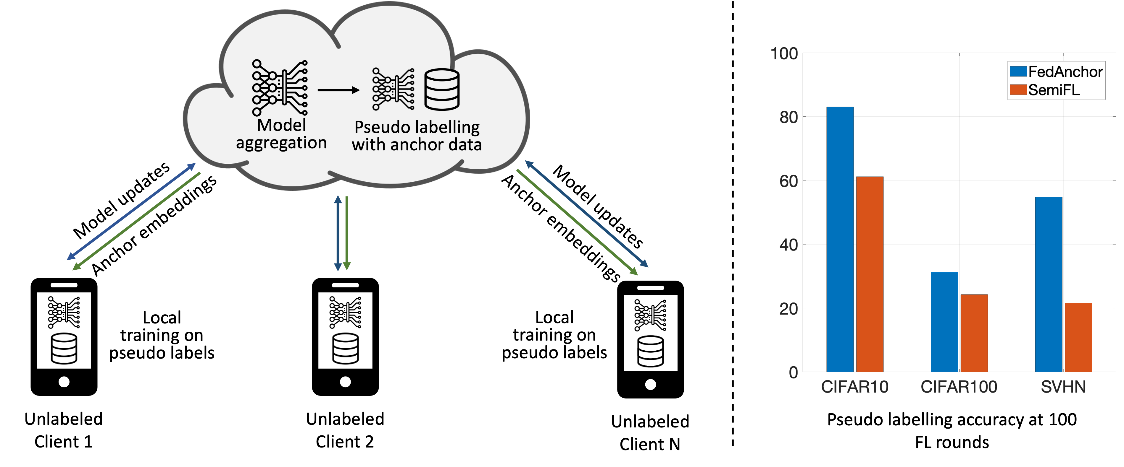
Figure 1: (left) Pipeline of FedAnchor with pseudo labeling and anchor data on the server. (right) Pseudo labeling accuracy with 5000/2500/1000 anchor data on CIFAR10/CIFAR100/SVHN datasets, respectively.

Acquiring large-scale labeled datasets on the user side can be extremely costly, e.g., many unlabeled data samples are generated through interactions with smart devices in daily life, such as pictures or physiological indicators. These volumes of data make it impractical to mandate individual users to annotate the data manually. This task can be excessively time-intensive for users, or they may lack the requisite advanced knowledge or expertise for accurate annotation, particularly when the dataset pertains to a specialized domain such as medical data (Yang et al., 2021) or autonomous driving (Elbir et al., 2020). The complicated process of annotation results in most user data remaining unlabeled, further preventing the conventional FL pipeline from conducting supervised learning. Recent studies of self-supervised learning in FL attempt to leverage unlabeled user data to learn robust representations (Gao et al., 2022a; Rehman et al., 2022, 2023). However, the learned model still requires fine-tuning on labeled data for downstream supervised tasks.

Compared to FL environments, centralized data annotation is more straightforward and precise in data centers. Even in low-resource contexts (e.g., medical data), the task of labeling limited data stored on the server by experts would not demand substantial effort. The integration of semi-supervised learning (SSL) (Chapelle et al., 2009; Yang et al., 2022; Sohn et al., 2020; Berthelot et al., 2019) with FL can potentially leverage limited centralized labeled data to generate pseudo labels for supervised training on unlabeled clients. Existing work (Jeong et al., 2020b; Zhang et al., 2021) attempted to perform SSL by using off-the-shelf methods only, such as FixMatch (Sohn et al., 2020), MixMatch (Berthelot et al., 2019) in FL environments. Although these methods provide certain model convergence guarantees during the FL stage, they cause heavy traffic for data communication due to their per-mini-batch communication protocol. Another recent work, SemiFL (Diao et al., 2022), improves the training procedure by implicitly conducting entropy minimization. This is achieved by constructing hard (one-hot) labels from high-confidence predictions on unlabeled data using existing centralized SSL methods. These are subsequently used as training targets in a standard cross-entropy loss. However, it is argued that using pseudo-labels based on model predictions might lead to a confirmation bias problem or overfitting to easy-to-learn data samples (Nguyen & Yang, 2023). In addition, the existing methods typically establish a pre-defined threshold, generally set relatively high to only keep the high-confident pseudo-labels. This might lead to slow convergence issues, especially at the beginning of training when very limited samples satisfy the threshold.

In this paper, we propose an enhanced federated SSL method, dubbed FedAnchor - a newly designed label contrastive loss based on the cosine similarity metric to train on labeled anchor data on the server. Instead of retaining the high-confidence data solely through model prediction in the conventional SSL studies, FedAnchor for-the-first-time generates the pseudo labels by comparing the similarities between the model representations of unlabeled data and labeled anchor data. This provides better-quality pseudo-labels, as shown in Fig. 1 (right), which alleviates the confirmation bias and reduces the issues of over-fitting to easy-to-learn data samples. Our contributions are summarized as follows: 1) we propose a unique pseudo-labeling method FedAnchor for SSL in FL, which leverages the similarities between feature embeddings of unlabeled data and labeled anchor data; 2) we design a novel label contrastive loss to improve the quality of pseudo labels in FSSL further; 3) we perform extensive experiments on three representative datasets having different amounts of labeled anchor data and show that the proposed methods achieve the state-of-the-art (SOTA) performance with a faster convergence rate.

2 Background

Federated Learning (FL).

FL aims to collaboratively learn a global model while keeping private data on the devices. We consider a $C$ class classification problem defined over a compact space $\mathcal{X}$ and a label space $\mathcal{Y}=[C]$, where $[C]=\{1,...,C\}$. The FL training objective is to minimize: $\min_{w}f(w)=\sum_{k=1}^{N}p_{k}F_{k}(w)=\mathbb{E}_{k}\big{(}F_{k}(w)\big{)}$, where $N$ is the total number of clients in the client pool, $p_{k}>0$ and $\sum p_{k}=1$. In general, the local objectives measure the local empirical risk over possibly differing data distribution $\mathcal{D}_{k}$ of each client, i.e., $F_{k}(w):=\mathbb{E}_{x_{k}\sim\mathcal{D}_{k}}\big{(}f_{k}(w;x_{k})\big{)}$, with $n_{k}$ samples available at each client k. The standard FedAvg (McMahan et al., 2017) method set $p_{k}=\frac{n_{k}}{n}$ where $n=\sum_{k}n_{k}$ is the total number of data points in the systems. $f$ is parameterized over the hypothesis class $w$, which can be seen as the weight of the neural network. $F_{k}$ is the loss function specific to the task.

Semi-Supervised Learning (SSL).

SSL is a problem of learning with partially labeled data, especially when the amount of unlabeled data is much larger than labeled ones (Zhou & Li, 2005; Rasmus et al., 2015). The standard SSL method involves giving pseudo-labels to unlabeled data (Lee, 2013) and using these pseudo-labels as hard labels for supervised training. On the other hand, consistency regularization (Bachman et al., 2014) methods train models by minimizing the distance among stochastic outputs, which can be achieved through different weak or strong augmentations (Cubuk et al., 2020; Thulasidasan et al., 2019; French et al., 2017). Methods such as MixMatch (Berthelot et al., 2019) and FixMatch (Sohn et al., 2020) combine both ideas by imposing a threshold on the model predictions of weak and strong augmented samples, retaining artificial labels only for those with the most significant class probability falling above a pre-defined level.

Federated Semi-Supervised Learning (FSSL).

Considering the difficulties of labeling data in a federated setting, FSSL represents the federated variant of SSL. In this context, we address the more challenging yet realistic scenario where the data stored on the client side is completely unlabeled. Given a dataset $\mathcal{D}=\{\textbf{x}_{i},y_{i}\}^{N}_{i=1}$, which consists of both a labeled set $\mathcal{S}=\{\textbf{x}_{i},y_{i}\}^{S}_{i=1}$, named anchor data in our paper, and an unlabeled set $\mathcal{U}=\{\textbf{x}_{i}\}^{U}_{i=1}$. The unique challenge of FSSL comes from the fact that taking off-the-shelf SSL methods and applying them to FL cannot achieve communication-efficient FL training. For example, techniques such as FixMatch (Sohn et al., 2020) or MixMatch (Berthelot et al., 2019) require each mini-batch to sample from both labeled and unlabeled data samples with a carefully tuned ratio, which is impossible to achieve in real FL settings if the labeled data and unlabeled data are stored in different places. FedMatch (Jeong et al., 2020a) splits model parameters for labeled servers and unlabeled clients separately. FedRGD (Zhang et al., 2021) trains and aggregates the model of the labeled server and unlabeled clients in parallel with the group-side re-weighting scheme while replacing the batch normalization to group normalization.

FedCon (Long et al., 2021) borrows from BYOL (Grill et al., 2020) the idea of using two models and proposes using a consistency loss between two different augmentations to help clients’ networks learn the embedding projection. SemiFL (Diao et al., 2022) takes the centralized SSL method MixMatch (Berthelot et al., 2019) with mixup (Thulasidasan et al., 2019) augmentation method together with an alternate training scheme (Gao et al., 2022b; Dimitriadis et al., 2020) to achieve the current SOTA performance. However, the simple combination of existing centralized SSL methods with different augmentation approaches in SemiFL insufficiently improves the quality of pseudo-labeling. Both FedCon and SemiFL serve as baselines in our paper.

Latent Representation.

The great success neural networks have achieved since their introduction is to be adjudged to their capability of learning latent representations of the input data that can eventually be used to learn the task they have been designed for. The set containing this latent information is often referred to as latent space, which can also be the subject of topological investigation (Zaheer et al., 2017; Hensel et al., 2021). Many theoretical studies have highlighted the importance of such representations as they are explicitly identified in many settings, e.g., the intermediate layers of a ResNet architecture (He et al., 2016), the word embedding space of a language model, or the bottleneck of an Autoencoder (Moor et al., 2020). More recently, the research community focused on investigating the quality of the latent space as well-performing networks have shown similar learned representations (Li et al., 2015; Morcos et al., 2018; Kornblith et al., 2019; Tsitsulin et al., 2019; Vulić et al., 2020). Despite these speculations being found to be more empirical than theoretical, the interest in leveraging latent representation to enhance or facilitate training methods, especially those not relying on labeled data, has increased.

The most audacious attempt to leverage the structure of different latent spaces is presented in (Morcos et al., 2018). The authors of the latter leveraged interesting observations regarding the structure of different latent spaces learned by diverse training procedures to achieve zero-shot model stitching. While we refer the reader to their paper for the details, we want to highlight one observation and one method that makes their work relevant to ours. First, they showed that differently-learned latent spaces are the same up to an approximately isometric transformation. Second, they used the latter observation to construct a method based on “anchor” samples and the “cosine similarity” metric.

3 Motivation

Most current SSL methods, as mentioned in Section 2, are based on augmentation methods and pseudo-labels obtained from the prediction of the training model. This method not only gives confirmation bias and overfitting to easy-to-learn data samples (Nguyen & Yang, 2023), but it also makes the number of training samples qualified for training very small, i.e., an unlabeled sample will only be considered for pseudo-labeling when the probability of a given class is above a pre-defined and difficult-to-tune confidence threshold (often set as $0.95$ for high confidence).

We now present preliminary investigations on the current SOTA method, SemiFL, to showcase these shortcomings. We run these investigations on the CIFAR10 dataset (Krizhevsky, 2012) under the FL settings when it is partitioned non-IID ($\alpha=0.1$) over $100$ clients, with $10$ clients selected for training during every communication round. More details of the experimental protocols can be found in Section 5.1. In this section, we demonstrate two different setups with different anchor sizes, $250$ and $500$.

Figure 2 demonstrates that the average number of samples per client satisfying the threshold condition is very low. For the CIFAR10 dataset, every client has $500$ data samples after the partition, but as we can see from the figure, the maximum number of samples satisfying the condition is below $60$, and on average, it is below $25$ for anchor size of $500$ and below $20$ for the anchor size of $250$. Therefore, the training procedure cannot efficiently take advantage of the information available, resulting in a slower convergence rate. This training method incurs unnecessary communication costs, which can be more energy-consuming, as shown in previous work (Qiu et al., 2023).

Our other baseline, FedCon (Long et al., 2021) shows another shortcoming: choosing the best augmentation for the task is crucial for its consistency loss to work. Moreover, in addition to tuning standard FL-related hyperparameters, FedCon requires careful tuning of several local and global optimization steps. The flexibility and robustness of FedAnchor overcome the shortcomings of previous proposals that rely too much on difficult-to-tune hyperparameters and specific augmentations.

The quality of the pseudo-labels generated by the FedAnchor allows for overcoming previous works’ shortcomings while using the same amount of samples on the server. Thus, a potential application in the wild to a more extensive federated population will require the construction of a smaller dataset at the server to serve as anchor compared to the baselines. The model achieves a better convergence rate and performance using our more efficient training procedure using the same number of anchor samples.

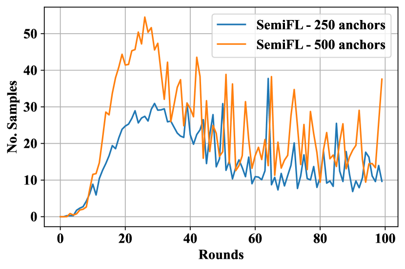
Figure 2: The average number of qualified data samples trained by selected clients in each round, for CIFAR10 Non-IID ($\alpha=0.1$) partition with $250$/$500$ anchor data on the server, using method SemiFL. The plot shows that the average number of data samples trained by clients is very small, given each client has a total of $500$ training data samples.

4 Methodology: FedAnchor

In this section, we present our method FedAnchor (Fig. 1) in detail. FedAnchor aims to fully utilize the information embedded in the anchor dataset stored on the server to provide better pseudo-labels for unlabeled private client’s data to be trained on supervised tasks. We propose a novel label contrastive loss combined with cosine similarity metrics to extract the anchor information in the latent space. The section is organized as below: we detail the new label contrastive loss in Section 4.1; we then explain in Section 4.2 how to obtain the pseudo label in our methods; then it is followed by the algorithm of local training on the client side in Section 4.3 and the server training using anchor data in Section 4.4. The pseudo-code of the FedAnchor is summarized in Algorithm 1.

We define the $x^{m}$ to be the unlabeled data samples on client $m$; $(x^{anchor},y^{anchor})$ be the labeled anchor data; $z^{m}$ be the output of the anchor head (latent space) for the unlabeled client data, and $z^{anchor}$ be the output of the anchor head (latent space) for the anchor data. Hence, the symbol $z$ always represents any given data sample’s latent representation. Also, $\hat{y}$ denotes the pseudo-label for unlabeled data.

4.1 Label contrastive loss

One of the main novelties of our method lies in introducing a new label contrastive loss that acts on the latent space. As mentioned in the background section (Section 2), the latent space retains important representations that can be identified and utilized in many settings. In our case, the latent space can be the output of any pre-defined layer in the neural network. However, since our method modifies the underlying geometry of the chosen output layer, we suggest picking a later layer to let the earlier ones maintain their feature extraction capabilities. A visualization can be found in Appendix D.

FedAnchor uses a double-head structure for the model, with one head (classification head) consisting of the original classification layers and the other (anchor head) consisting of a projection layer to the latent space to reduce the previous embedding dimension. The anchor head is crucially designed to work with the new label contrastive loss that we propose below. Despite its complexity, this structure is model agnostic and can be implemented in all the deep learning model architectures used for a classification task.

The label contrastive loss aims to map the $z^{anchor}$ of the same label to the same local region in the latent space while forcing data with different labels to be far from each other. We let $s_{i,j}$ be any similarity function between data sample $x_{i}$ and $x_{j}$ in the latent space ($z_{i}$,$z_{j}$). Cosine similarity is used in our case: $s_{z_{i},z_{j}}=\frac{z_{i}^{T}z_{j}}{\lVert z_{i}\rVert\lVert z_{j}\rVert}$.

Then, we propose our new label contrastive loss as in eq. 1 and 2. The label contrastive loss is defined on a batch of anchor data samples. Given a batch of anchor data, we calculate the $l(c)$ for each label class, then sum up all label classes to obtain the final value of the label contrastive loss.

$$l(c)=-\log \frac{\sum_{y(i),y(j)=c}\exp(s_{z_{i},z_{j}}/\tau)}{\sum_{y(i)\not=y(j)}\exp(s_{z_{i},z_{j}}/\tau)}$$ (1)

$$\mathcal{L}_{c} =\frac{1}{C}\sum_{c=1}^{C}l(c)$$ (2)

where $\tau$ is the tunable temperature hyper-parameter. During the training, the label conservative loss tends to maximize the similarities between samples with the same labels while minimizing the similarities between samples with different labels. Crucially, the proposed loss will correct the projections of the data samples by modifying the underlying geometry of the projector part of the model.

4.2 Pseudo-labeling using anchor head

We present our pseudo-labeling method by describing a single communication round, the unit of iteration in FL, step-by-step. At the communication round $t$, the server selects a subset of clients to participate with participation ratio $r$ in the current federated round. The server will then broadcast the model parameters ($w_{t}$) and the latent anchor representations ($\{z^{anchor}_{i}\}_{i=1}^{S}$) to the selected clients. The anchor latent representations are the output of the anchor head, which generates the hard pseudo-label during training.

After receiving the current model weights and anchor latent representations, each client $m$ computes the latent representation of each local data ($\{z^{m}_{i}\}_{i}$). Then, it compares $z^{m}_{i}$ to each anchor latent representation ($\{z^{anchor}_{i}\}_{i=1}^{S}$) to obtain the pseudo-label leveraging the cosine similarity between $z^{m}_{i}$ and each anchor latent representation. The scores obtained from this comparison are averaged by label, i.e., cosine similarities relative to anchor latent representation from anchor samples with the same label are averaged. The pseudo-label is the label that provides the maximum score.

Let $Z^{anchor}_{c}=\{z^{anchor}_{i}\in S~{}|\ y^{anchor}_{i}=c\}$ be the set of anchor latent representation with label $c$. Then, the average cosine similarities between $z^{m}_{i}$ and each $Z_{c}$ can be computed. Let $s^{avg}$ be the average similarities of a data input compared with anchor data. $s^{avg}_{c}(z^{m}_{i})$ is the average cosine similarities between unlabeled data latent representation $z^{m}_{i}$ compared with each anchor data with label class $c$. The value of $s^{avg}_{c}(z^{m}_{i})$ can be calculated as:

$$s^{avg}_{c}(z^{m}_{i})=\frac{1}{|Z^{anchor}_{c}|}\sum_{z_{k}\in Z^{anchor}_{c}}s(z^{m}_{i},z_{k}),$$ (3)

Subsequently, to obtain the pseudo-label $\hat{y}^{m}_{i}$ for each local data, we need to find the label class that produces the maximum $s^{avg}_{c}(z^{m}_{i})$:

$$\hat{y}^{m}_{i}=argmax_{c\in[C]}\big{(}s^{avg}_{c}(z^{m}_{i})\big{)}.$$ (4)

It is worth noting that cosine similarity is well-known for being low complexity and highly optimizable (Novotnỳ, 2018). Such operations are independent and completely parallelizable. As a result, it is feasible to scale up to cases where clients and server contains a large amount of data.

4.3 Local training

After obtaining the pseudo-labels ($\hat{y}^{m}$) for the local data, each client will locally perform supervised training using the pseudo-labels as hard labels. As mentioned in Section 2, semi-supervised training methods often leverage different data augmentation procedures – weak or strong augmentation methods, such as RandAugment (Cubuk et al., 2020). These perform differently depending on the dataset, model, and task. We used the mixup (Thulasidasan et al., 2019) method to obtain a fair comparison with SemiFL. The mixup method trains a neural network on convex combinations of pairs of examples and their labels with coefficients generated by the beta distribution. This can potentially improve the robustness of the model and utilize the limited labeled data. It is important to notice that FedAnchor is completely agnostic on the augmentation used, as opposed to FedCon, whose consistency loss’s performance strongly depends on the specific augmentation. The detailed implementation of mixup methods can be found in Appendix B.

4.4 Server training

We aim to use the labeled anchor data on the server as training data for supervised and label contrastive loss to leverage the information they carry fully. Training at the server on the labeled data is not novel (Gao et al., 2022b; Dimitriadis et al., 2020) as SemiFL (Diao et al., 2022) performs this dubbing alternate training procedure. However, by comparison, FedAnchor trains on the anchor data at the server in two epochs: one for the supervised classification loss and one for the label contrastive loss to further improve the pseudo-label accuracies during every round. Let $\mathcal{L}_{s}$ be the supervised training loss, such as the standard cross-entropy loss for the classification task, and $\mathcal{L}_{c}$ be the label contrastive loss described in Section 4.1. Therefore, the server will train for one epoch on the classification head by minimizing the loss $\mathcal{L}_{s}$ and for one epoch on the anchor head by minimizing the loss $\mathcal{L}_{c}$.

Table 1: Comparison of FedAnchor with the state-of-the-art methods and fully supervised baseline on model ResNet-18. FedAnchor (mix) represents the experiments conducted using FedAnchor, but the supervised training on the server with anchor data is replaced with the mixup method explained in Section 4.5. Supervised models are trained with standard FL procedure with alternative training on the server, initialized from a pre-trained model on anchor data.

Datasets		CIFAR10			CIFAR100		SVHN
Number of anchor data		250	500	5000	2500	10000	250	1000
IID ($Dir=1000$)	Supervised	89.45 ± 0.47	89.73 ± 0.09	89.07 ± 0.22	61.84 ± 0.17	63.33 ± 0.21	95.38 ± 0.03	94.87 ± 0.53
	FedCon	34.94 ± 0.43	50.81 ± 3.21	74.95 ± 1.26	32.84 ± 0.40	50.05 ± 0.34	54.83 ± 2.77	83.92 ± 1.03
	FedAvg+FixMatch	33.98 ± 1.77	49.18 ± 2.33	75.42 ± 0.73	32.31 ± 0.83	49.15 ± 0.57	43.61 ± 0.64	81.65 ± 1.83
	SemiFL	77.82 ± 0.49	81.19 ± 0.35	75.46 ± 0.19	48.20 ± 0.63	63.68 ± 0.16	91.55 ± 0.77	90.11 ± 1.17
	FedAnchor	80.36 ± 0.18	85.94 ± 0.11	83.52 ± 0.41	50.79 ± 0.27	62.02 ± 0.24	91.74 ± 0.41	92.77 ± 0.11
	FedAnchor (mix)	82.82 ± 0.21	85.87 ± 0.25	84.43 ± 0.36	51.34 ± 0.07	63.99 ± 0.39	87.46 ± 0.63	92.71 ± 0.54
Non-IID ($Dir=0.1$)	Supervised	75.42 ± 5.64	77.96 ± 2.55	77.99 ± 1.24	50.87 ± 1.64	60.47 ± 0.52	87.48 ± 4.78	91.29 ± 0.33
	FedCon	38.46 ± 0.42	51.57 ± 1.34	76.38 ± 1.36	32.00 ± 0.46	48.61 ± 0.56	50.86 ± 1.50	83.40 ± 1.89
	FedAvg+FixMatch	39.10 ± 0.17	49.92 ± 2.49	73.17 ± 1.33	34.43 ± 0.87	49.53 ± 0.56	47.09 ± 1.31	76.83 ± 3.26
	SemiFL	58.82 ± 0.72	68.96 ± 0.98	72.12 ± 0.35	42.41 ± 0.47	59.72 ± 0.31	68.97 ± 13.24	87.21 ± 1.66
	FedAnchor	60.19 ± 0.32	72.75 ± 0.63	81.37 ± 0.31	43.50 ± 0.13	59.96 ± 0.40	77.42 ± 0.55	90.20 ± 0.56
	FedAnchor (mix)	62.94 ± 0.52	73.02 ± 0.31	83.59 ± 0.46	46.39 ± 0.36	61.01 ± 0.06	60.30 ± 5.34	87.28 ± 0.08

4.5 Possible Additions

Since the assumptions we made to design FedAnchor are simple and general, numerous potential extensions can be added to the above-described pipeline. One addition can be made to the supervised training on the server. Instead of only using strong augmentation, we can implement the same idea of mixup augmentation with a loss function.

Additionally, at the pseudo-labeling stage (Section 4.2), instead of feeding the raw and original unlabeled training data, we can borrow the idea of consistency regularization and pseudo-label ensembles techniques (Bachman et al., 2014; Sajjadi et al., 2016) to weakly augment the unlabeled training data ($\alpha(x^{m}_{i})$) for a few times and then take the ensembles to generate more robust pseudo-labels.

5 Experiments

Table 2: Comparison of FedAnchor with the state-of-the-art methods and fully supervised baseline on model Wide-Resnet28x2.

Datasets		CIFAR10			CIFAR100		SVHN
Number of anchor data		250	500	5000	2500	10000	250	1000
IID ($Dir=1000$)	Supervised	83.91 ± 1.82	84.48 ± 0.48	80.81 ± 1.05	61.15 ± 0.69	63.38 ± 0.19	92.86 ± 1.15	91.41 ± 0.70
	FedAvg+FixMatch	46.59 ± 1.56	54.50 ± 1.60	77.57 ± 1.17	32.71 ± 0.19	50.99 ± 0.28	60.87 ± 1.49	83.07 ± 2.16
	FedCon	39.43 ± 1.08	53.25 ± 1.28	75.82 ± 1.54	30.82 ± 0.19	49.04 ± 0.86	57.08 ± 0.73	81.57 ± 1.49
	SemiFL	71.83 ± 1.10	67.29 ± 2.98	77.04 ± 0.50	38.86 ± 0.33	52.50 ± 0.23	90.36 ± 0.43	89.39 ± 0.39
	FedAnchor	79.52 ± 0.07	81.73 ± 0.43	80.72 ± 0.41	44.98 ± 0.30	53.56 ± 0.45	90.85 ± 0.27	91.86 ± 0.09
	FedAnchor (mix)	80.06 ± 0.62	81.16 ± 0.43	83.76 ± 0.23	46.79 ± 0.32	56.40 ± 0.11	90.18 ± 0.36	91.88 ± 0.18
Non-IID ($Dir=0.1$)	Supervised	78.54 ± 0.52	74.85 ± 0.82	79.50 ± 0.46	55.87 ± 0.63	59.01 ± 0.30	87.34 ± 0.88	87.48 ± 1.49
	FedAvg+FixMatch	41.09 ± 1.42	53.29 ± 1.20	77.32 ± 0.76	32.01 ± 0.25	50.75 ± 0.47	52.96 ± 0.75	83.39 ± 0.67
	FedCon	41.11 ± 0.31	52.25 ± 1.90	75.20 ± 0.42	30.27 ± 0.98	49.16 ± 0.80	57.98 ± 1.49	76.78 ± 2.57
	SemiFL	49.97 ± 0.64	56.99 ± 1.85	76.86 ± 0.82	38.26 ± 0.32	52.08 ± 0.31	61.87 ± 1.05	85.97 ± 0.52
	FedAnchor	52.93 ± 0.95	63.38 ± 0.64	80.33 ± 0.19	40.89 ± 0.23	52.85 ± 0.20	63.81 ± 0.41	86.39 ± 0.33
	FedAnchor (mix)	55.26 ± 0.92	64.96 ± 0.27	82.70 ± 0.70	42.25 ± 0.38	55.26 ± 0.37	48.56 ± 0.30	86.09 ± 0.06

Table 3: (upper) Comparison of FedAnchor with baselines on model Wide-ResNet28x2 under different augmentation setups. (lower) Ablation study on model ResNet-18. FedAnchor(w/o contr loss) represents using embeddings similarities for pseudo-labeling without contrastive loss. Both are conducted on Non-IID ($Dir=0.1$) FL setting.

Datasets		CIFAR10	SVHN
Anchor Size		500	1000
Wide ResNet28x2	FedAvg+FixMatch	53.29 ± 1.20	83.39 ± 0.67
	SemiFL	56.99 ± 1.85	85.97 ± 0.52
	SemiFL+no mixup	62.93 ± 0.85	84.93 ± 0.99
	FedAnchor(client mixup)	63.38 ± 0.64	86.39 ± 0.33
	FedAnchor(no mixup)	63.15 ± 0.15	87.78 ± 0.31
	FedAnchor(client & server mixup )	64.96 ± 0.27	86.96 ± 0.08
	FedAnchor(server mixup)	66.07 ± 0.50	86.09 ± 0.06
ResNet-18	SemiFL	68.96 ± 0.98	87.21 ± 1.66
	FedAnchor(w/o contr loss)	70.90 ± 0.03	88.13 ± 0.35
	FedAnchor	72.75 ± 0.63	90.20 ± 0.56

5.1 Experimental setup

The information regarding the exact implementation and packages can be found in the Appendix G.

Federated datasets. We conduct experiments on CIFAR-10/100 (Krizhevsky, 2012) and SVHN (Netzer et al., 2011) datasets. The training set is randomly split into labeled anchor data and unlabeled clients’ data for all datasets so that the testing set remains the same for all anchor settings. To make a fair comparison, we set the number of labeled anchor data samples for CIFAR-10/100 and SVHN datasets to be {$250$, $500$, $5000$}, {$2500$, $10000$} and {$250$, $1000$} respectively, according to popular SSL setups (Sohn et al., 2020; Berthelot et al., 2019). To simulate a realistic cross-device FL environment using the rest of the data, we generate IID/non-IID versions of datasets based on actual class labels using Latent Dirichlet Allocation (LDA) with coefficient $Dir$ (Qiu et al., 2022; Reddi et al., 2021), where a lower value indicates greater heterogeneity. As a result, the datasets are randomly partitioned into $100$ shards with $Dir=\{1000,0.1\}$ for IID and non-IID settings, respectively.

Training hyper-parameters. Following some previous literature, such as MixMatch (Berthelot et al., 2019), FixMatch (Sohn et al., 2020) or SemiFL (Diao et al., 2022), we implemented Wide ResNet28x2 (Zagoruyko & Komodakis, 2016) as the backbone model for all datasets. In addition, we also implemented the most standard version of ResNet-18 (He et al., 2016) to demonstrate the effectiveness of our method on the standard architecture. The anchor head is set to be a linear layer with $128$ dimensions. During each FL round, $10$ clients are randomly selected to participate in the training for $5$ local epochs. The FL training lasts for $500$ rounds. Our implementation of FedCon (Long et al., 2021) is based on the original GitHub repository (Appendix G), from which we extracted both the client and server training pipeline and put them in our codebase. In the original FedCon paper, only the simple model architectures are tested. We replaced the original backbone with ours to perform a fair comparison. More details regarding hyperparameters and baseline implementations can be found in Appendix C.

5.2 Results

Table 1 and 2 show the performance of FedAnchor along with the baselines Fed+FixMatch, SemiFL (Diao et al., 2022), FedCon (Long et al., 2021). First, the FedAnchor outperforms these baselines in all settings and datasets. Specifically, training with a minimal number of anchor data samples (e.g., 25 samples per label) can yield satisfactory performance in IID FL settings. Increasing the anchor data can drastically boost performance in the more challenging but realistic non-IID settings. Indeed, this condition is not difficult to meet as numerous labeled data, suitable to be used as anchors, are stored in centralized data centers. More detailed results can be found in Fig. 3 (a) & (b), which demonstrates the superiority of FedAnchor. Additional graphs can be found in Appendix E.

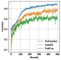
(a) Anchor 250

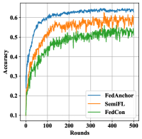
(b) Anchor 500

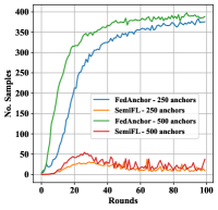
(c) No. of samples

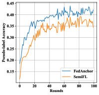
(d) Pseudo-label Acc

Figure 3: Results on CIFAR10 Non-IID with different anchor sizes. (a) and (b) show the testing accuracy with different methods on the two anchor setups. (c) shows the average number of samples selected for training on each client. (d) shows the pseudo-label accuracy of the 500 anchor case (to avoid too many lines in one graph, we show the 500 anchors case, but the general trend is the same for other cases), which shows that pseudo-labels generated by FedAnchor are consistently above the baseline method. (c) and (d) are smoothed every $5$ rounds.

Compared to the baseline SemiFL and FedCon, our methods provide more stable performance, lower standard deviation, and a much faster convergence rate. Indeed, this proves beneficial when deploying this method in real-world applications or industrial contexts. The experimental results for SemiFL under SVHN non-IID with 250 anchor data are extremely volatile and slow to converge. It largely depends on the random process, yielding much unstable accuracy. FedCon consistently underperforms in comparison to SemiFL.

In addition, using the mixup method in the server training process obtains slightly enhanced performance in most cases. This improvement is primarily attributable to the ample use of data, which is advantageous for training a more robust model (Berthelot et al., 2019). Utilizing mixup method locally on the client-side training can also boost the performance. We can observe across all datasets that alternative training with more anchor data samples on the server can make the difference between IID and non-IID smaller because the anchor data can be seen as a “shared IID data” that can reduce heterogeneity across clients.

Figure 4 shows that FedAnchor can reduce the confirmation bias compared with the baseline. The figure demonstrates that SemiFL, which uses model prediction as the pseudo-labels, degenerates after $300$ rounds, even with the IID partitions. It is clear from the figure that the accuracy stops increasing, which indicates that the model is overfitting to the easier data samples and generating poorer pseudo labels, resulting in lower testing accuracy.

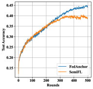
(a) Test Accuracy

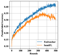
(b) Pseudo-label Accuracy

Figure 4: Plots on CIFAR100 (IID, 2500 anchors) experiment. (a) testing accuracy. (b) pseudo-label accuracy. FedAnchor can reduce the confirmation bias compared to SemiFL.

We also conduct ablation studies on the naive implementation of FixMatch (Sohn et al., 2020), the centralized SOTA method, under the FL setups, as shown in Table 1 & 2, to show the effect of the label contrastive loss and the proposed pseudo-labeling. As mentioned in Section 2, the original centralized setting of FixMatch requires sampling both labeled and unlabeled data per mini-batch. Therefore, implementing FedAvg+FixMatch combines FixMatch locally on the client side and alternative training using anchor data on the server side. We can see that the simple combination of FedAvg and FixMatch fails to produce excellent performance.

In addition, we experiment with different augmentation arrangements as shown in Table 3, which demonstrates that utilizing the mixup method on the client side, as SemiFL did, might not always lead to the best performance. However, FedAnchor still outperforms in all augmentation cases.

5.3 Pseudo labeling quality

The quality of pseudo-labels can largely determine the convergence rate of the training and its resulting performance. As unlabeled client training data is trained with generated hard pseudo-labels, with higher pseudo-label accuracy, the model can extract more useful information from the unlabeled client data, converging to better performance with a faster convergence rate.

As previously shown in Section 3, the average number of samples trained by each client for the method SemiFL can be less than $10\%$ of the total samples stored on the client side. We compare the average number of samples trained by clients for FedAnchor with SemiFL in Fig. 3(c). As demonstrated in the figure, the average number of samples trained by each client grows with the training round, which is as expected since the model is trained to improve gradually. The average number is growing to almost $400$ for FedAnchor compared with consistently below $100$ for SemiFL. This is presumably attributed to the higher quality of the pseudo-labels generated by FedAnchor.

To substantiate this claim, we compute the pseudo-label accuracy by comparing the pseudo-labels generated by different methods with the true labels, as shown in Fig. 3 (d) & 4(b). Clearly, FedAnchor can produce higher pseudo-label accuracy with a big margin compared to the baseline method. More results can be found in Appendix F.

5.4 Ablation studies

We conduct an ablation study by refining the pseudo-labeling method in SemiFL using the similarities between feature embeddings of unlabeled data and labeled anchor data, notably excluding the use of contrastive loss in the training process. One can see from Table 3 (lower part) that adopting our new pseudo-labeling approach with anchor data slightly boosts the performance. However, including contrastive loss is imperative to achieve a significantly higher accuracy.

5.5 Communication Overhead

As we know from (Qiu et al., 2023), communication cost is one of a big concern in FL. Table 4 shows the communication overhead of FedAnchor compared to standard supervised FL training. The overhead is only for downstream communication when extra anchor embeddings must be sent from the central server to the selected clients. The overhead is calculated as the percentage of transmitted parameters that compose the anchors’ embeddings over the number of the model’s parameters transmitted by FedAvg: $Overhead=\frac{100}{\dim(\bar{w})}\sum_{i=1}^{S}\dim(z_{i}^{anchor})$, where $\bar{w}$ is the model transmitted by FedAvg. The upstream communication is the same as FedAvg. Thus, the extra communication overhead of FedAnchor is negligible compared to the one during standard FL training.

Table 4: Downstream communication overhead of FedAnchor compared with supervised FL training.

Datasets	Anchor Size	Overhead
CIFAR10	250 / 500 / 5000	0.29$\%$ / 0.57$\%$ / 5.73$\%$
CIFAR100	2500 / 10000	2.85$\%$ / 11.41$\%$
SVHN	250 / 1000	0.29$\%$ / 1.15$\%$

6 Conclusion

In this paper, we propose FedAnchor, which is a FSSL method enhanced by a newly designed label contrastive loss based on the cosine similarity to train on labeled anchor data on the server. Instead of retaining the high-confidence data solely through model predictions as in the conventional SSL studies, FedAnchor generates the pseudo labels by comparing the similarities between the model representations of unlabeled data and labeled anchor data. This provides better quality pseudo-labels, alleviates the confirmation bias, and reduces the issues of over-fitting to easy-to-learn data samples. We perform extensive experiments on three different datasets with different sizes of labeled anchor data on the server and show that the proposed methods achieve state-of-the-art performance with a faster convergence rate. As for future direction, we are experimenting with a fixed threshold during the pseudo-labeling using the anchor data stage. More advanced adaptive and dynamic thresholding techniques can be implemented to improve the performance and convergence rate further.

Impact Statement

This paper presents work whose goal is to advance the field of Decentralized Machine Learning. There are many potential societal consequences of our work, none of which we feel must be specifically highlighted here.

Appendix A Algorithm pseudo code

Algorithm 1 FedAnchor: Let $N$ be the total number of clients, with total $n$ data samples; $(x^{m})$ be the unlabeled data in client $m$; $(x^{anchor},y^{anchor})$ be the labeled anchor data in the server; $z^{m}$ be the output of the latent space for the unlabeled client data, and $z^{anchor}$ be the output of the latent space for the anchor data; we let $\hat{y}$ be the pseudo-label for unlabeled data; $E$ be the number of local epochs; $r$ be the participation ratio of clients in each round; $w_{t}$ be the aggregated weights at round $t$; $C$ be the total number of labels; $Z^{anchor}$ be the set of anchor latent representation; $\eta_{clt}$ and $\eta_{ser}$ be the client and server learning rate respectively. ClientTraining be the training procedure on the client using the local dataset, and ServerTraining be the training procedure on the server using the anchor dataset.

1:  Procedure Server executes

2:  Initialize the model weight $w_{0}$

3:  for t = 1,…,T do

4:     $M_{t}\leftarrow$ random select $(rN)$ number of clients

5:     compute $Z^{anchor}$

6:     for  each $m\in M_{t}$ do

7:        $\hat{y}^{m}\leftarrow$ Pseudo Label($x_{m},Z^{anchor}$)

8:        $w_{t+1}^{m}\leftarrow$ ClientTraining$(w_{t},x_{m},\hat{y}^{m})$

9:     end for

10:     $w_{t+1}\leftarrow\sum_{m\in M_{t}}\frac{n_{m}}{\sum n_{m}}w_{t+1}^{m}$

11:     $w_{t+1}\leftarrow$ ServerTraining($w_{t+1},x^{anchor},y^{anchor}$)

12:  end for

13:  Procedure Pseudo Label($x_{m},Z^{anchor}$)

14:  for i = 1,…,$|x_{m}|$ do

15:     create label-specific anchor projected set like below:

16:     $Z^{anchor}_{c}=\{z^{anchor}_{i},y^{anchor}_{i}=c\},\forall c\in[C]$

17:     $s^{avg}_{c}(z^{m}_{i})=\frac{\sum_{z_{k}\in Z^{anchor}_{c}}s(z^{m}_{i},z_{k})}{|Z^{anchor}_{c}|}$ (eq. 3)

18:     $\hat{y}^{m}_{i}=argmax_{c\in[C]}\big{(}s^{avg}_{c}(z^{m}_{i})\big{)}$ (eq. 4)

19:  end for

Appendix B Mixup training methods

In this section, we explain the mixup method implemented in detail.

Each selected client needs to construct a high-confidence dataset $\mathcal{D}^{fix}_{m}$, which is called the fix dataset inspired by FixMatch (Sohn et al., 2020) and SemiFL (Diao et al., 2022). The fix dataset is defined to be the set of data samples with the similarity scores above the preset threshold $t$:

$$\mathcal{D}^{fix}_{m}=\{(x^{m}_{i},\hat{y}^{m}_{i})\ \ \verb!s.t.!\max\big{(}s^{avg}_{c}(z^{m}_{i})\big{)}>t\}.$$ (5)

The current local training will be stopped if the client has an empty fix dataset. Otherwise, we then will sample with replacement to construct a mix dataset inspired by MixMatch (Berthelot et al., 2019) as below:

$$\mathcal{D}^{mix}_{m}=\verb!Sample!|\mathcal{D}^{fix}_{m}|\verb! with replacement from !\{(x^{m}_{i},\hat{y}^{m}_{i})\}$$ (6)

where $|\mathcal{D}^{fix}_{m}|$ represents the size of the fix dataset, and in this case $|\mathcal{D}^{fix}_{m}|=|\mathcal{D}^{mix}_{m}|.$

During local training with a nonempty fix dataset, the loss function $\mathcal{L}$ consists of two parts: $\mathcal{L}_{fix}$ and $\mathcal{L}_{mix}$. $\mathcal{L}_{fix}$ is calculated as in standard supervised training with mini-batch sampled from the fix dataset, but attaching strong augmentation $A(\cdot)$ on each data input:

$$\mathcal{L}_{fix}=l\big{(}f\big{(}A(x^{fix}_{b}),\hat{y}^{fix}_{b}\big{)}\big{)}.$$ (7)

where $l$ is the loss function, such as cross-entropy loss for classification tasks.

In addition, the mix loss $\mathcal{L}_{mix}$ is computed following the Mixup method. Client $m$ constructs a mixup data sample from one fix data $x^{fix}$ and one mix dataset $x^{mix}$ by:

$$\lambda_{mix}\sim Beta(a,a),\ x_{mix}=\lambda_{mix}x^{fix}+(1-\lambda_{mix})x^{mix},$$ (8)

where $Beta(a,a)$ represents the beta distribution and $a$ is a mixup hyperparameter, and the mix loss is calculated as:

$$\mathcal{L}_{mix}=\lambda_{mix}\cdot l\big{(}f\big{(}\alpha(x_{mix},\hat{y}^{fix})\big{)}\big{)}+(1-\lambda_{mix})\cdot l\big{(}f\big{(}\alpha(x_{mix},\hat{y}^{mix})\big{)}\big{)},$$ (9)

where $\alpha(\cdot)$ represents weak augmentation of data samples. A single local epoch of a client $m$ corresponds to applying as many local SGD steps on the combined loss as the number of batches it has in $\mathcal{D}^{mix}_{m}$:

$$\mathcal{L}_{combine}=\mathcal{L}_{fix}+b\mathcal{L}_{mix},$$ (10)

where $b$ can be a linear combination coefficient and set to be $1$ as default.

Finally, after operating for $E$ local epochs, client $m$ returns the updated model parameters to the central server to finish the local training.

Appendix C Training Hyper-parameters

Before FL, the model is pre-trained on anchor data on the server for $5$ epochs with SGD to speed up the training process with a learning rate of $0.05$. We use a learning rate of $0.03$, a weight decay of $5e-4$, and an SGD momentum of $0.9$ for both local training on the client side and anchor training on the server side. As indicated in the paper, the threshold is set to $0.6$ for our method and $0.95$ for the SemiFL baseline. We conduct three random experiments for all the datasets with different seeds, and the performance is reported on the centralized test set. The hyperparameter for the beta distribution of mixup (eq.8) is $a=0.75$, and the linear coefficient combining fix loss and mix loss $b$ (eq. 10) is $1$ for all experiments. We implement RandAugment (Cubuk et al., 2020) as a robust augmentation method.

We have also included the federated supervised training as one of the baselines. The supervised implementation follows the standard experimental protocol as per previous papers (Reddi et al., 2021; Qiu et al., 2022; Horvath et al., 2021), where no strong augmentation methods are implemented.

Appendix D Latent space visualization

Figure 5 provides a visualization of the latent space of the model at different stages of the FL using FedAnchor. The visualization demonstrates that FedAnchor can successfully separate the classes in the latent space through the training process.

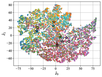
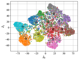
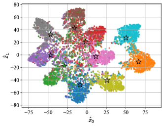
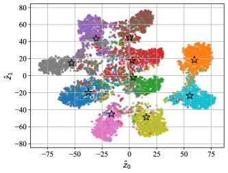
Figure 5: Visualization of the latent space of the model at different stages of the FL using FedAnchor. A t-SNE dimensionality reduction has been performed to improve readability. CIFAR-10 with Wide ResNet backbone is represented here. Different colors refer to different labels. Each data point is representative of a data sample in the (centralized) test set of CIFAR-10. The stars (★) represent the centroids for each label. The rounds represented in (a), (b), (c), and (d) are respectively $1$ (after one aggregation), $100$, $200$, and $500$ (final global model).

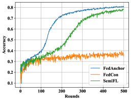
(a) IID ($Dir=1000$) - 250 anchors

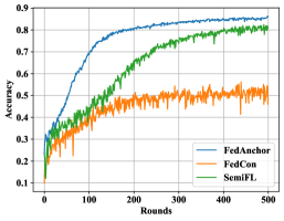
(b) IID ($Dir=1000$) - 500 anchors

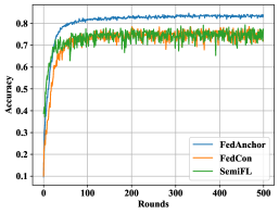
(c) IID ($Dir=1000$) - 5000 anchors

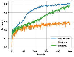
(d) non-IID ($Dir=0.1$) - 250 anchors

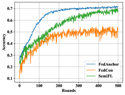
(e) non-IID ($Dir=0.1$) - 500 anchors

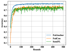
(f) non-IID ($Dir=0.1$) - 5000 anchors

Figure 6: Performance on CIFAR10 test set on ResNet-18 with both IID and non-IID cases across different numbers of anchor data setups, compared with the baseline.

Appendix E More Experimental Results

In this section, we provide some additional plots testing on ResNet-18 as shown in Figure 6 (CIFAR10), 7 (CIFAR100) and 8 (SVHN). All plots indicate that the FedAnchor outperforms the baseline significantly. FedCon consistently underperforms both FedAnchor and SemiFL. SemiFL usually has very slow convergence at the beginning of the training, as we expect, as the prediction of the model is bad at the beginning, which leads to a very limited number of training samples satisfying the threshold. We can also see that SemiFL normally generates a very unstable training curve, especially for the SVHN 250 anchors case, which also indicates the less effectiveness of using model prediction for pseudo-labeling.

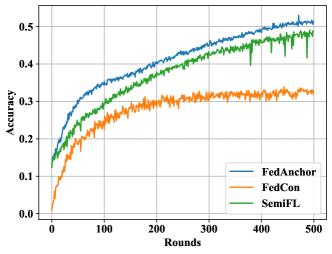
(a) IID ($Dir=1000$) - 2500 anchors

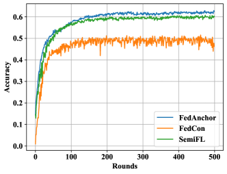
(b) IID ($Dir=1000$) - 10000 anchors

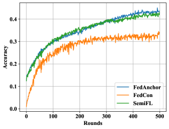
(c) non-IID ($Dir=0.1$) - 2500 anchors

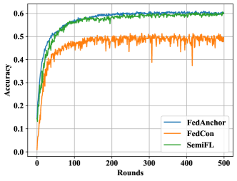
(d) non-IID ($Dir=0.1$) - 10000 anchors

Figure 7: Performance on CIFAR100 test set on ResNet-18 with both IID and non-IID cases across different numbers of anchor data setups, compared with the baseline.

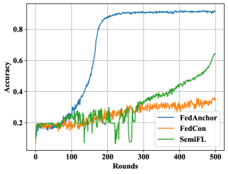
(a) IID ($Dir=1000$) - 250 anchors

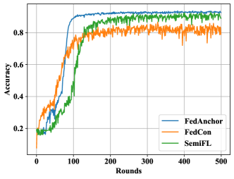
(b) IID ($Dir=1000$) - 1000 anchors

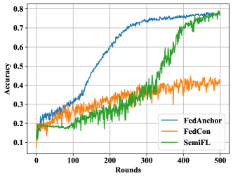
(c) non-IID ($Dir=0.1$) - 250 anchors

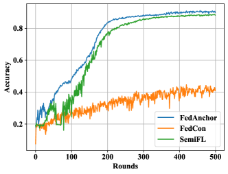
(d) non-IID ($Dir=0.1$) - 1000 anchors

Figure 8: Performance on SVHN test set on ResNet-18 with both IID and non-IID cases across different numbers of anchor data setups, compared with the baseline.

Appendix F Pseudo-labels quality plots

We compare our pseudo-label accuracy with one of the baseline (SemiFL) pseudo-label accuracy in Fig. 9. We generate the plot for different datasets and anchor sizes. In each plot, we provide the pseudo-label accuracy provided by the classification head and the pseudo-label accuracy provided by our anchor head. Since SemiFL does not have the anchor head, it only has one curve for each scenario. It is clear that FedAnchor produces significantly higher pseudo-label accuracy than the baseline. Hence, FedAnchor can achieve higher performance with a faster convergence rate. Fig. 1 (right) shows the pseudo-label accuracy at the round number 100, demonstrating that the FedAnchor can produce higher pseudo-label accuracy with a big margin.

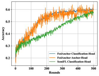
(a) CIFAR-10 non-IID ($Dir=0.1$) - 250 anchors

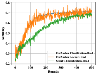
(b) CIFAR-10 non-IID ($Dir=0.1$) - 500 anchors

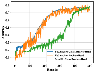
(c) SVHN non-IID ($Dir=0.1$) - 250 anchors

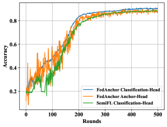
(d) SVHN non-IID ($Dir=0.1$) - 100 anchors

Figure 9: Comparison of the pseudo-label accuracy with one of the baseline (SemiFL) pseudo-label accuracy for both CIFAR10 and SVHN with different anchor sizes. Each plot shows the pseudo-label accuracy provided by the classification head and the pseudo-label accuracy provided by our anchor head. Since SemiFL does not have the anchor head, it only has one curve for each scenario.

Appendix G Implementation and reproducibility

During the extensive evaluation of FedAnchor, we adopted any means of making as reproducible as possible the experimental setting. Our code is publicly available in the anonymized repository at https://anonymous.4open.science/r/fedanchor-8727/README.md. The code could be easily executed in any machine possessing Nvidia GPUs. We used Poetry (https://python-poetry.org/) to create the Python package with its dependencies, such as PyTorch 2.1, Python 3.10, and Flower 1.5.0. This tool allows the researchers to reproduce the same environment that we used with minimal effort. Regarding the FedCon implementation, we followed the original repository (((zewei-long/fedcon-pytorch))).

References

- Bachman et al. (2014) Bachman, P., Alsharif, O., and Precup, D. Learning with pseudo-ensembles. Advances in neural information processing systems, 27, 2014.
- Berthelot et al. (2019) Berthelot, D., Carlini, N., Goodfellow, I., Papernot, N., Oliver, A., and Raffel, C. A. Mixmatch: A holistic approach to semi-supervised learning. Advances in neural information processing systems, 32, 2019.
- Beutel et al. (2020) Beutel, D. J., Topal, T., Mathur, A., Qiu, X., Fernandez-Marques, J., Gao, Y., Sani, L., Li, K. H., Parcollet, T., de Gusmão, P. P. B., et al. Flower: A friendly federated learning research framework. arXiv preprint arXiv:2007.14390, 2020.
- Chapelle et al. (2009) Chapelle, O., Scholkopf, B., and Zien, A. Semi-supervised learning (chapelle, o. et al., eds.; 2006)[book reviews]. IEEE Transactions on Neural Networks, 20(3):542–542, 2009.
- Cubuk et al. (2020) Cubuk, E. D., Zoph, B., Shlens, J., and Le, Q. V. Randaugment: Practical automated data augmentation with a reduced search space. In Proceedings of the IEEE/CVF conference on computer vision and pattern recognition workshops, pp. 702–703, 2020.
- Diao et al. (2022) Diao, E., Ding, J., and Tarokh, V. Semifl: Semi-supervised federated learning for unlabeled clients with alternate training. Advances in Neural Information Processing Systems, 35:17871–17884, 2022.
- Dimitriadis et al. (2020) Dimitriadis, D., Ken’ichi Kumatani, R. G., Gmyr, R., Gaur, Y., and Eskimez, S. E. A federated approach in training acoustic models. In Interspeech, pp. 981–985, 2020.
- Elbir et al. (2020) Elbir, A., Soner, B., and Coleri, S. Federated learning in vehicular networks. arxiv. arXiv preprint arXiv:2006.01412, 2020.
- French et al. (2017) French, G., Mackiewicz, M., and Fisher, M. Self-ensembling for visual domain adaptation. arXiv preprint arXiv:1706.05208, 2017.
- Gao et al. (2022a) Gao, Y., Fernandez-Marques, J., Parcollet, T., Mehrotra, A., and Lane, N. D. Federated self-supervised speech representations: Are we there yet? arXiv preprint arXiv:2204.02804, 2022a.
- Gao et al. (2022b) Gao, Y., Parcollet, T., Zaiem, S., Fernandez-Marques, J., de Gusmao, P. P., Beutel, D. J., and Lane, N. D. End-to-end speech recognition from federated acoustic models. In ICASSP 2022-2022 IEEE International Conference on Acoustics, Speech and Signal Processing (ICASSP), pp. 7227–7231. IEEE, 2022b.
- Grill et al. (2020) Grill, J.-B., Strub, F., Altché, F., Tallec, C., Richemond, P., Buchatskaya, E., Doersch, C., Avila Pires, B., Guo, Z., Gheshlaghi Azar, M., et al. Bootstrap your own latent-a new approach to self-supervised learning. Advances in neural information processing systems, 33:21271–21284, 2020.
- He et al. (2016) He, K., Zhang, X., Ren, S., and Sun, J. Deep residual learning for image recognition. In Proceedings of the IEEE conference on computer vision and pattern recognition, pp. 770–778, 2016.
- Hensel et al. (2021) Hensel, F., Moor, M., and Rieck, B. A survey of topological machine learning methods. Frontiers in Artificial Intelligence, 4:681108, 2021.
- Horvath et al. (2021) Horvath, S., Laskaridis, S., Almeida, M., Leontiadis, I., Venieris, S., and Lane, N. Fjord: Fair and accurate federated learning under heterogeneous targets with ordered dropout. Advances in Neural Information Processing Systems, 34:12876–12889, 2021.
- Jeong et al. (2020a) Jeong, W., Yoon, J., Yang, E., and Hwang, S. J. Federated semi-supervised learning with inter-client consistency & disjoint learning. arXiv preprint arXiv:2006.12097, 2020a.
- Jeong et al. (2020b) Jeong, W., Yoon, J., Yang, E., and Hwang, S. J. Federated semi-supervised learning with inter-client consistency & disjoint learning. arXiv preprint arXiv:2006.12097, 2020b.
- Jin et al. (2020) Jin, Y., Wei, X., Liu, Y., and Yang, Q. Towards utilizing unlabeled data in federated learning: A survey and prospective. arXiv preprint arXiv:2002.11545, 2020.
- Kornblith et al. (2019) Kornblith, S., Norouzi, M., Lee, H., and Hinton, G. Similarity of neural network representations revisited. In International conference on machine learning, pp. 3519–3529. PMLR, 2019.
- Krizhevsky (2012) Krizhevsky, A. Learning multiple layers of features from tiny images. University of Toronto, 05 2012.
- Lee (2013) Lee, D.-H. Pseudo-label : The simple and efficient semi-supervised learning method for deep neural networks. ICML 2013 Workshop : Challenges in Representation Learning (WREPL), 07 2013.
- Li et al. (2015) Li, Y., Yosinski, J., Clune, J., Lipson, H., and Hopcroft, J. Convergent learning: Do different neural networks learn the same representations? arXiv preprint arXiv:1511.07543, 2015.
- Lim et al. (2020) Lim, W. Y. B., Luong, N. C., Hoang, D. T., Jiao, Y., Liang, Y.-C., Yang, Q., Niyato, D., and Miao, C. Federated learning in mobile edge networks: A comprehensive survey. IEEE Communications Surveys & Tutorials, 22(3):2031–2063, 2020.
- Long et al. (2021) Long, Z., Wang, J., Wang, Y., Xiao, H., and Ma, F. Fedcon: A contrastive framework for federated semi-supervised learning. arXiv preprint arXiv:2109.04533, 2021.
- Mao et al. (2023) Mao, Y., Xiao, Z., Lin, C.-T., de Gusmão, P. P. B., Lane, N. D., Zach, C., and Alibeigi, M. Decentralized training of 3d lane detection with automatic labeling using hd maps. In 2023 IEEE 97th Vehicular Technology Conference (VTC2023-Spring), pp. 1–7. IEEE, 2023.
- McMahan et al. (2017) McMahan, B., Moore, E., Ramage, D., Hampson, S., and y Arcas, B. A. Communication-efficient learning of deep networks from decentralized data. In Artificial intelligence and statistics. PMLR, 2017.
- Moor et al. (2020) Moor, M., Horn, M., Rieck, B., and Borgwardt, K. Topological autoencoders. In International conference on machine learning, pp. 7045–7054. PMLR, 2020.
- Morcos et al. (2018) Morcos, A., Raghu, M., and Bengio, S. Insights on representational similarity in neural networks with canonical correlation. Advances in neural information processing systems, 31, 2018.
- Netzer et al. (2011) Netzer, Y., Wang, T., Coates, A., Bissacco, A., Wu, B., and Ng, A. Reading digits in natural images with unsupervised feature learning. NIPS, 01 2011.
- Nguyen & Yang (2023) Nguyen, K.-B. and Yang, J.-S. Boosting semi-supervised learning by bridging high and low-confidence predictions. arXiv preprint arXiv:2308.07509, 2023.
- Novotnỳ (2018) Novotnỳ, V. Implementation notes for the soft cosine measure. In Proceedings of the 27th ACM International Conference on Information and Knowledge Management, pp. 1639–1642, 2018.
- Qiu et al. (2022) Qiu, X., Fernandez-Marques, J., Gusmao, P. P., Gao, Y., Parcollet, T., and Lane, N. D. Zerofl: Efficient on-device training for federated learning with local sparsity. arXiv preprint arXiv:2208.02507, 2022.
- Qiu et al. (2023) Qiu, X., Parcollet, T., Fernandez-Marques, J., Gusmao, P. P., Gao, Y., Beutel, D. J., Topal, T., Mathur, A., and Lane, N. D. A first look into the carbon footprint of federated learning. Journal of Machine Learning Research, 24(129):1–23, 2023.
- Rasmus et al. (2015) Rasmus, A., Berglund, M., Honkala, M., Valpola, H., and Raiko, T. Semi-supervised learning with ladder networks. Advances in neural information processing systems, 28, 2015.
- Reddi et al. (2021) Reddi, S. J., Charles, Z., Zaheer, M., Garrett, Z., Rush, K., Konečný, J., Kumar, S., and McMahan, H. B. Adaptive federated optimization. In International Conference on Learning Representations, 2021.
- Rehman et al. (2022) Rehman, Y. A. U., Gao, Y., Shen, J., de Gusmao, P. P. B., and Lane, N. Federated self-supervised learning for video understanding. In European Conference on Computer Vision, pp. 506–522. Springer, 2022.
- Rehman et al. (2023) Rehman, Y. A. U., Gao, Y., de Gusmão, P. P. B., Alibeigi, M., Shen, J., and Lane, N. D. L-dawa: Layer-wise divergence aware weight aggregation in federated self-supervised visual representation learning. arXiv preprint arXiv:2307.07393, 2023.
- Sajjadi et al. (2016) Sajjadi, M., Javanmardi, M., and Tasdizen, T. Regularization with stochastic transformations and perturbations for deep semi-supervised learning. Advances in neural information processing systems, 29, 2016.
- Sohn et al. (2020) Sohn, K., Berthelot, D., Carlini, N., Zhang, Z., Zhang, H., Raffel, C. A., Cubuk, E. D., Kurakin, A., and Li, C.-L. Fixmatch: Simplifying semi-supervised learning with consistency and confidence. Advances in neural information processing systems, 33:596–608, 2020.
- Thulasidasan et al. (2019) Thulasidasan, S., Chennupati, G., Bilmes, J. A., Bhattacharya, T., and Michalak, S. On mixup training: Improved calibration and predictive uncertainty for deep neural networks. Advances in Neural Information Processing Systems, 32, 2019.
- Tsitsulin et al. (2019) Tsitsulin, A., Munkhoeva, M., Mottin, D., Karras, P., Bronstein, A., Oseledets, I., and Müller, E. The shape of data: Intrinsic distance for data distributions. arXiv preprint arXiv:1905.11141, 2019.
- Viala Bellander & Ghafir (2023) Viala Bellander, A. and Ghafir, Y. Towards federated fleet learning leveraging unannotated data. 2023.
- Vulić et al. (2020) Vulić, I., Ruder, S., and Søgaard, A. Are all good word vector spaces isomorphic? arXiv preprint arXiv:2004.04070, 2020.
- Yang et al. (2021) Yang, D., Xu, Z., Li, W., Myronenko, A., Roth, H. R., Harmon, S., Xu, S., Turkbey, B., Turkbey, E., Wang, X., et al. Federated semi-supervised learning for covid region segmentation in chest ct using multi-national data from china, italy, japan. Medical image analysis, 70:101992, 2021.
- Yang et al. (2022) Yang, X., Song, Z., King, I., and Xu, Z. A survey on deep semi-supervised learning. IEEE Transactions on Knowledge and Data Engineering, 2022.
- Zagoruyko & Komodakis (2016) Zagoruyko, S. and Komodakis, N. Wide residual networks. arXiv preprint arXiv:1605.07146, 2016.
- Zaheer et al. (2017) Zaheer, M., Kottur, S., Ravanbakhsh, S., Poczos, B., Salakhutdinov, R. R., and Smola, A. J. Deep sets. Advances in neural information processing systems, 30, 2017.
- Zhang et al. (2021) Zhang, Z., Yang, Y., Yao, Z., Yan, Y., Gonzalez, J. E., Ramchandran, K., and Mahoney, M. W. Improving semi-supervised federated learning by reducing the gradient diversity of models. In 2021 IEEE International Conference on Big Data (Big Data), pp. 1214–1225. IEEE, 2021.
- Zhou & Li (2005) Zhou, Z.-H. and Li, M. Tri-training: Exploiting unlabeled data using three classifiers. IEEE Transactions on knowledge and Data Engineering, 17(11):1529–1541, 2005.