Extracting randomness from quantum ‘magic’

Abstract

Magic is a critical property of quantum states that plays a pivotal role in fault-tolerant quantum computation. Simultaneously, random states have emerged as a key element in various randomized techniques within contemporary quantum science. In this study, we establish a direct connection between these two notions. More specifically, our research demonstrates that when a subsystem of a quantum state is measured, the resultant projected ensemble of the unmeasured subsystem can exhibit a high degree of randomness that is enhanced by the inherent ‘magic’ of the underlying state. We demonstrate this relationship rigorously for quantum state 2-designs, and present compelling numerical evidence to support its validity for higher-order quantum designs. Our findings suggest an efficient approach for leveraging magic as a resource to generate random quantum states.

The field of quantum computing has experienced remarkable advancements in recent decades Arute et al. (2019); Zhong et al. (2020); Bluvstein et al. (2024); Preskill (2018), yet the essential source of power driving the quantum speedup continues to be elusive. This complex issue is inherently multifaceted, with its resolution dependent on the theoretic framework for characterizing the underlying resources. For instance, entanglement was known to be insufficient — Clifford circuits produce entanglement among qubits but nevertheless can be efficiently simulated classically Gottesman (1998). On the flip side, the same set of operations constitutes the basic building block for the stabilizer formalism of quantum computing, which, when augmented with the so-called magic quantum states Bravyi and Kitaev (2005); Knill (2005); Campbell et al. (2012); Howard et al. (2014), makes a blueprint for universal fault tolerant quantum computation. This paradigm thus recognizes magic states as a crucial quantum resource. The exploration and exploitation of the physical properties of quantum magic states have recently emerged as an active area of research Veitch et al. (2014); Bravyi and Gosset (2016); Howard and Campbell (2017); Heinrich and Gross (2019); Bravyi et al. (2019); Wang et al. (2020); Heimendahl et al. (2021); Leone et al. (2022); Tirrito et al. (2023).

Randomness stands as another pivotal resource in quantum information science, playing a crucial role in numerous protocols for quantum information processing. Various applications, including quantum device benchmarking Arute et al. (2019); Cross et al. (2019); Neill et al. (2018); Harris et al. (2022); Wu et al. (2021), tomography Huang et al. (2020); Elben et al. (2023) and quantum channel approximation Hayden et al. (2004); Yan and Sinitsyn (2022); Kunjummen et al. (2023), rely on random quantum resources. In a recent breakthrough Cotler et al. (2023); Choi et al. (2023), it was demonstrated that random resources can be extracted from complex many-body quantum states. Specifically, when a subsystem of a strongly correlated many-body state undergoes projective measurements, the unmeasured subsystem yields a highly random quantum state ensemble, which nevertheless may not be directly prepared efficiently. This result not only offers an efficient protocol for generating random quantum states as a practical resource but also opens up new avenues for exploring fundamental physical problems, such as non-equilibrium quantum dynamics Ippoliti and Ho (2022); Lucas et al. (2023); Ippoliti and Ho (2023), and, as will be delved into in this work, characterization of quantum states.

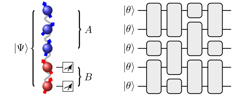
Figure 1: Left: A subsystem $B$ of a complex many-body state $|\Psi\rangle$ is subject to projective measurement. The unmeasured subsystem $A$ is projected to an ensemble of random states. Right: The qubits are prepared in a product magic state, parameterized by $\theta$, which is then tranformed by a random Clifford circuit, generating a state with the same magic value.

In this context, we unveil a profound connection between randomness and magic. Specifically, we demonstrate that typical quantum states exhibiting more magic yield post-measurement projected ensembles with greater randomness. The degree of magic and randomness are precisely quantified using proper metrics—namely, stabilizer Rényi entropy and quantum state $t$-design.

Significance of this result is two-fold: it proposes an efficient scheme for random quantum state generation with magic states and Clifford circuits. The later comprises operations that are naively fault tolerant in quantum computing architectures protected by stabilizer error-correcting codes, and therefore operationally “cost-free”. Simultaneously, on a conceptual level, it unravels an intrinsic randomness associated with magic quantum states. This randomness is a manifestation of many-body correlations that are not captured by conventional measures such as entanglement. Consequently, these findings shed new light on the role of magic as a quantum resource. In the following, we will lay down the essential components of the setup and present the main theorem, as well as supporting evidence from numerical simulations.

Projected ensemble.— For any ensemble of pure quantum states, $\mathcal{E}=\{(p_{i},|\psi_{i}\rangle)\}$, the level of its randomness can be quantified rigorously using the notion of quantum state design. Define the $t$-th moment of $\mathcal{E}$ as

$$\rho^{(t)}_{\mathcal{E}}=\sum_{i}p_{i}|\psi_{i}\rangle\langle\psi_{i}|^{\otimes t},$$ (1)

the average of its $t$-th tensor power, and denote especially the $t$-th moment of the Haar random ensemble by $\rho_{\text{Haar}}^{(t)}$. We say that $\mathcal{E}$ is a quantum state $t$-design if $\rho_{\mathcal{E}}^{(t)}=\rho_{\text{Haar}}^{(t)}$, that is, $\mathcal{E}$ is indistinguishable from Haar measure up to its $t$-th moment. In practice, an exact $t$-design can never be reached. It is therefore useful to have a measure of the approximate closeness of the ensemble’s distribution to the Haar measure. This idea is captured by an $\varepsilon$-approximate quantum state $t$-design, an ensemble $\mathcal{E}$ for which

$$d^{(t)}(\mathcal{E})\equiv||\rho_{\mathcal{E}}^{(t)}-\rho_{\text{Haar}}^{(t)}||\leq\varepsilon.$$ (2)

Here, $||\cdot||$ can be any proper norm over density matrices. Throughout this work, we will employ two commonly used norms, namely, trace norm $||\rho||_{1}\equiv\rm{tr}\sqrt{\rho^{\dagger}\rho}$ and the Hilbert-Schmidt norm $||\rho||_{2}\equiv\sqrt{\rm{tr}\rho^{\dagger}\rho}$, and denote the corresponding distance as $d^{(t)}_{\rm trace}(\mathcal{E})$ and $d^{(t)}_{\rm HS}(\mathcal{E})$, respectively.

A basic ingredient of our work is the use of a subsystem measurement to generate an ensemble of random states (Fig. 1, left). Consider a bipartite pure state $|\Psi\rangle\in\mathcal{H}_{AB}=\mathcal{H}_{A}\otimes\mathcal{H}_{B}$ over systems $A$ and $B$. We take the $A$ and $B$ subsytems to be composed of $N_{A}$ and $N_{B}$ qubits, respectively. Denote $N\equiv N_{A}+N_{B}$, $d_{A}\equiv 2^{N_{A}}$, $d_{B}\equiv 2^{N_{B}}$, and $d\equiv 2^{N}$, and let $\{|i\rangle_{B}\}_{i=1}^{d_{B}}$ be a basis of product states for $\mathcal{H}_{B}$. The outcomes of a projective measurement on the $B$ subsystem with respect to this basis, followed by a discarding of the $B$ subsystem, form an ensemble of states $\mathcal{E}_{|\Psi\rangle}\equiv\{(p_{i},|\psi_{i}\rangle)\}$ on the $A$ subsystem, where the probability $p_{i}$ is

$$p_{i}=\langle\Psi|(I_{A}\otimes|i\rangle\langle i|_{B})|\Psi\rangle$$ (3)

and the corresponding projected state of $A$ is

$$|\psi_{i}\rangle=(I_{A}\otimes\langle i|_{B})|\Psi\rangle/\sqrt{p_{i}}.$$ (4)

We will refer to the ensemble $\mathcal{E}_{|\Psi\rangle}$ as the projected ensemble generated by $|\Psi\rangle$. One can quantify this ensemble using the notion of a $t$-design discussed above.

Conceivably, distribution of the projected ensemble reflects the intrinsic randomness of the underlying generating state; a more complex many-body state, e.g., with stronger entanglement, may produce a projected ensemble with a higher degree of randomness. Indeed, this intuition was captured formally in a recent result in Cotler et al. (2023); Choi et al. (2023), that is, if the pre-measurement state $|\Psi\rangle$ itself was sampled from an $\varepsilon^{\prime}$-approximate $t^{\prime}$-design (greater $t^{\prime}$ indicates higher complexity), the projected ensemble $\mathcal{E}_{|\Psi\rangle}$ will form an $\varepsilon$-approximate $t$-design with probability $1-\delta$ for any positive $\varepsilon,\delta$, and integer $t\geq 1$, given that $N_{A}$ and $N_{B}$ are sufficiently large. This provides an efficient scheme for generating random state ensembles from a single (complex) many-body state with projective measurement without having to sample from random quantum circuit realizations, as in the conventional approach.

Magic states.—The notion of magic states stems from the stabilizer formalism of fault-tolerant quantum computing. The latter was built upon a finite and non-universal set of unitary operations, the Clifford gates. Due to their non-universality, quantum circuits consisting of only Clifford operations can only produce a proper subset of all quantum states (from a fixed initial state). States that cannot be produced by Clifford circuits applied on initial computational basis states are called non-stabilizer states. Remarkably, it is known that by supplementing stabilizer operations with certain non-stabilizer states, one may achieve universal quantum computation. The degree of non-stabilizerness of a state is typically referred to as its “magic,” and may be quantified by various measures Veitch et al. (2014); Bravyi and Gosset (2016); Howard and Campbell (2017); Heinrich and Gross (2019); Bravyi et al. (2019); Wang et al. (2020); Heimendahl et al. (2021). Here, we employ a recently developed measure for magic, the stabilizer linear entropy Leone et al. (2022).

More precisely, denote by $\mathcal{P}_{n}$ the set of all tensor products $P_{1}\otimes\dots\otimes P_{n}$ where $P_{i}$ is a single qubit Pauli operator for $1\leq i\leq n$. Note that $\mathcal{P}_{n}$ is merely the set of all Pauli strings on $n$ systems and not the whole Pauli group, which includes global phase factors of $\pm 1,\pm i$. For any given state $|\psi\rangle$ over $n$ qubits and Pauli string $P\in\mathcal{P}_{n}$, define $\Xi_{P}(|\psi\rangle)\equiv\frac{1}{2^{n}}\langle\psi|P|\psi\rangle^{2}$, the (normalized) square of the expectation value of $P$ over state $|\psi\rangle$. From this, we may define the vector $\Xi(|\psi\rangle)\equiv(\Xi_{P}(|\psi\rangle))_{P\in\mathcal{P}_{n}}$, which has $4^{n}$ real components. The stabilizer linear entropy is defined to be

$$M_{\rm lin}(|\psi\rangle)=1-2^{n}|\Xi(|\psi\rangle)|_{2}^{2},$$ (5)

where $|\cdot|_{2}$ is simply the Euclidean norm on $\mathbb{R}^{4^{n}}$. This measure satisfies the properties desired for good measures of nonstabilizerness from the point of view of resource theory Leone et al. (2022) and offers the computational advantages for the purpose of the present work.

Connecting magic and randomness.—We are now ready to establish the link between magic and randomness. Suppose that we generate an ensemble $\mathcal{E}_{|\Psi\rangle}$ from a state $|\Psi\rangle$ via the subsystem measurement introduced above. One might ask how the randomness of the resulting projected ensemble, as measured by distance $d^{(t)}(\mathcal{E}_{|\Psi\rangle})$ in (2), depends on the magic of state $|\Psi\rangle$, as quantified by the stabilizer linear entropy $M_{\rm lin}(|\Psi\rangle)$ in (5). However, this query is ill-posed because different states of the same magic value may produce very different levels of randomness. A more fruitful approach is to quantify the relationship between a particular value of magic $M$ and the randomness $d^{(t)}(\mathcal{E}_{|\Psi\rangle})$ of the projected ensemble averaged over all states $|\Psi\rangle$ with the same magic value $M$. A crucial feature of the stabilizer linear entropy (and any other sensible measure of magic) is that it does not change under Clifford operations, which are “cost-free” from an operational point of view. This therefore allows us to evaluate the average with respect to all unitaries in the Clifford group, i.e.,

$$\left\langle d^{(t)}(\mathcal{E}_{C|\Psi\rangle})\right\rangle_{\mathcal{C}_{N}}\equiv\int_{C\in\mathcal{C}_{N}}dC~{}d^{(t)}(C|\Psi\rangle),$$ (6)

where $\mathcal{C}_{N}$ is the Clifford group of $N$ qubits. The task is then to determine the relationship between $\left\langle d^{(t)}(\mathcal{E}_{C|\Psi\rangle})\right\rangle_{\mathcal{C}_{N}}$ and $M_{\rm lin}(|\Psi\rangle)$. This leads to the key result of this study.

Theorem 1

Up to an error that decays exponentially with respect to $N_{A}$ and $N_{B}$, the average randomness extracted from $|\Psi\rangle$ is described by

$$\begin{split}\left\langle[d_{\rm HS}^{(2)}(\mathcal{E}_{C|\Psi\rangle})]^{2}\right\rangle_{\mathcal{C}_{N}}&=\alpha-\beta M_{\rm lin}(|\Psi\rangle)+\varepsilon,\end{split}$$ (7)

where $\alpha$ and $\beta$ are numerical factors that depend on both subsystem dimensions, and

$$\frac{|\varepsilon|}{\left\langle[d_{\rm HS}^{(2)}(\mathcal{E}_{C|\Psi\rangle})]^{2}\right\rangle_{\mathcal{C}_{N}}}=\Theta\bigg{(}\frac{1}{d_{A}}\bigg{)}.$$ (8)

For the proof, see Supplementary Material (SM). We add that we consider the average of the square of $d_{\rm HS}^{(2)}(\mathcal{E}_{C|\Psi\rangle})$ rather than the Hilbert-Schmidt distance itself because doing so allows us to avoid the difficulty of averaging the square root of the operator trace, and hence deduce a rigorous result. The average-of-square $\langle[d_{\rm HS}^{(2)}(\mathcal{E}_{C|\Psi\rangle})]^{2}\rangle_{\mathcal{C}_{N}}$ is expected to approximate the square-of-average $\langle d_{\rm HS}^{(2)}(\mathcal{E}_{C|\Psi\rangle})\rangle^{2}_{\mathcal{C}_{N}}$ for large systems due to concentration of measure, with an error suppressed exponentially fast with the system size.

This theorem implies a direct connection between the randomness one may extract from quantum states and their magic. It gives a new meaning to the stabilizer linear entropy of an arbitrary state in terms of the extractable randomness from that state. Furthermore, since the coefficients tend to zero as $d_{A},d_{B}\to\infty$, Theorem 1 confirms that as one increases the size of the subsystem measurement and of the surviving systems, the values of $d_{\rm HS}^{(2)}(\mathcal{E}_{C|\Psi\rangle})$ tend to zero, i.e., the randomness becomes near perfect.

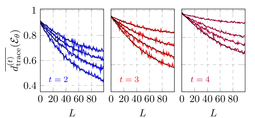
Figure 2: We numerically estimate $\overline{d^{(t)}_{\mathrm{trace}}}(\mathcal{E}_{\theta})$, or the average normalized trace distance between the $t$-th moments of the Haar ensemble and the projected ensembles with $N_{A}=2$ and $N_{B}=4$ obtained from the output of a random Clifford circuit of finite depth. For each circuit depth, the numerical average is taken over 100 realizations of a random Clifford circuit of the given depth initialized to $|\Psi(\theta)\rangle$. We plot $\overline{d^{(t)}_{\mathrm{trace}}}(\mathcal{E}_{\theta})$ as a function of circuit depth assuming initial states $|\Psi(\theta)\rangle$ of magic value $M_{\mathrm{lin}}(|\Psi(\theta)\rangle)=0,0.25,0.5,0.75$, with lower curves corresponding to higher magic values. The numerically simulated values are fitted to an exponential curve of best fit (black solid line).

Simulations.— Due to the rapid growth in the size of the Clifford group $\mathcal{C}_{N}$ with respect to $N$, it is difficult to numerically compute our quantifier of randomness $\left\langle d^{(t)}(\mathcal{E}_{C|\Psi\rangle})\right\rangle_{\mathcal{C}_{N}}$. To circumvent this issue, we estimate $\left\langle d^{(t)}(\mathcal{E}_{|C\Psi\rangle})\right\rangle_{\mathcal{C}_{N}}$ by averaging across random Clifford circuits of restricted length and extrapolating the results. Furthermore, another advantage of considering simulations of random Clifford circuits together with subsystem measurements is that they represent a physical quantum information processing task in which nonstabilizerness can affect the formation of approximate state designs.

We consider an $N$-qubit product state $|\Psi(\theta)\rangle=2^{-N/2}(|0\rangle+e^{i\theta}|1\rangle)^{\otimes N}$, which has a magic value $M_{\text{lin}}(|\Psi(\theta)\rangle)=1-(1+\cos^{4}{\theta}+\sin^{4}{\theta})^{N}/d$ Tirrito et al. (2023). The state $|\Psi(\theta)\rangle$ is evolved according to a random Clifford circuit $C_{L}=\prod_{i=1}^{L}U_{i}$ of depth $L$. Each layer $U_{i}$ of this circuit (Fig. 1, right) acts on two registers randomly sampled from the $N$ total registers and is itself randomly selected from the two-qubit gate set $\{\text{CNOT},H\otimes I,S\otimes I$, $I\otimes H$, $I\otimes S$}, where $H$ is the Hadamard gate and $S=\text{diag}(1,\ e^{i\pi/4})$ is the phase shift gate. The projected ensemble $\mathcal{E}_{C_{L}|\Psi(\theta)\rangle}$ over the $A$ subsystem is then obtained by simulating projective measurements on the state $C_{L}|\Psi(\theta)\rangle$ over the $B$ subsystem. Define $\overline{d_{\rm trace}^{(t)}}(\mathcal{E}_{\theta})$ to be the average of $d_{\rm trace}^{(t)}(\mathcal{E}_{C_{L}|\Psi(\theta)\rangle})/2$ over all possible Clifford circuits $C_{L}$ of depth $L$ composed of two qubit unitaries in the previously described manner. Here, we insert a normalization factor of $1/2$ to ensure that $\overline{d_{\rm trace}^{(t)}}(\mathcal{E}_{\theta})$ lies in $[0,1]$ for illustrative purposes. We emphasize that the bar is used to indicate an average over all Clifford circuits of a specified length, rather than the entire Clifford group as in (6). A numerical estimate for the trace distance $\overline{d_{\text{trace}}^{(t)}}(\mathcal{E}_{\theta})$ is obtained by averaging over many realizations of a random Clifford circuit. By varying the depth of the simulated circuit, we obtain data for $\overline{d_{\text{trace}}^{(t)}}(\mathcal{E}_{\theta})$ as a function of circuit depth $L$.

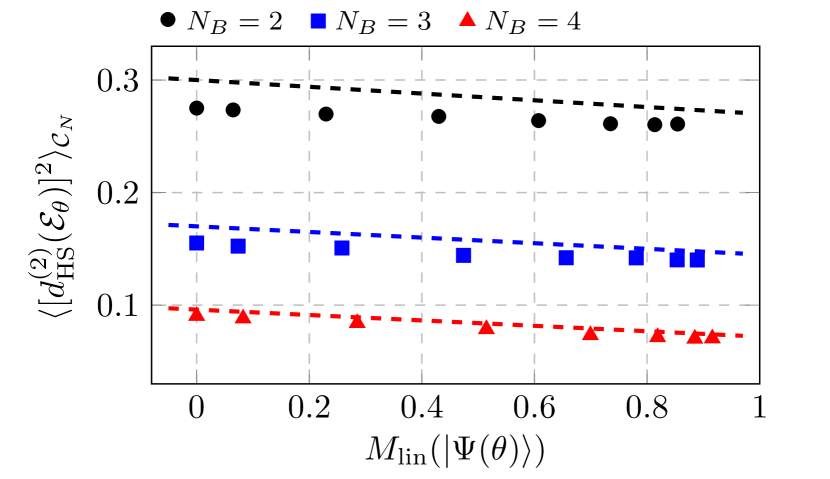
Figure 3: We plot a numerical estimate for the average extracted second degree randomness $\langle[d_{\mathrm{HS}}^{(2)}(\mathcal{E}_{\theta})]^{2}\rangle_{C_{N}}$ of the initial state $|\Psi(\theta)\rangle$ as a function of its magic value $M_{\mathrm{lin}}(|\Psi(\theta)\rangle)$ (points). We also plot our analytic approximation (7) for $\langle[d_{\mathrm{HS}}^{(2)}(\mathcal{E}_{\theta})]^{2}\rangle_{C_{N}}$ as a function of $M_{\mathrm{lin}}(|\Psi(\theta)\rangle)$ (dashed line). Numerical estimates for $\langle[d_{\mathrm{HS}}^{(2)}(\mathcal{E}_{\theta})]^{2}\rangle_{C_{N}}$ were obtained by extrapolating averages of $[d_{\mathrm{HS}}^{(2)}(\mathcal{E}_{C_{L}|\Psi(\theta)\rangle})]^{2}$ across 100 realizations per circuit depth of random Clifford circuits, with depth ranging from 1 to 200. All results were obtained for $N_{A}=5$, with black circle, blue square, and red triangle corresponding to $N_{B}=2,3,$ and $4$, respectively.

Numerically, we see that the average distance $\overline{d_{\text{trace}}^{(2)}}(\mathcal{E}_{\theta})$ of the post-measurement ensemble decays exponentially with respect to the circuit depth $L$, with values of $\theta$ corresponding to a higher magic value producing a faster decay (Fig. 2). The variation in the decay curves shows that the magic of many-body quantum states influences the degree of randomness that may be extracted from them via local measurements. Furthermore, it was observed that the asymptotic value of the decay in average trace distance falls exponentially with respect to $N_{B}$ for fixed $N_{A}$ and magic, while it decreases linearly with respect to $M_{\text{lin}}(|\Psi(\theta)\rangle)$ for fixed $N_{A}$ and $N_{B}$. The latter is consistent with Theorem 1 (see ).

The exponential decay of the $\overline{d_{\rm trace}^{(t)}}(\mathcal{E}_{\theta})$ with respect to circuit depth may be seen as a general property of random circuits: For many random circuit configurations, the behavior of $d^{(t)}(\mathcal{E})$ has been studied Brandao et al. (2016); Harrow and Low (2009), where in this case $\mathcal{E}$ is the ensemble of all possible states that may be evolved from a fixed initial state of the random circuit. Generally, any positive value $\varepsilon$ of $d^{(t)}(\mathcal{E})$ may be achieved provided the circuit depth $L$ scales at least linearly with respect to $t$, number of registers $N$, and $\log(1/\varepsilon)$. The linear growth of this threshold with respect to $\log(1/\varepsilon)$ suggests that $d^{(t)}(\mathcal{E})$ decays exponentially with respect to circuit depth in these random circuit paradigms. Since the measurements in our scheme introduce an extra degree of randomness, our value of $\overline{d^{(t)}}(\mathcal{E}_{\theta})$ should decay at least exponentially fast, as was observed numerically. Furthermore, the exponential decay of the asymptotic values with respect to $N_{B}$ follow from Theorem 2 of Ref. Cotler et al. (2023), where the bounds on the value of $N_{B}$ necessary to produce a post-measurement ensemble $\mathcal{E}$ with a value of $d_{\rm trace}^{(t)}(\mathcal{E})\leq\varepsilon$ require that $N_{B}$ scale exponentially faster than $\log(1/\varepsilon)$.

We conclude our numerical study with a demonstration of Theorem 1. As before, we define $\overline{(d_{\rm HS}^{(t)})^{2}}(\mathcal{E}_{\theta})$ to be the average of $[d_{\rm HS}^{(t)}(\mathcal{E}_{C_{L}|\Psi(\theta)\rangle})]^{2}$ over all possible Clifford circuits $C_{L}$ of depth $L$ composed according to the aformentioned two-qubit gate prescription. By numerically estimating $\overline{(d_{\rm HS}^{(t)})^{2}}(\mathcal{E}_{\theta})$ with many iterations of a finite-depth Clifford circuit, we obtain data for the exponential decay of $\overline{(d_{\rm HS}^{(t)})^{2}}(\mathcal{E}_{\theta})$ as a function of circuit depth. Fitting this data to an exponential decay function, we are able to extrapolate to infinite depth so that we obtain an approximation for $\langle[d_{\rm HS}^{(t)}(\mathcal{E}_{C|\Psi(\theta)\rangle})]^{2}\rangle_{\mathcal{C}_{N}}$, which we abbreviate to $\langle[d_{\rm HS}^{(t)}(\mathcal{E}_{\theta})]^{2}\rangle_{\mathcal{C}_{N}}$. By repeating this process for various angles of $\theta$, we are able to obtain $\langle[d_{\rm HS}^{(t)}(\mathcal{E}_{\theta})]^{2}\rangle_{\mathcal{C}_{N}}$ as a function of $M_{\rm lin}(|\Psi(\theta)\rangle)$, as seen in Fig. 3 for $t=2$. Note the linear nature of the relationship between $\langle[d_{\rm HS}^{(2)}(\mathcal{E}_{\theta})]^{2}\rangle_{\mathcal{C}_{N}}$ and magic. Furthermore, the numerically simulated values for $\langle[d_{\rm HS}^{(2)}(\mathcal{E}_{\theta})]^{2}\rangle_{\mathcal{C}_{N}}$ fall below those of the plotted analytical approximation (7). We have numerically verified that these data fall within the error threshold given by (8). Further analysis shows that we can expect the deviation between the values of $\langle[d_{\rm HS}^{(2)}(\mathcal{E}_{\theta})]^{2}\rangle_{\mathcal{C}_{N}}$ and its analytical approximation to be uniformly negative (see the SM).

Discussion.— One of the most notable aspects of this study is the transformative influence of the magic inherent in the initial state on the resulting randomness in the projected ensemble. It is crucial to stress that the Clifford group constitutes a quantum unitary $3$-design Zhu (2017). This implies that the produced ensemble (of the total system before projective measurement) by random Clifford circuits forms a quantum state $3$-design as well, irrespective with the initial input state. Consequently, one might naturally anticipate that the projected ensemble’s randomness level should be independent of the initial state, contrary to our observation.

The observed augmentation of the randomness level of the projected ensemble due to the amount of magic reflects internal correlations among subsystems within each single quantum state of the ensemble. These correlations go beyond what conventional metrics can capture. For example, entanglement of bipartite pure quantum states are completely determined by the reduced density matrix of the subsystems Horodecki et al. (2009), representing a first-moment average of the projected ensemble [$t=1$ in (1)]. The connection between magic and randomness thus suggests a novel approach for characterizing and harnessing correlations in magic states.

Simultaneously, leveraging the benefits of high-order quantum state designs necessitates multiple copies of each states within the ensemble. This poses a significant constraint on the precision of random state generation protocols, challenging both the conventional method such as sampling random unitary circuits and the recently proposed projected ensemble approach. The strategy proposed in this work, involving the use of Clifford circuits, marks a crucial first step toward developing a fault tolerant protocol for random state generation.

Acknowledgement.—This work was supported in part by the U.S. Department of Energy, Office of Science, Office of Advanced Scientific Computing Research, through the Quantum Internet to Accelerate Scientific Discovery Program, and in part by the LDRD program at Los Alamos. C.V. also acknowledges support from the Quantum Computing Summer School at Los Alamos National Laboratory.

Supplemental Material for
Extracting randomness from quantum ‘magic’

Here we present the proof of Theorem 1 in the main text.

Appendix A Overall picture

Fix $|\psi\rangle\in\mathcal{H}_{A}\otimes\mathcal{H}_{B}$ and define $P_{i}\equiv I_{A}\otimes|i\rangle\langle i|_{B}$ for each bit string $i\in\{0,1\}^{N_{B}}$. For any Clifford unitary $C\in\mathcal{C}_{N}$, we define $\rho_{C}^{(2)}$ to be the second moment of the post-measurement ensemble obtained from the generator state $C|\psi\rangle$:

$$\rho_{C}^{(2)}=\sum_{i\in\{0,1\}^{N_{B}}}\frac{\text{Tr}_{B}[P_{i}C\psi C^{\dagger}P_{i}]^{\otimes 2}}{\text{Tr}[P_{i}C\psi C^{\dagger}]}.$$ (9)

We wish to calculate

$$\begin{split}\langle\|\rho_{C}^{(2)}-\rho_{H}^{(2)}\|_{2}^{2}\rangle_{\mathcal{C}_{N}}&=\langle\text{Tr}[(\rho_{C}^{(2)}-\rho_{H}^{(2)})^{2}]\rangle_{\mathcal{C}_{N}}\\ &=\langle\text{Tr}[(\rho_{C}^{(2)})^{2}]\rangle_{\mathcal{C}_{N}}-2\langle\text{Tr}[\rho_{C}^{(2)}\rho_{H}^{(2)}]\rangle_{\mathcal{C}_{N}}+\text{Tr}[(\rho_{H}^{(2)})^{2}]\\ &=(\textnormal{I})-2(\textnormal{II})+(\textnormal{III}).\end{split}$$ (10)

Define $d=2^{N}$. Let $\mathcal{P}_{N}$ be the set of all tensor products of Pauli operators over $N$ qubits, and for all $P\in\mathcal{P}_{N}$ define $\Xi_{P}(|\psi\rangle)=d^{-1}\langle\psi|P|\psi\rangle^{2}$. Then construct the $4^{N}$-component vector $\Xi(|\psi\rangle)=(\Xi_{P}(|\psi\rangle))_{P\in\mathcal{P}_{N}}$. The stabilizer linear entropy is defined as

$$M_{\rm lin}(|\psi\rangle)=1-d\|\Xi(|\psi\rangle)\|_{2}^{2}.$$ (11)

Our ultimate goal is to express (10) as a function of the nonstabilizerness of $|\psi\rangle$. The metric of nonstabilizerness that we will use is the stabilizer linear entropy. In what follows, we assume that $d_{A}\equiv 2^{N_{A}},d_{B}\equiv 2^{N_{B}}\gg 1$.

A.1 Evaluation of Term 1

We will evaluate each term in (10) individually, starting with term I. We have

$$\begin{split}\langle\text{Tr}[(\rho_{C}^{(2)})^{2}]\rangle_{\mathcal{C}_{N}}&=\bigg{\langle}\text{Tr}\bigg{\{}\sum_{i,j\in\{0,1\}^{N_{B}}}\frac{\text{Tr}_{B}[P_{i}C\psi C^{\dagger}P_{i}]^{\otimes 2}}{\text{Tr}[P_{i}C\psi C^{\dagger}]}\frac{\text{Tr}_{B}[P_{j}C\psi C^{\dagger}P_{j}]^{\otimes 2}}{\text{Tr}[P_{j}C\psi C^{\dagger}]}\bigg{\}}\bigg{\rangle}_{\mathcal{C}_{N}}\\ &=\sum_{i,j\in\{0,1\}^{N_{B}}}\bigg{\langle}\frac{\text{Tr}[S_{A}([P_{i}C\psi C^{\dagger}P_{i}]^{\otimes 2}\otimes[P_{j}C\psi C^{\dagger}P_{j}]^{\otimes 2})]}{\text{Tr}[(P_{i}C\psi C^{\dagger})\otimes(P_{j}C\psi C^{\dagger})]}\bigg{\rangle}_{\mathcal{C}_{N}}\\ &=\sum_{i,j\in\{0,1\}^{N_{B}}}\bigg{\langle}\frac{\text{Tr}[S_{A}([P_{i}^{\otimes 2}\otimes P_{j}^{\otimes 2}][C^{\otimes 4}\psi^{\otimes 4}C^{\dagger\otimes 4}][P_{i}^{\otimes 2}\otimes P_{j}^{\otimes 2}])]}{\text{Tr}[(P_{i}\otimes P_{j})(C^{\otimes 2}\psi^{\otimes 2}C^{\dagger\otimes 2})]}\bigg{\rangle}_{\mathcal{C}_{N}}\\ &\approx\sum_{i,j\in\{0,1\}^{N_{B}}}\frac{\langle\text{Tr}[S_{A}([P_{i}^{\otimes 2}\otimes P_{j}^{\otimes 2}][C^{\otimes 4}\psi^{\otimes 4}C^{\dagger\otimes 4}][P_{i}^{\otimes 2}\otimes P_{j}^{\otimes 2}])]\rangle_{\mathcal{C}_{N}}}{\langle\text{Tr}[(P_{i}\otimes P_{j})(C^{\otimes 2}\psi^{\otimes 2}C^{\dagger\otimes 2})]\rangle_{\mathcal{C}_{N}}}\\ &=\sum_{i,j\in\{0,1\}^{N_{B}}}\frac{\text{Tr}[S_{A}([P_{i}^{\otimes 2}\otimes P_{j}^{\otimes 2}]\langle C^{\otimes 4}\psi^{\otimes 4}C^{\dagger\otimes 4}\rangle_{\mathcal{C}_{N}}[P_{i}^{\otimes 2}\otimes P_{j}^{\otimes 2}])]}{\text{Tr}[(P_{i}\otimes P_{j})\langle C^{\otimes 2}\psi^{\otimes 2}C^{\dagger\otimes 2}\rangle_{\mathcal{C}_{N}}]},\end{split}$$ (12)

where the numerators in the above expressions are a function of operators over a fourfold copy of the Hilbert space $\mathcal{H}_{A}\otimes\mathcal{H}_{B}$, and $S_{A}$ is the swap operator acting on the $A$ parts of these Hilbert spaces across the partition $12|34$. The justification for the approximation on the fourth line is given below in the subsection titled “Mean Quotient Approximation for Term I.”

A.1.1 Evaluation of Denominator

Let us calculate the denominator of the expression in (12) first. Since the uniformly-weighted Clifford group forms a 2-design, we automatically have

$$\langle C^{\otimes 2}\psi^{\otimes 2}C^{\dagger\otimes 2}\rangle_{\mathcal{C}_{N}}=\frac{\Pi_{2}^{sym}}{\text{Tr}[\Pi_{2}^{sym}]},$$ (13)

where for all $k>1$, we define $\Pi_{k}^{sym}=\sum_{\rho\in S_{k}}T_{\rho}$, with $T_{\rho}$ being the operator over $(\mathcal{H}_{A}\otimes\mathcal{H}_{B})^{\otimes k}$ that permutes the $k$ tensor factors in this space according to the permutation $\rho$. The operator $\Pi_{k}^{sym}$ is the unnormalized projector onto the symmetric subspace of $(\mathcal{H}_{A}\otimes\mathcal{H}_{B})^{\otimes k}$, and has trace given by $\text{Tr}[\Pi_{k}^{sym}]=d(d+1)\dots(d+k-1)$. Note that permutations over $(\mathcal{H}_{A}\otimes\mathcal{H}_{B})^{\otimes k}$ factor as $T_{\rho}=T_{\rho}^{A}\otimes T_{\rho}^{B}$, where $T_{\rho}^{A}$ and $T_{\rho}^{B}$ are the operators corresponding to the action of the permutation $\rho\in S_{k}$ over $\mathcal{H}_{A}^{\otimes k}$ and $\mathcal{H}_{B}^{\otimes k}$, respectively. We then have

$$\begin{split}\text{Tr}[(P_{i}\otimes P_{j})\langle C^{\otimes 2}\psi^{\otimes 2}C^{\dagger\otimes 2}\rangle_{\mathcal{C}_{N}}]&=\sum_{\rho\in S_{2}}\frac{\text{Tr}[([I_{A}\otimes|i\rangle\langle i|_{B}]\otimes[I_{A}\otimes|j\rangle\langle j|_{B}])(T_{\rho}^{A}\otimes T_{\rho}^{B})]}{d_{A}d_{B}(d_{A}d_{B}+1)}\\ &=\sum_{\rho\in S_{2}}\frac{\text{Tr}[T_{\rho}^{A}\otimes([|i\rangle\langle i|_{B}\otimes|j\rangle\langle j|_{B}]T_{\rho}^{B})]}{d_{A}d_{B}(d_{A}d_{B}+1)}\\ &=\sum_{\rho\in S_{2}}\frac{\text{Tr}[T_{\rho}^{A}]\langle ij|_{B}T_{\rho}^{B}|ij\rangle_{B}}{d_{A}d_{B}(d_{A}d_{B}+1)}\\ &=\begin{cases}\frac{\text{Tr}[T_{\text{Id}}^{A}]\langle ij|_{B}T_{\text{Id}}^{B}|ij\rangle_{B}}{d_{A}d_{B}(d_{A}d_{B}+1)},&i\neq j\\ \sum_{\rho\in S_{2}}\frac{\text{Tr}[T_{\rho}^{A}]}{d_{A}d_{B}(d_{A}d_{B}+1)},&i=j\end{cases}\\ &=\begin{cases}\frac{d_{A}}{d_{B}(d_{A}d_{B}+1)}&i\neq j\\ \frac{d_{A}+1}{d_{B}(d_{A}d_{B}+1)}&i=j\end{cases}\end{split}$$ (14)

A.1.2 Rewriting the Numerator

We now calculate the numerator of (12). By a result of Leone et al., we have that

$$\begin{split}\langle C^{\otimes 4}\psi^{\otimes 4}C^{\dagger\otimes 4}\rangle_{\mathcal{C}_{N}}&=aQ\Pi_{4}^{sym}+b\Pi_{4}^{sym},\end{split}$$ (15)

where

$$\begin{split}&a=\frac{\|\Xi(|\psi\rangle)\|_{2}^{2}}{4(d_{A}d_{B}+1)(d_{A}d_{B}+2)}-b\\ &b=\frac{1-\|\Xi(|\psi\rangle)\|_{2}^{2}}{(d_{A}^{2}d_{B}^{2}-1)(d_{A}d_{B}+2)(d_{A}d_{B}+4)}\\ &Q=\frac{1}{d_{A}^{2}d_{B}^{2}}\sum_{P\in\mathcal{P}_{N}}P^{\otimes 4}.\end{split}$$ (16)

In this instance, $\mathcal{P}_{N}$ simply denotes the set of tensor products of Pauli operators of length $N$, not the entire Pauli group on $N$ qubits (i.e., it does not include phase prefactors). The numerator of the expression in (12) becomes

$$\begin{split}\text{Tr}[S_{A}([P_{i}^{\otimes 2}\otimes P_{j}^{\otimes 2}]\langle C^{\otimes 4}\psi^{\otimes 4}C^{\dagger\otimes 4}\rangle_{\mathcal{C}_{N}}[P_{i}^{\otimes 2}\otimes P_{j}^{\otimes 2}])]&=a\text{Tr}[S_{A}([P_{i}^{\otimes 2}\otimes P_{j}^{\otimes 2}]Q\Pi_{4}^{sym}[P_{i}^{\otimes 2}\otimes P_{j}^{\otimes 2}])]\\ &+b\text{Tr}[S_{A}([P_{i}^{\otimes 2}\otimes P_{j}^{\otimes 2}]\Pi_{4}^{sym}[P_{i}^{\otimes 2}\otimes P_{j}^{\otimes 2}])].\end{split}$$ (17)

A.1.3 Evaluation of Second Numerator Term

We evaluate the latter term of the numerator (17) first. If $i\neq j$, one has

$$\begin{split}\text{Tr}[S_{A}([P_{i}^{\otimes 2}\otimes P_{j}^{\otimes 2}]\Pi_{4}^{sym}[P_{i}^{\otimes 2}\otimes P_{j}^{\otimes 2}])]&=\sum_{\rho\in S_{4}}\text{Tr}[S_{A}([P_{i}^{\otimes 2}\otimes P_{j}^{\otimes 2}]T_{\rho}[P_{i}^{\otimes 2}\otimes P_{j}^{\otimes 2}])]\\ &=\sum_{\rho\in S_{4}}\text{Tr}[S_{A}([(I_{A}\otimes|i\rangle\langle i|_{B})^{\otimes 2}\otimes(I_{A}\otimes|j\rangle\langle j|_{B})^{\otimes 2}]\\ &\ \ \ \ \ \ \ \ \ \ \ \ \times[T_{\rho}^{A}\otimes T_{\rho}^{B}][(I_{A}\otimes|i\rangle\langle i|_{B})^{\otimes 2}\otimes(I_{A}\otimes|j\rangle\langle j|_{B})^{\otimes 2}])]\\ &=\sum_{\rho\in S_{4}}\text{Tr}[S_{A}(T_{\rho}^{A}\otimes|iijj\rangle\langle iijj|_{B}T_{\rho}^{B}|iijj\rangle\langle iijj|_{B})]\\ &=\sum_{\rho\in\{\text{Id},(12),(34),(12)(34)\}}\text{Tr}[S_{A}(T_{\rho}^{A}\otimes|iijj\rangle\langle iijj|_{B})]\\ &=\sum_{\rho,\sigma\in S_{2}}\text{Tr}[(S_{A}[T_{\rho}^{A,12}\otimes T_{\sigma}^{A,34}])\otimes|iijj\rangle\langle iijj|_{B}]\\ &=\sum_{\rho,\sigma\in S_{2}}\text{Tr}[S_{A}(T_{\rho}^{A,12}\otimes T_{\sigma}^{A,34})]\\ &=\text{Tr}[S_{A}(\Pi_{2,A}^{sym}\otimes\Pi_{2,A}^{sym})]\\ &=\text{Tr}[(\Pi_{2,A}^{sym})^{2}]\\ &=\text{Tr}[2(\Pi_{2,A}^{sym})]\\ &=2d_{A}(d_{A}+1).\end{split}$$ (18)

The fourth equality follows from the fact that the only permutations that permute the tensor factors in the state $|iijj\rangle$ such that it remains unchanged are ${\rm Id},(12),(34)$, and $(12)(34)$. In the fifth equality, $T_{\rho}^{A,12}$ indicates the operator corresponding to the action of $\rho\in S_{2}$ on the first and second copies of the $A$ system, and $T_{\sigma}^{A,34}$ indicates the operator corresponding to the action of $\sigma\in S_{2}$ on the third and fourth copies of the $A$ system. This equality is easily seen by writing $T_{(12)\in S_{4}}=T_{(12)\in S_{2}}^{A,12}\otimes T_{\text{Id}\in S_{2}}^{A,34}$, $T_{(34)\in S_{4}}=T_{\text{Id}\in S_{2}}^{A,12}\otimes T_{(12)\in S_{2}}^{A,34}$, $T_{(12)(34)\in S_{4}}^{A}=T_{(12)\in S_{2}}^{A,12}\otimes T_{(12)\in S_{2}}^{A,34}$. The second-to-last equality follows simply from the fact that $(\text{Id}+(12))^{2}=2(\text{Id}+(12))$.

On the other hand, if $i=j$, we can reuse some of the preceding arguments to get

$$\begin{split}\text{Tr}[S_{A}([P_{i}^{\otimes 2}\otimes P_{j}^{\otimes 2}]\Pi_{4}^{sym}[P_{i}^{\otimes 2}\otimes P_{j}^{\otimes 2}])]&=\sum_{\rho\in S_{4}}\text{Tr}[S_{A}(T_{\rho}^{A}\otimes|iiii\rangle\langle iiii|_{B}T_{\rho}^{B}|iiii\rangle\langle iiii|_{B})]\\ &=\sum_{\rho\in S_{4}}\text{Tr}[S_{A}T_{\rho}^{A}]\\ &=\sum_{\rho\in S_{4}}\text{Tr}[T_{(13)(24)}^{A}T_{\rho}^{A}]\\ &=\sum_{\rho\in S_{4}}\text{Tr}[T_{\rho}^{A}]\\ &=\text{Tr}[\Pi_{4,A}^{sym}]\\ &=d_{A}(d_{A}+1)(d_{A}+2)(d_{A}+3).\end{split}$$ (19)

We can summarize the preceding information by writing

$$\text{Tr}[S_{A}([P_{i}^{\otimes 2}\otimes P_{j}^{\otimes 2}]\Pi_{4}^{sym}[P_{i}^{\otimes 2}\otimes P_{j}^{\otimes 2}])]=\begin{cases}2d_{A}(d_{A}+1)&i\neq j\\ d_{A}(d_{A}+1)(d_{A}+2)(d_{A}+3)&i=j\end{cases}$$ (20)

A.1.4 Evaluation of First Numerator Term

We proceed to evaluate the first term of the numerator (17). We first assume $i\neq j$. We have

$$\begin{split}\text{Tr}[S_{A}([P_{i}^{\otimes 2}\otimes P_{j}^{\otimes 2}]Q\Pi_{4}^{sym}[P_{i}^{\otimes 2}\otimes P_{j}^{\otimes 2}])]&=\sum_{\rho\in S_{4}}\text{Tr}[S_{A}([(I_{A}\otimes|i\rangle\langle i|_{B})^{\otimes 2}\otimes(I_{A}\otimes|j\rangle\langle j|_{B})^{\otimes 2}](Q_{A}\otimes Q_{B})\\ &\ \ \ \ \ \ \ \ \ \ \ \ \times(T_{\rho}^{A}\otimes T_{\rho}^{B})[(I_{A}\otimes|i\rangle\langle i|_{B})^{\otimes 2}\otimes(I_{A}\otimes|j\rangle\langle j|_{B})^{\otimes 2}])]\\ &=\sum_{\rho\in S_{4}}\text{Tr}[(S_{A}Q_{A}T_{\rho}^{A})\otimes(|iijj\rangle\langle iijj|_{B}Q_{B}T_{\rho}^{B}|iijj\rangle\langle iijj|_{B})]\\ &=\sum_{\rho\in S_{4}}\text{Tr}[S_{A}Q_{A}T_{\rho}^{A}]\langle iijj|Q_{B}T_{\rho}^{B}|iijj\rangle\end{split}$$ (21)

The calculation of the matrix element $\langle iijj|Q_{B}T_{\rho}^{B}|iijj\rangle$ requires some special care. By writing $|Pk\rangle\equiv P|k\rangle$ for $k\in\{0,1\}^{N_{B}}$, we have

$$\begin{split}\langle iijj|Q_{B}T_{\rho}^{B}|iijj\rangle&=\frac{1}{d_{B}^{2}}\sum_{P\in\mathcal{P}_{N_{B}}}\langle iijj|P^{\otimes 4}T_{\rho}^{B}|iijj\rangle\\ &=\frac{1}{d_{B}^{2}}\sum_{P\in\mathcal{P}_{N_{B}}}\langle Pi,Pi,Pj,Pj|T_{\rho}^{B}|iijj\rangle.\end{split}$$ (22)

Note that if $\rho\notin\{\text{Id},(12),(34),(12)(34),(13)(24),(14)(23),(1324),(1423)\}$, then the above matrix element is automatically zero. The reasoning for this is as follows. All other permutations transform the ket $|iijj\rangle$ into either $|jiji\rangle$, $|ijij\rangle$, $|jiij\rangle$, or $|ijji\rangle$. Furthermore, since $P$ is simply a Pauli string on $N_{B}$ qubits, it transforms $|i\rangle$ into another bit string (up to a phase) on $N_{B}$ qubits. Thus, the overlap of $|Pi,Pi,Pj,Pj\rangle$ with $|ijij\rangle$, $|jiji\rangle$, $|jiij\rangle$, and $|ijji\rangle$ is zero, for if it were not, our assumption that $i\neq j$ would be contradicted. Now suppose that $\rho\in\{\text{Id},(12),(34),(12)(34)\}$. Then (22) becomes

$$\begin{split}\langle iijj|Q_{B}T_{\rho}^{B}|iijj\rangle&=\frac{1}{d_{B}^{2}}\sum_{P\in\mathcal{P}_{N_{B}}}\langle Pi,Pi,Pj,Pj|iijj\rangle.\end{split}$$ (23)

Let us identify the Pauli strings $P$ for which the overlap $\langle Pi,Pi,Pj,Pj|iijj\rangle$ is nonzero. If this overlap is nonzero, then $P$ must be a Pauli string consisting of solely $I$ and $Z$ operators. Otherwise, it would flip one of the bits when it acts on the vector $|i\rangle$ or $|j\rangle$, which would render the overlap equal to zero. Furthermore, all such $I,Z$-strings yield $\langle Pi,Pi,Pj,Pj|iijj\rangle=1$ because such strings leave the bit strings unchanged except for a possible phase factor of $-1$, which would cancel out due to the double pairing of like vectors in the transformed state $|Pi,Pi,Pj,Pj\rangle$. Since there are $2^{N_{B}}$ Pauli strings consisting solely of $I$ and $Z$ operators, it follows that there are $2^{N_{B}}$ Pauli strings $P$ for which $\langle Pi,Pi,Pj,Pj|iijj\rangle=1$, and for all others this overlap is zero. Hence, (23) becomes

$$\langle iijj|Q_{B}T_{\rho}^{B}|iijj\rangle=\frac{1}{d_{B}^{2}}\cdot 2^{N_{B}}=\frac{1}{d_{B}}$$ (24)

if $\rho\in\{\text{Id},(12),(34),(12)(34)\}$. Now assume $\rho\in\{(13)(24),(14)(23),(1324),(1423)\}$. In this case, (22) becomes

$$\langle iijj|Q_{B}T_{\rho}^{B}|iijj\rangle=\frac{1}{d_{B}^{2}}\sum_{P\in\mathcal{P}_{N_{B}}}\langle Pi,Pi,Pj,Pj|jjii\rangle.$$ (25)

Arguing along a similar line of logic as before, we identify the Pauli strings $P$ for which $\langle Pi,Pi,Pj,Pj|jjii\rangle\neq 0$. If this overlap is nonzero, then $P$ must be a string consisting solely of $X$ and $Y$ operators on the qubits for which $|i\rangle$ and $|j\rangle$ differ, and solely $I$ and $Z$ operators on the qubits for which $|i\rangle$ and $|j\rangle$ are the same. Furthermore, any such Pauli string satisfies $\langle Pi,Pi,Pj,Pj|jjii\rangle=1$. One may see this by realizing that $P|i\rangle=e^{i\phi}|j\rangle$ for any such $P$, where $\phi\in\{0,\pi/2,\pi,3\pi/2\}$. This implies that $P|j\rangle=e^{-i\phi}|i\rangle$, which gives $P|i\rangle P|i\rangle P|j\rangle P|j\rangle=e^{2i\phi}e^{-2i\phi}|jjii\rangle=|jjii\rangle$. Note that even though the Pauli strings in consideration may consist of all 4 Pauli operators, there are still only $2^{N_{B}}$ such strings because each qubit has a choice of only 2 Pauli operators. Therefore, there are $2^{N_{B}}$ pauli strings $P\in\mathcal{P}_{N_{B}}$ for which $\langle Pi,Pi,Pj,Pj|jjii\rangle=1$, and the overlap is zero for all others. We conclude that (25) becomes

$$\langle iijj|Q_{B}T_{\rho}^{B}|iijj\rangle=\frac{1}{d_{B}^{2}}\cdot 2^{N_{B}}=\frac{1}{d_{B}}$$ (26)

if $\rho\in\{(13)(24),(14)(23),(1324),(1423)\}$.

To summarize, there are exactly 8 permutations $\rho$, namely $\{\text{Id},(12),(34),(12)(34),(13)(24),(14)(23),(1324),(1423)\}$, for which $\langle iijj|Q_{B}T_{\rho}^{B}|iijj\rangle=1/d_{B}$, while $\langle iijj|Q_{B}T_{\rho}^{B}|iijj\rangle=0$ for all other $\rho$. Furthermore, note that these permutations are the subgroup $\langle(1324),(12)\rangle$ of $S_{4}$.

We now revisit the first term from the numerator (21). We compute that

$$\begin{split}\text{Tr}[S_{A}([P_{i}^{\otimes 2}\otimes P_{j}^{\otimes 2}]Q\Pi_{4}^{sym}[P_{i}^{\otimes 2}\otimes P_{j}^{\otimes 2}])]&=\sum_{\rho\in\langle(1324),(12)\rangle}\frac{\text{Tr}[S_{A}Q_{A}T_{\rho}^{A}]}{d_{B}}\\ &=\sum_{\rho\in\langle(1324),(12)\rangle}\frac{\text{Tr}[Q_{A}S_{A}T_{\rho}^{A}]}{d_{B}}\\ &=\sum_{\rho\in\langle(1324),(12)\rangle}\frac{\text{Tr}[Q_{A}T_{(13)(24)}^{A}T_{\rho}^{A}]}{d_{B}}\\ &=\sum_{\rho\in\langle(1324),(12)\rangle}\frac{\text{Tr}[Q_{A}T_{\rho}^{A}]}{d_{B}}\\ &=\frac{1}{d_{A}^{2}}\sum_{P\in\mathcal{P}_{N_{A}}}\sum_{\rho\in\langle(1324),(12)\rangle}\frac{\text{Tr}[P^{\otimes 4}T_{\rho}^{A}]}{d_{B}}\\ &=\frac{1}{d_{A}^{2}}\sum_{P\in\mathcal{P}_{N_{A}}}\sum_{\rho\in\langle(1324),(12)\rangle}\frac{1}{d_{B}}\prod_{\alpha\in\text{cyc}(\rho)}\text{Tr}[P^{|\alpha|}]\\ &=\frac{1}{d_{A}^{2}d_{B}}\sum_{P\in\mathcal{P}_{N_{A}}}(\text{Tr}[P]^{4}+2\text{Tr}[P^{2}]\text{Tr}[P]^{2}\\ &\ \ \ \ \ \ \ \ \ \ \ \ +3\text{Tr}[P^{2}]^{2}+2\text{Tr}[P^{4}])\\ &=\frac{1}{d_{A}^{2}d_{B}}(d_{A}^{4}+2d_{A}^{3}+\sum_{P\in\mathcal{P}_{N_{A}}}(3d_{A}^{2}+2d_{A}))\\ &=\frac{1}{d_{B}}(d_{A}^{2}+2d_{A}+3d_{A}^{2}+2d_{A})\\ &=\frac{4d_{A}(d_{A}+1)}{d_{B}}.\end{split}$$ (27)

The fourth equality is due to the fact that left multiplication by a group element determines a bijection from the group to itself. In the sixth equality, we define $\text{cyc}(\rho)$ as the unique set of disjoint cycles into which the permutation $\rho$ decomposes. We also use $|\alpha|$ to indicate the length of a cycle $\alpha$. The sixth equality then follows from the general fact that $\text{Tr}[O^{\otimes k}T_{\rho}]=\prod_{\alpha\in\text{cyc}(\rho)}\text{Tr}[O^{|\alpha|}]$ for any operator $O$ and $\rho\in S_{k}$. The eighth equality is derived from the observation that when $t$ is odd, we have $\text{Tr}[P^{t}]=2^{N_{A}}=d_{A}$ for the Pauli string $P=I^{\otimes N_{A}}$, while $\text{Tr}[P^{t}]=0$ for all other Pauli strings. On the other hand, when $t$ is even $P^{t}=I^{\otimes N_{A}}$, so $\text{Tr}[P^{t}]=2^{N_{A}}=d_{A}$ in this case. Putting these identities together, one obtains the eighth equality.

Now assume that $i=j$. Following the work of (21), we arrive at

$$\begin{split}\text{Tr}[S_{A}([P_{i}^{\otimes 2}\otimes P_{j}^{\otimes 2}]Q\Pi_{4}^{sym}[P_{i}^{\otimes 2}\otimes P_{j}^{\otimes 2}])]&=\sum_{\rho\in S_{4}}\text{Tr}[S_{A}Q_{A}T_{\rho}^{A}]\langle iiii|Q_{B}T_{\rho}^{B}|iiii\rangle\\ &=\sum_{\rho\in S_{4}}\text{Tr}[S_{A}Q_{A}T_{\rho}^{A}]\langle iiii|Q_{B}|iiii\rangle\\ \end{split}$$ (28)

As before, we expand the matrix element

$$\langle iiii|Q_{B}|iiii\rangle=\frac{1}{d_{B}^{2}}\sum_{P\in\mathcal{P}_{N_{B}}}\langle Pi,Pi,Pi,Pi|iiii\rangle.$$ (29)

We note that by an argument similar to a previous one, we have that $\langle Pi,Pi,Pi,Pi|iiii\rangle=1$ for all Pauli strings $P\in\{I,Z\}^{\otimes N_{B}}$ and $\langle Pi,Pi,Pi,Pi|iiii\rangle=0$ for all others. Since there are $d_{B}=2^{N_{B}}$ strings in $\{I,Z\}^{\otimes N_{B}}$, it follows that $\langle iiii|Q_{B}|iiii\rangle=\frac{1}{d_{B}^{2}}d_{B}=\frac{1}{d_{B}}$. Going back to (28), and using a line of argumentation similar to that of (27), we obtain

$$\begin{split}\text{Tr}[S_{A}([P_{i}^{\otimes 2}\otimes P_{j}^{\otimes 2}]Q\Pi_{4}^{sym}[P_{i}^{\otimes 2}\otimes P_{j}^{\otimes 2}])]&=\frac{1}{d_{A}^{2}}\sum_{P\in\mathcal{P}_{N_{A}}}\sum_{\rho\in S_{4}}\frac{1}{d_{B}}\prod_{\alpha\in\text{cyc}(\rho)}\text{Tr}[P^{|\alpha|}]\\ &=\frac{1}{d_{A}^{2}d_{B}}\sum_{P\in\mathcal{P}_{N_{A}}}(\text{Tr}[P]^{4}+6\text{Tr}[P^{2}]\text{Tr}[P]^{2}\\ &\ \ \ \ \ \ \ \ \ \ \ \ +3\text{Tr}[P^{2}]^{2}+8\text{Tr}[P^{3}]\text{Tr}[P]+6\text{Tr}[P^{4}])\\ &=\frac{1}{d_{A}^{2}d_{B}}(d_{A}^{4}+6d_{A}^{3}+8d_{A}^{2}+\sum_{P\in\mathcal{P}_{N_{A}}}(3d_{A}^{2}+6d_{A})\\ &=\frac{1}{d_{B}}(d_{A}^{2}+6d_{A}+8+3d_{A}^{2}+6d_{A})\\ &=\frac{4(d_{A}+2)(d_{A}+1)}{d_{B}}.\end{split}$$ (30)

The second equality follows from counting the elements of each possible cycle type in $S_{4}$.

Finally, putting (20), (27), and (30) together, we get that that the numerator expression evaluates to

$$\text{Tr}[S_{A}([P_{i}^{\otimes 2}\otimes P_{j}^{\otimes 2}]\langle C^{\otimes 4}\psi^{\otimes 4}C^{\dagger\otimes 4}\rangle_{\mathcal{C}_{N}}[P_{i}^{\otimes 2}\otimes P_{j}^{\otimes 2}])]=\begin{cases}d_{A}(d_{A}+1)\bigg{(}\frac{4a}{d_{B}}+2b\bigg{)},&i\neq j\\ (d_{A}+1)(d_{A}+2)\bigg{(}\frac{4a}{d_{B}}+bd_{A}(d_{A}+3)\bigg{)},&i=j\end{cases}$$ (31)

A.1.5 Final Computations for Term I

Using the results from the previous three sections, term I now reads

$$\begin{split}(\textnormal{I})&=\sum_{\stackrel{{\scriptstyle i,j\in\{0,1\}^{N_{B}}}}{{i\neq j}}}\frac{\text{Tr}[S_{A}([P_{i}^{\otimes 2}\otimes P_{j}^{\otimes 2}]\langle C^{\otimes 4}\psi^{\otimes 4}C^{\dagger\otimes 4}\rangle_{\mathcal{C}_{N}}[P_{i}^{\otimes 2}\otimes P_{j}^{\otimes 2}])]}{\text{Tr}[(P_{i}\otimes P_{j})\langle C^{\otimes 2}\psi^{\otimes 2}C^{\dagger\otimes 2}\rangle_{\mathcal{C}_{N}}]}\\ &\ \ \ \ +\sum_{\stackrel{{\scriptstyle i,j\in\{0,1\}^{N_{B}}}}{{i=j}}}\frac{\text{Tr}[S_{A}([P_{i}^{\otimes 2}\otimes P_{j}^{\otimes 2}]\langle C^{\otimes 4}\psi^{\otimes 4}C^{\dagger\otimes 4}\rangle_{\mathcal{C}_{N}}[P_{i}^{\otimes 2}\otimes P_{j}^{\otimes 2}])]}{\text{Tr}[(P_{i}\otimes P_{j})\langle C^{\otimes 2}\psi^{\otimes 2}C^{\dagger\otimes 2}\rangle_{\mathcal{C}_{N}}]}\\ &=\sum_{\stackrel{{\scriptstyle i,j\in\{0,1\}^{N_{B}}}}{{i\neq j}}}\frac{d_{A}(d_{A}+1)(4a/d_{B}+2b)}{\frac{d_{A}}{d_{B}(d_{A}d_{B}+1)}}+\sum_{\stackrel{{\scriptstyle i,j\in\{0,1\}^{N_{B}}}}{{i=j}}}\frac{(d_{A}+1)(d_{A}+2)(4a/d_{B}+bd_{A}(d_{A}+3))}{\frac{d_{A}+1}{d_{B}(d_{A}d_{B}+1)}}\\ &=d_{B}^{2}(d_{B}-1)(d_{A}d_{B}+1)(d_{A}+1)(4a/d_{B}+2b)+d_{B}^{2}(d_{A}d_{B}+1)(d_{A}+2)(4a/d_{B}+bd_{A}(d_{A}+3))\end{split}$$ (32)

A.1.6 Mean Quotient Approximation for Term I

We now give a justification for our approximation of the quotient expressions in term (I). For each $C\in\mathcal{C}_{N}$, define

$$x_{C} \equiv\text{Tr}[S_{A}([P_{i}^{\otimes 2}\otimes P_{j}^{\otimes 2}][C^{\otimes 4}\psi^{\otimes 4}C^{\dagger\otimes 4}][P_{i}^{\otimes 2}\otimes P_{j}^{\otimes 2}])]$$ (33)

$$y_{C} \equiv\text{Tr}[(P_{i}\otimes P_{j})(C^{\otimes 2}\psi^{\otimes 2}C^{\dagger\otimes 2})].$$ (34)

We note that $\langle x_{C}/y_{C}\rangle_{\mathcal{C}_{N}}\approx\langle x_{C}\rangle_{\mathcal{C}_{N}}/\langle y_{C}\rangle_{\mathcal{C}_{N}}$ if the standard deviation $\sigma_{y}=\sqrt{\langle y_{C}^{2}\rangle_{\mathcal{C}_{N}}-\langle y_{C}\rangle_{\mathcal{C}_{N}}^{2}}$ satisfies $\sigma_{y}\ll\langle y_{C}\rangle_{\mathcal{C}_{N}}$. Thus, if we can show that $\sigma_{y}\ll\langle y_{C}\rangle_{\mathcal{C}_{N}}$, the approximation used in the fourth line of (12) would be justified.

To this end, we now compute the ratio $r\equiv\sigma_{y}^{2}/\langle y_{C}\rangle_{\mathcal{C}_{N}}^{2}$. The mean $\langle y_{C}\rangle_{\mathcal{C}_{N}}$ is given by (14). Observe that

$$\begin{split}\langle y_{C}^{2}\rangle_{\mathcal{C}_{N}}&=\langle\text{Tr}[(P_{i}\otimes P_{j})C^{\otimes 2}\psi^{\otimes 2}C^{\dagger\otimes 2}]^{2}\rangle_{\mathcal{C}_{N}}\\ &=\langle\text{Tr}[(P_{i}^{\otimes 2}\otimes P_{j}^{\otimes 2})C^{\otimes 4}\psi^{\otimes 4}C^{\dagger\otimes 4}]\rangle_{\mathcal{C}_{N}}\\ &=\text{Tr}[(P_{i}^{\otimes 2}\otimes P_{j}^{\otimes 2})\langle C^{\otimes 4}\psi^{\otimes 4}C^{\dagger\otimes 4}\rangle_{\mathcal{C}_{N}}]\\ &=a\text{Tr}[(P_{i}^{\otimes 2}\otimes P_{j}^{\otimes 2})Q\Pi_{4}^{sym}]\\ &\ \ \ \ \ \ \ \ +b\text{Tr}[(P_{i}^{\otimes 2}\otimes P_{j}^{\otimes 2})\Pi_{4}^{sym}].\end{split}$$ (35)

First, we assume $i\neq j$. Using the usual arguments outlined earlier, we have

$$\begin{split}\text{Tr}[(P_{i}^{\otimes 2}\otimes P_{j}^{\otimes 2})\Pi_{4}^{sym}]&=\sum_{\rho\in S_{4}}\text{Tr}[T_{\rho}^{A}\otimes|iijj\rangle\langle iijj|T_{\rho}^{B}]\\ &=\sum_{\rho\in S_{4}}\text{Tr}[T_{\rho}^{A}]\langle iijj|T_{\rho}^{B}|iijj\rangle\\ &=\sum_{\rho\in\langle(12),(34)\rangle}\text{Tr}[T_{\rho}^{A}]\\ &=\sum_{\rho,\sigma\in S_{2}}\text{Tr}[T_{\rho}^{A,12}\otimes T_{\sigma}^{A,34}]\\ &=\text{Tr}[\Pi_{2,A}^{sym}\otimes\Pi_{2,A}^{sym}]\\ &=d_{A}^{2}(d_{A}+1)^{2}.\end{split}$$ (36)

We also have

$$\begin{split}\text{Tr}[(P_{i}^{\otimes 2}\otimes P_{j}^{\otimes 2})Q\Pi_{4}^{sym}]&=\sum_{\rho\in S_{4}}\text{Tr}[Q_{A}T_{\rho}^{A}]\langle iijj|Q_{B}T_{\rho}^{B}|iijj\rangle\\ &=\sum_{\rho\in\langle(1324),(12)\rangle}\frac{\text{Tr}[Q_{A}T_{\rho}^{B}]}{d_{B}}\\ &=\frac{4d_{A}(d_{A}+1)}{d_{B}}.\end{split}$$ (37)

In the above computation, the quantity on the RHS of the second line is identical to one that appears in (27), so we may simply use the result of that calculation. Therefore, using (36) and (37), equation (35) becomes

$$\langle y_{C}^{2}\rangle_{\mathcal{C}_{N}}=\frac{4ad_{A}(d_{A}+1)}{d_{B}}+bd_{A}^{2}(d_{A}+1)^{2}.$$ (38)

Using the definition (16) of $a$ and $b$ together with the fact that $\|\Xi(|\psi\rangle)\|_{2}^{2}=[1-M_{\rm lin}(|\psi\rangle)]/d$, one then gets that

$$\begin{split}\langle y_{C}^{2}\rangle_{\mathcal{C}_{N}}&=\frac{4d_{A}(d_{A}+1)}{d_{B}}\frac{\|\Xi(|\psi\rangle)\|_{2}^{2}}{4(d+1)(d+2)}-\frac{4d_{A}(d_{A}+1)}{d_{B}}\frac{1-\|\Xi(|\psi\rangle)\|_{2}^{2}}{(d^{2}-1)(d+2)(d+4)}\\ &\ \ \ \ +d_{A}^{2}(d_{A}+1)^{2}\frac{1-\|\Xi(|\psi\rangle)\|_{2}^{2}}{(d^{2}-1)(d+2)(d+4)}\\ &=\frac{d_{A}(d_{A}+1)(1-M_{\rm lin}(|\psi\rangle)}{d_{B}d(d+1)(d+2)}-\frac{4d_{A}(d_{A}+1)[d-1+M_{\rm lin}(|\psi\rangle)]}{d_{B}d(d^{2}-1)(d+2)(d+4)}\\ &\ \ \ \ +\frac{d_{A}^{2}(d_{A}+1)^{2}[d-1+M_{\rm lin}(|\psi\rangle)]}{d(d^{2}-1)(d+2)(d+4)}\\ &=\frac{1}{d_{B}^{4}}+\Theta\bigg{(}\frac{1}{d_{A}d_{B}^{4}}\bigg{)}\end{split}$$ (39)

where the last equality relies on the fact that $0\leq M_{\rm lin}(|\phi\rangle)<1$ for all states $|\phi\rangle$. Hence, the ratio $r$ of the variance to the square of the mean of $y_{C}$ is

$$\begin{split}r&=\frac{\langle y_{C}^{2}\rangle_{\mathcal{C}_{N}}-\langle y_{C}\rangle_{\mathcal{C}_{N}}^{2}}{\langle y_{C}\rangle_{\mathcal{C}_{N}}^{2}}\\ &=\frac{\bigg{[}\frac{1}{d_{B}^{4}}+\Theta\bigg{(}\frac{1}{d_{A}d_{B}^{4}}\bigg{)}\bigg{]}-\bigg{[}\frac{1}{d_{B}^{4}}+\Theta\bigg{(}\frac{1}{d_{A}d_{B}^{5}}\bigg{)}\bigg{]}}{\frac{1}{d_{B}^{4}}+\Theta\bigg{(}\frac{1}{d_{A}d_{B}^{5}}\bigg{)}}\\ &=\Theta\bigg{(}\frac{1}{d_{A}}\bigg{)}\end{split}$$ (40)

Hence, for a fixed value of $M_{\rm lin}$, we have that $r\to 0$ as $d_{A}\to\infty$. By re-purposing prior calculations, one can also show that $r$ vanishes as $d_{A}$ grows large in the $i=j$ case as well. This shows that our approximation holds for large $d_{A}$.

A.2 Evaluation of Term II

We now wish to evaluate

$$\begin{split}\langle\text{Tr}[\rho_{C}^{(2)}\rho_{H}^{(2)}]\rangle_{\mathcal{C}_{N}}&=\bigg{\langle}\sum_{i\in\{0,1\}^{N_{B}}}\text{Tr}\bigg{\{}\frac{\text{Tr}_{B}[P_{i}C\psi C^{\dagger}P_{i}]^{\otimes 2}}{\text{Tr}[P_{i}C\psi C^{\dagger}]}\rho_{H}^{(2)}\bigg{\}}\bigg{\rangle}_{\mathcal{C}_{N}}\\ &=\sum_{i\in\{0,1\}^{N_{B}}}\bigg{\langle}\frac{\text{Tr}[S_{A}([P_{i}^{\otimes 2}C^{\otimes 2}\psi^{\otimes 2}C^{\dagger\otimes 2}P_{i}^{\otimes 2}]\otimes[\rho_{H}^{(2)}\otimes(I_{B}/d_{B})])]}{\text{Tr}[P_{i}C\psi C^{\dagger}]}\bigg{\rangle}_{\mathcal{C}_{N}}\\ &\approx\sum_{i\in\{0,1\}^{N_{B}}}\frac{\langle\text{Tr}[S_{A}([P_{i}^{\otimes 2}C^{\otimes 2}\psi^{\otimes 2}C^{\dagger\otimes 2}P_{i}^{\otimes 2}]\otimes[\rho_{H}^{(2)}\otimes(I_{B}/d_{B})])]\rangle_{\mathcal{C}_{N}}}{\langle\text{Tr}[P_{i}C\psi C^{\dagger}]\rangle_{\mathcal{C}_{N}}}\\ &=\sum_{i\in\{0,1\}^{N_{B}}}\frac{\text{Tr}[S_{A}([P_{i}^{\otimes 2}\langle C^{\otimes 2}\psi^{\otimes 2}C^{\dagger\otimes 2}\rangle_{\mathcal{C}_{N}}P_{i}^{\otimes 2}]\otimes[\rho_{H}^{(2)}\otimes(I_{B}/d_{B})])]}{\text{Tr}[P_{i}\langle C\psi C^{\dagger}\rangle_{\mathcal{C}_{N}}]}.\end{split}$$ (41)

As before, to show that the approximation on the third line of (41) holds, we compute the standard deviation of $y_{C}\equiv\text{Tr}[P_{i}C\psi C^{\dagger}]$. To do so, we first calculate $\langle y_{C}^{2}\rangle_{\mathcal{C}_{N}}$:

$$\begin{split}\langle\text{Tr}[P_{i}C\psi C^{\dagger}]^{2}\rangle_{\mathcal{C}_{N}}&=\langle\text{Tr}[P_{i}^{\otimes 2}C^{\otimes 2}\psi^{\otimes 2}C^{\otimes 2\dagger}]\rangle\\ &=\text{Tr}[P_{i}^{\otimes 2}\langle C^{\otimes 2}\psi^{\otimes 2}C^{\otimes 2\dagger}\rangle]\\ &=\sum_{\rho\in S_{2}}\frac{\text{Tr}[P_{i}^{\otimes 2}T_{\rho}]}{d_{A}d_{B}(d_{A}d_{B}+1)}\\ &=\sum_{\rho\in S_{2}}\frac{\text{Tr}[(I_{A}\otimes|i\rangle\langle i|_{B})^{\otimes 2}T_{\rho}^{A}\otimes T_{\rho}^{B}]}{d_{A}d_{B}(d_{A}d_{B}+1)}\\ &=\sum_{\rho\in S_{2}}\frac{\text{Tr}[T_{\rho}^{A}\otimes|ii\rangle\langle ii|_{B}T_{\rho}^{B}]}{d_{A}d_{B}(d_{A}d_{B}+1)}\\ &=\sum_{\rho\in S_{2}}\frac{\text{Tr}[T_{\rho}^{A}]}{d_{A}d_{B}(d_{A}d_{B}+1)}\\ &=\frac{d_{A}(d_{A}+1)}{d_{A}d_{B}(d_{A}d_{B}+1)}\\ &=\frac{d_{A}+1}{d_{B}(d_{A}d_{B}+1)}.\end{split}$$ (42)

Next, we compute $\langle y_{C}\rangle_{\mathcal{C}_{N}}$:

$$\begin{split}\langle\text{Tr}[P_{i}C\psi C^{\dagger}]\rangle_{\mathcal{C}_{N}}&=\text{Tr}[P_{i}\langle C\psi C^{\dagger}\rangle_{\mathcal{C}_{N}}]\\ &=\text{Tr}\bigg{[}P_{i}\frac{I_{\mathcal{H}_{A}\otimes\mathcal{H}_{B}}}{d_{A}d_{B}}\bigg{]}\\ &=\text{Tr}\bigg{[}\frac{I_{A}\otimes|i\rangle\langle i|_{B}}{d_{A}d_{B}}\bigg{]}\\ &=\frac{1}{d_{B}}.\end{split}$$ (43)

It follows that

$$\sigma_{y}^{2}=\langle y_{C}^{2}\rangle_{\mathcal{C}_{N}}-\langle y_{C}\rangle^{2}_{\mathcal{C}_{N}}=\frac{d_{A}+1}{d_{B}(d_{A}d_{B}+1)}-\frac{1}{d_{B}^{2}}=\Theta\bigg{(}\frac{1}{d_{A}d_{B}^{2}}\bigg{)}.$$ (44)

Hence, $\sigma_{y}^{2}/\langle y_{C}\rangle_{\mathcal{C}_{N}}\to 0$ as $d_{A}\to\infty$, and we can safely conclude that our approximation holds in this limit. Next, we calculate the numerator:

$$\begin{split}\text{Tr}[S_{A}([P_{i}^{\otimes 2}\langle C^{\otimes 2}\psi^{\otimes 2}C^{\dagger\otimes 2}\rangle_{\mathcal{C}_{N}}&P_{i}^{\otimes 2}]\otimes[\rho_{H}^{(2)}\otimes(I_{B}/d_{B})])]\\ &=\sum_{\rho\in S_{2}}\frac{\text{Tr}[S_{A}([P_{i}^{\otimes 2}T_{\rho}P_{i}^{\otimes 2}]\otimes[\rho_{H}^{(2)}\otimes(I_{B}/d_{B})])]}{d_{A}d_{B}(d_{A}d_{B}+1)}\\ &=\sum_{\rho\in S_{2}}\frac{\text{Tr}[S_{A}([(I_{A}\otimes|i\rangle\langle i|_{B})^{\otimes 2}(T_{\rho}^{A}\otimes T_{\rho}^{B})(I_{A}\otimes|i\rangle\langle i|_{B})^{\otimes 2}]\otimes[\rho_{H}^{(2)}\otimes(I_{B}/d_{B})])]}{d_{A}d_{B}(d_{A}d_{B}+1)}\\ &=\sum_{\rho\in S_{2}}\frac{\text{Tr}[(S_{A}[T_{\rho}^{A}\otimes\rho_{H}^{(2)}])\otimes(|ii\rangle\langle ii|_{B}T_{\rho}^{B}|ii\rangle\langle ii|_{B}\otimes[I_{B}/d_{B}])]}{d_{A}d_{B}(d_{A}d_{B}+1)}\\ &=\sum_{\rho\in S_{2}}\frac{\text{Tr}[S_{A}(T_{\rho}^{A}\otimes\rho_{H}^{(2)})]\langle ii|_{B}T_{\rho}^{B}|ii\rangle_{B}}{d_{A}d_{B}(d_{A}d_{B}+1)}\\ &=\sum_{\rho\in S_{2}}\frac{\text{Tr}[S_{A}(T_{\rho}^{A}\otimes\rho_{H}^{(2)})]}{d_{A}d_{B}(d_{A}d_{B}+1)}\\ &=\sum_{\rho\in S_{2}}\frac{\text{Tr}[T_{\rho}^{A}\rho_{H}^{(2)}]}{d_{A}d_{B}(d_{A}d_{B}+1)}\\ &=\sum_{\rho\in S_{2}}\frac{\text{Tr}[\rho_{H}^{(2)}]}{d_{A}d_{B}(d_{A}d_{B}+1)}\\ &=\frac{2}{d_{A}d_{B}(d_{A}d_{B}+1)}.\end{split}$$ (45)

Putting (41), (45), and (43) together, we get

$$\langle\text{Tr}[\rho_{C}^{(2)}\rho_{H}^{(2)}]\rangle_{\mathcal{C}_{N}}=\sum_{i\in\{0,1\}^{N_{B}}}\frac{\frac{2}{d_{A}d_{B}(d_{A}d_{B}+1)}}{\frac{1}{d_{B}}}=\frac{2d_{B}}{d_{A}(d_{A}d_{B}+1)}$$ (46)

A.3 Evaluation of Term III

Term (III) evaluates simply to

$$\begin{split}\text{Tr}[(\rho_{H}^{(2)})^{2}]&=\frac{\text{Tr}[(\Pi_{2,A}^{sym})^{2}]}{\text{Tr}[\Pi_{2,A}^{sym}]^{2}}=\frac{\text{Tr}[2\Pi_{2,A}^{sym}]}{\text{Tr}[\Pi_{2,A}^{sym}]^{2}}=\frac{2}{\text{Tr}[\Pi_{2,A}^{sym}]}=\frac{2}{d_{A}(d_{A}+1)}.\end{split}$$ (47)

A.4 Writing Average Hilbert-Schmidt Distance in Terms of Magic

Now that we have calculated terms I, II, and III, we can write $\langle\|\rho_{C}^{(2)}-\rho_{H}^{(2)}\|_{2}^{2}\rangle_{\mathcal{C}_{N}}=(\text{I})-2(\text{II})+(\text{III})$ in terms of $M_{\rm lin}(|\psi\rangle)=1-d_{A}d_{B}\|\Xi(|\psi\rangle)\|_{2}^{2}$. Applying some straightforward but tedious algebra to the above results, we get that

$$\langle[d_{\rm HS}^{(2)}(\mathcal{E}_{C|\psi\rangle})]^{2}\rangle_{\mathcal{C}_{N}}=\langle\|\rho_{C}^{(2)}-\rho_{H}^{(2)}\|_{2}^{2}\rangle_{\mathcal{C}_{N}}=x+y\|\Xi(|\psi\rangle)\|_{2}^{2},$$ (48)

where

$$\begin{split}x&=\frac{2d_{B}(d_{B}-1)(d_{B}-2)(d_{A}+1)}{(d-1)(d+2)(d+4)}+\frac{d_{B}(d_{A}+2)[d(d_{A}+3)-4]}{(d-1)(d+2)(d+4)}-\frac{4d_{B}^{2}}{d(d+1)}+\frac{2}{d_{A}(d_{A}+1)}.\end{split}$$ (49)

and

$$\begin{split}y&=-\frac{2d_{B}(d_{B}-1)(d_{A}+1)(d_{B}-2)}{(d-1)(d+2)(d+4)}-\frac{d_{B}(d_{A}+2)[d(d_{A}+3)-4]}{(d-1)(d+2)(d+4)}+\frac{d_{B}[(d_{B}-1)(d_{A}+1)+d_{A}+2]}{d+2}.\end{split}$$ (50)

Note that (48) may be re-written as

$$\langle\|\rho^{(2)}=\rho_{H}^{(2)}\|_{2}^{2}\rangle_{\mathcal{C}_{N}}=\alpha-\beta M_{\rm lin}(|\psi\rangle),$$ (51)

where

$$\begin{split}\alpha&=x+\frac{y}{d}\\ &=\frac{2d_{B}(d_{B}-1)(d_{B}-2)(d_{A}+1)}{d(d+2)(d+4)}+\frac{d_{B}(d_{A}+2)[d(d_{A}+3)-4]}{d(d+2)(d+4)}+\frac{d_{B}(d+d_{B}+1)}{d(d+2)}-\frac{4d_{B}^{2}}{d(d+1)}+\frac{2}{d_{A}(d_{A}+1)}.\end{split}$$ (52)

and

$$\begin{split}\beta&=\frac{y}{d}\\ &=\frac{d_{B}(d+d_{B}+1)}{d(d+2)}-\frac{2d_{B}(d_{B}-1)(d_{B}-2)(d_{A}+1)}{d(d-1)(d+2)(d+4)}-\frac{d_{B}(d_{A}+2)[d(d_{A}+3)-4]}{d(d-1)(d+2)(d+4)}.\end{split}$$ (53)

Observe that the second and third terms of (52) are the dominant terms, scaling as $1/d_{B}$ and $1/d_{A}$, respectively. The first term of (53) is dominant and identical to the third of (52), scaling as $1/d_{A}$.

A.5 Estimate of Total Error

Define

$$x_{C}^{ij} \equiv\text{Tr}[S_{A}([P_{i}^{\otimes 2}\otimes P_{j}^{\otimes 2}][C^{\otimes 4}\psi^{\otimes 4}C^{\dagger\otimes 4}][P_{i}^{\otimes 2}\otimes P_{j}^{\otimes 2}])]$$ (54)

$$y_{C}^{ij} \equiv\text{Tr}[(P_{i}\otimes P_{j})(C^{\otimes 2}\psi^{\otimes 2}C^{\dagger\otimes 2})]$$ (55)

We now compute the errors associated with our approximation of the summands in term (I). The error associated with the $ij$-th cross term in (12) is

$$\begin{split}\varepsilon_{ij}&\equiv\bigg{\langle}\frac{x^{ij}_{C}}{y^{ij}_{C}}\bigg{\rangle}_{\mathcal{C}_{N}}-\frac{\langle x_{C}^{ij}\rangle_{\mathcal{C}_{N}}}{\langle y_{C}^{ij}\rangle_{\mathcal{C}_{N}}}\\ &=\bigg{\langle}x_{C}^{ij}\bigg{(}\frac{1}{y_{C}^{ij}}-\frac{1}{\langle y_{C}^{ij}\rangle_{\mathcal{C}_{N}}}\bigg{)}\bigg{\rangle}_{\mathcal{C}_{N}}\\ &=\bigg{\langle}\frac{x_{C}^{ij}}{(y_{C}^{ij})^{2}}\bigg{(}y_{C}^{ij}-\frac{(y_{C}^{ij})^{2}}{\langle y_{C}^{ij}\rangle_{\mathcal{C}_{N}}}\bigg{)}\bigg{\rangle}_{\mathcal{C}_{N}}\\ &\approx\bigg{\langle}\frac{x_{C}^{ij}}{(y_{C}^{ij})^{2}}\bigg{\rangle}_{\mathcal{C}_{N}}\bigg{\langle}y_{C}^{ij}-\frac{(y_{C}^{ij})^{2}}{\langle y_{C}^{ij}\rangle_{\mathcal{C}_{N}}}\bigg{\rangle}_{\mathcal{C_{N}}}\\ &\approx\bigg{\langle}\frac{x_{C}^{ij}}{y_{C}^{ij}}\bigg{\rangle}_{\mathcal{C}_{N}}\frac{1}{\langle y_{C}^{ij}\rangle_{\mathcal{C}_{N}}}\bigg{\langle}y_{C}^{ij}-\frac{(y_{C}^{ij})^{2}}{\langle y_{C}^{ij}\rangle_{\mathcal{C}_{N}}}\bigg{\rangle}_{\mathcal{C_{N}}}\\ &=-\bigg{\langle}\frac{x_{C}^{ij}}{y_{C}^{ij}}\bigg{\rangle}_{\mathcal{C}_{N}}\frac{\langle(y_{C}^{ij})^{2}\rangle_{\mathcal{C}_{N}}-\langle y_{C}^{ij}\rangle_{\mathcal{C}_{N}}^{2}}{\langle y_{C}^{ij}\rangle_{\mathcal{C}_{N}}^{2}}\\ &=-\bigg{\langle}\frac{x_{C}^{ij}}{y_{C}^{ij}}\bigg{\rangle}_{\mathcal{C}_{N}}\frac{\sigma_{y^{ij}}^{2}}{\langle y_{C}^{ij}\rangle_{\mathcal{C}_{N}}^{2}}\\ &=-\bigg{\langle}\frac{x_{C}^{ij}}{y_{C}^{ij}}\bigg{\rangle}_{\mathcal{C}_{N}}\Theta\bigg{(}\frac{1}{d_{A}}\bigg{)}.\end{split}$$ (56)

The fourth and fifth lines may be derived as follows from Lemma 4 of Cotler et al. (2023). The basic idea of this lemma is that the normalized state obtained by projectively measuring out part of a Haar-random state and the probability associated with this measurement outcome are independent random variables. The uniformly weighted Clifford group matches the moments of the Haar ensemble up to the third and approximates its fourth moment for large systems Zhu (2017); Tirrito et al. (2023), so $x_{C}^{ij}/(y_{C}^{ij})^{2}$ and any function solely dependent on $y_{C}^{ij}$ should be approximately independent random variables. It follows that our expression for $\varepsilon_{ij}$ should factor as it does on the fouth line above, while the fifth line follows from the factorization $\langle x_{C}^{ij}/y_{C}^{ij}\rangle=\langle y_{C}^{ij}x_{C}^{ij}/(y_{C}^{ij})^{2}\rangle\approx\langle y_{C}^{ij}\rangle\langle x_{C}^{ij}/(y_{C}^{ij})^{2}\rangle$.

A similar computation shows that the approximation errors of the summands of term (II) in (41) are also proportional to the their respective exact values by a factor of $\Theta(1/d_{A})$. Since the order of exact Term (III) in $1/d_{A}$ is at least that of Terms (I) and (II), it follows that the total approximation error, which we define to be $\varepsilon\equiv\langle[d_{\rm HS}^{(2)}(\mathcal{E}_{C|\psi\rangle})]^{2}\rangle_{\mathcal{C}_{N}}-[\alpha(d_{A},d_{B})-\beta(d_{A},d_{B})M_{\rm lin}(|\psi\rangle)]$, satisfies

$$\frac{|\varepsilon|}{\langle[d_{\rm HS}^{(2)}(\mathcal{E}_{C|\psi\rangle})]^{2}\rangle_{\mathcal{C}_{N}}}=\Theta\bigg{(}\frac{1}{d_{A}}\bigg{)}.$$ (57)

Recall that (56) implies that the approximation errors associated with term (I) are negative. By similar reasoning the approximation errors associated with term (II) should also be negative, but since they are subtracted from those of term (I) to get the total error, there is some cancellation. However, since they are of greater order in $1/d_{A}$ than those of term (I), we can expect $\varepsilon$ to be negative.

Finally, we note that Fig. 3 is consistent with the above observations. Indeed, the simulated values of $\langle[d_{\rm HS}^{(2)}(\mathcal{E}_{C|\psi\rangle})]^{2}\rangle_{\mathcal{C}_{N}}$ consistently lie below those of our linear approximation, which supports the conclusion that $\varepsilon$ is negative. Furthermore, the gap between these values decreases as $\langle[d_{\rm HS}^{(2)}(\mathcal{E}_{C|\psi\rangle})]^{2}\rangle_{\mathcal{C}_{N}}$ decreases, which is consistent with the relationship between the two that is implied by (57). Finally, (57) gives the right order of magnitude for the deviation. It should be noted that in the $i=j$ case, the ratio $\sigma^{2}_{y^{ij}}/\langle y_{C}^{ij}\rangle^{2}_{\mathcal{C}_{N}}$ in (56) can be estimated more accurately by a certain constant multiple of $1/d_{A}$. By then numerically adding up all approximation errors as determined by (56), we are able to account for the gap more precisely, though we cannot mathematically express this situation as compactly as we can with the expression (57).

References

• Arute et al. (2019) F. Arute, K. Arya, R. Babbush, et al., “Quantum supremacy using a programmable superconducting processor,” Nature 574, 505 (2019).
• Zhong et al. (2020) H. S. Zhong, H. Wang, Y. H. Deng, et al., “Quantum computational advantage using photons,” Science 370, 1460 (2020).
• Bluvstein et al. (2024) D. Bluvstein, S. J. Evered, A. A. Geim, et al., “Logical quantum processor based on reconfigurable atom arrays,” Nature 626, 58 (2024).
• Preskill (2018) J. Preskill, “Quantum computing in the nisq era and beyond,” Quantum 2, 79 (2018).
• Gottesman (1998) D. Gottesman, “The heisenberg representation of quantum computers,” arXiv: 9807006 (quant-ph)  (1998).
• Bravyi and Kitaev (2005) S. Bravyi and A. Kitaev, “Universal quantum computation with ideal clifford gates and noisy ancillas,” Physical Review A 71, 022316 (2005).
• Knill (2005) E. Knill, “Quantum computing with realistically noisy devices,” Nature 434, 39 (2005).
• Campbell et al. (2012) E. T. Campbell, H. Anwar,  and D. E. Browne, “Magic-state distillation in all prime dimensions using quantum reed-muller codes,” Physical Review X 2, 041021 (2012).
• Howard et al. (2014) M. Howard, J. Wallman, V. Veitch,  and J. H. Emerson, “Contextuality supplies the ’magic’ for quantum computation,” Nature 510, 351 (2014).
• Veitch et al. (2014) V. Veitch, S. A. H. Mousavian, D. Gottesman,  and J. Emerson, “The resource theory of stabilizer quantum computation,” New Journal of Physics 16, 013009 (2014).
• Bravyi and Gosset (2016) S. Bravyi and D. Gosset, “Improved classical simulation of quantum circuits dominated by clifford gates,” Physical Review Letters 116, 250501 (2016).
• Howard and Campbell (2017) M. Howard and E. Campbell, “Application of a resource theory for magic states to fault-tolerant quantum computing,” Physical Review Letters 118, 090501 (2017).
• Heinrich and Gross (2019) M. Heinrich and D. Gross, “Robustness of magic and symmetries of the stabiliser polytope,” Quantum 3, 132 (2019).
• Bravyi et al. (2019) S. Bravyi, D. Browne, P. Calpin, E. Campbell, D. Gosset,  and M. Howard, “Simulation of quantum circuits by low-rank stabilizer decompositions,” Quantum 3, 181 (2019).
• Wang et al. (2020) X. Wang, M. M. Wilde,  and Y. Su, “Efficiently computable bounds for magic state distillation,” Physical Review Letters 124, 090505 (2020).
• Heimendahl et al. (2021) A. Heimendahl, F. Montealegre-Mora, F. Vallentin,  and D. Gross, “Stabilizer extent is not multiplicative,” Quantum 5, 400 (2021).
• Leone et al. (2022) L. Leone, S. F. E. Oliviero,  and A. Hamma, “Stabilizer rényi entropy,” Physical Review Letters 128, 050402 (2022).
• Tirrito et al. (2023) E. Tirrito, P. S. Tarabunga, G. Lami, et al., “Quantifying non-stabilizerness through entanglement spectrum flatness,” arXiv:2304.01175  (2023).
• Cross et al. (2019) A. W. Cross, L. S. Bishop, S. Sheldon, P. D. Nation,  and J. M. Gambetta, “Validating quantum computers using randomized model circuits,” Physical Review A 100, 032328 (2019).
• Neill et al. (2018) C. Neill, P. Roushan, K. Kechedzhi, et al., “A blueprint for demonstrating quantum supremacy with superconducting qubits,” Science 360, 195 (2018).
• Harris et al. (2022) J. Harris, B. Yan,  and N. A. Sinitsyn, “Benchmarking information scrambling,” Physical Review Letters 129, 050602 (2022).
• Wu et al. (2021) Y. Wu, W. S. Bao, S. Cao, et al., “Strong quantum computational advantage using a superconducting quantum processor,” Physical Review Letters 127, 180501 (2021).
• Huang et al. (2020) H. Y. Huang, R. Kueng,  and J. Preskill, “Predicting many properties of a quantum system from very few measurements,” Nature Physics 16, 1050 (2020).
• Elben et al. (2023) A. Elben, S. T. Flammia, H. Y. Huang, et al., “The randomized measurement toolbox,” Nature Reviews Physics 5, 1050 (2023).
• Hayden et al. (2004) P. Hayden, D. Leung, P. W. Shor,  and A. Winter, “Randomizing quantum states: Constructions and applications,” Communications in Mathematical Physics 250, 371 (2004).
• Yan and Sinitsyn (2022) B. Yan and N. A. Sinitsyn, “Randomized channel-state duality,” arXiv:2210.03723  (2022).
• Kunjummen et al. (2023) J. Kunjummen, M. C. Tran, D. Carney,  and J. M. Taylor, “Shadow process tomography of quantum channels,” Physical Review A 107, 042403 (2023).
• Cotler et al. (2023) J. S. Cotler, D. K. Mark, H. Y. Huang, et al., “Emergent quantum state designs from individual many-body wave functions,” PRX Quantum 4, 010311 (2023).
• Choi et al. (2023) J. Choi, A. L. Shaw, I. S. Madjarov, et al., “Preparing random states and benchmarking with many-body quantum chaos,” Nature 613, 468 (2023).
• Ippoliti and Ho (2022) M. Ippoliti and W. W. Ho, “Solvable model of deep thermalization with distinct design times,” Quantum 6, 886 (2022).
• Lucas et al. (2023) M. Lucas, L. Piroli, J. D. Nardis,  and A. D. Luca, “Generalized deep thermalization for free fermions,” Physical Review A 107, 032215 (2023).
• Ippoliti and Ho (2023) M. Ippoliti and W. W. Ho, “Dynamical purification and the emergence of quantum state designs from the projected ensemble,” PRX Quantum 4, 030322 (2023).
• Note (1) Indeed, at great depth, the random circuit average $\overline{d_{\rm trace}^{(2)}}(\mathcal{E}_{\theta})$ approximates the Clifford group average $\frac{1}{2}\langle d_{\text{trace}}^{(2)}(\mathcal{E}_{C|\Psi(\theta)\rangle})\rangle_{C\in\mathcal{C}_{N}}$, whose value we can expect to approximate $\sqrt{\langle[\frac{1}{2}d_{\text{trace}}^{(2)}(\mathcal{E}_{C|\Psi(\theta)\rangle})]^{2}\rangle_{C\in\mathcal{C}_{N}}}$ due to measure concentration. Furthermore, we may then use the inequality $d_{\rm trace}(\cdot)\leq\sqrt{d}d_{\rm HS}(\cdot)$ to estimate $\langle d_{\text{trace}}^{(2)}(\mathcal{E}_{C|\Psi(\theta)\rangle})\rangle_{C\in\mathcal{C}_{N}}$ by a constant multiple of the square root of the RHS of (7). Due to the small magnitude of the slope in the linear function (7), we can then deduce that the asymptotic values of $\overline{d_{\text{trace}}^{(2)}}(\mathcal{E}_{\theta})$ should decrease approximately linearly with respect to $M_{\text{lin}}(|\Psi(\theta)\rangle)$ (See Fig. 3). Finally, we note the scaling factor (the rate of the exponential decay) appears to be roughly constant with respect to the magic value $M_{\text{lin}}(|\Psi(\theta)\rangle)$ when holding $N_{A}$ and $N_{B}$ fixed.
• Brandao et al. (2016) F. G. S. L. Brandao, A. W. Harrow,  and M. Horodecki, “Local random quantum circuits are approximate polynomial designs,” Communications in Mathematical Physics 346, 397 (2016).
• Harrow and Low (2009) A. W. Harrow and R. A. Low, “Random quantum circuits are approximate 2-designs,” Communications in Mathematical Physics 291, 257 (2009).
• Zhu (2017) H. Zhu, “Multiqubit clifford groups are unitary 3-designs,” Physical Review A 96, 062336 (2017).
• Horodecki et al. (2009) R. Horodecki, P. Horodecki, M. Horodecki,  and K. Horodecki, “Quantum entanglement,” Reviews of Modern Physics 81, 865 (2009).