Curves of growth for transiting exocomets:
Application to Fe ii lines in the Pictoris system
Using transit spectroscopy, exocomets are routinely observed in the young planetary system of Pic. However, despite more than 35 years of observations, we still have very little information on the physical properties and almost no information on the abundances of the gaseous clouds surrounding the comets’ nuclei, the difficulty being the conversion of the observed absorption profiles into column density measurements.
Here, we present a new method to interpret the exocomet absorptions observed in Pic spectrum and link them to the physical properties of the transiting cometary tails (e.g. size, temperature, and column density). We show that the absorption depth of a comet in a set of lines arising from similar excitation levels of a given chemical species follows a simple curve as a function of , where is the line oscillator strength and its lower level multiplicity. This curve is the analogue of the curve of growth for interstellar absorption lines, where equivalent widths are replaced by absorption depths. To fit this exocomet curve of growth, we introduced a model where the cometary absorption is produced by a homogeneous cloud, covering only a limited fraction of the stellar disc. This model is defined by two parameters: , characterising the size of the cloud relative to the star, and , related to the optical depth of the absorbing gas.
This model was tested on two comets observed with the Hubble Space Telescope in December 1997 and October 2018, in a set of lines of ionised iron (Fe ii) at 2750 . The measured absorption depths are found to satisfactory match the two-parameter curve of growth model, indicating that both comets cover roughly 40 % of the stellar disc () and have optical thicknesses close to unity in those lines ().
Then, we show that if we consider a set of lines arising from a wider range of energy levels, the absorbing species seems to be populated at thermodynamical equilibrium, causing the cometary absorption to follow a curve of growth as a function of (where is the temperature of the absorbing medium). For the comet observed on December 6, 1997, we derive a temperature of K and a total Fe ii column density of cm-2. By considering the departure from the Boltzmann distribution of the highest excited energy levels ( cm-1), we also estimate an electronic density of cm-3.
Key Words.:
Techniques: spectroscopic - Stars: individual: Pic - Comets: general - Exocomets - Transit spectroscopy1 Introduction
The star Pic is a young nearby star of about 20 million years old (Miret-Roig et al., 2020), located 19.3 parsecs away from us and harbouring a gaseous and dusty debris disc seen edge-on (Smith & Terrile, 1984; Vidal-Madjar et al., 1986; Kalas et al., 2000; Roberge et al., 2006; Apai et al., 2015; Brandeker et al., 2016). Two massive planets were discovered through imagery, radial velocity (RV), and mutual dynamical perturbations (Lagrange et al., 2010; Snellen & Brown, 2018; Lagrange et al., 2019; Nowak et al., 2020; Lacour et al., 2021). Therefore, Pictoris offers a unique opportunity to investigate the early stages of a planetary system.
For more than thirty years, exocomets transiting the star have been detected using spectroscopy, probing the gaseous part of the cometary comas and tails (Ferlet et al., 1987; Beust et al., 1990; Vidal-Madjar et al., 1994; Kiefer et al., 2014b; Kennedy, 2018). First named by the circumlocution falling evaporating bodies (FEB, see Beust et al. (1990); Vidal-Madjar et al. (1994)), exocomets in Pic are the analogous of comets in our own Solar System, that is, icy bodies whose volatiles evaporate when approaching the star (Strøm et al., 2020), producing huge gaseous and dusty tails that can be detected using transit spectroscopy and transit photometry (Zieba et al., 2019; Pavlenko et al., 2022; Lecavelier des Etangs et al., 2022). One of the most remarkable aspects of the exocomet population in the Pic system is its unique accessibility to detailed analysis. The close proximity of this young star, coupled with orientation favouring transits of bodies with low inclination relative to the disc, allows us to scrutinise this exocomet population with a level of detail currently unattainable for most other systems. Although some systems seem to offer interesting possibilities for similar studies, such as 49 Cet (Roberge et al., 2014; Miles et al., 2016), HD 172555 (Kiefer et al., 2014a, 2023), and a few others identified by surveys (Montgomery & Welsh, 2012; Welsh & Montgomery, 2013; Rebollido et al., 2020), the number of comets in the Pic system is much larger than in any other known exocometary system. Pic also remains the only system for which the presence of exocomets has been linked to the presence of cold CO that, in the absence of , must be continuously resupplied (Vidal-Madjar et al., 1994; Jolly et al., 1998; Roberge et al., 2000; Lecavelier des Etangs et al., 2001), most likely by evaporating comets.
| Spectrum | Programme ID | Date | Wavelength () | Exposure time (s) | Grating |
|---|---|---|---|---|---|
| o4g001060 | 7512 | 1997-12-06 | 2128-2396 | 288 | E230H |
| o4g001050 | 7512 | 1997-12-06 | 2377-2650 | 360 | E230H |
| o4g001040 | 7512 | 1997-12-06 | 2620-2888 | 360 | E230H |
| o4g002060 | 7512 | 1997-12-19 | 2128-2396 | 288 | E230H |
| o4g002050 | 7512 | 1997-12-19 | 2377-2650 | 360 | E230H |
| o4g002040 | 7512 | 1997-12-19 | 2620-2888 | 360 | E230H |
| odaa01010 | 14735 | 2017-10-09 | 2665-2931 | 475 | E230H |
| odaa03010 | 14735 | 2018-01-10 | 2665-2931 | 475 | E230H |
| odaa62010 | 14735 | 2018-03-07 | 2665-2931 | 475 | E230H |
| odt901010 | 15479 | 2018-10-29 | 2665-2931 | 2101 | E230H |
| odt902010 | 15479 | 2018-12-15 | 2665-2931 | 2101 | E230H |
However, despite the numerous observations of exocometary transits in the Pic system, most previous studies focussed on modelling the observed spectroscopic events to conclude on the exocometary nature of the phenomenon (Lagrange-Henri et al., 1989; Vidal-Madjar et al., 1994), numerical simulations (e.g. Beust et al., 1990; Beust & Tagger, 1993), the detection of the widest variety of species possible (e.g. Vidal-Madjar et al., 1994), or the derivation of their orbital properties (e.g. Kiefer et al., 2014b; Kennedy, 2018). As a result, only very few studies concluded on the measurement of physical properties of the observed comets themselves, with notably the work by Lagrange et al. (1995) for first estimates of column densities using equivalent widths, Mouillet & Lagrange (1995) for temperature and density of the gaseous coma, Kiefer et al. (2014b) for the estimate of the nuclei evaporation efficiency, and the analysis of the photometric transits by Lecavelier des Etangs et al. (2022) for the size distribution of the cometary nucleus. This situation results from the extreme difficulty in converting the observed absorptions into intrinsic physical quantities of the transiting comets. Here, using the advantage of a large number of electronic transition lines of the same species in a few exocomets observed with the Hubble space telescope, we aim to provide a detailed analysis of the transit spectra in order to better characterise the physical conditions in the gaseous clouds surrounding the comets’ nuclei.
The selection of the observational data and their analysis are described in Sect. 2. The first model and the derivation of the exocomet curves of growth are discussed in Sect. 3. The estimates of the column densities, temperature, and electron density are presented in Sect. 4 and Sect. 5. We discuss, summarise, and conclude in Sect. 6 and Sect. 7.
2 Observations
2.1 Archival data
For our study, we used mostly unpublished archival UV spectra of Pictoris, obtained with the Space Telescope Imaging Spectrograph (STIS) onboard the Hubble Space Telescope (HST) within three different guest-observer programmes (programme #7512, PI A.-M. Lagrange, #14735 and #15479, PI F. Kiefer; see Table 1). For programmes #14735 and #15479 (executed in 2017/2018), no analysis of the data has yet been published. The data of programme #7512 (December 1997) was analysed in Roberge et al. (2000) to constrain the CI and CO content of the circumstellar disc, but no study of the exocometary absorption was performed.
These STIS observations were obtained using the high-resolution () echelle grating E230H at seven different epochs. The raw data were processed using version 3.4.2 of the calstis pipeline released on January 19, 2018, providing 1-D flux calibrated spectra that are publicly available and have been downloaded from the MAST archive. The data are wavelength calibrated on a heliocentric reference frame.
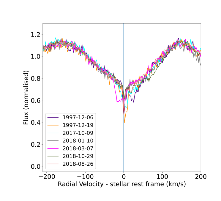
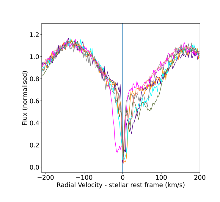
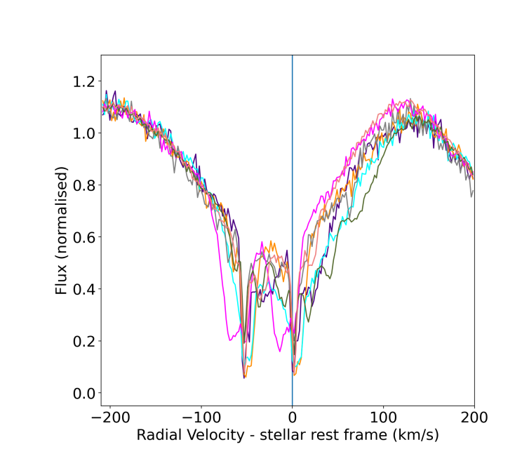
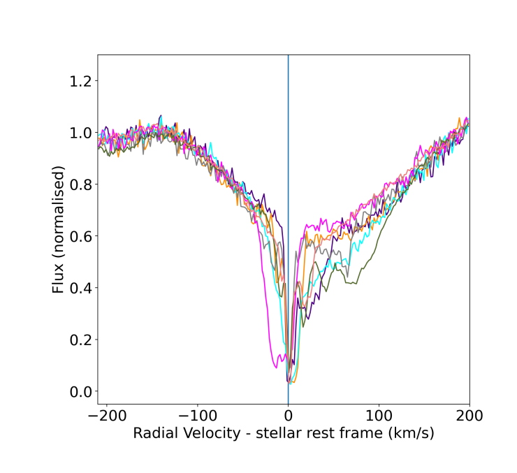
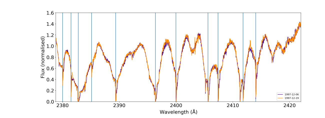
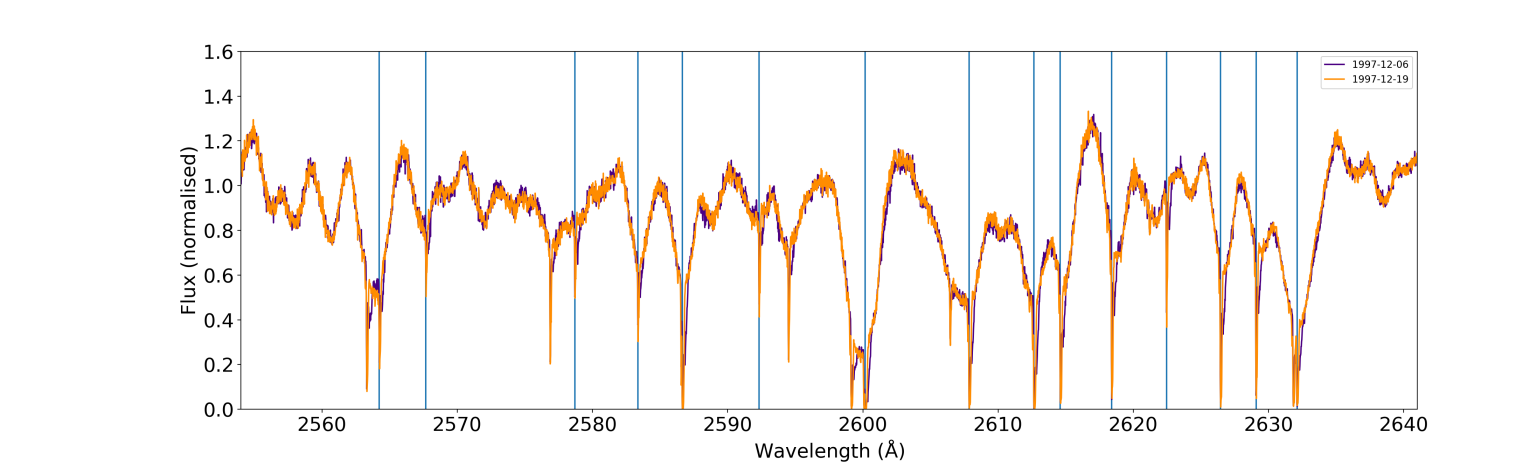
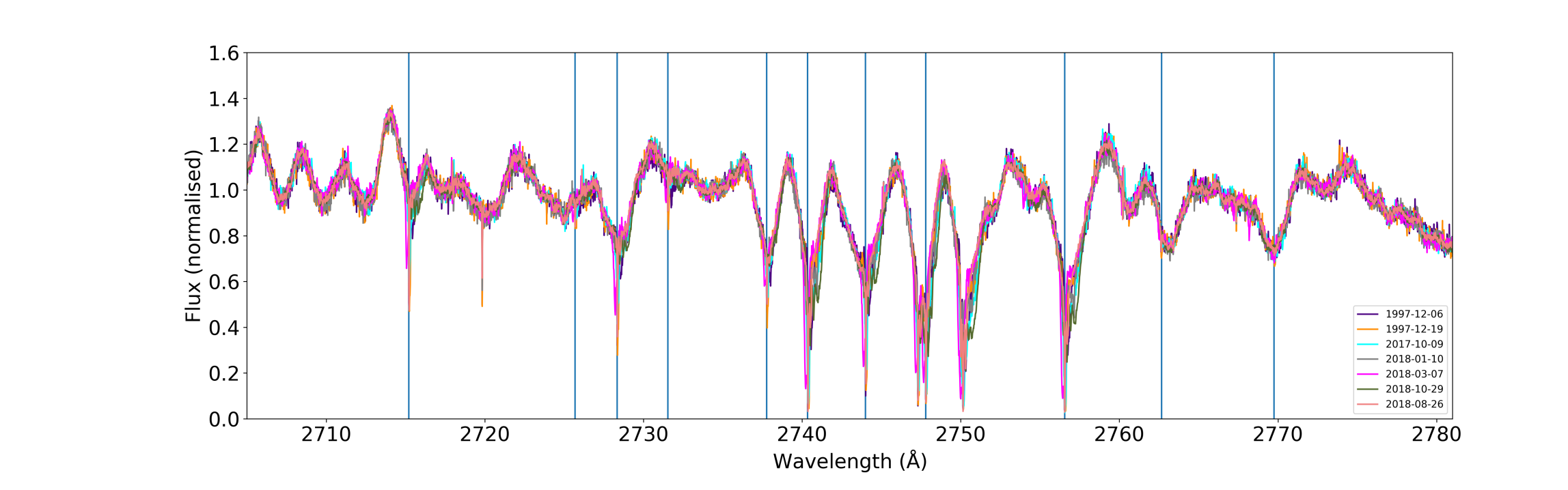
All these spectra cover the ionised iron (Fe ii) line series between 2715 and 2769 , rising from the 3d6(5D)4s - a4D metastable levels, in which cometary transits are easily detected (see sect. 2.3). In addition, the two 1997 observations (programme # 7512) also cover the Fe ii line series at 2400 and 2600 , which rise from a wide range of energy levels.
2.2 Data analysis
Each of the STIS/E230H spectra covers a bandwidth of about 270 Å wide, with a set of 24 to 40 orders of about 12 Å wide, partially overlapping. For each exposure, the fluxes of all the orders have been combined into a single spectrum and resampled on a common wavelength table with a resolution of 18 mÅ. The wavelengths were also corrected for the heliocentric radial velocity of Pic, +20 km/s (Gontcharov, 2007), so that they correspond to the Pic reference frame.
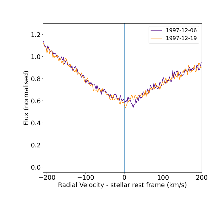
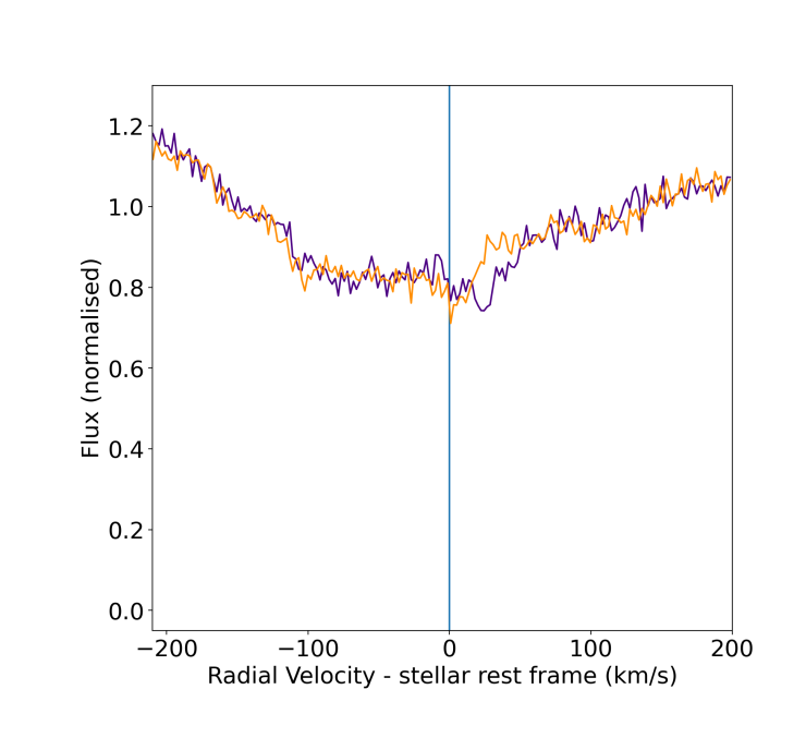
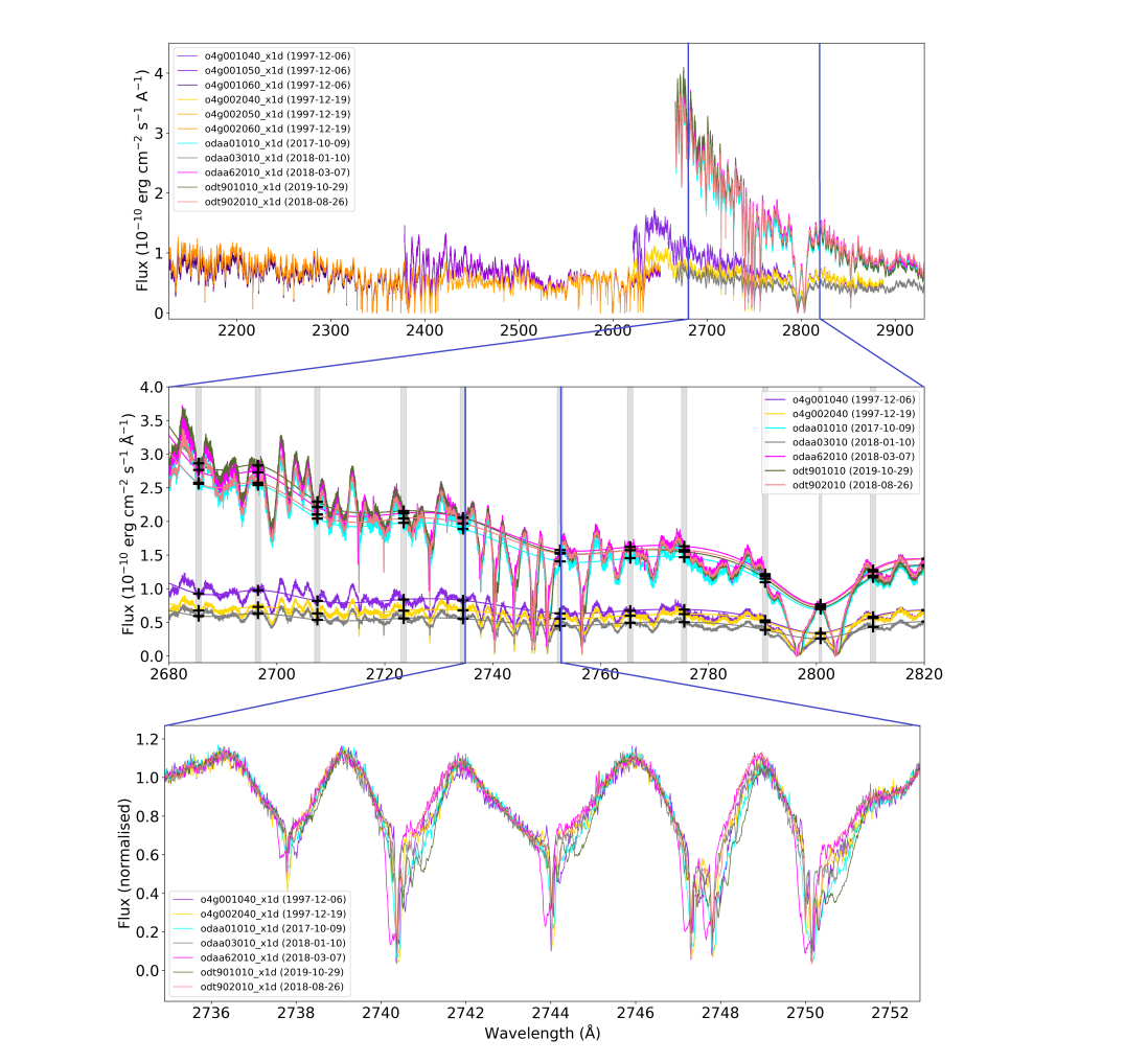
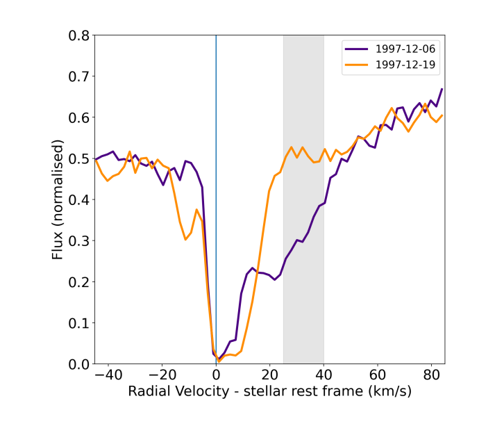
In a second step, to correct for variation of the flux calibration from one epoch to another, we renormalised the measured flux to a common flux level, independent of exocomet activity. For that, we selected a set of 65 1-wide regions free of any variations (i.e. mostly outside spectral lines) separated by 10 to 20 Å. By measuring their flux on these different regions, we obtained, for each spectrum, a set of reference points of the form . The reference points of each spectrum were then fitted by cubic splines, and each spectrum was divided by its corresponding spline. This flux normalisation allowed us to obtain data that can be easily compared, unveiling variable absorption features around many lines (Fig. 1).
Finally, as no significant spectral variation was observed within each set of three exposures taken on December 6 and December 19, 1997 (both times within a single HST orbit of minutes), these sets of exposures were merged together, yielding a single spectrum from 2128 Å to 2888 Å for each of the two epochs. For the 2017-2018 observations, no such merging was necessary, as only one exposure was used for each visit. As a result, we ended up with seven normalised spectra: two spectra covering the 2128 Å to 2888 Å wavelength range taken 13 days apart in 1997, and five spectra covering the 2665 Å to 2931 Å wavelength range taken at five different epochs in 2017-2018.
2.3 Detected Fe ii lines
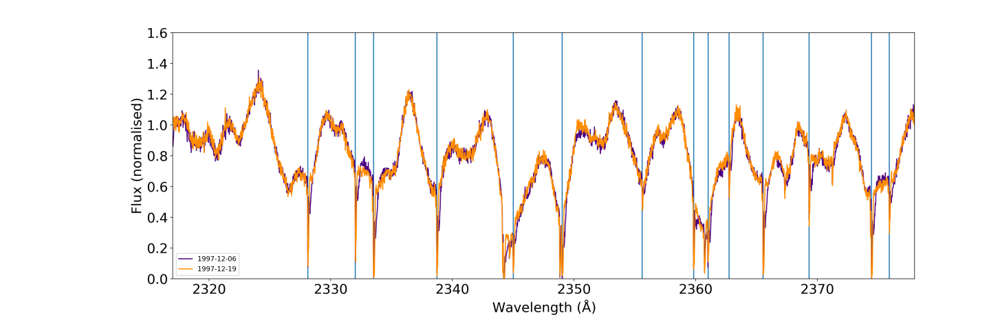
Dozens of Fe ii lines are detected in the seven analysed spectra, with deep absorption originating both from the circumstellar disc (stable) and from transiting evaporating comets (variable). These exocomet signatures are detected in three Fe ii main series: a first one near 2750 , where the high number of different visits (7) allows for distinguishing the variable absorptions from the stable stellar spectrum fairly easily (Fig. 14), as well as two other groups near 2400 and 2600 , only covered by the two 1997 observations (Fig. 15). In addition, a few lines arising from highly excited levels also showed fainter variable absorptions, as seen in Fig. 16. The complete list of lines used in the following sections is presented in Tables 3 (for the strongest lines) and 4 (for the lines arising from high energy levels).
2.4 Reconstruction of the comet-free spectrum
In order to quantify the variable features observed in these many Fe ii lines, particularly in the series at 2750 , one must first compute a stellar reference spectrum without cometary absorption. To do so, we proceeded in two main steps:
-
•
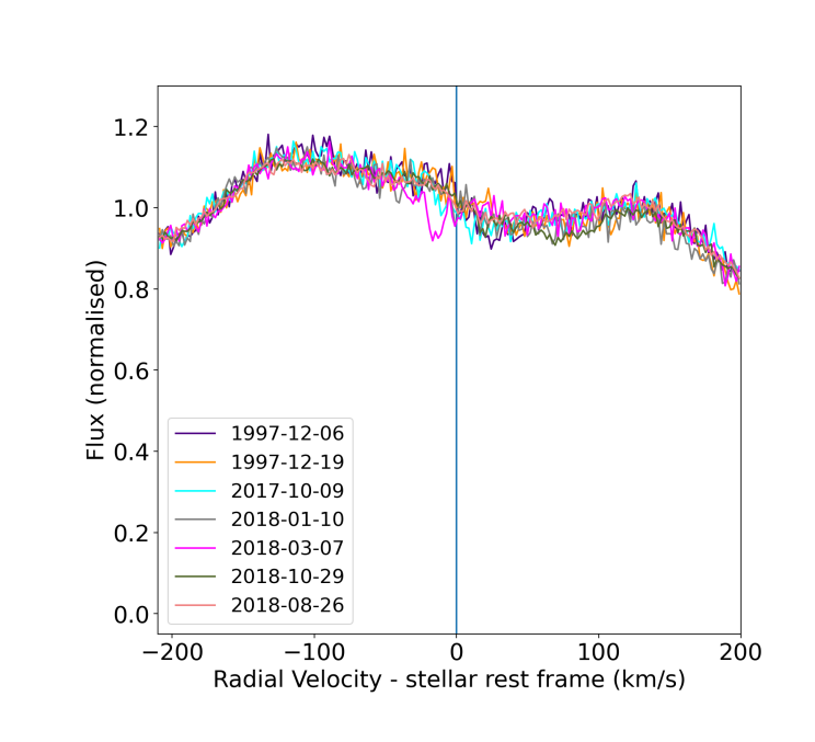
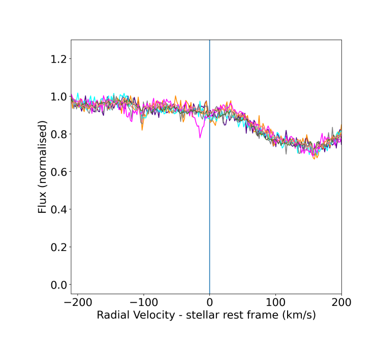
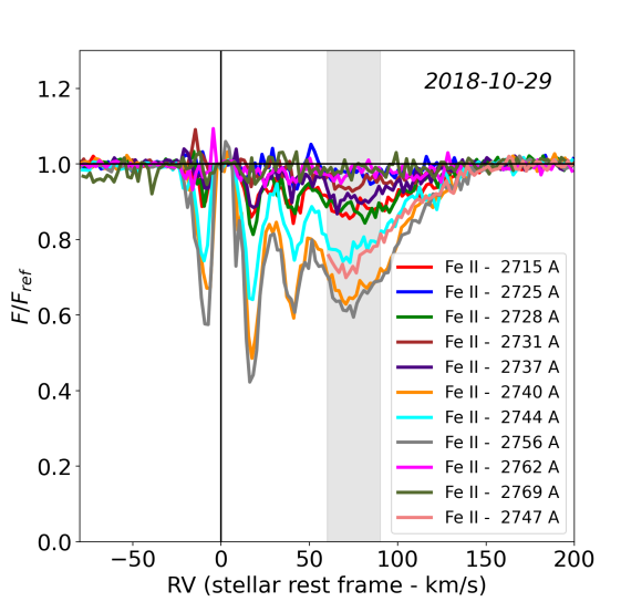
First, we used the 2750 Fe ii lines to identify, for each spectrum, the radial velocity domains where cometary absorption occurs, assuming it always occurs at the same radial velocities from one line to another (this assumption is in fact easily verified; see Sect. 2.5). This identification is made possible by the large number of spectra at these wavelengths, which allows us to easily distinguish, for each observation, the spectral domains where it is affected by cometary absorption and the spectral domains where it is not (see, e.g. Fig. 14). More quantitatively, for each radial velocity , we considered that a given spectrum is affected by cometary absorption when its flux at the velocity in the 2740 and 2756 lines (those are the strongest lines of the 2750 series) is at least 5 % below the brightest observation. The list of the radial velocity domains where cometary absorptions are detected is given for each observation in Table 2: we note that, for each radial velocity, there is always at least one comet-free observation, thanks to the rather high number of independent visits.
Table 2: List of radial velocity ranges where cometary absorption is detected, for each observation. Date of observation RV ranges with cometary absorption (km/s) a 1997-12-06 [-4; +200] 1997-12-19 [-17; +19 ], [+50; +150] 2017-10-09 [-35; +120] 2018-01-10 [-70; 0], [+19; +150] 2018-03-07 [-40; +13] 2018-10-29 [-30; -4], [+8; +140 ] 2018-12-15 [-40; +50] -
a
The radial velocities are given in Pic rest frame.
-
a
-
•
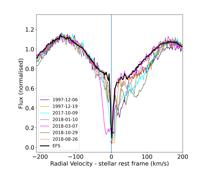
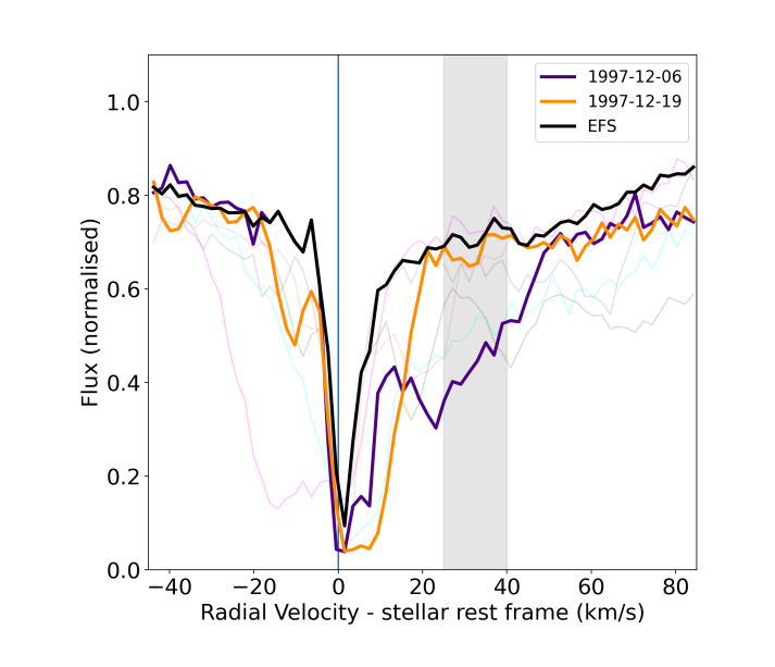
Second, for each wavelength pixel, we used the list of the radial velocity domains where comets are detected in each spectrum (Table 2), and the list of all the Fe ii lines (Tables 3 and 4), to determine the set of observations that can be considered comet-free at this particular wavelength. We then averaged all these un-absorbed spectra (free of cometary absorption) to obtain the reference spectrum of Pic. For instance, for the line at 2740 Å (Fig. 2), the comet-free spectrum between +50 and +120 km/s is obtained by averaging the 2018-03-07 and 2018-12-15 observations.
We note in Fig. 2 that it is not completely clear weather the spectrum obtained through this calculation is indeed the Pic comet-free spectrum. For instance, shallow comets may have been missed in our identification, leading us to underestimate the reference spectrum by a small fraction (typically a few percent). On the other hand, the reference spectrum might be slightly overestimated near + 30 km/s because of higher flux at the corresponding wavelengths in the March 7, 2018 observation (see Fig. 2, pink line). However, the impact of these biases on the calculation of the comet-free spectrum is much smaller than the typical signature of a Pic exocomet on its host star spectrum (which can cause absorption depths as high as 50 %). The conclusions presented in this paper are thus not significantly affected by such systematic errors.
It should also be noted that this comet-free spectrum can still contain interstellar and circumstellar absorption. However, because these absorptions are stable, they do not impact the measurement of cometary absorption depth. They can thus be included in the stellar reference spectrum, as if they had a stellar origin.
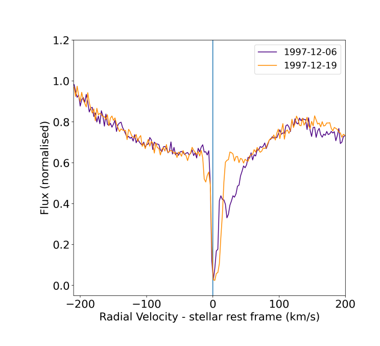
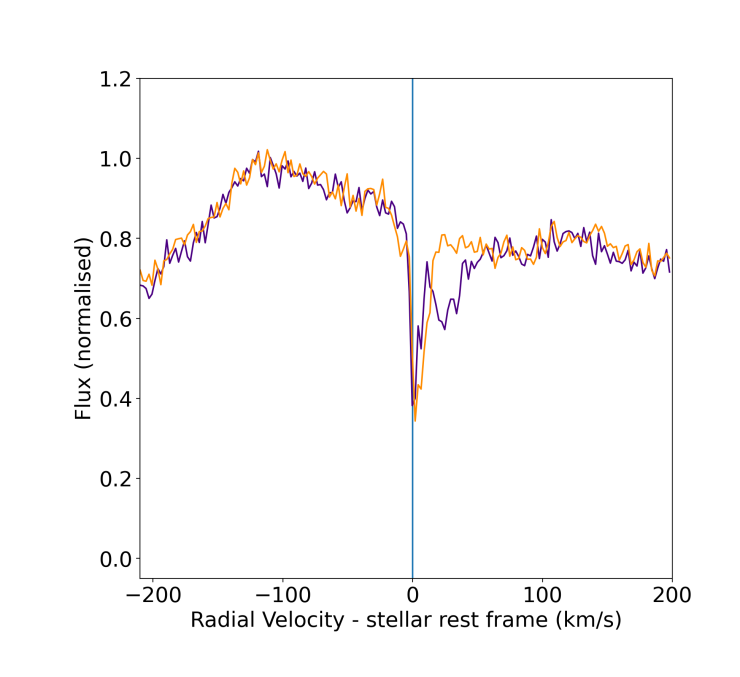
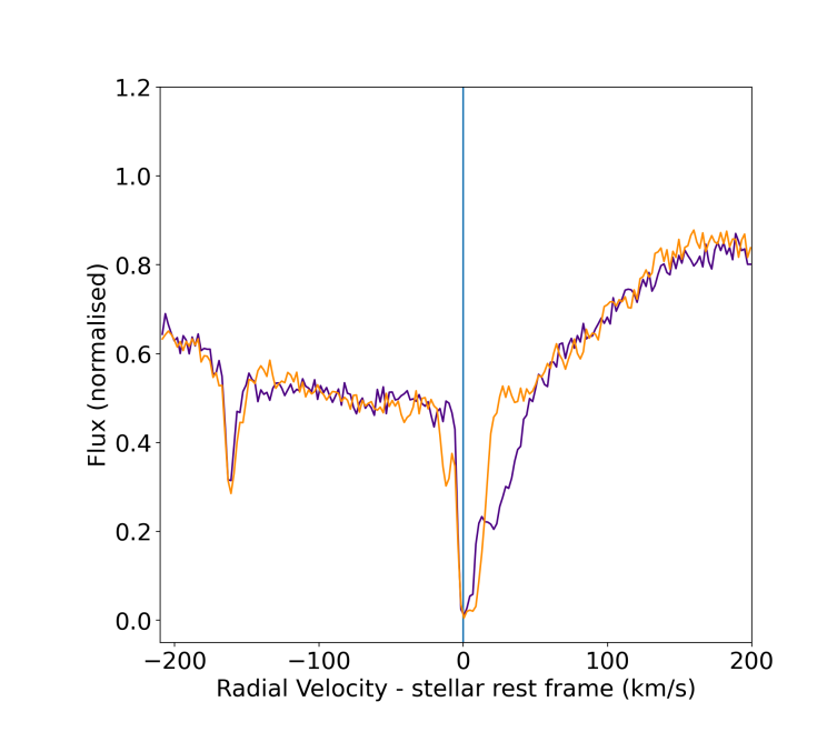
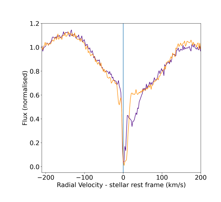
2.5 Cometary absorption
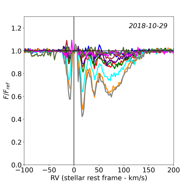
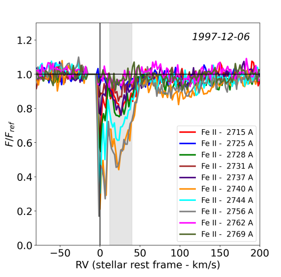
Cometary absorption spectra are obtained by dividing each individual observation by the comet-free spectrum previously calculated. This provides, for each observation, the absorption spectrum of the transiting gas: this spectrum is equal to one in spectral ranges where the transiting comets are transparent, and tends to zero in the presence of an optically thick tail. These spectra show the striking correlation between the absorption features observed in various Fe ii lines, within the same observations. For example, Fig. 3 shows, for two separate visits, the superposition of their cometary absorption spectra around ten different Fe ii lines, clearly revealing the transit of numerous comets within each of the observations.
The analysis developed in the next sections is focussed on the ’absorption depth’ and ’average absorption depth’ of exocomets. These two quantities are defined as follows:
-
•
For a given line (, ) (where and denote the lower and upper levels of the transition, respectively) and some given radial velocity , the absorption depth of exocomets is defined as the fraction of the stellar flux absorbed by exocomets at the velocity in the line (, ) in a given observation. If we denote the cometary absorption spectrum computed previously by this absorption depth writes as
The absorption depths thus range from zero in the absence of transiting comet to one when an optically thick cloud eclipses 100% of the stellar surface. The error bars on the measured absorption depths are estimated by accumulating all the errors on each of the used HST spectra as tabulated by the calstis pipeline.
-
•
Then, to improve the signal-to-noise ratio (S/N) of our absorption measurements, the exocomet absorption depth can be averaged over an extended radial velocity range. For some radial velocities and some line , we thus introduce the mean absorption depth of exocomets, which is defined as the average value of over the RV domain :

3 Model description
3.1 Principle
In order to interpret the absorption features due to the transit of exocomets, we used a modified version of the cometary model that Kiefer et al. (2014b) introduced to analyse the absorptions in the 3900 Ca ii doublet of Pic. The gist of the model is to assume that the absorption depth (relative to the comet-free spectrum; see Sect. 2.5) observed at a radial velocity in a set of lines from a given chemical species is produced by a gaseous cloud of homogeneous column density, covering a fraction of the stellar disc surface. Under these assumptions, the absorption depth of a transiting comet is given, for any of the considered lines, by
with and being the lower and upper levels of the line (noted below ) and the optical thickness of the cometary cloud, which can be expressed as
where is the Einstein coefficient for photon absorption of the considered line, Nl the column density of the lower energy level of the transition and the radial velocity distribution within the cloud (). The Einstein coefficient is linked to the oscillator strength of the transition through
| (1) |
Then, if we average the cometary absorption depth over a radial velocity range [] where is assumed to be constant, we can re-write and as
where is the mean absorption depth in the radial velocity range [; ] in the considered line, relative to the comet-free spectrum (see Sect. 2.5), the mean size of the comet in this range, and N the column density of the considered species at the lower energy level of the transition with a radial velocity between and . This set of equations is valid for any line of the considered chemical species.
3.2 Two-parameter model
Equation (LABEL:equation_modele_général) can be used to fit the mean absorption depth of a comet in a set of lines rising from the same excitation level of a given species, probing its column density . However, in the case where absorption features are detected in various lines rising from several excitation levels, one must find a way to link the various of these levels in order to combine the information they provide and infer the global properties of the transiting comet.
The easiest way of doing this is to consider the case where the excitation levels are sufficiently close in energy to be populated according to their multiplicity, that is, . In particular, this hypothesis is valid at local thermodynamic equilibrium (LTE), when, for any pair of transition and , we have
where T is the temperature of the absorbing medium, , the lower level energies of the lines, and the Boltzmann constant.
In these conditions, we thus have (Eqs. (1) and (LABEL:equation_modele_général)). We can therefore introduce a parameter defined such as
where is an arbitrary wavelength. For practicality, in the following is chosen to be equal to the wavelength of the 2756 Fe ii line; however, this choice has no impact on the results as it can be seen as a normalisation unit for . Indeed, the parameter is a unitless quantity common to all the studied lines and close to the optical thickness when . is thus related to the column densities of the excitation levels giving rise to the observed lines through
Using Eq. (2), we thus obtain the resulting curve of growth equation relating to the mean absorption depth within a radial velocity range to the line strength:
| (2) |
We note here that , and depend on the radial velocity range where the absorption depths are measured. Thus, to use this model, one must first measure the mean absorption depths of a transiting comet in a set of lines with various absorption strengths (), in a fixed RV range, and then fit the curve of growth model to these measured absorptions using Eq. (2) in order to estimate the values of and that best fit the observations. The column densities of the studied excitation levels can be then derived from the value of using
This two-parameter model was used by Kiefer et al. (2014b) to determine , the typical size of the gaseous clouds, of almost 500 comets transiting Pic detected in the Ca ii doublet. However, in this case, the model was fit to only two absorption measurements (one for each line of the doublet); it was thus not possible to check that it was realistic. To show that the model is correct and that the measured absorptions really follow a curve of growth as given by Eq. (2), a larger number of lines with various oscillator strengths is needed. The many () Fe ii lines observed with STIS, which show clear cometary absorptions, are thus a very useful tool to test the curve of growth model (Sect. 4).
3.3 Thermodynamical equilibrium: A three-parameter model
In the case where the cometary absorptions are detected in lines arising from a large variety of excitation levels, the hypothesis may no longer be a good approximation. For instance, very excited levels may be under-populated compared to ground states. To model the relative abundances of the considered energy levels, another possibility is to assume that the absorbing cloud is at LTE, with a typical temperature of (where, again, [; ] is the considered radial velocity range). This implies
We note that this new assumption requires a sufficiently high electronic density to impose a collisional regime. At LTE, Eqs. (1) and (LABEL:equation_modele_général) now yield . This allows the introduction of a new parameter , linking the optical thickness to the line strength through
Once again, is a unitless parameter common to all studied lines, close to the optical thickness when 1, and which depends on the radial velocity range where the mean absorption depths are measured. Thanks to Eqs. (1) and (LABEL:equation_modele_général), it can be linked to the abundance of the considered excitation levels within , through:
Summing the previous equation over all the excitation levels of the considered species, one then deduces
where reflects the total column density of the species with radial velocity between and , and Z is defined by
We therefore end up with a three-parameter curve of growth model that links the mean absorption depths of a transiting cloud in a set of lines of a given species, measured on a fixed radial velocity range, to the mean size (), temperature (), and total column density (via the parameter) of the absorbing cloud, through
| (3) |
where, again, , , and depend on the radial velocity range where the mean absorption depths are measured. Once these three quantities have been constrained by a curve of growth model fit to the measured absorption depths, one can estimate the total column density of the studied species through
We note that this model is valid under the assumption of column density and temperature homogeneity of the absorbing gas over the considered radial velocity range. This hypothesis can be checked by fitting the curve of growth model (Eq. (3)) to the cometary absorptions, as done in Sect. 5. If the measured absorptions do indeed follow the model, then the fitted parameters (, , ) may represent valuable estimates of the typical properties of the transiting cometary cloud.
Finally, the two-parameter model described in Sect. 3.2 can be seen as a simplified case of the three-parameter model, where the temperature is taken to be much higher than the energy difference between the excitation level of the considered lines. Indeed, in such a case, is constant over the set of lines, thus yielding (Sect. 3.2). The parameter introduced in the previous section is then linked to through
where this equation holds for any of the considered energy level . In particular, this is the case when there is only a single excitation level for the observed set of lines, as for the Ca ii doublet at 3933 and 3369 Å.
4 Validation of the two-parameter model
In order to validate our different models, we focus on two separate events in the following. The first one is the transit that occurred on December 6, 1997, between +12 and +40 km/s (see Fig. 3). Its main advantage is that it was observed in a great variety of Fe ii lines (in particular, in the three main series at 2400, 2600, and 2750 ), which will be useful for validating the three-parameter model in the next section. The second transit is the one from the October 29, 2018 observation, between +50 and +150 km/s (see Fig. 3), which benefits from a very good S/N (about 100) due to the long duration of the exposure. Another advantage of these transits is their high radial velocities, making them unaffected by the circumstellar absorption near 0 km/s (which reduces the S/N and may show long-term variability, Kiefer et al. (2019)).
The two-parameter curve of growth model was validated using the Fe ii line series around between 2715 and 2769 arising from the a4D Fe ii term. Indeed, the four levels that make up this state share close excitation energies (corresponding to temperature between 11448 and 12771 ; see Tables 3 and 5), allowing us to make the hypothesis - which we verify below - that their relative abundances are proportional to their multiplicity.
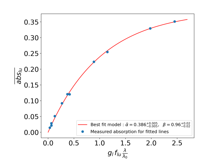
Figure 4 shows a first example of a curve of growth fit (lower panel) for the redshifted comet observed in the December 6, 1997 data (upper panel). The mean absorption depths were measured in the [+12; +40] km/s radial velocity range, corresponding to the main domain where this comet is visible. These absorption measurements were then fit with the two-parameter curve of growth model, using a Markov chain Monte Carlo (MCMC) algorithm. Remarkably, the ten absorption measurements follow the two-parameter curve of growth model very well (reduced of 2.7), constraining the average size of the transiting comet to of the stellar surface.
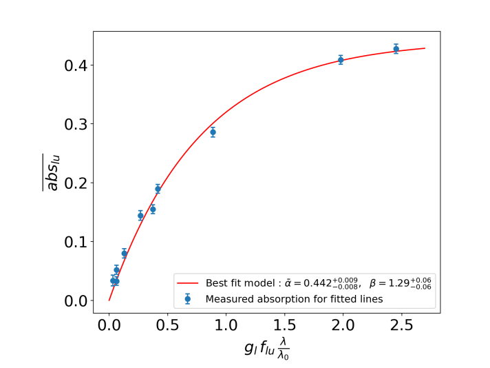
Another example is given in Fig. 5 for the October 29, 2018 event, where the comet mean absorption depths are measured from +60 to +90 km/s (the radial velocity range where it is the strongest). For this comet, we also took into account the reddest line of the 2747 doublet (see Fig. 14). Again, the two-parameter model fits the 11 measured absorptions strikingly well (reduced of 1.9), and constrains the mean size of the comet to of the stellar disc (within this velocity range).
These two examples clearly show that the variable features observed in the Fe ii lines of Pic are explained well by the transit of homogeneous cometary clouds, covering large but limited fractions of the stellar disc, and in which the sub-levels of the a4D Fe ii term have relative abundances proportional to their multiplicity. This remarkable agreement between the measured absorptions and the two-parameter curve of growth model also validates the results of Kiefer et al. (2014b), who applied this model to the Ca ii doublet at 3900 to identify two families of exocomets in the Pic system.
In addition, if we assume that the transiting cloud is at LTE (which is probably a reasonable assumption, as shown in Sect. 5) and use the three-parameter model to fit the measured absorption depths (Eq. (3)), we can put lower limits on the gas temperature around for the December 6, 1997 comet, and for the October 29, 2018 comet, at a 95 % confidence level. This is due to the fact that the lines rising from the most excited levels of the a4D term ( ; see Table 5) do not show significantly lower absorption than the lines rising from the less excited levels ( ): the gas temperature must thus be well above the energy difference between all these states, that is, .
Lower limits (with a confidence) can also be set on the total Fe ii column density within the transiting clouds in the considered radial velocity ranges, at about (December 6, 1997) and (October 29, 2018), which would be reached for temperatures between and .
The very high temperatures hinted in the tails of these two comets (similar to or above the effective temperature of Pic) are consistent with the results that were obtained by Mouillet & Lagrange (1995) using Ca ii triplet lines arising from the 3D metastable level. This shows that such objects are experiencing very strong compression, which releases heat (see Beust & Tagger, 1993). This compression is also likely responsible for the production of the observed highly ionised species such as Al iii or Si iv.
5 Validation of the three-parameter model
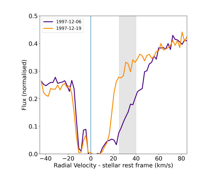
5.1 Temperature measurement
The analysis in Sect. 4 yielded striking results about the shape and thermodynamical conditions in the transiting cometary clouds of Pic. However, only lower limits could be set on their temperature and column density, as the energy difference between the different sub-levels of the Fe ii a4D term (which gives rise the line series at 2750 ; see Tables 3 and 5) was too low to probe the energy distribution of Fe+. Luckily, the two 1997 observations also cover the 2300-2600 wavelength range, where a large number of Fe ii lines rising from a wider range of excitation levels are present (see Table 3). In addition to the ten previously studied lines, we thus included in our analysis 31 new lines with wavelengths between 2328 Å and 2629 Å, and with lower level energies from 0 to 12700 K (0 - 8000 ). For the lines arising from low energy levels (), we limited ourselves to the ones with average values of the absorbing strength (), avoiding both the weakest transitions (), for which the S/N on the absorption depth is weak, and the strongest ones (), which showed abnormally strong absorption depths (see the discussion in Sect. 6). However, wavelengths below 2600 Å are only covered by the two 1997 observations. This prevents us from building a proper reference spectrum at these wavelength (as we did in Sect. 2.4 for the 2750 lines), as there are wide ranges of radial velocities where both 1997 spectra seem affected by comets (see Table 2) and where, therefore, it is impossible to recover the unnoculted stellar flux. To exploit these lines and test our three-parameter curve of growth model, we thus chose to focus on the redshifted comet observed on December 6, 1997 (Fig. 4) and limited our study to the [+25; +40] km/s radial velocity range. Indeed, in this narrower velocity range, the other 1997 observation taken 13 days later seems to be little affected by comets (Fig. 6), providing a sufficiently reliable estimate of the unnoculted Pic spectrum and enabling us to retrieve the absorption depth of the December 6, 1997 comet in the Fe ii lines between 2300 Å and 2600 . Here, for the sake of consistency, we also used the same December 19, 1997 observation as a reference spectrum for the 2750 lines, despite the fact that other observations are available. This choice, however, has very little incidence on our measurements; the results would be very similar if we had used the ’comet-free’ spectrum as a reference for these lines, as we did in the previous section.
(), showing the only two available spectra for this line.
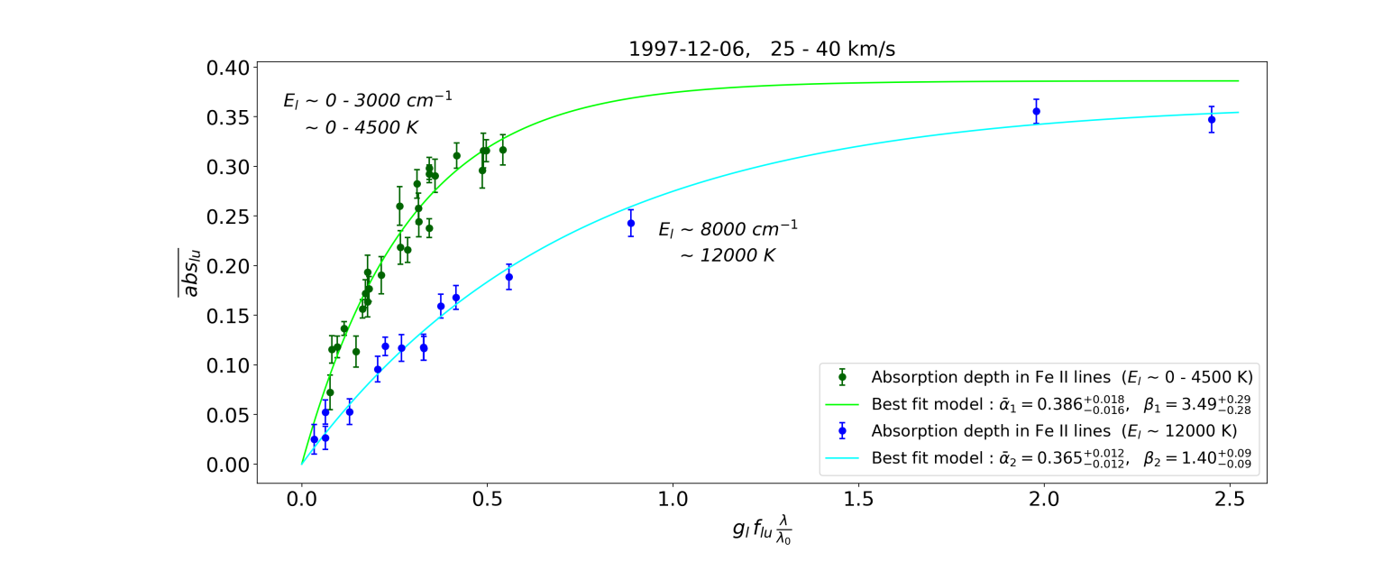
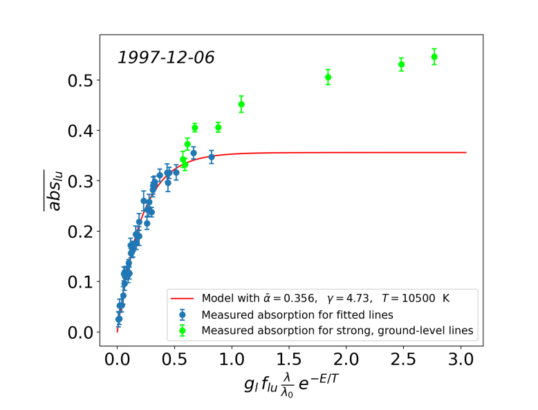
First, we started by separately fitting the mean absorption depths of the December 6, 1997 comet in the lines rising from low-energy levels ( ; i.e. ) and higher energy levels ( ), using the two-parameters curve of growth model tested above. The results are provided in Fig. 7; we note that the two sets of lines constrain the size of the absorbing cloud to very close values ( % for the ground levels lines, % for the metastable lines), hinting that the absorptions occurring in both sets are produced by the same gaseous component. We note, however, that the lines rising from ground Fe ii levels are more easily saturated than the lines rising from excited levels ( for the first, for the last): this reveals the significant under-population of the excited levels due to a finite temperature in the absorbing medium.
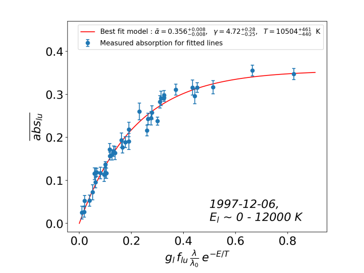
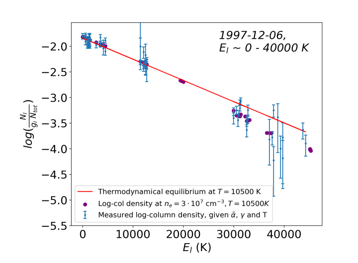
We then fitted the 41 Fe ii lines all together, with the addition of a new free parameter: the temperature. Despite the very high number of measurements, three free parameters seem to be enough to fit the data all together. Indeed, our curve of growth model matches the measured absorption depths remarkably well (), allowing us to constrain the temperature of the absorbing medium at and its average size at of the stellar surface (Fig. 8). The total Fe ii column density in the studied radial velocity range (i.e. between +25 and +40 km/s) was thus estimated to be .
In order to better visualise the temperature of the absorbing gas, it is also possible to build an excitation diagram of Fe+ within the comet. Indeed, the model Eq. (3) can be re-written as
yielding
| (4) |
The slope of expressed as a function of is therefore inversely proportional to the temperature . On the other hand, knowing , which characterises the typical size of the absorbing cloud independently of the line considered, we can derive an estimate of from each absorption measurement in any spectral line arising from the energy level to within one additive constant depending on , and . Therefore, the temperature of the transiting cloud can be directly estimated through the variation of (the relative abundance of the various Fe+ excitation levels, normalised by their multiplicity) as a function of . This is illustrated in Fig. 9, where we can clearly see that the a4D energy levels () are significantly under-populated when compared to the ground levels due to the finite temperature () within the transiting gas.
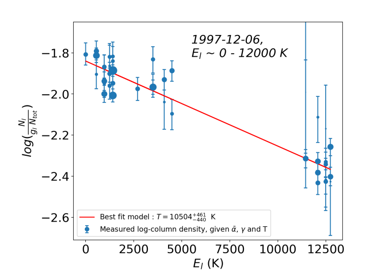
. The y-axis represents the log-relative abundance of the studied Fe ii energy levels, within an additive constant (see Eq. (4)), while the x-axis indicates the energy of these levels. Each point thus represents an abundance estimate of an energy level , based on the measurement of the absorption depth in a given line . As some lines rise from the same energy level, some of these levels benefit from several independent abundance measurements. The marker sizes are inversely proportional to the vertical uncertainties.
We can finally extrapolate this temperature to the whole velocity range of the December 6, 1997 comet (i.e. between +12 and + 40 km/s) in order to estimate its total column density (which was found in Sect. 4 to be greater than ). Indeed, fitting the 2750 lines’ absorption depths measured in this velocity range again with a Gaussian prior on the temperature of , one can deduce a total Fe ii column density in the transiting gas of . Given the relative size of the comet ( of Pic surface, Fig. 4), the radius of Pic () and the mass of an iron atom (), we can convert this column density into a mass of , which is equivalent to of pure iron (density ). This tremendous mass shows the intense evaporation occurring at the surface of these cometary nuclei, hinting that they have very short lifetimes and may not survive to even a single periastron passage. This remark therefore indicates that a large fraction of the comets observed to transit Pic may originate from a recent break-up of a former massive body, as was suggested in Kiefer et al. (2014b) for the D family of Pic comets.
5.2 The electronic density
Until now, our study was focussed on Fe ii lines arising from energy levels below 12 000 , assuming that the transiting cloud is at LTE. Using the ChiantiPy Python module (Landi et al., 2012), which allows us to compute the energy distribution of many ions at given temperature and electronic density (), it can be shown that this hypothesis is easily verified, roughly requiring . This allowed for an estimate of the absorbing gas temperature, assuming that the excitation temperature of the low-energy Fe ii levels (deduced from the excitation diagram, Fig. 9) is equal to the kinetic temperature.
In addition to the lines studied in Sects. 4 and 5, cometary absorption is also detected in a few lines arising from highly excited Fe ii levels (from 30 000 to 40 000 ; see Table 4 and Fig. 16) at wavelengths between 2400 and 2900 . A key feature of these lines is that their lower levels require much higher electronic densities to be populated at LTE, around (ChiantiPy Landi et al., 2012); at low densities, they tend to be less populated than at LTE. Thus, this set of lines can be used as a probe of the electronic density within the transiting cometary tails. To do so, we started by measuring the mean absorption depths of the December 6, 1997 comet in the [+25; +40] km/s range for 26 high-energy Fe ii lines. Then, given the cometary cloud properties measured in Sect. 5.1 ( , , ), we used these absorption measurements to extract the relative abundances of the energy levels corresponding to those lines (Eq. (4)). These abundance estimates rely on the fact that the second equality in Eq. (4) remains valid for energy levels that are not populated at LTE, as long as most of the absorbing gas follows a Boltzmann distribution:
Then, we compared these relative abundances to the values predicted by LTE at the measured temperature () by building the complete excitation diagram of Fe ii within the cometary tail (Fig. 10). This diagram clearly shows that high-energy ( ) Fe ii levels are under-populated compared to LTE, hinting that the electronic density is not high enough to impose a Boltzmann distribution.
Finally, in order to quantify the typical electronic density within the cometary cloud, we compared the energy distribution of Fe ii measured in our spectra to the theoretical energy distribution for various electronic densities, obtained with ChiantiPy (to compute the distribution, a temperature of was used, as measured in Sect. 5.1). Although it is difficult to give a precise estimate, the excitation diagram of Fe ii given in Fig. 10 seems to indicate an electronic density in the [2-4] range. These results are consistent with the work of Mouillet & Lagrange (1995), where a minimum electronic density of in a transiting comet was inferred from its absorption in the Ca ii triplet.
6 Discussion
6.1 Deviation from the curve of growth model
The analysis of the exocomet transit signature in the December 6, 1997 observation shows that the transiting gas in the [+12; +40] km/s range is described well by an homogeneous cloud covering, on average, 44% of the stellar surface, with a total Fe ii column density of , a temperature of (Sect. 5.1), and an electronic density of approximately (Sect. 5.2). These results were obtained by using most of the well-detected Fe ii lines in the 2300 - 2800 wavelength domain. However, we note that for a few very strong lines ( ) rising from low energy levels (), the measured absorption depth seems to deviate from the curve of growth model. For instance, the mean absorption depth of the December 6, 1997 comet in the [+25; +40] km/s range exceeds 50% for the lines at 2383 (), 2396 () and 2600 (, see Fig. 11), which is well above the measured size of the cometary cloud () in this radial velocity domain.
This discrepancy between the curve of growth model fitted in Sect. 5.1, which matches the measured absorption depths on the ”weak” Fe ii lines () strikingly well, and the absorption measured in the strongest ones () can be revealed by plotting the curve of growth model with all the absorption measurements (Fig. 12). We see that while the cometary absorption depths in the weakest Fe ii lines (blue dots) saturate towards , the absorption in strong, ground-level Fe ii lines (green dots) keeps increasing slowly as the line strength () increases. This shows that the complexity of the transiting object is probably underestimated by our model. For instance, the absorption measurements might be better explained by the transit of at least two gaseous components: a dense one, which quickly saturates towards a 36 % absorption depth as the line strength increases, and a thinner one, saturating more slowly, explaining why the absorption increases again by about when we reach the strongest lines.
Although our simple model allows for a fairly accurate characterisation of transiting comets, it thus fails to probe the complex structure that such objects probably have. Nevertheless, our study shows the tremendous potential of the many near ultraviolet Fe ii lines for investigating the properties of the transiting gaseous tails. This paves the way for the development of more sophisticated models, in order to interpret the variable features observed in the spectrum of several stars in even greater detail. Such models may allow us to probe the temperature and density distribution of the transiting clouds - which are probably not perfectly homogeneous, as revealed by the study of the December 6, 1997 comet - as well as the orbital dynamics of the evaporating nucleus. In particular, one key objective of forthcoming works will be to infer the radial velocity of the nucleus from the absorption profile of its tail.
These models will also have to take into account the inhomogeneous distribution of the stellar flux at a given wavelength on the stellar disc. Indeed, this distribution is affected by limb darkening, which reduced the luminosity of the edges of the stellar disc, and by the rapid rotation velocity of stars such as Pic (130 ), which shifts the local stellar lines. Strictly speaking, occulting a fraction of the stellar disc is thus not equivalent to reducing the stellar flux by a fraction at each wavelength. This subtlety, which was neglected in our study, might actually be useful to constrain the 2D distribution of transiting cometary tails, by probing the location of the stellar regions they occult.
6.2 Optical thickness profile
The curve of growth model developed in Sect. 3 to derive the physical properties of Pic exocomets uses the hypothesis that the optical thickness - characterised by the parameter - is constant over the radial velocity range where the cometary absorption depths are measured. In fact, it can be shown that, even if the optical thickness profile is not flat, the model still provides very good estimates of the size, temperature, and column density of the absorbing cloud. To check this, we generated artificial absorption spectra of transiting comets with known column densities, and with quickly varying optical thickness over radial velocity. We found that, as long as the optical thickness stays below unity, or does not vary by a large factor () over the studied radial velocity range, the curve of growth model provides very good estimates of the true physical parameters of the absorbing gas ().
To go further, we could also subdivide the radial velocity domain [, ] into elementary intervals and apply the curve of growth model to the absorption depths measured within every range [, ]. This would allow us to probe the radial velocity dependency of the size () and optical thickness () of the gaseous cometary cloud. Such an analysis could thus give a first insight into the geometry of a transiting gaseous tail, probing, in particular, how its size and optical thickness evolve as the gas is pushed away from the star by the radiation pressure. However, this analysis is far beyond the scope of the present work.
7 Conclusion
Using HST archival UV spectra of Pic, we detected variable absorptions in dozens of Fe ii lines, which are due to the transit of gaseous cometary tails. To better characterise the properties of these objects, we developed a simple model that describes the absorbing gas with a homogeneous cloud, covering a fraction of the stellar disc. This model matches the measured absorptions in most of the Fe ii lines remarkably well - with the exception of the strongest ones - showing that the variable features seen in the Pic spectrum are well interpreted by the transit of large (), dense (N) and hot () cometary gas tails. In the comet that transited in December 6, 1997, the population of the energy levels is consistent with LTE, which allows an estimate of the temperature within the gas tail of . Using Fe ii lines arising from highly excited electronic levels, we estimated the typical electronic density to be around a few in this cometary gas cloud. All the results obtained here are consistent with previous observational studies, notably with the quantitative estimates given by Lagrange et al. (1995), Mouillet & Lagrange (1995), and Kiefer et al. (2014b). They are, however, slightly different to the theoretical predictions of Beust & Tagger (1993), for which the formation of a shock front with very high temperature () and rather low density () is necessary to explain the presence of highly ionised species (such as Al iii) in the transiting cometary tails. Further work will be needed to better understand this discrepancy.
Our results also confirm the huge difference between Pic and solar comets; while the iron in Pic comets is mainly present as Fe+ (only very shallow cometary absorption is detected in Fe i lines; see Welsh & Montgomery (2016))), with column densities of the order of , solar comets contain mainly neutral iron, with much lower column densities (, Manfroid et al. (2021)). This is likely to be a consequence of the very short distance between Pic transiting comets and their star, which induces an intense sublimation of metal-rich material at the surface of the nuclei, while the tails of solar comets mainly result from the sublimation of volatile ices.
Finally, the curve of growth model appears to be an efficient tool to characterise the gaseous clouds surrounding transiting exocomets, detected through variable spectroscopic absorptions. The exocomet curve of growth is the analogue of the classical curve of growth used for interstellar clouds and stellar atmospheres. A fit to this curve provides quantitative estimates of the typical size of the absorbing cloud, and the column densities of the detected species. When several lines from various excitation energy levels are available, the temperature and possibly the electronic density can also be constrained. Further works using this new tool are already in progress.
Acknowledgements.
T.V., A.L., G.H. & A.V.-M acknowledge funding from the Centre National d’Études Spatiales (CNES).References
- Apai et al. (2015) Apai, D., Schneider, G., Grady, C. A., et al. 2015, ApJ, 800, 136
- Beust et al. (1990) Beust, H., Lagrange-Henri, A. M., Vidal-Madjar, A., & Ferlet, R. 1990, A&A, 236, 202
- Beust & Tagger (1993) Beust, H. & Tagger, M. 1993, Icarus, 106, 42
- Brandeker (2011) Brandeker, A. 2011, ApJ, 729, 122
- Brandeker et al. (2016) Brandeker, A., Cataldi, G., Olofsson, G., et al. 2016, A&A, 591, A27
- Ferlet et al. (1987) Ferlet, R., Hobbs, L. M., & Vidal-Madjar, A. 1987, A&A, 185, 267
- Gontcharov (2007) Gontcharov, G. A. 2007, VizieR Online Data Catalog, III/252
- Jolly et al. (1998) Jolly, A., McPhate, J. B., Lecavelier, A., et al. 1998, A&A, 329, 1028
- Kalas et al. (2000) Kalas, P., Larwood, J., Smith, B. A., & Schultz, A. 2000, ApJ, 530, L133
- Kennedy (2018) Kennedy, G. M. 2018, MNRAS, 479, 1997
- Kiefer et al. (2014a) Kiefer, F., Lecavelier des Etangs, A., Augereau, J. C., et al. 2014a, A&A, 561, L10
- Kiefer et al. (2014b) Kiefer, F., Lecavelier des Etangs, A., Boissier, J., et al. 2014b, Nature, 514, 462
- Kiefer et al. (2023) Kiefer, F., Van Grootel, V., Lecavelier des Etangs, A., et al. 2023, A&A, 671, A25
- Kiefer et al. (2019) Kiefer, F., Vidal-Madjar, A., Lecavelier des Etangs, A., et al. 2019, A&A, 621, A58
- Kramida et al. (2023) Kramida, A., Yu. Ralchenko, Reader, J., & and NIST ASD Team. 2023, NIST Atomic Spectra Database (ver. 5.11), [Online]. Available: https://physics.nist.gov/asd [2023, December 15]. National Institute of Standards and Technology, Gaithersburg, MD.
- Lacour et al. (2021) Lacour, S., Wang, J. J., Rodet, L., et al. 2021, arXiv e-prints, arXiv:2109.10671
- Lagrange et al. (2010) Lagrange, A. M., Bonnefoy, M., Chauvin, G., et al. 2010, Science, 329, 57
- Lagrange et al. (2019) Lagrange, A. M., Meunier, N., Rubini, P., et al. 2019, Nature Astronomy, 3, 1135
- Lagrange et al. (1995) Lagrange, A. M., Vidal-Madjar, A., Deleuil, M., et al. 1995, A&A, 296, 499
- Lagrange-Henri et al. (1989) Lagrange-Henri, A. M., Beust, H., Ferlet, R., & Vidal-Madjar, A. 1989, A&A, 215, L5
- Landi et al. (2012) Landi, E., Del Zanna, G., Young, P. R., Dere, K. P., & Mason, H. E. 2012, ApJ, 744, 99
- Lecavelier des Etangs et al. (2022) Lecavelier des Etangs, A., Cros, L., Hébrard, G., et al. 2022, Scientific Reports, 12, 5855
- Lecavelier des Etangs et al. (2001) Lecavelier des Etangs, A., Vidal-Madjar, A., Roberge, A., et al. 2001, Nature, 412, 706
- Manfroid et al. (2021) Manfroid, J., Hutsemékers, D., & Jehin, E. 2021, Nature, 593, 372
- Miles et al. (2016) Miles, B. E., Roberge, A., & Welsh, B. 2016, ApJ, 824, 126
- Miret-Roig et al. (2020) Miret-Roig, N., Galli, P. A. B., Brandner, W., et al. 2020, A&A, 642, A179
- Montgomery & Welsh (2012) Montgomery, S. L. & Welsh, B. Y. 2012, PASP, 124, 1042
- Mouillet & Lagrange (1995) Mouillet, D. & Lagrange, A. M. 1995, A&A, 297, 175
- Nowak et al. (2020) Nowak, M., Lacour, S., Lagrange, A. M., et al. 2020, A&A, 642, L2
- Pavlenko et al. (2022) Pavlenko, Y., Kulyk, I., Shubina, O., et al. 2022, A&A, 660, A49
- Rebollido et al. (2020) Rebollido, I., Eiroa, C., Montesinos, B., et al. 2020, A&A, 639, A11
- Roberge et al. (2000) Roberge, A., Feldman, P. D., Lagrange, A. M., et al. 2000, ApJ, 538, 904
- Roberge et al. (2006) Roberge, A., Feldman, P. D., Weinberger, A. J., Deleuil, M., & Bouret, J.-C. 2006, Nature, 441, 724
- Roberge et al. (2014) Roberge, A., Welsh, B. Y., Kamp, I., Weinberger, A. J., & Grady, C. A. 2014, ApJ, 796, L11
- Smith & Terrile (1984) Smith, B. A. & Terrile, R. J. 1984, Science, 226, 1421
- Snellen & Brown (2018) Snellen, I. A. G. & Brown, A. G. A. 2018, Nature Astronomy, 2, 883
- Strøm et al. (2020) Strøm, P. A., Bodewits, D., Knight, M. M., et al. 2020, PASP, 132, 101001
- Vidal-Madjar et al. (1986) Vidal-Madjar, A., Hobbs, L. M., Ferlet, R., Gry, C., & Albert, C. E. 1986, A&A, 167, 325
- Vidal-Madjar et al. (1994) Vidal-Madjar, A., Lagrange-Henri, A. M., Feldman, P. D., et al. 1994, A&A, 290, 245
- Welsh & Montgomery (2013) Welsh, B. Y. & Montgomery, S. 2013, PASP, 125, 759
- Welsh & Montgomery (2016) Welsh, B. Y. & Montgomery, S. 2016, PASP, 128, 064201
- Zieba et al. (2019) Zieba, S., Zwintz, K., Kenworthy, M. A., & Kennedy, G. M. 2019, A&A, 625, L13
Appendix A Line and energy level parameters
| b | b | |||
|---|---|---|---|---|
| () | ( | () | () | |
| 2328.11 | 668 | 960 | 6.60 | 0.215 |
| 2332.02 | 1873 | 2694 | 3.17 | 0.207 |
| 2333.51 | 385 | 554 | 13.1 | 0.643 |
| 2338.73 | 863 | 1242 | 11.3 | 0.371 |
| 2345.00 | 977 | 1406 | 9.27 | 0.306 |
| 2349.02 | 668 | 961 | 11.5 | 0.572 |
| 2355.61 | 2838 | 4084 | 2.67 | 0.089 |
| 2359.83 | 863 | 1242 | 5.00 | 0.251 |
| 2361.02 | 2430 | 3497 | 6.20 | 0.311 |
| 2362.74 | 2430 | 3497 | 1.41 | 0.095 |
| 2365.55 | 385 | 554 | 5.90 | 0.387 |
| 2369.32 | 2838 | 4084 | 6.06 | 0.204 |
| 2374.46 | 0 | 0 | 4.25 | 0.360 |
| 2375.92 | 3117 | 4486 | 9.80 | 0.166 |
| 2380.00 | 2430 | 3497 | 2.73 | 0.186 |
| 2381.49 | 668 | 961 | 3.10 | 0.211 |
| a 2382.76 | 0 | 0 | 31.3 | 3.203 |
| 2385.11 | 3117 | 4486 | 3.20 | 0.109 |
| a 2389.36 | 385 | 554 | 10.5 | 0.720 |
| a 2396.35 | 385 | 554 | 25.9 | 2.234 |
| a 2399.97 | 668 | 961 | 13.9 | 0.722 |
| a 2405.62 | 668 | 961 | 19.6 | 1.363 |
| 2407.39 | 863 | 1242 | 16.1 | 0.561 |
| 2411,80 | 977 | 1406 | 23.7 | 0.414 |
| 2414.04 | 977 | 1406 | 10.2 | 0.357 |
| 2564.24 | 8392 | 12076 | 15.1 | 0.597 |
| 2567.68 | 8680 | 12492 | 11.0 | 0.218 |
| 2578.69 | 8847 | 12731 | 12.0 | 0.240 |
| 2583.36 | 8680 | 12492 | 8.80 | 0.353 |
| a 2586.64 | 0 | 0 | 9.94 | 0.719 |
| 2592.31 | 8392 | 12076 | 5.70 | 0.345 |
| a 2600.17 | 0 | 0 | 23.5 | 2.386 |
| a 2607.87 | 668 | 961 | 17.3 | 0.707 |
| a 2612.65 | 385 | 554 | 12.0 | 0.984 |
| 2614.60 | 863 | 1241 | 21.2 | 0.435 |
| 2618.40 | 668 | 961 | 4.88 | 0.302 |
| 2622.45 | 977 | 1406 | 5.60 | 0.116 |
| 2626.45 | 385 | 554 | 3.52 | 0.365 |
| 2629.08 | 977 | 1406 | 8.74 | 0.363 |
| 2632.11 | 668 | 961 | 6.29 | 0.524 |
-
a
Lines discussed in Sect. 6 for the December 6, 1997 transiting comet.
-
b
The and values of the lines were found on the NIST database (Kramida et al. (2023)). The uncertainties are of the order of 10 %.
| () | ( | () | () | |
|---|---|---|---|---|
| 2715.22 | 7955 | 11448 | 5.70 | 0.379 |
| 2725.69 | 8392 | 12077 | 0.96 | 0.064 |
| 2728.35 | 8392 | 12077 | 9.38 | 0.420 |
| 2731.54 | 8680 | 12492 | 2.79 | 0.125 |
| 2737.78 | 8680 | 12492 | 12.2 | 0.275 |
| 2740.36 | 7955 | 11448 | 22.1 | 1.994 |
| 2744.01 | 8847 | 12732 | 19.7 | 0.891 |
| 2747.79 | 8392 | 12077 | 16.9 | 1.150 |
| 2756.55 | 7955 | 11448 | 21.5 | 2.454 |
| 2762.66 | 8847 | 12732 | 1.38 | 0.063 |
| 2769.75 | 8680 | 12492 | 0.48 | 0.033 |
-
•
Table 3. continued.
| a | a | |||
|---|---|---|---|---|
| () | ( | () | () | |
| 2424.88 | 22637 | 32578 | 22.1 | 2.34 |
| 2430.82 | 22810 | 32827 | 19.1 | 1.70 |
| 2445.26 | 20830 | 29977 | 27.8 | 2.00 |
| 2446.31 | 21812 | 31390 | 20.7 | 1.12 |
| 2471.42 | 22810 | 32827 | 15.4 | 0.85 |
| 2499.65 | 21581 | 31058 | 21.2 | 2.39 |
| 2512.52 | 21712 | 31246 | 23.0 | 2.18 |
| 2526.15 | 21251 | 30583 | 19.1 | 2.56 |
| 2527.05 | 20830 | 29977 | 24.7 | 1.42 |
| 2530.31 | 22637 | 32578 | 22.0 | 2.12 |
| 2530.32 | 21812 | 31390 | 20.2 | 0.78 |
| 2534.39 | 21430 | 30841 | 19.2 | 2.22 |
| 2535.18 | 21711 | 31245 | 18.3 | 1.41 |
| 2667.43 | 27620 | 39748 | 18.7 | 1.60 |
| 2685.55 | 30764 | 44273 | 15.7 | 1.70 |
| 2693.40 | 30388 | 43732 | 14.0 | 1.83 |
| 2704.79 | 27314 | 39308 | 13.8 | 1.21 |
| 2712.65 | 25428 | 36594 | 4.3 | 0.68 |
| 2717.02 | 27620 | 39748 | 11.5 | 0.77 |
| 2754.10 | 26352 | 37923 | 18.9 | 2.58 |
| 2768.32 | 26170 | 37662 | 15.8 | 2.55 |
| 2780.12 | 26352 | 37923 | 10.0 | 0.93 |
| 2784.51 | 26170 | 37662 | 10.6 | 1.23 |
| 2832.39 | 25787 | 37110 | 7.6 | 0.55 |
| 2841.48 | 26932 | 38758 | 7.6 | 0.37 |
| 2859.18 | 30388 | 43732 | 4.8 | 0.71 |
-
a
Parameters obtained from the NIST database. The uncertainties on and are typically of the order of 10 to 15 %.
| Configuration | Term | |||
|---|---|---|---|---|
| ( | () | |||
| 3d6(5D)4s | a6D | 9/2 | 0 | 0 |
| 7/2 | 385 | 554 | ||
| 5/2 | 668 | 961 | ||
| 3/2 | 863 | 1241 | ||
| 1/2 | 977 | 1406 | ||
| 3d7 | a4F | 9/2 | 1873 | 2694 |
| 7/2 | 2430 | 3497 | ||
| 5/2 | 2838 | 4084 | ||
| 3/2 | 3117 | 4486 | ||
| 3d6(5D)4s | a4D | 7/2 | 7955 | 11448 |
| 5/2 | 8392 | 12077 | ||
| 3/2 | 8680 | 12492 | ||
| 1/2 | 8847 | 12732 |
Appendix B Full studied spectra
Appendix C Line examples