A geometrical interpretation of critical exponents

Abstract

We develop the hypothesis that the dynamics of a given system may lead to the activity being constricted to a subset of space, characterized by a fractal dimension smaller than the space dimension. We also address how the response function might be sensitive to this change in dimensionality. We discuss how this phenomenon is observable in growth processes and near critical points for systems in equilibrium. In particular, we determine the fractal dimension $d_{f}$ for the Ising model and validate it via computer simulations for two dimensions.

Introduction - Symmetry and spontaneous symmetry breaking are fundamental concepts to understand nature, in particular, to investigate the phases of matter. Phase transitions are typically described through symmetry breaking, which appears typically in the order parameter. We shall discuss here a very important type of “geometrical transition” which may appear in many natural processes, such as growth and second order phase transitions. Magnetic materials are excellent physical systems to look for symmetry or symmetry breaking. Even the most simple Ising Hamiltonian system exhibits the symmetric paramagnetic phase, and the symmetric breaking phases (ferro and antiferromagnetic). In addition to the ordinary phases, it is possible to construct additional fractal symmetry-protected topological (FSPT) phases via a decorated defect approach (see Ref. Devakul et al. (2019) and references therein).

Our goal is to propose and develop a geometric interpretation of the critical exponents describing the singularities that appear in equilibrium or out of equilibrium systems with many degrees of freedom. The idea is that the spatial activity of such systems near or at singularities is restricted to a fractal subset of space, characterized by a fractal dimension $d_{f}$. This allows us to interpret the critical exponents describing the singularity in terms of this fractal dimension. We note that this is different from the notion of strange attractors which appear in phase space Strogatz (2000). We develop this idea in the context of the Ising model and the Kardar-Parisi-Zhang growth equation in the following — one being example of an equilibrium system, the other a system out of equilibrium.

Models - The Ising model Hamiltonian is

$$H=-J\sum_{(i,j)}\sigma_{i}\cdot\sigma_{j}-h_{0}\sum_{i}\sigma_{i},$$ (1)

where the double sum $(i,j)$ runs over nearest neighboring spins. $J$ is the spin-spin coupling constant and $h_{0}$ is an external magnetic field, which in this work we shall take as null. The spins $\sigma_{i}$ take on the values $\pm 1$. We define the fluctuation $\psi(\mathbf{i})=\sigma_{i}-\langle\sigma_{i}\rangle$, where $\langle\cdots\rangle$ means ensemble average. We define as well the correlation function $G(r)=\langle\psi(\mathbf{r}+\mathbf{i})\psi(\mathbf{i})\rangle$ which for small fluctuations in the continuous limit satisfy Kardar (2007)

$$(-\nabla^{2}+\kappa^{2})G(r)=\delta^{d}(r),$$ (2)

with Fourier transform $\tilde{G}(k)=(k^{2}+\kappa^{2})^{-1}$. The inverse Fourier transform of $G(r)$, also in the small-$k$ limit, yields Cardy (1996)

$$G(r)\propto\begin{cases}r^{2-d}\exp(-r/\rho),&\text{ if~{}~{} }r>\rho,\\ r^{2-d-\eta},&\text{ if~{}~{} }r\ll\rho,\\ \end{cases}$$ (3)

where $\rho=\kappa^{-1}$ is the correlation length. The small $r$ behavior is assumed, and afterward justified. For $T$ close to the critical temperature $T_{c}$, the correlation length diverges as

$$\rho\propto|T-T_{c}|^{-\nu},$$ (4)

where $T_{c}$ is the critical temperature. The correlation length critical exponent $\nu$ is related to the critical specific heat exponent $\alpha$ through the hyperscaling relation Cardy (1996)

$$\alpha=2-d\nu,$$ (5)

thus associating a thermodynamic variable with the divergence of the correlation length. We have as well the Fisher scaling relation Fisher (1964)

$$\gamma=(2-\eta)\nu.$$ (6)

We now turn to growth phenomena. We note recent work which contains important elements for our discussion dos Anjos et al. (2021); Gomes-Filho et al. (2021). Since growth phenomena are ubiquitous in nature, the Kardar-Parisi-Zhang (KPZ) equation Kardar et al. (1986),

$$\dfrac{\partial h(\mathbf{x},t)}{\partial t}=\mu\nabla^{2}h(\mathbf{x},t)+\dfrac{\lambda}{2}[\mathbf{\nabla}h(\mathbf{x},t)]^{2}+\xi(\mathbf{x},t),$$ (7)

has been widely studied Barabasi et al. (1995). Here $h:\mathbb{R}^{d}\times\mathbb{R}^{+}\rightarrow\mathbb{R}$ denotes the interface heights at point $\mathbf{x}\in\mathbb{R}^{d}$ at time $t\geqslant 0$. The parameters $\mu$ (surface tension) and $\lambda$ are related to Laplacian smoothing and tilting, respectively. The stochastic process is characterized by the zero mean white noise, $\xi(\mathbf{x},t)$, with $\left\langle\xi(\mathbf{x},t)\xi(\mathbf{x}^{\prime},t^{\prime})\right\rangle=2D\delta^{(d)}(\mathbf{x}-\mathbf{x}^{\prime})\delta(t-t^{\prime})$, where $D$ is the noise intensity. This equation is sometimes referred to as the Fluctuation-Dissipation Theorem (FDT). However, to be a real fluctuation-dissipation theorem the relation between the noise and dissipation must be determined Gomes-Filho and Oliveira (2021); dos Anjos et al. (2021). The KPZ equation describes very well the dynamics of some atomistic models such as the etching model Mello et al. (2001); Reis (2005); Rodrigues et al. (2014); Alves et al. (2016); Carrasco and Oliveira (2018), and the Single-Step (SS) model Krug et al. (1992); Krug (1997); Derrida and Lebowitz (1998); Meakin et al. (1986); Daryaei (2020) in the long wavelength limit.

For atomistic models, we define our Euclidean space as a $d$-dimensional hypercubic lattice within the region $\Omega\subset\mathbb{R}^{d}$, with volume $V=L^{d}$, where $L$ is the lateral side.

Two quantities play an important role in growth, the average height, $\langle h(t)\rangle$, and the standard deviation, which is also known as the roughness or the surface width,

$$w(L,t)=\left[\langle h^{2}(t)\rangle-\langle h(t)\rangle^{2}\right]^{1/2}.$$ (8)

Here the average is taken over the space. The roughness is a very important physical quantity since many important phenomena have been associated with it Edwards and Wilkinson (1982); Kardar et al. (1986); Barabasi et al. (1995); Mello et al. (2001); Reis (2005); Rodrigues et al. (2014); Alves et al. (2016); Carrasco and Oliveira (2018); Krug et al. (1992); Krug (1997); Derrida and Lebowitz (1998); Meakin et al. (1986); Daryaei (2020); Hansen et al. (2000). For many growth processes, the roughness, $w(L,t)$, increases with time until reaches a saturated value $w_{s}$, i.e., $w(t\rightarrow\infty)=w_{s}$. The time evolution of the roughness is well described by Family-Vicsek scaling Barabasi et al. (1995),

$$w(L,t)=\begin{cases}ct^{\epsilon},&\text{ if~{}~{} }t\ll t_{\times},\\ w_{s}\propto L^{\phi},&\text{ if~{}~{} }t\gg t_{\times},\\ \end{cases}$$ (9)

with $t_{\times}\propto L^{z}$. Here $\phi$ is the roughness exponent. The dynamical exponents satisfy the general scaling relation Wolf and Kertesz (1987); Rodrigues et al. (2024) $z={\phi}/{\epsilon}$. The set of exponents $(\epsilon,\phi,z)$ defines the growth process, and its universality class Barabasi et al. (1995). Since the universality class is associated with the symmetries, the breaking of the symmetry $h\rightarrow-h$ makes the KPZ universality class different from that of the Edward-Wilkinson growth process Edwards and Wilkinson (1982).

In this way, the KPZ equation, Eq. (7), is a general nonlinear stochastic differential equation, which characterizes the growth dynamics of many different systems Mello et al. (2001); Reis (2005); Rodrigues et al. (2014); Alves et al. (2016); Carrasco and Oliveira (2018); Merikoski et al. (2003); Odor et al. (2010); Takeuchi (2013). For instance, the SS model Krug et al. (1992); Krug (1997); Derrida and Lebowitz (1998); Meakin et al. (1986); Daryaei (2020), which is connected with the asymmetric simple exclusion process Derrida and Lebowitz (1998), the six-vertex model Meakin et al. (1986); Gwa and Spohn (1992); De Vega and Woynarovich (1985), and the kinetic Ising model Meakin et al. (1986); Plischke et al. (1987), are all of fundamental importance. It is noteworthy that quantum versions of the KPZ equation have been recently reported that are connected to a Coulomb gas Corwin et al. (2018), a quantum entanglement growth dynamics with random time and space Nahum et al. (2017), as well as in infinite temperature spin-spin correlation in the isotropic quantum Heisenberg spin-$1/2$ model Ljubotina et al. (2019); De Nardis et al. (2019), and Hubbard model Moca et al. (2023).

For $d>1$, there is a violation of the FDT for KPZ Kardar et al. (1986); Rodriguez and Wio (2019), where the renormalization group (RG) approach works for $1+1$ dimensions, but fails for $d+1$, when $d>1$. The violation of the FDT is well-known in the literature, in structural glass Grigera and Israeloff (1999); Ricci-Tersenghi et al. (2000); Crisanti and Ritort (2003); Barrat (1998); Bellon and Ciliberto (2002); Bellon et al. (2006), in a random-exchange Heisenberg chain Vainstein et al. (2005), in proteins Hayashi and Takano (2007), in mesoscopic radioactive heat transfer  Pérez-Madrid et al. (2009); Averin and Pekola (2010) and as well in ballistic diffusion Costa et al. (2003, 2006); Lapas et al. (2007, 2008). The FDT breaks when there is a breaking of ergodicity for a review see Gomes-Filho et al. (2023).

The roughness exponent $\phi$ may be associated with a fractal dimension $d_{f}$ through the relation Gomes-Filho et al. (2021); Barabasi et al. (1995); Luis et al. (2022); Mozo Luis et al. (2023); Amorim et al. (2023)

$$\phi=\begin{cases}2-d_{f},&\text{ if~{}~{} }d=1\\ d-d_{f},&\text{ if~{}~{} }d\geqslant 2.\\ \end{cases}$$ (10)

This relation is, however, not valid in the limit $L\to\infty$ as the growth surface is asymptotically flat, as pointed out by Hansen and Mathiesen in Bhattacharyya and Chakrabarti (2006). However, for any finite $L$ small enough so that the structure of the growth surface may be resolved, relation (10) will be valid.

Note that now we have a quaternary of exponents $(d_{f},\epsilon,\phi,z)$ , i.e., the fractal dimension and the exponents. They are fully connected, thus fractality, symmetry, and universality are interconnected as well.

In growth phenomena, when based on atomistic modeling, the crystalline lattice transforms into a fractal lattice dos Anjos et al. (2021); Gomes-Filho et al. (2021); Mozo Luis et al. (2023). In the case of the Ising model, the structure of the lattice is maintained. However, the spin distribution presents a breaking of symmetry, with scale-invariant clusters correlated up to infinity, characteristic of fractal objects.

Fractal dimension - Returning to thermal systems as the Ising model, we consider the case when $T\rightarrow T_{c}$ resulting in a diverging correlation length $\rho$ from Eq. (4).

The correlation function $G(r)$ was calculated from Eq. (2) with Eq. (3) as a result. What if we modify this equation to take into account that the dynamics is constricted to appear on a fractal subset of space. In order to attempt such a modification, we start from the work of Muslih and Agrawal Muslih and Agrawal (2010); Muslih (2010), who obtained the Riesz fractional derivative of order $\zeta$, $0<\zeta<1$, associated with the fractal dimension $d_{f}$, $d-1<d_{f}<d$, as

$$(-\nabla^{2})^{\zeta}\left(\frac{1}{|\mathbf{r}-\mathbf{r^{\prime}}|^{d_{f}-2\zeta}}\right)=\frac{4^{\zeta}\pi^{d_{f}/2}\Gamma(\zeta)}{\Gamma(d_{f}/2-\zeta)}\delta^{d_{f}}(\mathbf{r}-\mathbf{r^{\prime}}),$$ (11)

where the fractional delta function satisfies

$$\int\delta^{d_{f}}(\mathbf{r}-\mathbf{r^{\prime}})f(\mathbf{r^{\prime}})d^{d_{f}}\mathbf{r}^{\prime}=f({\mathbf{r}}),$$ (12)

for any continuous function $f({\mathbf{r}})$. The simplest way to justify Eq. (11) is to note that the left and the right hand side of the equation have to scale in the same way when we scale $|{\bf r}|\to\lambda|{\bf r}|$. The modified Laplacian was introduced by Laskin Laskin (2007) to obtain a fractional Schrödinger equation and consequently a fractional quantum mechanics. Equation (11) was formulated as a fractional version of the Poisson equation.

Taking into account that at the transition $\rho\rightarrow\infty$, $\kappa\rightarrow 0$, and $d\rightarrow d_{f}$ the derivative is fractional Eq. (2) becomes

$$(-\nabla^{2})^{\zeta}G(r)=\delta^{d_{f}}(r),$$ (13)

where we have set the proportionality constant equal to one.

We compare Eq. (11) with Eq. (13) to obtain $G(r)\propto r^{2\zeta-d_{f}}$. We demand that the correlation function obtained with Eq. (11) behaves like the one obtained with Eq. (3), yielding

$$[d-d_{f}]-2[1-\zeta]+\eta=0.$$ (14)

Returning to the work of Muslih and Agrawal Muslih and Agrawal (2010); Muslih (2010), we may proceed to construct a fractional version of Gauss’ law

$$\oint_{\partial V}d^{d-1}\mathbf{r}\ {\mathbf{n}}\cdot{\bf E}=Q,$$ (15)

where $\bf E$ is the field, $\mathbf{n}$ is a vector normal to the surface $\partial V$, and $Q$ is the total charge within the volume $V$. We assume a sphere of radius $r$ containing a fractal distribution of charges. Hence,

$$Q\propto r^{d_{f}}\;.$$ (16)

The field in the radial direction is given by the Riesz fractional derivative

$$E_{r}=-\frac{\partial^{\zeta}\Theta}{\partial r^{\zeta}}\;,$$ (17)

where $\Theta$ is the potential from Eq. (11),

$$\Theta({\bf r})=\int\frac{g({\bf r}^{\prime})\ d^{d_{f}}\mathbf{r}^{\prime}}{|{\bf r}-{\bf r}^{\prime}|^{d_{f}-2\zeta}},$$ (18)

where $g(\mathbf{r})$ is the charge density. Rescaling ${\bf r}\to\lambda{\bf r}$ in Eq. (15) then leads to the relation $\lambda^{d-1+\zeta}=\lambda^{d_{f}}$, which gives

$$d-d_{f}=1-\zeta.$$ (19)

This relation must also be true for the correlation length problem, as mathematically they are the same. Hence, combining this equation with Eq. (14), we find

$$\eta=d-d_{f}.$$ (20)

Thus, the Fisher exponent in the correlation function $G(r)$, represents the deviation from the integer dimension. Both $\zeta$ and $d_{f}$ are within the previously defined limits $0<\zeta<1$ and $d-1\leq d_{f}\leq d$.

Now, Eq. (3) for $\rho\to\infty$ arises naturally and $\eta$ is similar to the roughness exponent, Eq. (10), where only a subset of the full space (the fractal surface) is available for the dynamics. The self-affinity relationship within fractals is equivalent to the scale dynamics involved in the renormalization process. Thus one can say that at the transition the fluctuation-dissipation theorem breaks down, and we have to correct the correlation function Eq. (3) or either the geometry has changed and we have to incorporate it properly. Hence, Eq. (20) is the necessary connection between physics and geometry.

$d$	$2$	$3$	$4$
$\eta$	$1/4$	$0.0364(5)$	$0$
$d_{f}$	$7/4$	$2.9636(5)$	$4$
$\zeta$	$3/4$	$0.9636(5)$	$1$

Table 1: Values of critical exponents for the Ising universality class for $d=2$, 3 and 4 dimensions. From Eq. (20) we propose our fractal dimension $d_{f}=d-\eta$ and $\zeta=1-\eta$. Note the symmetric deviation for both the fractal dimension $d_{f}$ and the fractional derivative $\zeta$. For $d=3$ we use the results of Pelissetto and Vicari Pelissetto and Vicari (2002).

The search of fractal dimensions within magnetic systems has been pursued for some time Devakul et al. (2019); Zhang and March (2012). For example, Zhang and March Zhang and March (2012) associated in an arbitrary way each exponent with a fractal dimension without present theoretical or numerical evidence. Indeed, for $\eta$ they define $d_{f}=d+\eta$, which for $2d$ would give $d_{f}=9/4$ in disagreement with our analytical results, $d_{f}=d-\eta$, and simulations, see below.

In Table 1 we exhibit some values of $d_{f}$ for the Ising model in $2,3$ and $4$ dimensions, respectively. Note that the mean field value $\eta=0$ for $d=4$ dimensions implies that $d_{f}=d=4$. Note as well that as $d$ increases $d_{f}$ approaches $d$ reaching its value at the upper critical dimension $d_{c}=d=4$.

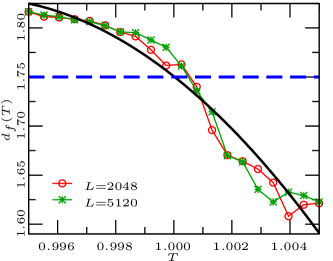
Figure 1: The fractal properties of the $2d$ Ising model. We exhibit the fractal dimension $d_{f}(T)$ as a function of temperature $T$ for a squared lattice with $L=2048$, and $L=5120$. The horizontal dashed blue line is the theoretical value $d_{f}=1.75$ at $T=T_{c}$ . The continuous black line is the the function $f(T)=7/4+a(T-T_{c})+b(T-T_{c})^{2}$, after adjusting to the data

From Eq. (20) we predict $d_{f}=7/4$ for $d=2$ Ising model. At the present stage, we have two possibilities to determine $d_{f}$:

1. To develop theoretical methods to determine $d_{f}$ analytically such as that used recently Gomes-Filho et al. (2021) for the KPZ equation.

2. To use numerical methods Barabasi et al. (1995); Luis et al. (2022); Mozo Luis et al. (2023) to determine it. This is particularly hard close to a phase transition (see supplementary material).

Monte Carlo tests on the Ising model - To obtain numerical values for $d_{f}$, we use a specific box-counting method appropriate for this situation (see supplementary material).

In Fig. 1 we exhibit $d_{f}(T)$ as function of $T$. We use a square lattice and the same procedure as Fig. $S3$. The plots exhibit the data for $L=2048$ and $L=5120$. We observe large fluctuations for $T>1$. As already observed in the supplementary material, the fluctuations above $T_{c}$ are larger than that below, as well, that except for fluctuations, the simulations suggest a universal behavior independent of $L$, for the sizes we have used here. Note that it takes a considerable amount of time to obtain $d_{f}(T)$ as we do not use the CUDA process for the fractal program. Thus we use only a few points around $T_{c}$. As expected the fluctuations are larger in the region close to $T_{c}$, and they decrease as we increase the number of realizations (see table I supplementary material). For $T\approx T_{c}$, $d_{f}(T)\approx f(T)=7/4+a(T-T_{c})+b(T-T_{c})^{2}$, which we use to determine $T_{c}=0.99996\pm 0.00025$ for $L=2048$ and $T_{c}=1.00007\pm 0.0003$ for $L=5120$. Values for $L=1024\times m$, $m=1,2,..6$ are reported in Table I. The results support with good precision our theoretical value $d_{f}=7/4$. Unfortunately, the method is not good for three dimensions.

Conclusion - We have discussed here the correlation function Eq. (2) at a critical point, and we suggest that there is a fractal dimension $d_{f}$ associated with the Fisher exponent as $\eta=d-d_{f}$. We obtain the analytical value $d_{f}=7/4$ for the $2d$ Ising model, which is supported by our simulations.

The Ising model for equilibrium and the KPZ equation for non-equilibrium, are among the most used models in statistical mechanics. It is therefore very encouraging to see that Eq. (10) for growth is equivalent to Eq. (20). Both relationships go beyond KPZ and Ising models in that they show that the deviation from mean field theories when the correlation becomes important can be seen as a deviation from the integer to a fractal dimension describing the spatial distribution of activity.

The major idea supporting this hypothesis is the fact that the fluctuation-dissipation theorem, i.e., response functions, depends on ergodicity Gomes-Filho and Oliveira (2021); Costa et al. (2003); Wen et al. (2023), which is violated when disorder comes into play Lapas et al. (2008). Near the transition, there is a “permanent state of disorder” where the fluctuations play a major role. Furthermore, the correlation function for the fluctuations Eq. (3) is quite general, and not just for the Ising model. Consequently, we hope this result will be confirmed in other systems and have more general application.

In this way, this could signify a new approach to the physics of phase transition, particularly in disordered systems such as spin glass.

Acknowledgments - This work was supported by the Conselho Nacional de Desenvolvimento Científico e Tecnológico (CNPq), Grant No. CNPq-01300.008811/2022-51 and Fundação de Apoio a Pesquisa do Rio de Janeiro (FAPERJ), Grant No. SEI-260003/005791/2022 (E.E.M.L), and Fundação de Apoio a Pesquisa do Rio de Janeiro (FAPERJ), Grant No. E-26/203953/2022 (F.A.O.), and Fundação de Apoio a Pesquisa do Distrito Federal (FAPDF), Grant No. 00193-00001817/2023-43. It was also partly supported by the Research Council of Norway through its Centres of Excellence funding scheme, Project Number 262644 (A.H.).

References

- Devakul et al. (2019) T. Devakul, Y. You, F. J. Burnell, and S. L. Sondhi, SciPost Phys. 6, 007 (2019).
- Strogatz (2000) S. H. Strogatz, Nonlinear Dynamics and Chaos (Perseus Book Publishing, 2000).
- Kardar (2007) M. Kardar, Statistical physics of fields (Cambridge University Press, 2007).
- Cardy (1996) J. Cardy, Scaling and renormalization in statistical physics, Vol. 5 (Cambridge university press, 1996).
- Fisher (1964) M. E. Fisher, Journal of Mathematical Physics 5, 944 (1964).
- dos Anjos et al. (2021) P. H. R. dos Anjos, M. S. Gomes-Filho, W. S. Alves, D. L. Azevedo, and F. A. Oliveira, Frontiers in Physics 9 (2021), 10.3389/fphy.2021.741590.
- Gomes-Filho et al. (2021) M. S. Gomes-Filho, A. L. Penna, and F. A. Oliveira, Results in Physics 26, 104435 (2021).
- Kardar et al. (1986) M. Kardar, G. Parisi, and Y.-C. Zhang, Phys. Rev. Lett. 56, 889 (1986).
- Barabasi et al. (1995) A.-L. Barabasi, H. E. Stanley, et al., Fractal concepts in surface growth (Cambridge university press, 1995).
- Gomes-Filho and Oliveira (2021) M. S. Gomes-Filho and F. A. Oliveira, Europhysics Letters 133, 10001 (2021).
- Mello et al. (2001) B. A. Mello, A. S. Chaves, and F. A. Oliveira, Phys. Rev. E 63, 041113 (2001).
- Reis (2005) F. D. A. A. Reis, Phys. Rev. E 72, 032601 (2005).
- Rodrigues et al. (2014) E. A. Rodrigues, B. A. Mello, and F. A. Oliveira, Journal of Physics A: Mathematical and Theoretical 48, 035001 (2014).
- Alves et al. (2016) W. S. Alves, E. A. Rodrigues, H. A. Fernandes, B. A. Mello, F. A. Oliveira, and I. V. L. Costa, Phys. Rev. E 94, 042119 (2016).
- Carrasco and Oliveira (2018) I. S. S. Carrasco and T. J. Oliveira, Phys. Rev. E 98, 010102 (2018).
- Krug et al. (1992) J. Krug, P. Meakin, and T. Halpin-Healy, Phys. Rev. A 45, 638 (1992).
- Krug (1997) J. Krug, Advances in Physics 46, 139 (1997).
- Derrida and Lebowitz (1998) B. Derrida and J. L. Lebowitz, Phys. Rev. Lett. 80, 209 (1998).
- Meakin et al. (1986) P. Meakin, P. Ramanlal, L. M. Sander, and R. C. Ball, Phys. Rev. A 34, 5091 (1986).
- Daryaei (2020) E. Daryaei, Phys. Rev. E 101, 062108 (2020).
- Edwards and Wilkinson (1982) S. F. Edwards and D. Wilkinson, Proceedings of the Royal Society of London. A. Mathematical and Physical Sciences 381, 17 (1982).
- Hansen et al. (2000) A. Hansen, J. Schmittbuhl, G. G. Batrouni, and F. A. de Oliveira, Geophysical research letters 27, 3639 (2000).
- Wolf and Kertesz (1987) D. Wolf and J. Kertesz, Europhys. Lett. 4, 651 (1987).
- Rodrigues et al. (2024) E. A. Rodrigues, E. E. M. Luis, T. A. de Assis, and F. A. Oliveira, Journal of Statistical Mechanics: Theory and Experiment 2024, 013209 (2024).
- Merikoski et al. (2003) J. Merikoski, J. Maunuksela, M. Myllys, J. Timonen, and M. J. Alava, Phys. Rev. Lett. 90, 024501 (2003).
- Odor et al. (2010) G. Odor, B. Liedke, and K.-H. Heinig, Phys. Rev. E 81, 031112 (2010).
- Takeuchi (2013) K. A. Takeuchi, Phys. Rev. Lett. 110, 210604 (2013).
- Gwa and Spohn (1992) L.-H. Gwa and H. Spohn, Physical review letters 68, 725 (1992).
- De Vega and Woynarovich (1985) H. De Vega and F. Woynarovich, Nuclear Physics B 251, 439 (1985).
- Plischke et al. (1987) M. Plischke, Z. Racz, and D. Liu, Physical Review B 35, 3485 (1987).
- Corwin et al. (2018) I. Corwin, P. Ghosal, A. Krajenbrink, P. Le Doussal, and L.-C. Tsai, Phys. Rev. Lett. 121, 060201 (2018).
- Nahum et al. (2017) A. Nahum, J. Ruhman, S. Vijay, and J. Haah, Phys. Rev. X 7, 031016 (2017).
- Ljubotina et al. (2019) M. Ljubotina, M. Žnidarič, and T. c. v. Prosen, Phys. Rev. Lett. 122, 210602 (2019).
- De Nardis et al. (2019) J. De Nardis, M. Medenjak, C. Karrasch, and E. Ilievski, Phys. Rev. Lett. 123, 186601 (2019).
-
Moca et al. (2023)
C. P. Moca, M. A. Werner,
A. Valli, G. Zar
and, and T. Prosen, arXiv preprint arXiv:2306.11540 (2023). - Rodriguez and Wio (2019) M. A. Rodriguez and H. S. Wio, Phys. Rev. E 100, 032111 (2019).
- Grigera and Israeloff (1999) T. S. Grigera and N. E. Israeloff, Phys. Rev. Lett. 83, 5038 (1999).
- Ricci-Tersenghi et al. (2000) F. Ricci-Tersenghi, D. A. Stariolo, and J. J. Arenzon, Phys. Rev. Lett. 84, 4473 (2000).
- Crisanti and Ritort (2003) A. Crisanti and F. Ritort, Journal of Physics A: Mathematical and General 36, R181 (2003).
- Barrat (1998) A. Barrat, Phys. Rev. E 57, 3629 (1998).
- Bellon and Ciliberto (2002) L. Bellon and S. Ciliberto, Physica D: Nonlinear Phenomena 168, 325 (2002).
- Bellon et al. (2006) L. Bellon, L. Buisson, M. Ciccotti, S. Ciliberto, and F. Douarche, in Jamming, Yielding, and Irreversible Deformation in Condensed Matter (Springer, 2006) pp. 23–52.
- Vainstein et al. (2005) M. Vainstein, R. Morgado, F. Oliveira, F. de Moura, and M. Coutinho-Filho, Physics Letters A 339, 33 (2005).
- Hayashi and Takano (2007) K. Hayashi and M. Takano, Biophysical journal 93, 895 (2007).
- Pérez-Madrid et al. (2009) A. Pérez-Madrid, L. C. Lapas, and J. M. Rubí, Phys. Rev. Lett. 103, 048301 (2009).
- Averin and Pekola (2010) D. V. Averin and J. P. Pekola, Phys. Rev. Lett. 104, 220601 (2010).
- Costa et al. (2003) I. V. L. Costa, R. Morgado, M. V. B. T. Lima, and F. A. Oliveira, Europhysics Letters 63, 173 (2003).
- Costa et al. (2006) I. Costa, M. Vainstein, L. Lapas, A. Batista, and F. Oliveira, Physica A: Statistical Mechanics and its Applications 371, 130 (2006).
- Lapas et al. (2007) L. C. Lapas, I. V. L. Costa, M. H. Vainstein, and F. A. Oliveira, Europhysics Letters 77, 37004 (2007).
- Lapas et al. (2008) L. C. Lapas, R. Morgado, M. H. Vainstein, J. M. Rubí, and F. A. Oliveira, Phys. Rev. Lett. 101, 230602 (2008).
- Gomes-Filho et al. (2023) M. S. Gomes-Filho, L. Lapas, E. Gudowska-Nowak, and F. A. Oliveira, “Fluctuation-dissipation relations from a modern perspective,” (2023), arXiv:2312.10134 [cond-mat.stat-mech] .
- Luis et al. (2022) E. E. M. Luis, T. A. de Assis, and F. A. Oliveira, Journal of Statistical Mechanics: Theory and Experiment 2022, 083202 (2022).
- Mozo Luis et al. (2023) E. E. Mozo Luis, F. A. Oliveira, and T. A. de Assis, Phys. Rev. E 107, 034802 (2023).
- Amorim et al. (2023) P. M. Amorim, E. E. Mozo Luis, F. F. DallAgnol, and T. A. de Assis, Journal of Applied Physics 133, 235304 (2023).
- Bhattacharyya and Chakrabarti (2006) P. Bhattacharyya and B. K. Chakrabarti, Modelling critical and catastrophic phenomena in geoscience: a statistical physics approach, Vol. 705 (Springer, 2006).
- Muslih and Agrawal (2010) S. I. Muslih and O. P. Agrawal, International Journal of Theoretical Physics 49, 270 (2010).
- Muslih (2010) S. I. Muslih, International Journal of Theoretical Physics 49, 2095 (2010).
- Laskin (2007) N. Laskin, Communications in Nonlinear Science and Numerical Simulation 12, 2 (2007).
- Pelissetto and Vicari (2002) A. Pelissetto and E. Vicari, Physics Reports 368, 549 (2002).
- Zhang and March (2012) Z. Zhang and N. March, Journal of Mathematical Chemistry 50, 920 (2012).
- Wen et al. (2023) B. Wen, M.-G. Li, J. Liu, and J.-D. Bao, Entropy 25, 1012 (2023).