Random features and polynomial rules
Abstract
Random features models play a distinguished role in the theory of deep learning, describing the behavior of neural networks close to their infinite-width limit. In this work, we present a thorough analysis of the generalization performance of random features models for generic supervised learning problems with Gaussian data. Our approach, built with tools from the statistical mechanics of disordered systems, maps the random features model to an equivalent polynomial model, and allows us to plot average generalization curves as functions of the two main control parameters of the problem: the number of random features and the size of the training set, both assumed to scale as powers in the input dimension . Our results extend the case of proportional scaling between , and . They are in accordance with rigorous bounds known for certain particular learning tasks and are in quantitative agreement with numerical experiments performed over many order of magnitudes of and . We find good agreement also far from the asymptotic limits where and at least one between , remains finite.
I Introduction
The connection between deep feed-forward neural networks (DNNs) in the large-width limit and kernel methods has been well understood in the last years. It has been shown, in a Bayesian learning perspective, that if the number of units in each hidden layer is taken to infinity at fixed input dimension and training set size, a DNN becomes a “neural network Gaussian process” whose kernels can be defined iteratively layer by layer [1, 2, 3, 4]. This result has been recently generalized beyond the infinite-width limit [5, 6, 7, 8, 9, 10]. In a dynamical perspective moreover, it has been shown that wide DNNs trained with gradient-based methods exhibit a the lazy-training kernel regime [11], evaluated by first order Taylor-expanding the network with respect to the weights around initialization [12, 13, 14].
Once a DNN is proven equivalent to a kernel machine, the mechanism by which it realizes the input-output mapping of the corresponding supervised-learning task is understood: the input data, which generally speaking are points in , are mapped with an implicit feature map to an -dimensional space where the classification, or regression, rule is linear and can be learnt by the read-out layer. The mapping to the feature space is implicit, in the sense that the learning problem can be solved by a support vector machine (SVM), so that learning and generalization depend on the features only through the kernel (see, for reference, [15]). Learning curves (generalization error as a function of the size of the training set) of kernel machines can be obtained analytically from a statistical mechanics [16, 17, 18, 19] or a mathematical [20, 21, 22] perspective. A very interesting trait of these curves is their staircase shape for : by setting the scaling of the size of the training set to a certain power of the input dimension, features of order can be learnt by the machine, so that the test error decreases increasing with subsequent steps.
The discovery of the lazy training regime of wide neural networks motivated in the recent past the study of the random features model (RFM) [23, 24], a shallow (one-hidden-layer, 1HL) neural network where the feature map is explicitly parametrized by a fixed random linear embedding of the input points from to , followed by a non-linear activation function. In this sense, the model mimics the behavior of a neural network in the large-width limit, where the feature map depends only on initialization and learning is linear.
In the present work we study theoretically the generalization performance of the RFM in the large- limit, with , . We find, under a quite general teacher/student setting with a random polynomial teacher and Gaussian i.i.d. input data, that
-
•
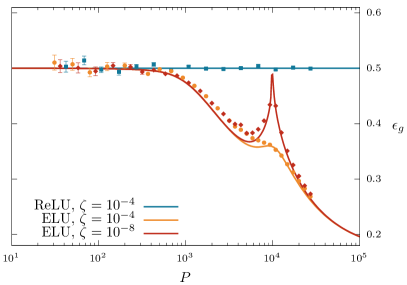
as long as , the model behaves as an infinite-rank () kernel machine: for , features of order can be learnt, such that the generalization error as a function of has a staircase descent (or overfitting peaks if the teacher is less complex) with steps corresponding to different values of ;
-
•
for and , the model is equivalent to a degree- polynomial student: if the complexity of the teacher is lower than the degree , the generalization error is equal to zero, or otherwise, to the minimum error for a degree- polynomial fitting a more complex teacher;
-
•
for , an interpolation peak of the generalization error, which depends on the strength of the regularization of the student’s weights, occurs.
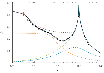
This behavior is depicted in Fig. 1. Comparison with numerical experiments shows that our theory, based on the mapping of the RFM to an equivalent noisy polynomial model, predicts well the quantitative behavior of the true generalization performance at finite size, over many orders of magnitude.
Our theory, formulated from the point of view of the statistical mechanics of disordered systems, expresses the generalization performance of the RFM in terms of few order parameters with a clear physical interpretation, as overlaps between combinations of the student’s weights and the parameters defining the teacher. In this way, we are offering a complementary take on what is known about RFMs in the computer science community, as we discuss in the following.
I.1 Related works
In this section we give an overview on the previous works that have been of inspiration to our paper, presenting relevant results and differences with our approach.
Random feature models were introduced in [24, 23, 25, 26], initially as randomized low-rank approximations of kernels arising in classification or regression problems. Recently, their interest was renewed by the discovery that DNNs behaves as RFMs close to the infinite-width limit, both in a Bayesian learning [1, 2, 3, 4] and in a gradient-based learning [12, 13, 11, 14] setting. This mapping, which provides one of the few limits where DNNs can be studied with analytical methods, has motivated in the last few years a huge effort to formalize their behavior in terms of expressive power and generalization performance.
In particular, the impressive series of works [27, 28, 29, 30, 14, 31, 32, 33] (see [34] for a review) formulates rigorous bounds on the generalization performance of RFMs in different asymptotic regimes. For a non-exhaustive recap of the results (with our notation):
-
•
In [27], the large- limits where (for small ) after sending (underparametrized regime) and after sending (overparametrized regime) are considered. In the first case the model is found equivalent to degree- polynomial regression; in the second one, it reduces to (infinite-rank) kernel regression, which for that number of samples can fit at most a degree- polynomial in the inputs, in a way also investigated in literature [16, 17, 18, 19, 20, 21, 22].
-
•
In [29], the limit where both and scale linearly with with their ratio fixed is considered; the generalization error as a function of the ratio between the number of hidden units and the size of the training set first decreases for small, then exhibits a peak at the interpolation threshold and then relaxes again for to the value predicted from the kernel theory with , coherently with the previous point. This phenomenology is widely observed in numerical experiments and known in literature as double descent [35] of the generalization error.
- •
-
•
In [33], universality results on training and test error are proven in the regime for a larger class of models, as long as with finite-dimensional outputs, and generic losses. Indeed, they prove that training and test errors depend on the random features distribution only through its covariance structure.
These papers find bounds to the generalization performance of a RFM with rigorous analytical methods under quite general assumptions on data distribution and activation functions.
A statistical mechanics point of view, complementary to the formal approach discussed so far, has been formulated in the series of papers [36, 37, 38, 39, 40, 41, 42]. Originally aiming at modelling the role of data structure in machine learning, as in other contemporary approaches [43, 44, 45, 46, 47, 48, 49, 50], the authors obtained in [37] a closed-form expression for the generalization error of RFMs for regression and classification in the asymptotic regime where . Their approach, based on the replica theory from statistical mechanics [51], can be applied to supervised learning tasks with generic convex loss functions. Not only their results are supported under mild hypothesis by analytical proofs [29, 38, 52, 53, 33], but they can predict remarkably well the numerical experiments. Our work extends these results to more general scaling regimes, where , .
One of the main steps in our derivation is the expansion of activation function of the hidden layer on a polynomial basis, which corresponds to the diagonalization of the kernel (19) on its eigenbasis (Mercer’s decomposition). This expansion is then truncated to a certain degree , corresponding to the integer exponent in the scaling law : similar approximations appeared recently in [54, 55]. Moreover, while the literature on the double descent behavior of the generalization error is vast and impossible to outline here (see for example [35]), we mention [56], where the presence of more than one peak in the generalization curve is remarked: the authors call “linear peak” the one occurring at for , where the model behaves as a kernel learning the linear features, while for there is a “non-linear peak” due to the non-linearity of the activation function acting as noise and overfitted when and are of the same order; in the present work we show that, as long as , there is a peak (or a descent) for each of the regimes .
II The Model
| Symbol | Definition |
|---|---|
| input space dimension | |
| feature space dimension | |
| size of the training set | |
| number of replicas | |
| indices in input space | |
| indices in feature space | |
| indices spanning the training set | |
| indices in replica space | |
| multi-index , | |
| , | teacher parameters, |
| random features matrix | |
| , | , |
| , … | , , … |
We would like to study the generalization performance of the Random Features model in a teacher/student [57, 58] supervised learning set-up, where the teacher performs an input-output mapping with various degree of complexity. We summarize in Table 1 the main notations used in this paper.
The input data are vectors in with i.i.d. Gaussian elements, while the labels are assigned by a polynomial teacher of degree defined as:
| (1) | ||||
where is a fixed external parameter (the average value of the teacher, which acts as a bias term), , , are i.i.d. parameters collectively denoted as , describing the non-linear decision boundary (diagonal terms, irrelevant for large , are for simplicity not included in the sum), the mixture parameters , weighting the monomials of different degree, are taken to be subject to . Simple examples of this setting are a deterministic teacher for binary classification or a noisy teacher for polynomial regression with variance of the noise , for which Eq. (1) reduces respectively to
| (2) |
It has been shown in [16] that a polynomial student, defined in the same way as in Eq. (1), would learn the weights of the teacher in a hierarchical fashion: examples are needed in order to learn the parameters for . However, here the student’s task is to learn the weights of the last layer of a 2-layers NN, , whose first layer realizes a random embedding of the data in a -dimensional feature space:
| (3) | ||||
| (4) |
where is a quenched random matrix with i.i.d. standard normal entries, is the non-linear activation function of the hidden layer, the student’s weight vector and the activation function of the last (“readout”) layer. It is customary to introduce the pre-activations
| (5) |
which at fixed instance of the random features , given that we chose i.i.d normal variables, follow a multivariate Gaussian distribution with covariance
| (6) |
In our setting with independent random features, is a Wishart matrix.
While our theory is general in the choice of (as long as it admits an expansion on the basis of Hermite polynomials, as discussed in Sec. IV), we will test our results for popular choices, such as
| (7) | ||||
| (8) |
(respectively, Rectified and Exponential Linear Unit).
The training set is made of input-output pairs, . The student learns by solving the following optimization problem,
| (9) |
where is an opportune convex loss function and controls the regularization of the weights. The choice of the loss function and the readout activation function in Eq. (3) defines the specific learning task to perform. While our theory is generic, to simplify calculations we will mostly look at the case of a pure quadratic loss
| (10) |
which corresponds to a regression task () or a binary classification task (); the use of a regression loss for a classification task dates back to the early days of NNs [59, 58].
The main aim of this work is the evaluation of the generalization performance of the model, both for the classification and the regression problems, using a statistical mechanics approach. From this perspective, the model defines a disordered system with degrees of freedom , and quenched disorder given by the realization of the training set , the teacher’s parameters and the random features . Our computation will follow the standard path, starting from the computation partition function at inverse temperature
| (11) |
III Generalization error
In order to quantify how well the student can learn the teacher, we look at the generalization error, defined as the probability of misclassifying a new sample (in the case of classification) or as the mean squared error of a new point (in the case of regression). Given a test point , both cases can be expressed with the following formula,
| (12) |
where for binary classification and for regression. With (12) we can evaluate the quality of the student NN (3) for a given realization of the teacher, of the random weights , and of the dataset . In order to get a general view of the effectiveness of (3), we calculate the average generalization error over all the sources of randomness. Doing so, we get a function of , , and only,
| (13) | ||||
where we took .
We have written the average generalization error as in Eq. (13) to show that we only need to know the joint distribution of to evaluate it. Being a test point, and so uncorrelated from , by central limit theorem we can treat the distribution as Gaussian: to compute the generalization error we only need the first and second moments,
| (14) | ||||||
Notice that by definition of the model is identically equal to 1. In section V we will show how to obtain this quantities from a replica approach.
For the case of binary classification with ,
| (15) | ||||
where we use the Gardner notation [57] and . Notice that when (that is, when both teacher and student are zero-mean) the formula simplifies to
| (16) |
For the case of polynomial regression () [60, 61],
| (17) |
These formulas remind the generalization error of a generalized linear model with the same architecture as the teacher [58]: in that case, corresponds to the angle between the teacher and the student weight vectors. For the RFM, it is not clear a priori if we can interpret as a scalar product of the teacher’s weight vector and some effective weights of the student. If this can be done, the RFM could be mapped to an equivalent polynomial model. In Sec. IV we will show how to explicitly construct it from and , thus achieving this mapping. To do so, we need to spend a few words on the connection between RFMs and kernel machines, in order to explain the truncation of the activation function on the basis of Hermite polynomials, which we will use later on.
IV Kernel learning and polynomial models
The RFM defined in (3) is a generalized linear model in the learnable parameters , so it can be formulated as a kernel model, as we remind in this section. First of all, in the particular choice of quadratic loss, one can write down an explicit formula for the solution of (9),
| (18) |
where the pre-activations are given by (5) and the operator
| (19) |
defines the kernel in feature space.
More in general, for arbitrary loss, the optimization problem (9) admits a dual representation in terms of slack parameters (forces) that enforce the condition . This is easily seen writing the minimization of the loss as a constrained optimization problem
| (20) | ||||
and solving it eliminating the in favour of Lagrange multipliers
| (21) |
where
| (22) |
defines the kernel in input space. The equivalence between the two formulations can also be seen noticing that .
From Eq. (19) it is possible to obtain an explicit formula of the kernel as a function of the covariance matrix of the pre-activations (6). To this aim, as the preactivations are Gaussian, it is convenient to expand the activation function on the basis of Hermite polynomials (see also [27]):
| (23) |
where is the -th Hermite polynomial and the coefficient can be evaluated using orthogonality of the Hermite basis, , so that
| (24) |
Along these lines, the kernel (19) can be expressed for large [62, 63] (see App. A for details) as
| (25) |
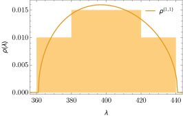
where , given by (6), is a rank Wishart matrix with elements and for . The matrix with entries , which we denote by , defines an interesting random matrix ensemble, obtained taking Hadamard (element by element) powers of the covariance . A similar ensemble was recently studied in [64].
This analysis can be pushed a step forward when the relation between and is fixed: with . Let us note that the matrix has generically rank equal to and off-diagonal elements . We therefore obtain a fully ranked matrix if we truncate the expansion at the minimum value such that . It is clear that while the terms with should be retained to have a positive defined matrix, for the successive terms one can retain the diagonal terms only (equal to 1) and neglect the non-diagonal ones. This will have only a marginal effect on eigenvalues and eigenvectors of the matrix. We can therefore approximate
| (26) |
where
| (27) |
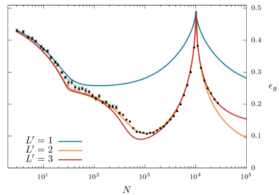
This truncation, which we justified here with an heuristic argument, is proven rigorously for (that is, in the proportional regime ) in [65], and extended to the case under generic assumptions on the kernel in [31, 55]. A convincing check of this property is given by Fig. 1, right: theoretical curves of the generalization error obtained truncating the effective theory described below at different values of are compared with the numerical experiments, as a function of ; quantitative agreement is obtained for , with the numerical points interpolating nicely the theoretical curves in the various regimes.
The analysis above suggests that in the regime we can substitute the RFM with an effective noisy polynomial student
| (28) | ||||
where the student parameters are the scalar product of with the “vectors” with components (see Table 1),
| (29) |
while the last term is a Gaussian noise term with zero mean and variance which can be represented as
| (30) |
in terms of i.i.d. variables . Although the parameters and are functions on the network weights, to enlighten the notation we will not explicitly write the dependence on .
Moreover, we can notice that for fixed , the different monomials, which have unit variance and, sharing the same , are in principle not independent, are only very weakly correlated. In fact, it is clear that for , where we introduced the multi-index notation with (the value of will be clear from the context), while higher order correlation function are vanishing for large . For example . Moreover, the collection of the for different ’s span spaces of very different dimensions, of order , which can be considered approximately orthogonal. As a consequence, the projections of the vector on such spaces can be treated as independent in the analysis of the partition function of the system.
In (28) we give an alternative description of the RFM, mapping it to a polynomial model with correlated weights and noise coming from the terms in the expansion (23). This is an extension to generic scaling regimes of the Gaussian equivalence principle from [38] and related works, to which it reduces when . In the following, we will base our analysis on this representation of . This description makes more transparent the meaning of the observables introduced in Sec. III and the mechanism by which the RFM learns the teacher’s features, as we explain in the following.
V Replica calculation
To obtain the generalization error from a replica approach, we can write the joint probability distribution of and in Eq. (13) as the zero temperature limit of the equilibrium distribution of a statistical mechanics system, as
| (31) |
Through a standard application of the replica trick we rewrite the distribution as
| (32) |
which can be obtained from the calculation of the -times replicated partition function
| (33) |
In this integral, we treat the distribution of and conditioned by , and as Gaussian, with moments given by
| (34) | ||||
Using the representation (28) we can explicitly write (see Appendix B for details)
| (35) | ||||
with the definitions
| (36) | ||||||
where we are using the notation
| (37) |
In the following we will take the approximation
| (38) |
This equation is not exactly equivalent to (36), as here the multi-index is ordered (see Table 1), while in the matrix element it is not. In writing
| (39) |
we are neglecting lower-rank terms that could in principle interfere with terms in for . For a thorough discussion on the approximation we are taking here, see Appendix C.2.
Enforcing these definition with delta functions in Fourier representation, and anticipating saddle point integration for the various and , and their Fourier conjugated parameters that we denote as and with the due indexes, we rewrite the partition function as
| (40) | ||||
where now , the sums over span , and
| (41) |
In writing Eq. (40), we took , as the Fourier conjugate of the mean is suppressed in the large- limit [66] (a property that could be checked a posteriori from the saddle point equation for ); moreover, the conventional scalings with and in this equation are chosen in such a way that the hat variables corresponding to the asymptotic regimes explained in Sec. VI have a non-trivial high-dimensional limit.
Averaging over the we obtain:
| (42) | ||||
and integrating over ,
| (43) | ||||
where traces are taken over replica and feature indices and we introduced for compactness the matrices in replica indices
| (44) | ||||
We notice at this point that, given , for the matrices have rank , and have eigenvalues of order . Simple perturbation theory shows that adding these matrices with coefficients of order 1 only slightly modify the eigenvalues. This is due to the fact that the row spaces (that is, the complements to their null spaces) corresponding to the different are almost orthogonal. In such a situation we approximate the trace-log term appearing in (43) as
| (45) | ||||
(notice that the first is over replica indices only). We report a detailed derivation of Eq. (45) under the hypothesis of orthogonality of the row spaces in Appendix D. Notice that we could have gotten to the same result decomposing the vectors on the row spaces of the supposed orthogonal. This decomposition clearly shows the hierarchical nature of learning.
V.1 Replica symmetric theory
In order to complete the evaluation of the partition function, we need to specify the form of the replica parameters. In this paper we use the replica symmetry (RS) ansatz
| (46) |
Notice that the diagonal elements of the matrix are . The scaling with of the variables can be rationalized considering that in the replica approach these quantities measure the variance of the variables evaluated in the space of the equilibrium configurations of the weights , space that for large shrinks to the unique solution of the optimization problem (10), supposed convex. This implies the following form for the conjugate order parameters in the RS:
| (47) |
Exploiting the explicit parametrization of the RS matrices, we can perform the traces over replica indices in Eq. (45), to get (see Appendix E)
| (48) | ||||
where and traces are over feature indices only.
Using standard properties of Wishart matrices (see Appendix C.1), we can write
| (49) |
where is the Stieltjes transformation of the Marchenko-Pastur distribution with ratio :
| (50) |
Re-arranging terms we get, for large ,
| (51) |
where
| (52) | ||||
and, in the special case of quadratic loss,
| (53) |
where is the average over the teacher distribution (1) and
| (54) | ||||||
A detailed derivation of the terms and , with the form of valid for generic loss functions, is reported in Appendix F.
Eq. (54) gives the RS version of Eq. (35): these quantities are precisely the ones appearing in Eq. (14), giving the low-order statistics of the distribution used to evaluate the generalization error. Once their value is known from the saddle point equations implicit in the derivation of the partition function, they can be used to obtain the generalization curves reported in this paper.
V.2 Saddle-point equations for quadratic loss
The free energy in Eq. (51) has to be evaluated at the saddle point with respect to all the RS order parameters and their Fourier conjugates. The resulting equations, which we report here for the case of quadratic loss function, can be solved in steps. First, a set of nonlinear equations is used to determine the variables and :
| (55) | ||||||
From the solution of Eq. (55), we can fully determine according to
| (56) |
With all the previous values we can determine the rest of the variables through the following set of linear equations:
| (57) | ||||
| (58) | ||||
Notice that, because of the conventional scalings we chose for the hat variables starting from Eq. (40) and for the definition of , these equations give results for the order parameters , , .
By numerically integrating Eq. (55), (56), (57), we obtain the theoretical curves for the generalization error in Eq. (16) and for the order parameters we report in this paper. We compare the result with numerical simulations: despite its asymptotic nature and the hypothesis of row space orthogonality, our theory works reasonably well even if is not large. The results are shown in Fig. 1 ( in this case), where the generalization error is quantitatively predicted by the theory both when varying and .
VI Asymptotic regimes
Our analysis enables us to consider the following asymptotic limits:
-
(i)
, , finite;
-
(ii)
, finite, finite;
-
(iii)
, , finite.
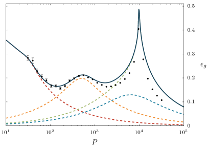
In all of these cases, most of the order parameters go to trivial limits, while only the ones corresponding to the selected scaling converge to non-trivial values. We report the corresponding equations in Appendix G. In this way, we are able to plot the dashed lines in Fig. 1 and 2.
VII Effective theory for finite-size random features networks

In the last sections we devised a theory able to capture the relevant phenomenology of generalization in RFMs at finite values of input dimension, hidden layer width and size of the training set. Indeed, even though the asymptotic approximation leading to the system of saddle-point equations (55), (56), (57) is justified only for large and finite, the curves obtained by fixing the values of , and at finite values are in accordance with numerical simulations over several orders of magnitudes of the control parameters. This occurs thanks to the fact that we kept into account quantities that scale differently with , as or , that are formally zero or infinity in the asymptotic regimes presented in Sec. VI.
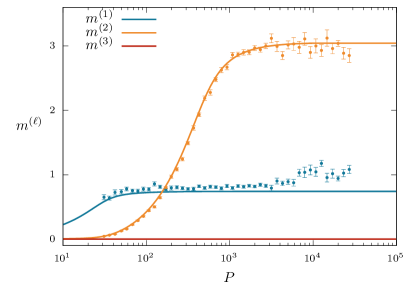
By developing a theory from Eq. (28), we show that the RFM is in essence equivalent to a polynomial model: the student tries to tune its weights through the combinations defined in (29) to fit the corresponding coefficients of the teacher. This interpretation is also confirmed in the numerical experiments: see Fig. 2 (left) for the behavior of the teacher-student overlaps in the case of a quadratic teacher.
However, a crucial difference from a purely polynomial setting arises: the degree of the equivalent polynomial model is controlled by the scaling of the random features, and higher order terms in the expansion of the kernel on the Hermite basis act as noise, given by Eq. (30). This eventually produces the interpolation peak in the generalization error at , which would not be present for a vanilla polynomial student (see Fig. 1 and 2): in this regime, the model is overfitting the effective noise. In terms of the order parameters, overlaps of different orders are coupled by an additional set of parameters , , , related to the noise term in the equivalent polynomial model.
In summary, the learning of features of a certain order is possible as long as the number of parameters is enough: the scaling controls the learning process through the truncation of the kernel (26). At the same time, also plays an important role: if is smaller than , the model only learns as a -degree polynomial; on the other hand, if , the model learns as a -degree polynomial.
By choosing a polynomial teacher of arbitrary degree , we are able to explore to some extent the interplay between the complexity of the data and the one of the neural network. In the case when the teacher is less complex than the network, we can see that overfitting can occur and that overparametrization is not always optimal. This can be seen in the left panel of Fig. 3. In the case of a linear teacher, if the amount of data is , an overparametrized network generalizes better. However, as soon as hits the quadratic regime, but is still far from enabling the network to realize that there is no quadratic feature, then overparametrization leads to overfitting and therefore the optimal is less than .
Interestingly, in order for the model to learn features of order , the activation function must have a non-zero Hermite coefficient in Eq. (23). This can be seen from our theory by the fact that in the total teacher-student overlap in Eq. (54) the single entry is weighted by the corresponding coefficient. This theoretical prediction was tested by using a cubic teacher and two different students, one with ReLU activation function and the other one with ELU: the ReLU one, which has no third order term in the Hermite basis () could not learn the teacher, while the ELU one, that does have a nonzero component (), was able to (see Fig. 3, right).
VIII Conclusions and perspectives
The approach we have explored so far provides a way to analytically evaluate the generalization performance of a RFM in the limit of large input dimension , in the scaling regimes , .
We considered a teacher-student setting, where a shallow random features student is required to fit a polynomial teacher. The student network learns as an equivalent polynomial model with effective noise. We showed this property by expanding the kernel in feature space on a convenient basis (23).
The resulting theory is effective, in the sense that it is formulated in terms of a few collective order parameters (the teacher-student overlaps , the student-student overlaps , ) with a clear physical interpretation and whose values are fixed via a variational principle, as explained in Sec. V. To perform the calculation we neglect the correlations between the student’s coefficients, assuming orthogonality between the row spaces of the components of the kernel.
We find quantitative agreement with numerical simulations, except close to the interpolation peak at in some cases (see Fig. 2, right, where this effect is more apparent). Nevertheless, even then the effective theory gives a good qualitative picture, predicting the location and the shape of the peak. See also Fig. 2, left, depicting how the teacher-student overlaps of already learned features become noisy in the interpolation regime. A precise finite-size analysis of this effect, to address the gap between theory and numerics in this regime, is left for future work.
One possible direction to continue this work is to consider how close is the learning of a fully-trained network to this model. The role of the variables could play a similar role even if the values for are also learned, at least close to the lazy regime. However, what is the fate of row space orthogonality of the kernel components, which is ultimately responsible for the staircase behavior of the generalization error, for networks that are trained end-to-end in a feature learning regime?
Moreover, it would be interesting to extend our analysis to deeper models [10, 67] in different scaling regimes of the dimensions. Even if the RFM, whatever the activation function of the last layer, is essentially bounded by a polynomial model, the precise shape of the kernel and the form of its Mercer’s decomposition in cases where a deeper architecture is involved could help understanding to some extent the feature learning regimes of realistic models, in view of the discussion above.
Acknowledgements
The authors have been supported by a grant from the Simons Foundation (grant No. 454941, S. Franz), thanks to which most of this work was performed at LPTMS (CNRS, Université Paris-Saclay).
FAL conducted part of this research within the Econophysics & Complex Systems Research Chair, under the aegis of the Fondation du Risque, the Fondation de l’École polytechnique, the École polytechnique and Capital Fund Management.
The authors would like to thank Pietro Rotondo, Rosalba Pacelli, Bruno Loureiro, Valentina Ros, the QBio group at ENS for discussions and suggestions. MP and FAL are grateful to the organizers and speakers of the Statistical Physics of Deep Learning summer school held in June 2022 in Como, where the idea was in part conceived.
Appendix A Kernel on the Hermite basis
In this section we report the steps needed to obtain the expression of the feature-feature kernel in Sec. IV. The kernel to evaluate is defined as
| (59) | ||||
where
| (60) |
Using the fact that , this kernel can be written as a series of separable kernels exploiting Mehler’s formula [62, 63], that we report here for convenience:
| (61) |
from which we find Eq. (25) using the fact that, by orthogonality of the Hermite polynomials,
| (62) |
Mehler’s formula, which dates back to 1866, is an example of Mercer’s decomposition [15].
Appendix B Evaluation of the moments of the uniform Gaussian equivalence
We assume that the variables are normally distributed with mean and covariance
| (63) | ||||
where
| (64) | ||||
To proceed, we make the following steps, starting from the expansion of the activation function on the Hermite basis, Eq. (23). For we simply observe that . For we use the fact that is distributed as a standard normal random vector. To deal with we introduce the truncation of (26). Finally, for we need to use the following properties of Hermite polynomials and Gaussian variables,
| (65) |
and using the explicit form of the Hermite polynomials,
| (66) | ||||
we perform Wick’s contractions in order to evaluate the expected value. As the indices are strictly ordered, they must be paired only with ones, so that must be smaller than to give a non-zero contribution. The number of ways we can contract different Gaussian variables with ones is
| (67) |
The remaining variables can be contracted between themselves in
| (68) |
ways. At fixed and and for , even, the only cases different from 0, the sum
| (69) | ||||
is different from 0 and equal to 1 only if . The result is
| (70) | ||||
from which Eq. (35) follows.
Appendix C Results on random matrix theory
C.1 Marchenko-Pastur distribution and Stieltjes transformation
In this section, we remind some textbook results in Random Matrix Theory we used in the main text, for the reader’s convenience. First of all, random matrices of the form
| (71) |
where is a random matrix with i.i.d. entries such that , , define the Wishart (or Wishart-Laguerre) ensemble. For large and , parameter finite, their spectral density follows the Marchenko-Pastur (MP) distribution,
| (72) |
with
| (73) |
with support in .
The MP distribution can be obtained with standard methods [68, 69]. The determinant of the resolvent can be evaluated as follows:
| (74) |
By Gaussian linearization,
| (75) |
The average over gives
| (76) |
Integrating over ,
| (77) |
Inserting with a Dirac delta, we can integrate over :
| (78) |
The integral over the Fourier variable can be solved via asymptotic integration, the saddle-point being in :
| (79) |
The saddle point equation in gives
| (80) |
with solutions
| (81) |
The correct branch can be proven to be . From this analysis, the relation
| (82) |
follows. Deriving with respect to ,
| (83) |
By definition of Stieltjes transformaiton, , which gives Eq. (50).
C.2 Spectral density of
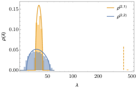
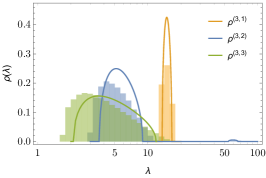
In this section we report some results on the spectral density of the matrices , to clarify the kind of approximation we used in the main text. The analysis will be heuristic. Take, to fix ideas, , so that we consider the matrices
| (84) | ||||
where (we use the label , where is the corresponding exponent in , and the number of different summation indices)
| (85) | ||||
We can say the following on the matrices when , are both (generically) large:
-
•
has a Marchenko-Pastur (MP) spectrum with parameter and , with bulk eigenvalues (and zero eigenvalues).
-
•
can be written, ignoring linear terms, as
(86) where . Notice that . From this, it follows that has an MP spectrum with parameter and , with bulk eigenvalues , plus an additional outlier eigenvalue of order (due to the finite mean); however, in this matrix is scaled by an additional factor of , so it contributes to the sum with eigenvalues and an outlier .
-
•
has an MP spectrum with parameter and , with bulk eigenvalues .
-
•
has an MP spectrum with parameter and , with bulk eigenvalues ; however, in this matrix is scaled by an additional factor of , so it contributes to the sum with eigenvalues .
-
•
can be written, again ignoring linear terms in the matrices , as
(87) The first addendum (notice that the double sum is not symmetric) has an MP spectrum with parameter and , with eigenvalues , while the second addendum is ; however, in they are both scaled by a factor , so they contribute to the sum with eigenvalues and with eigenvalues .
-
•
has an MP spectrum with parameter and , with bulk eigenvalues .
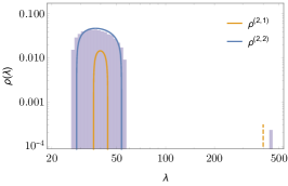
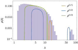
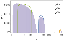
This heuristics is compared with numerical results in Fig. 4, which shows a remarkable accordance. In the main text, we took the approximation , and considered the row spaces of for different as orthogonal: in Fig. 4, bottom right, we show how the spectrum of a sum of the full matrices is reasonably approximated by the sum of the (analytical) spectra of the corresponding matrices, validating our approach.
Appendix D Determinant of sum of matrices with orthogonal row spaces
In this section we prove Eq. (45). Let us take the matrix given by
| (88) |
where the matrices are such that , and their row spaces (that is, the orthogonal complements to their null spaces) are mutually orthogonal ( for ). Then,
| (89) |
where is the determinant restricted to the row space of :
| (90) |
with the non-zero eigenvalues of . Eq. (89) can be proven by noticing that, if is a basis of and a basis of , the set is a basis of in which the matrix is in block-diagonal form. Moreover, from Eq. (90)
| (91) |
so we can conclude that
| (92) |
Appendix E Traces over RS matrices
In this section we prove Eq. (48). We need to evaluate
| (93) |
where , are RS matrices. We can write
| (94) |
where the Kronecker sum is defined as
| (95) |
The eigenvalues of a Kronecker sum are the sums of the eigenvalues of the addenda. Calling the eigenvalues of and the eigenvalues of , this means that
| (96) |
Given that is RS, it has 2 different eigenvalues, with multiplicity and with multiplicity 1, so that for small
| (97) |
In total we get
| (98) |
Using the RS algebra, we know that , , so that
| (99) | ||||
It only remains to find , , , :
| (100) | ||||||
We define to get Eq. (48).
Appendix F Replica-symmetric free energy
In this section we report the main steps to obtain the terms and in Eq. (52) and (53), that is the measure and pattern contributions to the free energy.
F.1 Measure contribution
F.2 Pattern contribution
Appendix G Asymptotic limits of the saddle-point equations
The system of saddle-point equations can be studied in different asymptotic limits:
-
(i)
, , finite;
-
(ii)
, finite, finite;
-
(iii)
, , finite.
G.1 Case (i)
In the limit where scales faster to infinity than , Eq. (55) reduces to
| (106) | ||||
where we used the asymptotic results for the Stieltjes transformation of the Marchenko-Pastur distribution,
| (107) |
Notice that now, consistently,
| (108) |
because recombines with the terms coming from to give . Eq. (56) reduces to
| (109) | ||||
while Eq. (57) becomes
| (110) | ||||
where now
| (111) | ||||
G.2 Case (ii)
In the limit where both and scale in the the same way, , we have, for ,
| (112) | ||||||||
For the other parameters we need to solve the equations for
| (113) | ||||||
for , ,
| (114) |
and for
| (115) | ||||
The values , and are consistent with their definition. At variance with case (i), and have non-trivial values, responsible for the interpolation peak appearing in this regime. Notice that their value is controlled explicitly by the regularizer : the lower it is, the sharper is the peak. Moreover, the spectral function relative to the active component, , also gives a non-trivial contribution.
G.3 Case (iii)
In the limit where is scaling faster than to infinity, we have that for all the order parameters behave as in Eq. (112), meaning that the degree- student learns perfectly all the terms of the teacher of degree less then , as the amount of training data is effectively infinite. In this case
| (116) |
and we have , ; , and
| (117) | ||||
Appendix H Numerical experiments
All numerical experiments were done in Python using JAX, [70], to generate the synthetic random data, and scikit, [71], to optimize the parameters. The optimizer has a simple analytic form given by (18). Nevertheless, it is potentially inefficient to implement the formula naively, as it would require the inversion of a very large matrix. Since we used very large values of and , we decided to perform the ridge regression with the function sklearn.linear_model.Ridge. In this way we could explore regimes of up to order .
Almost all numerical experiments were performed with . In most of the simulations we sampled 50 times for each combination of . For the left panel of Figure 3 we used a larger number of samples since in that case both and were small, hence the generalization error had higher variability. For we used samples respectively for . For we used samples respectively for .
A GitHub repository collecting the code needed to reproduce the figures of this paper (both numerical experiments and theoretical curves from the integration of the saddle-point equations) can be found at [72].
References
- Neal [1996] R. M. Neal, Priors for infinite networks, in Bayesian Learning for Neural Networks (Springer New York, New York, NY, 1996) pp. 29–53.
- Williams [1996] C. Williams, in Advances in Neural Information Processing Systems, Vol. 9, edited by M. Mozer, M. Jordan, and T. Petsche (MIT Press, 1996).
- Lee et al. [2018] J. Lee, J. Sohl-dickstein, J. Pennington, R. Novak, S. Schoenholz, and Y. Bahri, in International Conference on Learning Representations (2018).
- de G. Matthews et al. [2018] A. G. de G. Matthews, J. Hron, M. Rowland, R. E. Turner, and Z. Ghahramani, in International Conference on Learning Representations (2018).
- Naveh and Ringel [2021] G. Naveh and Z. Ringel, in Advances in Neural Information Processing Systems, Vol. 34, edited by M. Ranzato, A. Beygelzimer, Y. Dauphin, P. Liang, and J. W. Vaughan (Curran Associates, Inc., 2021) pp. 21352–21364.
- Ariosto et al. [2022a] S. Ariosto, R. Pacelli, F. Ginelli, M. Gherardi, and P. Rotondo, Phys. Rev. E 105, 064309 (2022a), 2201.11022 .
- Ariosto et al. [2022b] S. Ariosto, R. Pacelli, M. Pastore, F. Ginelli, M. Gherardi, and P. Rotondo, Statistical mechanics of deep learning beyond the infinite-width limit (2022b).
- Atanasov et al. [2022] A. Atanasov, B. Bordelon, S. Sainathan, and C. Pehlevan, The onset of variance-limited behavior for networks in the lazy and rich regimes (2022).
- Seroussi et al. [2023] I. Seroussi, G. Naveh, and Z. Ringel, Nature Communications 14, 908 (2023).
- Cui et al. [2023] H. Cui, F. Krzakala, and L. Zdeborová, Optimal learning of deep random networks of extensive-width (2023).
- Chizat et al. [2019] L. Chizat, E. Oyallon, and F. Bach, in Advances in Neural Information Processing Systems, Vol. 32, edited by H. Wallach, H. Larochelle, A. Beygelzimer, F. d'Alché-Buc, E. Fox, and R. Garnett (Curran Associates, Inc., 2019).
- Jacot et al. [2018] A. Jacot, F. Gabriel, and C. Hongler, in Advances in Neural Information Processing Systems, Vol. 31, edited by S. Bengio, H. Wallach, H. Larochelle, K. Grauman, N. Cesa-Bianchi, and R. Garnett (Curran Associates, Inc., 2018).
- Bietti and Mairal [2019] A. Bietti and J. Mairal, in Advances in Neural Information Processing Systems, Vol. 32, edited by H. Wallach, H. Larochelle, A. Beygelzimer, F. d'Alché-Buc, E. Fox, and R. Garnett (Curran Associates, Inc., 2019).
- Montanari and Zhong [2022] A. Montanari and Y. Zhong, The Annals of Statistics 50, 2816 (2022), 2007.12826 .
- Cristianini and Shawe-Taylor [2000] N. Cristianini and J. Shawe-Taylor, An Introduction to Support Vector Machines and Other Kernel-based Learning Methods (Cambridge University Press, 2000).
- Yoon and Oh [1998] H. Yoon and J.-H. Oh, Journal of Physics A: Mathematical and General 31, 7771 (1998).
- Dietrich et al. [1999] R. Dietrich, M. Opper, and H. Sompolinsky, Phys. Rev. Lett. 82, 2975 (1999).
- Bordelon et al. [2020] B. Bordelon, A. Canatar, and C. Pehlevan, in Proceedings of the 37th International Conference on Machine Learning, Proceedings of Machine Learning Research, Vol. 119, edited by H. D. III and A. Singh (PMLR, 2020) pp. 1024–1034, 2002.02561 .
- Canatar et al. [2021] A. Canatar, B. Bordelon, and C. Pehlevan, Nature Communications 12, 2914 (2021), 2006.13198 .
- Misiakiewicz [2022] T. Misiakiewicz, Spectrum of inner-product kernel matrices in the polynomial regime and multiple descent phenomenon in kernel ridge regression (2022).
- Hu and Lu [2022] H. Hu and Y. M. Lu, Sharp asymptotics of kernel ridge regression beyond the linear regime (2022).
- Xiao and Pennington [2022] L. Xiao and J. Pennington, Precise learning curves and higher-order scaling limits for dot product kernel regression (2022).
- Rahimi and Recht [2007] A. Rahimi and B. Recht, in Advances in Neural Information Processing Systems, Vol. 20, edited by J. Platt, D. Koller, Y. Singer, and S. Roweis (Curran Associates, Inc., 2007).
- Balcan et al. [2006] M.-F. Balcan, A. Blum, and S. Vempala, Machine Learning 65, 79 (2006).
- Rahimi and Recht [2008a] A. Rahimi and B. Recht, in Advances in Neural Information Processing Systems, Vol. 21, edited by D. Koller, D. Schuurmans, Y. Bengio, and L. Bottou (Curran Associates, Inc., 2008).
- Rahimi and Recht [2008b] A. Rahimi and B. Recht, in 2008 46th Annual Allerton Conference on Communication, Control, and Computing (2008) pp. 555–561.
- Ghorbani et al. [2021] B. Ghorbani, S. Mei, T. Misiakiewicz, and A. Montanari, The Annals of Statistics 49, 1029 (2021), 1904.12191 .
- Ghorbani et al. [2019] B. Ghorbani, S. Mei, T. Misiakiewicz, and A. Montanari, in Advances in Neural Information Processing Systems, Vol. 32, edited by H. Wallach, H. Larochelle, A. Beygelzimer, F. d'Alché-Buc, E. Fox, and R. Garnett (Curran Associates, Inc., 2019) 1906.08899 .
- Mei and Montanari [2022] S. Mei and A. Montanari, Communications on Pure and Applied Mathematics 75, 667 (2022), 1908.05355 .
- Ghorbani et al. [2020] B. Ghorbani, S. Mei, T. Misiakiewicz, and A. Montanari, in Advances in Neural Information Processing Systems, Vol. 33, edited by H. Larochelle, M. Ranzato, R. Hadsell, M. Balcan, and H. Lin (Curran Associates, Inc., 2020) pp. 14820–14830, 2006.13409 .
- Mei et al. [2022] S. Mei, T. Misiakiewicz, and A. Montanari, Applied and Computational Harmonic Analysis 59, 3 (2022), special Issue on Harmonic Analysis and Machine Learning, 2101.10588 .
- Mei et al. [2021] S. Mei, T. Misiakiewicz, and A. Montanari, in Proceedings of Thirty Fourth Conference on Learning Theory, Proceedings of Machine Learning Research, Vol. 134, edited by M. Belkin and S. Kpotufe (PMLR, 2021) pp. 3351–3418, 2102.13219 .
- Montanari and Saeed [2022] A. Montanari and B. N. Saeed, in Proceedings of Thirty Fifth Conference on Learning Theory, Proceedings of Machine Learning Research, Vol. 178, edited by P.-L. Loh and M. Raginsky (PMLR, 2022) pp. 4310–4312.
- Bartlett et al. [2021] P. L. Bartlett, A. Montanari, and A. Rakhlin, Acta Numerica 30, 87–201 (2021).
- Belkin et al. [2019] M. Belkin, D. Hsu, S. Ma, and S. Mandal, Proceedings of the National Academy of Sciences 116, 15849 (2019).
- Goldt et al. [2020] S. Goldt, M. Mézard, F. Krzakala, and L. Zdeborová, Phys. Rev. X 10, 041044 (2020), 1909.11500 .
- Gerace et al. [2021] F. Gerace, B. Loureiro, F. Krzakala, M. Mézard, and L. Zdeborová, Journal of Statistical Mechanics: Theory and Experiment 2021, 124013 (2021), 2002.09339 .
- Goldt et al. [2022] S. Goldt, B. Loureiro, G. Reeves, F. Krzakala, M. Mezard, and L. Zdeborova, in Proceedings of the 2nd Mathematical and Scientific Machine Learning Conference, Proceedings of Machine Learning Research, Vol. 145, edited by J. Bruna, J. Hesthaven, and L. Zdeborova (PMLR, 2022) pp. 426–471, 2006.14709 .
- Loureiro et al. [2021] B. Loureiro, C. Gerbelot, H. Cui, S. Goldt, F. Krzakala, M. Mezard, and L. Zdeborová, in Advances in Neural Information Processing Systems, Vol. 34, edited by M. Ranzato, A. Beygelzimer, Y. Dauphin, P. Liang, and J. W. Vaughan (Curran Associates, Inc., 2021) pp. 18137–18151, 2102.08127 .
- Refinetti et al. [2021] M. Refinetti, S. Goldt, F. Krzakala, and L. Zdeborova, in Proceedings of the 38th International Conference on Machine Learning, Proceedings of Machine Learning Research, Vol. 139, edited by M. Meila and T. Zhang (PMLR, 2021) pp. 8936–8947, 2102.11742 .
- Cui et al. [2021] H. Cui, B. Loureiro, F. Krzakala, and L. Zdeborova, in Advances in Neural Information Processing Systems, edited by A. Beygelzimer, Y. Dauphin, P. Liang, and J. W. Vaughan (2021) 2105.15004 .
- Schröder et al. [2023] D. Schröder, H. Cui, D. Dmitriev, and B. Loureiro, in Proceedings of the 40th International Conference on Machine Learning, Proceedings of Machine Learning Research, Vol. 202, edited by A. Krause, E. Brunskill, K. Cho, B. Engelhardt, S. Sabato, and J. Scarlett (PMLR, 2023) pp. 30285–30320.
- Chung et al. [2016] S. Chung, D. D. Lee, and H. Sompolinsky, Phys. Rev. E 93, 060301 (2016), 1512.01834 .
- Chung et al. [2018] S. Chung, D. D. Lee, and H. Sompolinsky, Phys. Rev. X 8, 031003 (2018), 1710.06487 .
- Borra et al. [2019] F. Borra, M. C. Lagomarsino, P. Rotondo, and M. Gherardi, Journal of Physics A: Mathematical and Theoretical 52, 384004 (2019), 1903.06818 .
- Rotondo et al. [2020a] P. Rotondo, M. C. Lagomarsino, and M. Gherardi, Phys. Rev. Res. 2, 023169 (2020a), 1903.12021 .
- Rotondo et al. [2020b] P. Rotondo, M. Pastore, and M. Gherardi, Phys. Rev. Lett. 125, 120601 (2020b), 2005.09992 .
- Pastore et al. [2020] M. Pastore, P. Rotondo, V. Erba, and M. Gherardi, Phys. Rev. E 102, 032119 (2020), 2005.10002 .
- Pastore [2021] M. Pastore, Journal of Statistical Mechanics: Theory and Experiment 2021, 113301 (2021), 2109.08502 .
- Gherardi [2021] M. Gherardi, Entropy 23, 10.3390/e23030305 (2021).
- Mezard et al. [1986] M. Mezard, G. Parisi, and M. Virasoro, Spin Glass Theory and Beyond (World Scientific, 1986).
- Dhifallah and Lu [2020] O. Dhifallah and Y. M. Lu, A precise performance analysis of learning with random features (2020), arXiv:2008.11904 [cs.IT] .
- Hu and Lu [2023] H. Hu and Y. M. Lu, IEEE Transactions on Information Theory 69, 1932 (2023), 2009.07669 .
- Wang and Zhu [2022] Z. Wang and Y. Zhu, Overparameterized random feature regression with nearly orthogonal data (2022).
- Lu and Yau [2023] Y. M. Lu and H.-T. Yau, An equivalence principle for the spectrum of random inner-product kernel matrices with polynomial scalings (2023), arXiv:2205.06308 [math.PR] .
- d'Ascoli et al. [2020] S. d'Ascoli, L. Sagun, and G. Biroli, in Advances in Neural Information Processing Systems, Vol. 33, edited by H. Larochelle, M. Ranzato, R. Hadsell, M. Balcan, and H. Lin (Curran Associates, Inc., 2020) pp. 3058–3069.
- Gardner and Derrida [1989] E. Gardner and B. Derrida, Journal of Physics A: Mathematical and General 22, 1983 (1989).
- Engel and Van den Broeck [2001] A. Engel and C. Van den Broeck, Statistical Mechanics of Learning (Cambridge University Press, 2001).
- Widrow and Hoff [1960] B. Widrow and M. E. Hoff, in 1960 IRE WESCON Convention Record, Part 4 (1960) pp. 96–104.
- Mozeika et al. [2021] A. Mozeika, M. Sheikh, F. Aguirre-Lopez, F. Antenucci, and A. C. C. Coolen, Phys. Rev. E 103, 042142 (2021).
- Coolen et al. [2020] A. C. C. Coolen, M. Sheikh, A. Mozeika, F. Aguirre-Lopez, and F. Antenucci, Journal of Physics A: Mathematical and Theoretical 53, 365001 (2020).
- Kibble [1945] W. F. Kibble, Mathematical Proceedings of the Cambridge Philosophical Society 41, 12–15 (1945).
- Liang and Tran-Bach [2022] T. Liang and H. Tran-Bach, Journal of the American Statistical Association 117, 1324 (2022), 2004.04767 .
- Bryson et al. [2021] J. Bryson, R. Vershynin, and H. Zhao, Random Matrices: Theory and Applications 10, 2150040 (2021), 1912.12724 .
- Karoui [2010] N. E. Karoui, The Annals of Statistics 38, 1 (2010).
- Gardner [1988] E. Gardner, Journal of Physics A: Mathematical and General 21, 257 (1988).
- Bosch et al. [2023] D. Bosch, A. Panahi, and B. Hassibi, Precise asymptotic analysis of deep random feature models (2023).
- Potters and Bouchaud [2020] M. Potters and J.-P. Bouchaud, A First Course in Random Matrix Theory: for Physicists, Engineers and Data Scientists (Cambridge University Press, 2020).
- Livan et al. [2018] G. Livan, M. Novaes, and P. Vivo, Monograph Award 63, 54 (2018).
- Bradbury et al. [2018] J. Bradbury, R. Frostig, P. Hawkins, M. J. Johnson, C. Leary, D. Maclaurin, G. Necula, A. Paszke, J. VanderPlas, S. Wanderman-Milne, and Q. Zhang, JAX: composable transformations of Python+NumPy programs (2018).
- Pedregosa et al. [2011] F. Pedregosa, G. Varoquaux, A. Gramfort, V. Michel, B. Thirion, O. Grisel, M. Blondel, P. Prettenhofer, R. Weiss, V. Dubourg, J. Vanderplas, A. Passos, D. Cournapeau, M. Brucher, M. Perrot, and Édouard Duchesnay, Journal of Machine Learning Research 12, 2825 (2011).
- [72] GitHub repository to reproduce the figures, https://github.com/MauroPastore/RandomFeatures/.